Iterative method to compute the Fermat points and Fermat distances of multiquarks

Abstract

The multiquark confining potential is proportional to the total distance of the fundamental strings linking the quarks and antiquarks. We address the computation of the total string distance an of the Fermat points where the different strings meet. For a meson (quark-antiquark system) the distance is trivially the quark-antiquark distance. For a baryon (three quark system) the problem was solved geometrically from the onset, by Fermat and by Torricelli. The geometrical solution can be determined just with a rule and a compass, but translation of the geometrical solution to an analytical expression is not as trivial. For tetraquarks, pentaquarks, hexaquarks, etc, the geometrical solution is much more complicated. Here we provide an iterative method, converging fast to the correct Fermat points and the total distances, relevant for the multiquark potentials. We also review briefly the geometrical methods leading to the Fermat points and to the total distances.

1 Introduction

Fermat proposed to Torricelli the problem of finding the point in a triangle minimizing the sum of the distances to the three respective vertices. This first Fermat point or Torricelli point [1, 2, 3, 4, 5, 6, 7, 8, 9], is the isogonic point, since in a sufficiently acute triangle the angle formed by the segments connecting any two vertices with it is 120 degrees.

Lately this problem became relevant for quark physics because the multiquark confining potential is proportional to the total distance of the fundamental strings linking the quarks and antiquarks. Of course, we address here the case where we have a single multiquark and not many free or molecular mesons and baryons, where the confining potential would be different. The three-body star-like potential has already been used long ago in Baryons [10], however for many years there was a debate in the lattice QCD community on the two-body versus three body nature of the confining potential for baryons. Recently, the study of flux tubes in Lattice QCD for Baryons (triquarks) by Takahashi et al [11] confirmed the three-body star-like confining potential . Very recently, the Wilson loop technique was applied to tetraquarks [12] and pentaquarks [13] by Okiharu et al, showing that the confining potential is provided by a fundamental string linking all the quarks and antiquarks. Cardoso et al also confirmed this result with the Wilson loops for hybrids [14] and for three gluon glueballs [15]. Thus we assume that the confining component of the multiquark potential is,

$$V_{c}(\mathbf{r}_{i}) = \sigma\ \sum_{i,a}r_{i\,a}\ ,$$ (1)

$$\mathbf{r}_{i\,a} = \mathbf{r}_{i}-\mathbf{r}_{a}\ ,$$

where $\sigma$ is the string tension, $r_{i}$ is the position of the quark or antiquark $Q_{i}$ , $r_{a}$ is the position of the Fermat point $F_{a}$, and we use respectively arab digits $i=1,2,3\cdots$ for the quarks (antiquarks) and roman digits $a=I,II,III\cdots$ for the Fermat points. Thus the Fermat problem of finding the paths minimizing the total distance is equivalent to the physics problem of computing the multiquark potential. Notice that there are already some proposed experimental signals of tetraquarks, and the next generation of Hadronic Detectors may eventually observe multiquark hadrons.

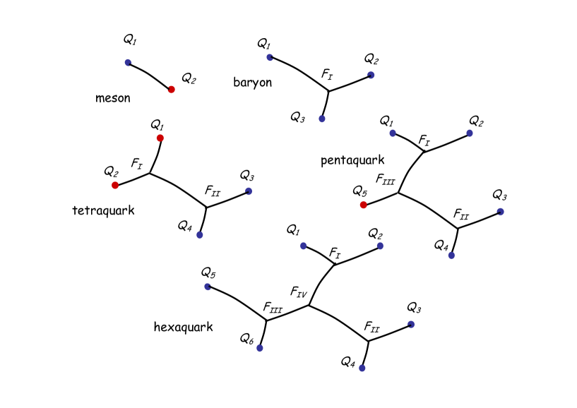
Figure 1: The geometries of the string sections linking the first five multiquarks. Notice that the number of Fermat points $F_{a}$ is $N-2$ where $N$ is the number of quarks and antiquarks $Q_{i}$ in the multiquark.

The geometries of the strings of the first five multiquarks are depicted in Fig. 1. Eq. (1) and Fig. 1 extend the definition of the Fermat point of a triangle to the Fermat point of polygons in three dimensions with more points. With the present definition, where confinement is produced by fundamental strings, the strings meet in internal three-string vertices. The number of quarks can always be increased replacing a quark (antiquark) by a Fermat point and a diquark (di-antiquark). Thus the number of quarks (and antiquarks) minus the number of Fermat points is a constant. Since in the meson and baryon this constant is 2, the number of Fermat points is $N-2$ where $N$ is the number of quarks and antiquarks. Moreover in eq. (1) we are only suming over distances between points linked by strings.

For a meson (quark-antiquark system) the distance is trivially the quark-antiquark distance. For a baryon (three quark system) the problem was first solved geometrically by Fermat and by Torricelli. In the case of 3 quarks, the minimization of the potential in eq. (1) implies that,

$$\widehat{r}_{1\,I}+\widehat{r}_{2\,I}+\widehat{r}_{3\,I}=0\ ,$$ (2)

and it is clear that the solution is that, either the triangle is not sufficiently acute, or the angles are all equal to $120^{o}$,

$$\widehat{\mathbf{r}_{1\,I},\mathbf{r}_{2\,I}}=\widehat{\mathbf{r}_{2\,I},\mathbf{r}_{3\,I}}=\widehat{\mathbf{r}_{3\,I},\mathbf{r}_{1\,I}}=120^{o}\ .$$ (3)

Due to the beauty of the triangles, and also to their simplicity, there are numerous geometry textbooks and articles on the Fermat - Torricelli point [1, 2, 3, 4, 5, 6, 7, 8, 9]. However, when the number of quarks increase, to tetraquarks, pentaquarks, etc, the geometric construction of the Fermat points becomes more and more difficult. Thus a numerical solution of this problem is welcome.

Here we address the computation of the total string distance and of the Fermat points where the different strings meet. In Section 2 we review briefly the geometrical methods leading to the Fermat points and to the total distances. In Section 3 we provide an iterative method, converging fast to the correct Fermat points and the total distances, relevant for the multiquark potentials. We detail the cases of the baryon, the tetraquark, the pentaquark and the hexaquark. In Section 4 we conclude.

2 Brief review of the geometrical method

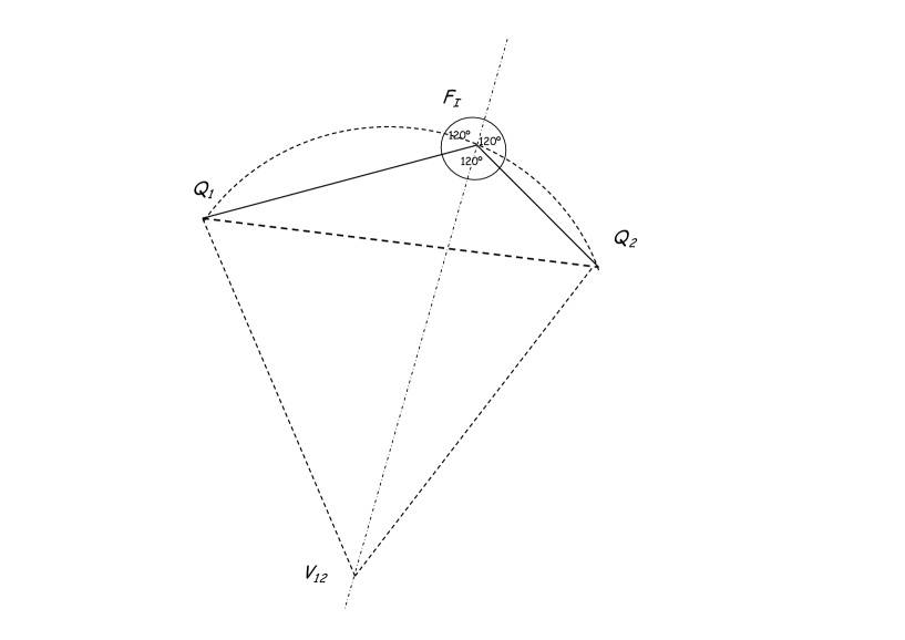
Figure 2: A step in the geometric construction of the first Fermat point of an acute triangle. Starting from the segment $Q_{1}\,Q_{2}$, an equilateral triangle with vertex $V_{12}$ is constructed. The Fermat point $F_{I}$ belongs to the arc of circle centered in $V_{12}$ and passing by $Q_{1}$ and $Q_{2}$.

In an acute triangle, the Fermat point $F_{I}$ is the isogonic point, defined in eq. (3). To construct the isogonic point, we start by the first pair of vertices $Q_{1}$ and $Q_{2}$, noticing that the set of points $F_{I}$ with fixed angle $\widehat{Q_{1}\,F_{I}\,Q_{2}}=120^{o}$ belong to an arc of circle. Moreover this circle is centred in the other vertex $V_{12}$ of an equilateral triangle including $Q_{1}$ and $Q_{2}$ . In Fig. 2 we show the $120^{o}$ arc of circle, the equilateral triangle, and a segment including the points $V_{12}$ and $F_{I}$. Notice that the other end of this segment forms with the segments $Q_{1}\,F_{I}$ and $F_{I}\,Q_{2}$ angles of $120^{o}$. Thus the isogonic point belongs this arc of circle. This point is at the intersection of the segments $V_{12}Q_{3}$, $V_{23}Q_{1}$ and $V_{31}Q_{2}$. The construction of first Fermat point $F_{I}$ is illustrated in Fig. 3. It is very simple in a geometrical perspective, and it can be done just with a compass and a rule.

Figure 3: The geometrical method to construct the Fermat $F_{I}$ point of a Baryon. The Fermat point is at the intersection fo the three segments $V_{12}Q_{3}$, $V_{23}Q_{1}$ and $V_{31}Q_{2}$.

We now proceed with the tetraquark. This geometrical method can be extended to construct the two Fermat points $F_{I}$ and $F_{II}$ of a tetraquark. Notice that in the tetraquark we have four points, and thus in general the points $Q_{1}$, $Q_{2}$, $Q_{3}$ and $Q_{4}$ are not coplanar. Thus the vertices $V_{12}$ and $V_{34}$ are not, from the onset determined, only the circles where they belong are determined with the technique already used for the baryon. To determine the vertices, notice that the vertex $V_{12}$ must be as far as possible from the segment $Q_{3}\,Q_{4}$ and that the vertex $V_{34}$ must be as far as possible from the segment $Q_{1}\,Q_{2}$. Thus we find that the segment $V_{12}\,V_{34}$ must intersect the segment $Q_{1}\,Q_{2}$ and the segment $Q_{3}\,Q_{4}$. Then, once the segment $V_{12}\,V_{34}$ is determined, the Fermat points $F_{I}$ and $F_{II}$ are determined because the distances $V_{12}\,F_{I}=Q_{1}\,Q_{2}$ and $V_{34}\,F_{II}=Q_{3}\,Q_{4}$. This is illustrated in Fig. 4.

Figure 4: The geometrical method to construct the two Fermat points $F_{I}$ and $F_{II}$ of a tetraquark. Notice that The points $Q_{1}$, $Q_{2}$, $Q_{3}$ and $Q_{4}$ are not coplanar. Thus the vertices $V_{12}$ and $V_{34}$ are not, from the onset determined, we only the circles where they belong. Nevertheless it is possible to determine tehm geometrically, knowing that the segment $V_{12}\,V_{34}$ intersects the segment $Q_{1}\,Q_{2}$ and the segment $Q_{3}\,Q_{4}$. Then, once the segment $V_{12}\,V_{34}$ is determined, the Fermat points $F_{I}$ and $F_{II}$ are determined because the distances $V_{12}\,F_{I}=Q_{1}\,Q_{2}$ and $V_{34}\,F_{II}=Q_{3}\,Q_{4}$.

Although the solutions are simple geometrically, the algebraic computation of the cartesian coordinates of the Fermat points $F_{a}$ is not simple. Let us consider the baryon case of triangle in a three dimensional space. We first need to check whether the triangle is acute. If the triangle is acute, we find each of the vertices $V_{ij}$ of the equilateral triangles with a system of three equations, two linear equations stating that the vertex belongs to the plane of $Q_{1}$, $Q_{2}$ and $Q_{3}$ and to the plane of the mediatrices of $Q_{i}$ and $Q_{j}$ , and one quadratic equation to fix the distance of the vertex to the medium point of $Q_{i}$ and $Q_{j}$. We have to ensure that the vertices $V_{ij}$ point outwards the initial triangle $Q_{1}\,Q_{2}\,Q_{3}$. To find the Fermat point $F_{I}$ we need to get two vertices, say $V_{12}$ and $V_{23}$, and then to intersect the segments $V_{12}Q_{3}$ and $V_{23}Q_{1}$. So we first need if statements, and in the acute case we have to solve a total of two quadratic equations and seven linear ones.

While this system of equations and inequations is exactly solvable for a triangle, the algebraic method gets quite difficult for larger multiquarks. Thus another method would be welcome to compute the Fermat points $F_{a}$ and the total distance $d=\sum_{i,a}r_{i\,a}$.

3 Iterative method

We now propose an iterative method, designed for a computational determination of the confining potential of multiquarks.

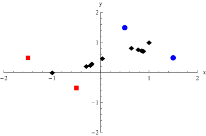
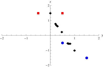
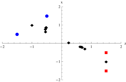
Figure 5: Convergence of the numerical iterative method method to construct the two Fermat points $F_{I}$ and $F_{II}$ of an arbitrary tetraquark. The quarks are depicted as circles, the antiquarks as squares, and the converging Fermat Points as diamonds. We show projections in the $xy$, $yz$ and $zx$ planes. Visually, after 6 iterations the iteration has converged. On average, a $10^{-6}$ precision is achieved for the tetraquark after 20 iterations.

We start from the triquark case of the baryon. We use the notation,

$$\mathbf{r}_{i} = (x_{i},y_{i},z_{i})\ ,$$

$$\mathbf{r}_{I} = (x_{I},y_{I},z_{I})\ ,$$

$$r_{i\,I} = \sqrt{(x_{I}-x_{i})^{2}+(y_{I}-y_{i})^{2}+(z_{I}-z_{i})^{2}}\ .$$ (4)

Minimizing the total distance $r_{1\,I}+r_{2\,I}+r_{3\,I}$ with regards to the three coordinates of the Fermat point $F_{I}$, we get the system equations,

$$x_{I} = {{x_{1}\over r_{1\,I}}+{x_{2}\over r_{2\,I}}+{x_{3}\over r_{3\,I}}\over{1\over r_{1\,I}}+{1\over r_{2\,I}}+{1\over r_{3\,I}}}\ ,$$

$$y_{I} = {{y_{1}\over r_{1\,I}}+{y_{2}\over r_{2\,I}}+{y_{3}\over r_{3\,I}}\over{1\over r_{1\,I}}+{1\over r_{2\,I}}+{1\over r_{3\,I}}}\ ,$$

$$z_{I} = {{z_{1}\over r_{1\,I}}+{z_{2}\over r_{2\,I}}+{z_{3}\over r_{3\,I}}\over{1\over r_{1\,I}}+{1\over r_{2\,I}}+{1\over r_{3\,I}}}\ .$$ (5)

which is non-linear. To solve these algebraic equations, of the form

$$x=X(x,y,z)\ ,$$

$$y=Y(x,y,z)\ ,$$

$$z=Z(x,y,z)\ ,$$ (6)

an iterative method can be used. With a relaxation coefficient $\omega$, we iterate the series,

$$x_{n+1} = \omega X(x_{n},y_{n},z_{n})+(1-\omega)x_{n}\ ,$$

$$y_{n+1} = \omega Y(x_{n},y_{n},z_{n})+(1-\omega)y_{n}\ ,$$

$$z_{n+1} = \omega Z(x_{n},y_{n},z_{n})+(1-\omega)z_{n}\ ,$$ (7)

starting with, as an initial guess, the barycentre

$${\mathbf{r}_{I}}_{0}={\mathbf{r}_{1}+\mathbf{r}_{2}+\mathbf{r}_{3}\over 3}\ .$$ (8)

A first numerical check shows that the method converges rapidly to the Fermat path of the triangle. We get get results accurate to a precision of $10^{-6}$, for the total distance $d=r_{1\,I}+r_{2\,I}+r_{3\,I}$ after a number of iterations of the order of 12, for an optimized relaxation factor $\omega=1.7$.

Thus we extend our iterarive method to the cases of the next multiquarks. We simply get a system of there equations per Fermat point. For the tetraquark the equations are,

$$x_{I} = {{x_{1}\over r_{1\,I}}+{x_{2}\over r_{2\,I}}+{x_{II}\over r_{{II}\,I}}\over{1\over r_{1\,I}}+{1\over r_{2\,I}}+{1\over r_{{II}\,I}}}\ ,$$

$$y_{I} = {{y_{1}\over r_{1\,I}}+{y_{2}\over r_{2\,I}}+{y_{II}\over r_{{II}\,I}}\over{1\over r_{1\,I}}+{1\over r_{2\,I}}+{1\over r_{{II}\,I}}}\ ,$$

$$z_{I} = {{z_{1}\over r_{1\,I}}+{z_{2}\over r_{2\,I}}+{z_{II}\over r_{{II}\,I}}\over{1\over r_{1\,I}}+{1\over r_{2\,I}}+{1\over r_{{II}\,I}}}\ ,$$

$$x_{II} = {{x_{3}\over r_{3\,{II}}}+{x_{4}\over r_{4\,{II}}}+{x_{I}\over r_{I\,{II}}}\over{1\over r_{3\,{II}}}+{1\over r_{4\,{II}}}+{1\over r_{I\,{II}}}}\ ,$$

$$y_{II} = {{y_{3}\over r_{3\,{II}}}+{y_{4}\over r_{4\,{II}}}+{y_{I}\over r_{I\,{II}}}\over{1\over r_{3\,{II}}}+{1\over r_{4\,{II}}}+{1\over r_{I\,{II}}}}\ ,$$

$$z_{II} = {{z_{3}\over r_{3\,{II}}}+{z_{4}\over r_{4\,{II}}}+{z_{I}\over r_{I\,{II}}}\over{1\over r_{3\,{II}}}+{1\over r_{4\,{II}}}+{1\over r_{I\,{II}}}}\ ,$$ (9)

and we also check that the iterations converge fast to the Fermat paths for the tetraquark. We illustrate graphically, for an arbitrary geometric configuration, the convergence in the case of a tetraquark in Fig. 5. For the pentaquark the equations are,

$$x_{I} = {{x_{1}\over r_{1\,I}}+{x_{2}\over r_{2\,I}}+{x_{III}\over r_{{III}\,I}}\over{1\over r_{1\,I}}+{1\over r_{2\,I}}+{1\over r_{{III}\,I}}}\ ,$$

$$y_{I} = {{y_{1}\over r_{1\,I}}+{y_{2}\over r_{2\,I}}+{y_{III}\over r_{{III}\,I}}\over{1\over r_{1\,I}}+{1\over r_{2\,I}}+{1\over r_{{III}\,I}}}\ ,$$

$$z_{I} = {{z_{1}\over r_{1\,I}}+{z_{2}\over r_{2\,I}}+{z_{III}\over r_{{III}\,I}}\over{1\over r_{1\,I}}+{1\over r_{2\,I}}+{1\over r_{{III}\,I}}}\ ,$$

$$x_{II} = {{x_{3}\over r_{3\,{II}}}+{x_{5}\over r_{5\,{II}}}+{x_{III}\over r_{{III}\,{II}}}\over{1\over r_{3\,{II}}}+{1\over r_{4\,{II}}}+{1\over r_{{III}\,{II}}}}\ ,$$

$$y_{II} = {{y_{3}\over r_{3\,{II}}}+{y_{4}\over r_{4\,{II}}}+{y_{III}\over r_{{III}\,{II}}}\over{1\over r_{3\,{II}}}+{1\over r_{4\,{II}}}+{1\over r_{{III}\,{II}}}}\ ,$$

$$z_{II} = {{z_{3}\over r_{3\,{II}}}+{z_{4}\over r_{4\,{II}}}+{z_{III}\over r_{{III}\,{II}}}\over{1\over r_{3\,{II}}}+{1\over r_{4\,{II}}}+{1\over r_{{III}\,{II}}}}\ ,$$

$$x_{III} = {{x_{I}\over r_{I\,{III}}}+{x_{II}\over r_{{II}\,{III}}}+{x_{4}\over r_{4\,{III}}}\over{1\over r_{I\,{III}}}+{1\over r_{{II}\,{III}}}+{1\over r_{5\,{III}}}}\ ,$$

$$y_{III} = {{y_{I}\over r_{I\,{III}}}+{y_{II}\over r_{{II}\,{III}}}+{y_{5}\over r_{5\,{III}}}\over{1\over r_{I\,{III}}}+{1\over r_{{II}\,{III}}}+{1\over r_{5\,{III}}}}\ ,$$

$$z_{III} = {{z_{I}\over r_{I\,{III}}}+{z_{II}\over r_{{II}\,{III}}}+{z_{5}\over r_{5\,{III}}}\over{1\over r_{I\,{III}}}+{1\over r_{{II}\,{III}}}+{1\over r_{5\,{III}}}}\ ,$$ (10)

multiquark	number	optimal	average number of iterations for a $p=$
	of quarks	$\omega$	$10^{-1}$	$10^{-2}$	$10^{-3}$	$10^{-4}$	$10^{-5}$	$10^{-6}$
meson	2	-	1	1	1	1	1	1
baryon	3	1.7	1.1	1.9	3	5	8	12
tetraquark	4	1.4	1.7	2.7	5	9	14	20
pentaquark	5	1.5	1.5	2.5	5	10	18	29
hexaquark	6	1.4	1.5	2.8	5	10	16	26

Table 1: Convergence of the iterative method for different multiquarks, based on a million of random generated quark positions, for each multiquark, and for different precisions $p={\Delta d\over d}$, where $d$ is the total Fermat distance. The values of the relaxation factor $\omega$ are the ones which minimize the convergence time up to a precision $p=10^{-6}$.

for the hexaquark the equations are,

$$x_{I} = {{x_{1}\over r_{1\,I}}+{x_{2}\over r_{2\,I}}+{x_{IV}\over r_{{IV}\,I}}\over{1\over r_{1\,I}}+{1\over r_{2\,I}}+{1\over r_{{IV}\,I}}}\ ,$$

$$y_{I} = {{y_{1}\over r_{1\,I}}+{y_{2}\over r_{2\,I}}+{y_{IV}\over r_{{IV}\,I}}\over{1\over r_{1\,I}}+{1\over r_{2\,I}}+{1\over r_{{IV}\,I}}}\ ,$$

$$z_{I} = {{z_{1}\over r_{1\,I}}+{z_{2}\over r_{2\,I}}+{z_{IV}\over r_{{IV}\,I}}\over{1\over r_{1\,I}}+{1\over r_{2\,I}}+{1\over r_{{IV}\,I}}}\ ,$$

$$x_{II} = {{x_{3}\over r_{3\,{II}}}+{x_{4}\over r_{4\,{II}}}+{x_{IV}\over r_{{IV}\,{II}}}\over{1\over r_{3\,{II}}}+{1\over r_{4\,{II}}}+{1\over r_{{IV}\,{II}}}}\ ,$$

$$y_{II} = {{y_{3}\over r_{3\,{II}}}+{y_{4}\over r_{4\,{II}}}+{y_{IV}\over r_{{IV}\,{II}}}\over{1\over r_{3\,{II}}}+{1\over r_{4\,{II}}}+{1\over r_{{IV}\,{II}}}}\ ,$$

$$z_{II} = {{z_{3}\over r_{3\,{II}}}+{z_{4}\over r_{4\,{II}}}+{z_{IV}\over r_{{IV}\,{II}}}\over{1\over r_{3\,{II}}}+{1\over r_{4\,{II}}}+{1\over r_{{IV}\,{II}}}}\ ,$$

$$x_{III} = {{x_{5}\over r_{5\,{III}}}+{x_{6}\over r_{6\,{III}}}+{x_{IV}\over r_{{IV}\,{III}}}\over{1\over r_{5\,{III}}}+{1\over r_{6\,{III}}}+{1\over r_{{IV}\,{III}}}}\ ,$$

$$y_{III} = {{y_{5}\over r_{5\,{III}}}+{y_{6}\over r_{6\,{III}}}+{y_{IV}\over r_{{IV}\,{III}}}\over{1\over r_{5\,{III}}}+{1\over r_{6\,{III}}}+{1\over r_{{IV}\,{III}}}}\ ,$$

$$z_{III} = {{z_{5}\over r_{5\,{III}}}+{z_{6}\over r_{6\,{III}}}+{z_{IV}\over r_{{IV}\,{III}}}\over{1\over r_{5\,{III}}}+{1\over r_{6\,{III}}}+{1\over r_{{IV}\,{III}}}}\ ,$$

$$x_{IV} = {{x_{I}\over r_{I\,{IV}}}+{x_{II}\over r_{{II}\,{IV}}}+{x_{III}\over r_{{III}\,{IV}}}\over{1\over r_{I\,{IV}}}+{1\over r_{{II}\,{IV}}}+{1\over r_{{III}\,{IV}}}}\ ,$$

$$y_{IV} = {{y_{I}\over r_{I\,{IV}}}+{y_{II}\over r_{{II}\,{IV}}}+{y_{III}\over r_{{III}\,{IV}}}\over{1\over r_{I\,{IV}}}+{1\over r_{{II}\,{IV}}}+{1\over r_{{III}\,{IV}}}}\ ,$$

$$z_{IV} = {{z_{I}\over r_{I\,{IV}}}+{z_{II}\over r_{{II}\,{IV}}}+{z_{III}\over r_{{III}\,{IV}}}\over{1\over r_{I\,{IV}}}+{1\over r_{{II}\,{IV}}}+{1\over r_{{III}\,{IV}}}}\ ,$$ (11)

and for larger multiquarks the extension of these equations is obvious.

The convergence of the method for the first multiquark systems is shown in Table 1 and in the Fig. 6

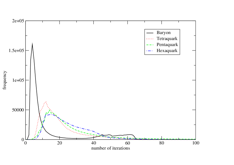
Figure 6: Distribution of the number of iterations needed to converge to a precision $p=10^{-6}$, based on a million of random generated quark positions, for each multiquark.

We study numerically the convergence of the method, with a randomly generated sample of $10^{6}$ geometric configurations, for each of the multiquarks. We first optimize the relaxation factor $\omega$ in order to reduce the needed number of iteration steps, to get results accurate to a precision of $10^{-6}$, for the total distance $d=\sum_{i,a}r_{i\,a}$. Since the number of iterations is not a constant, we demand the $\omega$ minimizing the average $\bar{d}$ over the sample of geometric configurations. The optimized $\omega$ and the resulting $\bar{d}$ are shown in Table 1 for the baryon, the tetraquark, the pentaquark and the hexaquark. Notice that the convergence is fast, even for the hexaquark.

Then we compute the distribution of the number of convergences we have per number of iterations. The number of configurations is large, and so we don’t need to join different numbers of iterations in a bin. In Fig. 6 we show the distribution of the number of distribution of the number of convergences we have per number of iterations for the baryon, the tetraquark, the pentaquark and the hexaquark.

4 Conclusion

We study an iterative method to find the Fermat points and Fermat distances in multiquarks. This method replaces the geometrical method, which has only been applied so far to the baryon (triquark).

The method is very simple to programme, and it converges both in the case of acute angles(smaller than $120^{o}$) and of larger angles. This avoids the problem of checking for non-acute angle, simple for a Baryon, but harder for the larger multiquarks.

This method is suited to be used in the solution of the Schrödinger equation in a quark model, where we have to compute the potential for several different positions of the quarks and antiquarks.

Thus we use, as a convergence criterion, the precision of $10^{-6}$, one part per million, in the total distance of the Fermat paths defined in Fig. 1. Even for this extremely fine precision, far beyond the normal precision of quark models, the method is quite fast, as show in Table 1. The number of necessary iterations $n$ to achieve a precision $p={\Delta d\over d}$, grows quadratically with the number of desired correct decimal cases, $-\log p$ is proportional to $n^{2}$.

The present computational technique enables the precision studies of the multiquarks with string confinement in the quark model.

References

• [1] Weisstein, Eric W. "Fermat Points." From MathWorld–A Wolfram Web Resource. http://mathworld.wolfram.com/FermatPoints.html
• [2] Gallatly, W. "The Isogonic Points." Β§151 in The Modern Geometry of the Triangle, 2nd ed. London: Hodgson, p. 107, 1913.
• [3] Greenberg, I. and Robertello, R. A. "The Three Factory Problem." Math. Mag. 38, 67-72, 1965.
• [4] van de Lindt, W. J. "A Geometrical Solution of the Three Factory Problem." Math. Mag. 39, 162-165, 1966.
• [5] Johnson, R. A. Modern Geometry: An Elementary Treatise on the Geometry of the Triangle and the Circle. Boston, MA: Houghton Mifflin, pp. 221-222, 1929.
• [6] Kimberling, C. "Central Points and Central Lines in the Plane of a Triangle." Math. Mag. 67, 163-187, 1994.
• [7] Kimberling, C. "Triangle Centers and Central Triangles." Congr. Numer. 129, 1-295, 1998.
• [8] Mowaffaq, H. "An Advanced Calculus Approach to Finding the Fermat Point." Math. Mag. 67, 29-34, 1994.
• [9] Spain, P. G. "The Fermat Point of a Triangle." Math. Mag. 69, 131-133, 1996.
• [10] J.Β Carlson, J.Β B.Β Kogut and V.Β R.Β Pandharipande, β€œA Quark Model For Baryons Based On Quantum Chromodynamics,” Phys.Β Rev.Β  D 27, 233 (1983).
• [11] T.Β T.Β Takahashi, H.Β Matsufuru, Y.Β Nemoto and H.Β Suganuma, β€œThe three-quark potential in the SU(3) lattice QCD,” Phys.Β Rev.Β Lett.Β  86, 18 (2001) [arXiv:hep-lat/0006005].
• [12] F.Β Okiharu, H.Β Suganuma and T.Β T.Β Takahashi, β€œThe tetraquark potential and flip-flop in SU(3) Lattice QCD,” Phys.Β Rev.Β  D 72, 014505 (2005) [arXiv:hep-lat/0412012].
• [13] F.Β Okiharu, H.Β Suganuma and T.Β T.Β Takahashi, β€œFirst study for the pentaquark potential in SU(3) Lattice QCD,” Phys.Β Rev.Β Lett.Β  94, 192001 (2005) [arXiv:hep-lat/0407001].
• [14] P.Β Bicudo, M.Β Cardoso and O.Β Oliveira, β€œFirst study of the gluon-quark-antiquark static potential in SU(3) Lattice QCD,” Phys.Β Rev.Β  D 77, 091504 (2008) [arXiv:0704.2156 [hep-lat]].
• [15] M.Β Cardoso and P.Β Bicudo, β€œFirst study of the three-gluon static potential in Lattice QCD,” Phys.Β Rev.Β  D 78, 074508 (2008) [arXiv:0807.1621 [hep-lat]].