Distilling entanglement from Fermions

Abstract

Since Fermions are based on anti-commutation relations, their entanglement can not be studied in the usual way, such that the available theory has to be modified appropriately. Recent publications consider in particular the structure of separable and of maximally entangled states. In this talk we want to discuss local operations and entanglement distillation from bipartite, Fermionic systems. To this end we apply an algebraic point of view where algebras of local observables, rather than tensor product Hilbert spaces play the central role. We apply our scheme in particular to Fermionic Gaussian states where the whole discussion can be reduced to properties of the covariance matrix. Finally the results are demonstrated with free Fermions on an infinite, one-dimensional lattice.

1. Introduction

Entanglement distillation is one of the most fundamental processes of quantum information processing [1]. It is an integral part of many protocols and devices like quantum repeaters and it provides important procedures to measure the entanglement content of a given physical system. In the usual setup it is assumed that two distant parties – Alice and Bob – share a large number of (weakly) entangled pairs of particles, and the task is to generate a (possibly small) amount of highly (or even maximally) entangled pairs by means of local operations and classical communication. In this context it is implicitly assumed that the particles shared by Alice and Bob are distinguishable: Firstly there is a clear distinction between particles controlled by Alice and those controlled by Bob. Secondly many distillation protocols require the selection of particular pairs by Alice and Bob (e.g. to perform filtering operations). Hence even the local particles needs to be distinguishable.

At a first glance it therefore appears to be completely impossible to talk about entanglement distillation with fermions, because the latter are by definition undistinguishable. A second thought reveals, however, very quickly that this is only an apparent difficulty. The only thing we have to drop is the focus on particles. Instead we have to consider setups where Alice and Bob control independent subsystems (usually distinguished by their position in space) of a larger physical system. A typical example is a Fermi gas from which Alice and Bob want to distill entanglement by using only operations (together with classical communication) which are localized in spatially separated regions (e.g. Alice’s and Bob’s laboratories).

Mathematically such a situation is most easily described in terms of operator algebras. In other words, instead of using tensor products of Hilbert spaces, we describe bipartite systems by specifying which local observables are measurable by Alice and which by Bob. This approach is successfully applied to the study of entanglement of infinite degrees of freedom systems [11, 7] and for the analysis of separable [8, 5] and maximally entangled [9] states of Fermionic systems (cf. also the references in [5] for more literature on Fermionic entanglement).

The purpose of this paper is to study entanglement distillation in the same framework. In this context we will show that distillation from Fermions can be treated basically in the same way as ordinary distillation with only some small changes which mainly arise from the emergence of super selection rules. In addition we will present an explicit scheme which can be applied to any quasi-free state and which allows explicit calculations (e.g. of distillation rates) for fairly large systems, such as (subsystems of) infinite quasi-free lattice models.

2. Entanglement distillation

Let us start with a short look on standard distillation techniques. Hence assume that Alice and Bob share $N$ $d$-level systems in the joint state $\rho^{\otimes N}$, where $\rho$ denotes a density matrix on the Hilbert space $\mathcal{H}\otimes\mathcal{H}$, $\mathcal{H}=\mathbb{C}^{d}$. To generate maximally entangled qubit pairs from these resources they can proceed as follows:

1. Look for (and drop) unentangled subsystems. Mathematically this means to find a unitary $U:\mathcal{H}\rightarrow\mathcal{H}_{1}\otimes\mathcal{K}$, $\mathcal{H}_{1}=\mathbb{C}^{d_{1}}$, and to apply the transformation $T_{1}(\rho)=\operatorname{tr}_{\mathcal{K}}(U\rho U^{*})$. The final state $\rho_{1}$ should contain (almost) as much entanglement as the original $\rho$. In other words: $\mathcal{K}$ and $U$ has to be chosen appropriately.

2. Find a maximally entangled state $\psi\in\mathcal{H}_{1}\otimes\mathcal{H}_{1}$ such that

   $$\langle\psi,\rho_{1}\psi\rangle>d_{1}^{-1}.$$ (1)

   The best choice would be to take the $\psi$ which maximizes this fidelity. To be successful here the first step is in many cases mandatory, because a state can be entangled without satisfying inequality (1) for any maximally entangled $\psi$. This can be easily seen if we choose $d=2\tilde{d}$ and

   $$\rho=|\phi\rangle\langle\phi|\otimes\frac{{\leavevmode{\rm 1\mkern-4.8muI}}}{\tilde{d}^{2}}\quad\phi=2^{-1/2}(|00\rangle+|11\rangle)$$ (2)

   since we get $\sup_{\psi}\langle\psi,\rho\psi\rangle=1/\tilde{d}^{2}$, which can be arbitrarily small (if $\tilde{d}$ is big enough) although $\rho$ is distillable.

3. Consider the group

   $$G_{\psi}=\{U_{A}\otimes U_{B}\,|\,U_{A},U_{B}\in\operatorname{U}(d_{1}),\ U_{A}\otimes U_{B}\psi=\psi\},$$ (3)

   and average over it. This leads to the twirl operation given by

   $$T_{2}(\rho_{1})=\int_{G_{\psi}}U\rho U^{*}dU,$$ (4)

   where $dU$ denotes the Haar measure on $G_{\psi}$.

4. The output of the channel $T_{2}$ is an isotropic state

   $$\rho_{2}=T_{2}\rho_{1}=\vartheta|\psi\rangle\langle\psi|+(1-\vartheta)\frac{{\leavevmode{\rm 1\mkern-4.8muI}}}{d_{1}^{2}}$$ (5)

   with $\vartheta\in[-(d_{1}^{2}-1)^{-1},1]$ given in terms of the fidelity $f=\langle\psi,\rho\psi\rangle$ by

   $$\vartheta=\frac{d_{1}^{2}f-1}{d_{1}^{2}-1}.$$ (6)

   From Equation (1) it follows immediately that $\rho_{2}$ again satisfies the inequality

   $$\langle\psi,\rho_{2}\psi\rangle>d_{1}^{-1},$$ (7)

   and therefore it is distillable [6].

5. Now we can continue with standard techniques for isotropic states which provide us with a number $M$ of (almost) maximally entangled qubit pairs; cf [12] and the references therein.

3. Bipartite Fermionic systems

To study entanglement of Fermionic systems the usual framework which relies on tensor product Hilbert spaces is too narrow because indistinguishability and anti-commutation relations has to be taken into account. Instead, it is more appropriate to describe the splitting of the overall system into two subsystems in terms of observables algebras. This approach was successfully applied in particular to infinite degrees of freedom systems [11, 7]. For our purposes a simplified (finite dimensional) approach is sufficient.

• A bipartite quantum system consists of a Hilbert space and two C*-algebras $\mathcal{A},\mathcal{B}\subset\mathcal{B}(\mathcal{H})$ which commute elementwise (i.e. $[A,B]=0$ $\forall A\in\mathcal{A}$, $\forall B\in\mathcal{B}$).

Selfadjoint elements of $\mathcal{A}$ and $\mathcal{B}$ describe the (projection valued) observables of the given system which can be locally measured by Alice and Bob respectively. The default setup can be recovered if we have

$$\mathcal{A}=\mathcal{B}(\mathcal{H}_{A})\otimes{\leavevmode{\rm 1\mkern-4.8muI}}_{B},\quad\mathcal{B}={\leavevmode{\rm 1\mkern-4.8muI}}_{A}\otimes\mathcal{B}(\mathcal{H}_{B}),\quad\mathcal{M}=\mathcal{B}(\mathcal{H}_{A}\otimes\mathcal{H}_{B})$$ (8)

in terms of two Hilbert spaces $\mathcal{H}_{A},\mathcal{H}_{B}$. Note, however, that we have neither assumed that $\mathcal{A}$ and $\mathcal{B}$ together generate $\mathcal{B}(\mathcal{H})$ nor that $\mathcal{B}$ is the commutant of $\mathcal{A}$ (in contrast to [7]). Therefore beside (8) other realizations of bipartite systems are possible, even if $\mathcal{H}$ is finite dimensional. A particular example arises, if $\mathcal{H}_{A/B}$ decomposes into a direct sum $\mathcal{H}_{A/B}=\mathcal{H}_{A/B}^{+}\oplus\mathcal{H}_{A/B}^{-}$, and if we define

$$\mathcal{A}=\bigl{(}\mathcal{B}(\mathcal{H}_{A}^{+})\oplus\mathcal{B}(\mathcal{H}_{A}^{-})\bigr{)}\otimes{\leavevmode{\rm 1\mkern-4.8muI}}_{B},\quad\mathcal{B}={\leavevmode{\rm 1\mkern-4.8muI}}_{B}\otimes\bigl{(}\mathcal{B}(\mathcal{H}_{A}^{+})\oplus\mathcal{B}(\mathcal{H}_{A}^{-})\bigr{)}.$$ (9)

This is – as we will see – exactly the situation we have to study for a system consisting of a finite number of Fermions.

To explain the latter remark consider the Hilbert space $\mathcal{K}$ and the corresponding antisymmetric Fockspace $\mathcal{H}=\mathcal{F}_{-}(\mathcal{K})$. For each $h,f\in\mathcal{K}$ we can define the usual creation and annihilation operators $c^{*}(h)$ and $c(f)$ on $\mathcal{H}$, which satisfy the canonical anti-commutation relations ($\{\,\cdot\,,\,\cdot\,\}$ denotes the anti-commutator)

$$\{c(f),c(h)\}=\{c^{*}(f),c^{*}(h)\}=0,\quad\{c^{*}(h),c(f)\}=\langle h,f\rangle{\leavevmode{\rm 1\mkern-4.8muI}}.$$ (10)

In some cases it is more convenient to combine $c$ and $c^{*}$ in one operator (this is called the self-dual formalism [2, 3]):

$$B(f,h)=c(f)+c^{*}(\overline{h}),\quad\Gamma(f,h)=(\overline{h},\overline{f}),$$ (11)

where $(\overline{\,\cdot\,})$ denotes complex conjugation in an appropriately chosen (and fixed!) basis. Now we get from (10)

$$\{B(F_{1}),B(F_{2})\}=\langle\Gamma F_{1},F_{2}\rangle,\quad B(F)^{*}=B(\Gamma F),\forall F,F_{1},F_{2}\in\mathcal{K}\oplus\mathcal{K}.$$ (12)

The set of operators $\{c(f)\,|\,f\in\mathcal{K}\}\subset\mathcal{B}(\mathcal{H})$ generates a C*-algebra $\operatorname{CAR}(\mathcal{K})\subset\mathcal{B}(\mathcal{H})$ which is called the algebra of canonical ani-commutation relations. It can be regarded as the closure (in operator norm) of the algebra of polynomials in the $c(f)$ and $c^{*}(h)$.

Now consider the parity operator on $\mathcal{H}$ which is given in terms of the number operator $N$ by $\theta=(-1)^{N}$. It acts as the identity on the subspace $\mathcal{H}^{+}\subset\mathcal{H}$ of vectors with an even particle number and as minus the identity on the complementary subspace $\mathcal{H}^{-}$. We write $P^{\pm}$ for the corresponding projections and get

$$P^{\pm}:\mathcal{H}\rightarrow\mathcal{H}^{\pm},\quad\theta=P^{+}-P^{-}.$$ (13)

The elements of $\operatorname{CAR}(\mathcal{K})$ which commute with $\theta$ are called even elements and they form the even subalgebra

$$\operatorname{CAR}_{+}(\mathcal{K})=\{A\in\operatorname{CAR}(\mathcal{K})\,|\,[A,\theta]=0\}$$ (14)

of $\operatorname{CAR}(\mathcal{K})$. It can be regarded as the (closure of) the algebra of even polynomials in $c(f)$ and $c^{*}(h)$.

If $\mathcal{K}$ is finite dimensional $\operatorname{CAR}(\mathcal{K})$ coincides with $\mathcal{B}(\mathcal{H})$, i.e. it is a full matrix algebra. The even subalgebra however is given by

$$\operatorname{CAR}_{+}(\mathcal{K})=\mathcal{B}(\mathcal{H}^{+})\oplus\mathcal{B}(\mathcal{H}^{-}).$$ (15)

This can be easily seen from the fact that a product of an even number of creation and annihilation operators can change the particle number only by a factor of 2.

The next step is to decompose $\mathcal{K}$ into an “Alice” and a “Bob” subspace, i.e. $\mathcal{K}=\mathcal{K}_{A}\oplus\mathcal{K}_{B}$. Then we can associate to $\mathcal{K}_{A/B}$ the corresponding Fockspaces $\mathcal{H}_{A/B}=\mathcal{F}_{-}(\mathcal{K}_{A/B})$, and also the CAR-algebras $\operatorname{CAR}(\mathcal{K}_{A/B})$ and $\operatorname{CAR}_{+}(\mathcal{K}_{A/B})$. Obviously we have

$$\mathcal{H}=\mathcal{F}_{-}(\mathcal{K})\cong\mathcal{F}_{-}(\mathcal{K}_{A})\otimes\mathcal{F}_{-}(\mathcal{K}_{B})=\mathcal{H}_{A}\otimes\mathcal{H}_{B},$$ (16)

and similarly $\operatorname{CAR}(\mathcal{K})$ is isomorphic to $\operatorname{CAR}(\mathcal{K}_{A})\otimes\operatorname{CAR}(\mathcal{K}_{B})$ if we consider the spatial tensor product. The corresponding isomorphism satisfies

$$c(f_{A}\oplus 0)\mapsto c_{A}(f_{A})\otimes{\leavevmode{\rm 1\mkern-4.8muI}}_{B},\quad c(0\oplus f_{B})\mapsto\theta_{B}\otimes c_{B}(F_{B}),$$ (17)

where the $c_{A/B}(f_{A/B})$ denote the annihilation operators and $\theta_{A/B}$ the parity operators on $\mathcal{H}_{A/B}$. The latter are related to the global parity $\theta$ by

$$\theta=\theta_{A}\otimes\theta_{B}.$$ (18)

Equation (17) shows that $\operatorname{CAR}(\mathcal{K}_{A/B})$ can not both be embedded as tensor factors into $\operatorname{CAR}(\mathcal{K})$ without violating the anti-commutation relations. The construction given in (17) is therefore called the twisted tensor product of $\operatorname{CAR}(\mathcal{K}_{A})$ and $\operatorname{CAR}(\mathcal{K}_{B})$.

The discussion of the last paragraph has shown that two operators $A\in\operatorname{CAR}(\mathcal{K}_{A})$, $B\in\operatorname{CAR}(\mathcal{K}_{B})$ do not commute in general and therefore these two algebras can not be chosen as the observable algebras $\mathcal{A}$ and $\mathcal{B}$. If we choose, however, $A$ and $B$ to be even elements we immediately get from (17) that $[A,B]=0$ holds. Hence

$$\mathcal{A}=\operatorname{CAR}_{+}(\mathcal{K}_{A}),\quad\mathcal{B}=\operatorname{CAR}_{+}(\mathcal{K}_{B})$$ (19)

is an appropriate choice for the local observable algebras of Alice and Bob. Together they define a bipartite Fermionic system in the sense of Definition 3. If $\mathcal{K}_{A}$ and $\mathcal{K}_{B}$ are finite dimensional we can insert Equation (15) for $\mathcal{A}$ and $\mathcal{B}$ and we recover the example already given in (8). Note in addition that $\mathcal{A}\subset\mathcal{B}(\mathcal{H}_{A})$ and $\mathcal{B}\subset\mathcal{B}(\mathcal{H}_{B})$ holds, while the full CAR algebras fail to have this property – by virtue of Equation (17). Hence it is reasonable to consider $\mathcal{H}_{A}$ ($\mathcal{H}_{B}$) as Alice’s (Bob’s) Hilbert space.

4. Local operations

On top of the scheme described in the last section all basic notions of entanglement theory can be reconstructed. This was done for separable states in [8, 5] and for maximally entangled states in [9]. To discuss entanglement distillation we need the concept of a local operation which can be defined as follows (cf. [7]):

• Consider two bipartite systems $\mathcal{A}_{j},\mathcal{B}_{j}\subset\mathcal{B}(\mathcal{H}_{j})$, $j=1,2$. An operation (i.e. a completely positive map) $T:\mathcal{B}(\mathcal{H}_{1})\rightarrow\mathcal{B}(\mathcal{H}_{2})$ is called local if

  $$T(\mathcal{A}_{1})\subset\mathcal{A}_{2},\quad T(\mathcal{B}_{1})\subset\mathcal{B}_{2}$$ (20)

  and

  $$T(AB)=T(A)T(B)\quad\forall A\in\mathcal{A}_{1},\ \forall B\in\mathcal{B}_{1}$$ (21)

  holds.

In the standard framework (8) with finite dimensional Hilbert spaces $\mathcal{H}_{A},\mathcal{H}_{B}$ (or if we assume that the operation $T$ is normal) this definition coincides with the usual one. Note that the factorization condition (21) is needed to make this statement true [7].

To generalize the distillation protocol from Section 2. only a few special local operations are needed. They are summarized in the following list.

• Local unitaries. The easiest case is a local unitary transformation $A\mapsto U^{*}AU$ with $U=U_{A}\otimes U_{B}$ and $U_{A}$ ($U_{B}$) unitary on $\mathcal{H}_{A}$ ($\mathcal{H}_{B}$). It is easy to see that $U_{A}^{*}\mathcal{A}U_{A}=\mathcal{A}$ is equivalent to $U_{A}\mathcal{H}_{A}^{\pm}=\mathcal{H}_{A}^{\pm}$ or $U_{A}\mathcal{H}_{A}^{\pm}=\mathcal{H}_{A}^{\mp}$. A similar statement holds for $U_{B}$.

• Local Bogolubov transformations. A special case of the previous example arises if $U_{A}$ and $U_{B}$ are related to unitaries $u_{A}$, $u_{B}$ on $\mathcal{K}_{A}\oplus\mathcal{K}_{A}$, $\mathcal{K}_{B}\oplus\mathcal{K}_{B}$ by

  $$U^{*}B(F)U=B(uF),\ \text{with}\ U=U_{A}\otimes U_{B},\ u=u_{A}\oplus u_{B},$$ (22)

  where $B(F)$ is the operator introduced in Equation (11). It is easy to see that (22) is only possible if

  $$\Gamma u\Gamma=u$$ (23)

  holds (cf. again (11)). The condition (23) is on the other hand sufficient for the existence of a unitary $U$ satisfying (22) for a given $u$.

• Discarding subsystems. Consider now decompositions $\mathcal{K}_{A/B}=\mathcal{K}_{A/B,1}\oplus\mathcal{K}_{A/B,2}$ of $\mathcal{K}_{A}$ and $\mathcal{K}_{B}$. If we denote the Fockspaces of $\mathcal{K}_{j}=\mathcal{K}_{A,j}\oplus\mathcal{K}_{B,j}$, $j=1,2$ by $\mathcal{H}_{j}$ we get a decomposition of $\mathcal{H}$ into a tensor product $\mathcal{H}=\mathcal{H}_{1}\otimes\mathcal{H}_{2}$. If we perform the partial trace over say $\mathcal{H}_{2}$ we get the Fockspace $\mathcal{H}_{1}$ and the corresponding reduced observable algebras $\mathcal{A}_{1},\mathcal{B}_{1}\subset\mathcal{B}(\mathcal{H}_{1})$. In this way the partial trace becomes (the Schrödinger picture version of) a local operation between two bipartite Fermionic systems, which discards the modes belonging to $\mathcal{K}_{2}$.

• A joint parity measurement is described by the PVM

  $$P^{jk}=P_{A}^{j}\otimes P_{B}^{k},\quad j,k=+,-$$ (24)

  and the corresponding von Neumann-Lüders instrument ($P_{A/B}^{\pm}$ denote the projections to the even/odd subspaces of $\mathcal{H}_{A}$ and $\mathcal{H}_{B}$; cf. Section 3.). For a system in the state $\rho$ the probability to get the outcome $j,k$ is $p^{jk}$ and the corresponding output state is $\rho^{jk}$:

  $$p^{jk}=\operatorname{tr}(P^{jk}\rho),\quad\rho^{jk}=\frac{P^{jk}\rho P^{jk}}{p^{jk}}.$$ (25)

  The projections $P^{jk}$ commute with all $A\in\mathcal{A}$ and all $B\in\mathcal{B}$. Therefore parity measurements can be done without disturbing the system. This implies immediately that the state $\rho$ can not be distinguished from the mixture $\sum_{jk}p^{jk}\rho^{jk}$. Within a distillation scheme this instrument can be used to perform local filtering operations; e.g. Alice and Bob can decide to drop the whole system if their local parities are different and to keep it otherwise. If we set

  $$\mathcal{K}_{A}=\mathcal{K}_{B}=\mathbb{C}^{d}\Rightarrow\mathcal{H}_{A}^{+}\cong\mathcal{H}_{A}^{-}\cong\mathcal{H}_{B}^{+}\cong\mathcal{H}_{B}^{-}\cong\mathbb{C}^{D},\quad D=2^{d-1},$$ (26)

  and ignore the value of the parities (apart from $j=k$) we get a (non-unital) local operation which transforms a bipartite Fermionic system into a pair of $D-$level systems in the state

  $$\frac{p^{++}\rho^{++}+p^{--}\rho^{--}}{p^{++}+p^{--}}.$$ (27)

5. Distilling from Fermions

Let us now adopt the general distillation scheme sketched in Section 2. to the Fermionic case. To this end we will use throughout this section the assumptions made in Equation (26), which implies in particular that (9) holds. In addition, consider two maximally entangled vectors $\varphi_{+}\in\mathcal{H}^{++}$, $\varphi_{-}\in\mathcal{H}^{--}$ and

$$\psi_{\pm}=\frac{1}{\sqrt{2}}(\varphi_{+}\pm\varphi_{-}).$$ (28)

For each $A\in\mathcal{A}\otimes\mathcal{B}$ we have

$$\operatorname{tr}(A|\psi_{\pm}\rangle\langle\psi_{\pm}|)=\frac{1}{2}\left(\operatorname{tr}(A|\varphi_{+}\rangle\langle\varphi_{+}|)+\operatorname{tr}(A|\varphi_{-}\rangle\langle\varphi_{-}|)\right).$$ (29)

Using the terminology from Equations (45) and (57) this can be rewritten as:

$$p^{++}=p^{--}=\frac{1}{2},\ p^{+-}=p^{-+}=0,\ \rho^{++}=|\varphi_{+}\rangle\langle\varphi_{+}|,\ \rho^{--}=|\varphi_{-}\rangle\langle\varphi_{-}|.$$ (30)

Hence Alice and Bob can not distinguish the vector states $|\psi_{\pm}\rangle\langle\psi_{\pm}|$ from themselves and from the mixture of $|\varphi_{+}\rangle\langle\varphi_{+}|$ with $|\varphi_{-}\rangle\langle\varphi_{-}|$. The latter is according to [9] a Fermionic maximally entangled state (implying in particular that EOF is maximal).

The only step from the list in Section 2. we have to change is the twirling, because averaging over the group $G_{\psi_{+}}$ (or $G_{\psi_{-}}$) breaks the superselection rule and is therefore not an allowed local operation. Instead, we have to look at the subgroup

$$H_{\psi_{+}}=\{U_{A}\otimes U_{B}\in G_{\psi_{+}}\,|\,U_{A}\mathcal{A}U_{A}=\mathcal{A},\quad U_{B}\mathcal{B}U_{B}=\mathcal{B}\}.$$ (31)

The structure of this group is given by the following Proposition

• The group $H_{\psi_{+}}$ is generated by the subgroup

  $$H_{\psi_{+},0}=\{U_{A}\otimes U_{B}\in G_{\psi_{+}}\,|\,[U_{A},\theta_{A}]=0,\quad[U_{B},\theta_{B}]=0\}$$ (32)

  and $V=V_{A}\otimes V_{B}$ given by

  $$V_{A}e_{A,j}^{+}=e_{A,j}^{-},\quad V_{B}e_{B,j}^{+}=e_{B,j}^{-}$$ (33)

  where $e_{A/B,j}^{\pm}$, $j=1,\dots,D$, $D=2^{d-1}$ are given in terms of the Schmidt decomposition of $\varphi_{\pm}$, i.e.

  $$\varphi_{+}=\frac{1}{\sqrt{D}}\sum_{j=1}^{D}e_{A,j}^{+}\otimes e_{B,j}^{+},\quad\varphi_{-}=\frac{1}{\sqrt{D}}\sum_{j=1}^{D}e_{A,j}^{-}\otimes e_{B,j}^{-}.$$ (34)

Proof.  Obviously $H_{\psi_{+},0}\subset H_{\psi_{+}}$ and $V_{A}\otimes V_{B}\in H_{\psi_{+}}$. To show the other inclusion recall from the discussion of local unitaries in the last section that $U_{A}\mathcal{A}U_{B}^{*}=\mathcal{A}$ is equivalent to $U_{A}\mathcal{H}_{A}^{\pm}=\mathcal{H}_{A}^{\pm}$ (i.e. $[U_{A},\theta_{A}]=0$) or $U_{A}\mathcal{H}_{A}^{\pm}=\mathcal{H}_{A}^{\mp}$, and that a similar statement holds for $U_{B}$. The assumption $U_{A}\otimes U_{B}\psi_{+}=\psi_{+}$ implies in addition that $[U_{A},\theta_{A}]=0\Leftrightarrow[U_{B},\theta_{B}]=0$ holds. Hence $U\in H_{\psi_{+}}$ is either in $H_{\psi_{+},0}$ or it can be written as $U=\tilde{U}V$ with a $\tilde{U}\in H_{\psi_{+},0}$, which concludes the proof. $\Box$

Averaging over the group $H_{\psi_{+}}$ leads to states which are $H_{\psi_{+}}$ invariant. Their structure is given by the following proposition.

• Each $H_{\psi_{+}}$-invariant state $\sigma$ can be written as

  $$\sigma=\lambda_{+}|\psi_{+}\rangle\langle\psi_{+}|+\lambda_{-}|\psi_{-}\rangle\langle\psi_{-}|+\mu_{+}(P^{++}+P^{--})+\mu_{-}(P^{+-}+P^{-+})$$ (35)

  with

  $$p^{++}=p^{--}=\frac{\lambda_{+}+\lambda_{-}}{2}+\mu_{+}D^{2},\quad p^{-+}=p^{+-}=\mu_{-}D^{2},$$ (36)

  $$\langle\psi_{\pm},\sigma\psi_{\pm}\rangle=\lambda_{\pm}+\mu_{+}.$$ (37)

Proof.  We have to determine the commutant $H_{\psi_{+}}^{\prime}$ of $H_{\psi_{+}}$. To this end note first that $H_{\psi_{+},0}\subset H_{\psi_{+}}$ implies $H_{\psi_{+}}^{\prime}\subset H_{\psi_{+},0}^{\prime}$. Hence consider the latter commutant first. By definition we have for each unitary $U$ on $\mathcal{H}_{A}\otimes\mathcal{H}_{B}$

$$U\in H_{\psi_{+},0}\Leftrightarrow[U,|\psi_{+}\rangle\langle\psi_{+}|]=0,\ [U,\theta_{A}\otimes{\leavevmode{\rm 1\mkern-4.8muI}}]=0,\ [U,{\leavevmode{\rm 1\mkern-4.8muI}}\otimes\theta_{B}]=0,$$ (38)

where we have used the fact that the factorization $U=U_{A}\otimes U_{B}$ is a consequence of $[U,\psi_{+}]=0$; cf. [13]. Therefore $H_{\psi_{+},0}^{\prime}$ is the von Neumann algebra generated by $|\psi_{+}\rangle\langle\psi_{+}|$, $\theta_{A}\otimes{\leavevmode{\rm 1\mkern-4.8muI}}$ and ${\leavevmode{\rm 1\mkern-4.8muI}}\otimes\theta_{B}$, i.e.

$$H_{\psi_{+},0}^{\prime}=\{|\psi_{+}\rangle\langle\psi_{+}|,\theta_{A}\otimes{\leavevmode{\rm 1\mkern-4.8muI}},{\leavevmode{\rm 1\mkern-4.8muI}}\otimes\theta_{B}\}^{\prime\prime}.$$ (39)

By calculating all possible products of the generators this leads to

$$H_{\psi_{+},0}^{\prime}=\operatorname{span}\{|\psi_{+}\rangle\langle\psi_{+}|,|\psi_{-}\rangle\langle\psi_{-}|,|\psi_{+}\rangle\langle\psi_{-}|,|\psi_{-}\rangle\langle\psi_{+}|,\\ P^{++},P^{--},P^{+-},P^{-+}\}.$$ (40)

The group $H_{\psi_{+}}$ is generated by $H_{\psi_{+},0}$ and $V=V_{A}\otimes V_{B}$; cf. Proposition 5. Hence $A\in\mathcal{H}_{\psi_{+},0}^{\prime}$ is in $\mathcal{H}_{\psi_{+}}^{\prime}$ iff it commutes $V$. Since $V_{A}$ and $V_{B}$ just exchanges the even with the odd subspace we easily conclude that

$$H_{\psi_{+}}^{\prime}=\operatorname{span}\{|\psi_{+}\rangle\langle\psi_{+}|,|\psi_{-}\rangle\langle\psi_{-}|,P^{++}+P^{--},P^{+-}+P^{-+}\}$$ (41)

holds, which implies equation (35). Equations (36) and (37) follow immediately from the definition of the $p^{jk}$ in (45) and from taking traces. $\Box$

If we decompose the $H_{\psi_{+}}$-invariant state $\sigma$ according to Equation (57) we get

$$\sigma^{\pm\pm}=\frac{\lambda_{+}+\lambda_{-}}{2p^{\pm\pm}}|\varphi_{\pm}\rangle\langle\varphi_{\pm}|+\frac{\mu_{+}}{p^{\pm\pm}}P^{\pm\pm}\quad\sigma^{\pm\mp}=\frac{P^{\pm\mp}}{D^{2}}.$$ (42)

Hence if Alice and Bob perform $\theta_{A},\theta_{B}$ measurements – which they can do without disturbing the systems – they get either with probability

$$p=p^{++}+p^{--}$$ (43)

one of the (basically equivalent) isotropic states $\sigma^{++}$ or $\sigma^{--}$, or they get with probability $1-p$ the totally chaotic state $\sigma^{+-}$ or $\sigma^{-+}$. In case they get $\sigma^{\pm\pm}$ it is distillable iff

$$\langle\varphi_{\pm},\sigma^{\pm\pm}\varphi_{\pm}\rangle>\frac{1}{D}$$ (44)

holds. A straightforward calculation using Equations (36), (37), (42) and (44) leads to the following proposition

• Consider a state $H_{\psi_{+}}$ invariant state $\sigma$. The fidelity $f=\langle\varphi_{\pm},\sigma^{\pm\pm}\varphi_{\pm}\rangle$ of the isotropic state $\sigma^{\pm\pm}$ from Equation (42) is given by

  $$f=\frac{\langle\psi_{+},\sigma\psi_{+}\rangle+\langle\psi_{-},\sigma\psi_{-}\rangle}{p}.$$ (45)

  Hence $\sigma^{\pm\pm}$ is distillable iff

  $$\langle\psi_{+},\sigma\psi_{+}\rangle+\langle\psi_{-},\sigma\psi_{-}\rangle>\frac{p}{D}$$ (46)

  holds.

Let us start with a general state $\rho$ and twirl over $H_{\psi_{+}}$, i.e.

$$\sigma=\int_{H_{\psi_{+}}}U\rho U^{*}dU.$$ (47)

Then $\sigma$ is $H_{\psi_{+}}$ invariant and Equation (46) is equivalent to

$$\langle\psi_{+},\rho\psi_{+}\rangle+\langle\psi_{-},\rho\psi_{-}\rangle>\frac{p}{D}$$ (48)

To get a general distillation protocol for Fermionic systems we can therefore modify the distillation presented in Section 2. as follows:

1. Start with $N$ distinguishable copies of the same Fermionic system, each prepared in the same state (e.g. $N$ metallic wires containing an electron gas).

2. Drop unentangled subsystems. This leads to $N$ bipartite Fermionic systems in the joint state $\rho^{\otimes N}$. Here $\rho$ is a density operator on $\mathcal{H}_{A}\otimes\mathcal{H}_{B}$, which should be interpreted, however, as a state of the algebra $\mathcal{A}\otimes\mathcal{B}$.

3. Find maximally entangled states $\psi_{\pm}$ as in Equation (28) such that (48) holds.

4. Average over the group $H_{\psi_{+}}$. This leads to the $H_{\psi_{+}}$-invariant state $\sigma$.

5. Make $\theta_{A},\theta_{B}$ measurement. If the outcome is $++$ or $--$ (which happens with probability $p$) this leads to the isotropic state $\sigma^{++}$ or $\sigma^{--}$. It can be treated with standard distillation techniques.

6. Otherwise ($+-$, $-+$) we get a chaotic state which is useless for distillation.

To find a maximally entangled state $\psi_{+}$ such that (48) is satisfied usually requires an optimization over all possible $\psi_{+}$. In general this is very difficult. In the next section, however, we will discuss a special class of states where this problem is more feasible and which provide at the same time a systematic way of dropping unentangled modes.

6. Quasifree states

Let us apply the general scheme developed in the last section to quasifree states. Recall that a density matrix $\rho$ describes a quasifree state of the CAR algebra $\operatorname{CAR}(\mathcal{K})$ if there is a bounded operator $S\in\mathcal{B}(\mathcal{K})$ such that

$$\operatorname{tr}(\rho B(f_{1})\cdots B(f_{2n+1}))=0$$ (49)

$$\operatorname{tr}(\rho B(f_{1})\cdots B(f_{2n}))=\sum\operatorname{sign}(p)\prod_{j=1}^{n}\langle\Gamma f_{p(2j-1)},Sf_{p(2j)}\rangle,$$ (50)

holds for all $n\in\mathbb{N}$ and $f_{k}\in\mathcal{K}\oplus\mathcal{K}$. The sum in (50) is taken over all permutations $p$ satisfying

$$p(1)<p(3)<...<p(2n-1),\quad p(2j-1)<p(2j)$$ (51)

and $\operatorname{sign}(p)$ is the signature of $p$. The covariance operator $S$ is selfadjoint and satisfies

$$\Gamma S\Gamma=1-S,\quad 0\leq S\leq{\leavevmode{\rm 1\mkern-4.8muI}}.$$ (52)

We can express the right hand side of Equation (50) as the Pfaffian $\operatorname{Pf}(\tilde{S})$ of the antisymmetric matrix $\tilde{S}$ with matrix elements $\tilde{S}_{jk}=\langle f_{j},Sf_{k}\rangle$ $k>j$. Note also that this definition works as well in infinite dimensions, although we will restrict our discussion in this chapter again to the case $\mathcal{K}_{A}=\mathcal{K}_{B}=\mathbb{C}^{d}$, $\mathcal{K}=\mathcal{K}_{A}\oplus\mathcal{K}_{B}$. In $\mathcal{K}_{A/B}\oplus\mathcal{K}_{A/B}$ we will use the bases ($k=1,\dots,2d$)

$$e_{A/B}^{(k)}=\begin{cases}e_{A/B,1}^{(k)}=2^{-1/2}(|k\rangle+|k+d\rangle)&\text{if $k\leq d$}\\ e_{A/B,2}^{(k-d)}=2^{-1/2}i(|k-d\rangle-|k\rangle)&\text{if $k>d$}\end{cases}$$ (53)

where $|k\rangle$, $k=1,\dots 2d$ denotes the canonical basis in $\mathbb{C}^{2d}$. If the decomposition into Alice- and Bob-subsystems is not important we can also use relabeled version

$$e^{(k)}=\begin{cases}e_{A}^{(k)}&\text{for $k\leq 2d$}\\ e_{B}^{(2d-k)}&\text{for $k>2d$}\end{cases}$$ (54)

where $k$ ranges now from $1$ to $4d$. The advantage of this basis is its $\Gamma$ invariance. We can therefore write

$$S_{kj}=\langle e^{(k)},Se^{(j)}\rangle=\langle\Gamma e^{(k)},Se^{(j)}\rangle,$$ (55)

with $k,j=1,\dots,4d$. In the following we will identify with slight abuse of notation the operator $S$ with the matrix $(S_{jk})_{j,k}$ and write

$$S=\left(\begin{array}[]{cc}S_{AA}&S_{AB}\\ S_{BA}&S_{BB}\end{array}\right)=\frac{1}{2}\left(\begin{array}[]{cc}{\leavevmode{\rm 1\mkern-4.8muI}}_{A}+iX&iY\\ -iY^{T}&{\leavevmode{\rm 1\mkern-4.8muI}}_{B}+iZ\end{array}\right).$$ (56)

These expressions should be interpreted as block matrices with respect to the Alice/Bob split, e.g. $S_{AB}$ contains all matrix elements of the form $\langle e_{A}^{(j)},Se_{B}^{(k)}\rangle$, etc. Using Equation (52) it is easy to see that $X,Y,Z$ are real $2d\times 2d$ matrices, and that $Y,Z$ are antisymmetric.

For quasifree states the expressions and constructions from the last two sections can be given quite explicitly in terms of covariance matrices. The following list summarizes the most important examples (cf. [10] for more details, in particular for proofs)

• The probability $p$ to get equal parities during a joint $\theta_{A},\theta_{B}$ measurement (cf. Equation (43) is given by

  $$p=\frac{1+(-4)^{d}\operatorname{Pf}(S-{\leavevmode{\rm 1\mkern-4.8muI}}/2)}{2}.$$ (57)

• A quasifree state with covariance matrix $P$ is maximally entangled, iff $P$ has (in the basis from Equation (53)) the form

  $$P=\frac{1}{2}\left(\begin{array}[]{cc}{\leavevmode{\rm 1\mkern-4.8muI}}_{A}&iR\\ -iR^{T}&{\leavevmode{\rm 1\mkern-4.8muI}}_{B}\end{array}\right),$$ (58)

  with a real orthogonal matrix $R$. The quasifree state thus given can be represented by a state vector $\psi_{P}\in\mathcal{H}$ with

  $$\psi_{P}=\frac{1}{\sqrt{2}}(\varphi_{+}+\varphi_{-})$$ (59)

  with maximally entangled vectors $\varphi_{\pm}\in\mathcal{H}_{A}^{\pm}\otimes\mathcal{H}_{B}^{\pm}$. In other words $\psi_{P}$ is always of the form $\psi_{+}$ assumed in Equation (28).

• The fidelity between a quasifree state $\rho_{S}$ and a maximally entangled quasifree state $\psi_{P}$ is given by

  $$\langle\psi_{P},\rho\psi_{P}\rangle=\operatorname{Pf}({\leavevmode{\rm 1\mkern-4.8muI}}-S-P).$$ (60)

• The quasifree state $\rho_{S}$ can be transformed by a local Bogolubov transformation $u$ into a normal form $\rho_{\tilde{S}}$ (which is again quasifree) such that the off diagonal blocks $-i\tilde{S}_{AB}$ and $i\tilde{S}_{BA}$ of the covariance matrix $\tilde{S}=uSu^{*}$ become diagonal with positive eigenvalues. To see this consider the singular value decomposition $Y=u_{A}\Sigma_{Y}u_{B}^{*}$ of $Y$ and choose $u=u_{A}\oplus u_{B}$.

The general distillation scheme described in the last section comprises the search for a $\psi_{+}$ such that Equation (48) holds. Since we can always choose $\psi_{+}=\psi_{P}$ for some $P$ satisfying (58) a good strategy is optimize the expression in (60) over all such $P$. The following theorem treats an important special case (cf. [10] for a proof).

• Consider a quasifree state $\rho_{S}$ with covariance matrix $S$ from Equation (56). Assume that $X=0$ or $Z=0$ holds, and that $Y$ is diagonal with non-negative eigenvalues (the latter can be done without loss of generality). The maximal fidelity of $\rho_{S}$ with a quasifree, maximally entangled state $\psi_{P}$ arises if the basis projection $P$ is given by

  $$P=\frac{1}{2}\left(\begin{array}[]{cc}{\leavevmode{\rm 1\mkern-4.8muI}}_{A}&i{\leavevmode{\rm 1\mkern-4.8muI}}\\ -i{\leavevmode{\rm 1\mkern-4.8muI}}&{\leavevmode{\rm 1\mkern-4.8muI}}_{B}\end{array}\right),$$ (61)

  and its value is

  $$\langle\psi_{P},\rho\psi_{P}\rangle=\prod_{j=1}^{n}\left(\frac{1+\lambda_{j}}{2}\right)^{m_{j}}$$ (62)

  where $\lambda_{j}$, $j=1,\dots,n$ denote the eigenvalues values of $Z$ and $m_{j}$ the corresponding multiplicities.

If the condition $X=0$ or $Z=0$ is not satisfied the optimality statement is in general not true. For states, however, which are already close to a maximally entangled, quasi free state $X$ and $Z$ have to be at least small (otherwise the condition $0\leq S\leq{\leavevmode{\rm 1\mkern-4.8muI}}$ is not satisfied). Hence in this case the choice $\psi_{P}$ with $P$ from (61) should be close to the optimum (provided $Y$ is diagonalized). Therefore the following specialization of the procedure from the last section should provide a reasonably good scheme for distillation from quasi free, Fermionic states.

1. Consider $N$ bipartite Fermionic systems, each of which in the same quasi free state $\rho_{S}$.

2. Choose bases for $\mathcal{K}_{A}\oplus\mathcal{K}_{A}$ and $\mathcal{K}_{B}\oplus\mathcal{K}_{B}$ such that the block-offdiagonal part $Y$ of $S$ becomes diagonal (and with real positive entries). As already pointed out above this can be done locally by Alice and Bob without any communication (if $S$ is known to them).

3. Drop all modes except those belonging to the $n$ highest singular values of $Y$. The number $n$ must be chosen such that Equation (48) holds with $\psi_{+}=\psi_{P}$ where the basis projection $P$ is (in basis which diagonalizes $Y$) of the form (61). The maximally entangled state $\psi_{-}$ is then quasi free as well, i.e. $\psi_{-}=\psi_{Q}$ with basis projection

   $$Q=\frac{1}{2}\left(\begin{array}[]{cc}{\leavevmode{\rm 1\mkern-4.8muI}}_{A}&-i{\leavevmode{\rm 1\mkern-4.8muI}}\\ i{\leavevmode{\rm 1\mkern-4.8muI}}&{\leavevmode{\rm 1\mkern-4.8muI}}_{B}\end{array}\right)$$ (63)

   (please check yourself). Hence the two fidelities $\langle\psi_{\pm}\rho_{S},\psi_{\pm}\rangle$ in Equation (48) can be calculated with (61). If the probability $p$ is unknown Equation (48) should be used with the conservative choice $p=1$.

4. Average (twirl) over the group $H_{\psi_{+}}$, make a $\theta_{A},\theta_{B}$ measurement and proceed as described in Section 5.

Let us demonstrate this scheme with free fermions (without spin) hopping on a one-dimensional regular lattice $\mathbb{Z}$ (lets call it a “wire”). They can be described by the CAR algebra $\operatorname{CAR}(\mathrm{l}^{2}(\mathbb{Z}))$ and the dynamics is given formally by the Hamiltonian

$$H=\sum_{j\in\mathbb{Z}}\left(c_{j}^{*}c_{j+1}+c_{j+1}^{*}c_{j}\right).$$ (64)

It admits a unique quasifree ground state $\varphi_{0}$ with covariance operator $S$ given by

$$S=\mathcal{F}^{-1}\left(\begin{array}[]{cc}E&0\\ 0&1-E\end{array}\right)\mathcal{F}$$ (65)

where

$$\mathrm{l}^{2}(\mathbb{Z})\otimes\mathbb{C}^{2}\ni F\mapsto\mathcal{F}(F)\in\mathrm{L}^{2}(S^{1})\otimes\mathbb{C}^{2},\quad\mathcal{F}(F)(x)=\sum_{j=-\infty}^{\infty}e^{inx}F_{n}$$ (66)

is the Fourier transform and $E\in\mathcal{B}(\mathrm{L}^{2}(S^{1}))$ the projection to the upper half-circle [2, 4].

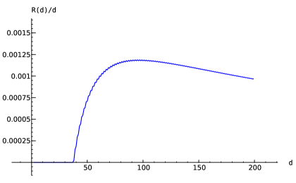
Fig. 1: Distillation rate $R(d)/d$ for free Fermions on a one-dimensional lattice, if only two adjacent regions of length $d$ are accessed.

Now assume that Alice and Bob can control only two blocks of the form $\Lambda_{A}=[0,d)$ and $\Lambda_{B}=[d,2d)$ (or any joint spatial translate of them). The restriction to the corresponding subsystem leads exactly to the bipartite Fermionic system just studied. The reduced density matrix $\rho_{\Lambda}$ arising from the ground state $\varphi_{0}$ is quasifree and its covariance matrix in the basis (54) can be easily derived from (65).

Now we can apply the distillation protocol given above. If we choose to keep in step 3 only the four highest singular values of $Y$ we get at the end with probability $p$ from (57) a qubit pair in an isotropic state $\sigma=f|\phi\rangle\langle\phi|+(1-f)({\leavevmode{\rm 1\mkern-4.8muI}}-|\phi\rangle\langle\phi|)/3$, with fidelity $f$ from Equation (45). If a large number of systems is available (where system refers here to a whole wire not to a single Fermion) and if the fidelity $f$ is big enough we can use the Hashing protocol to distill maximally entangled qubit pairs. The distillation rate, i.e. the number of maximally entangled pairs we get asymptotically per wire is [12]

$$R=p\bigl{(}1-S(\sigma)\bigr{)}=p\bigl{(}1+f\log_{2}(f)+(1-f)\log_{2}(1-f)-(1-f)\log_{2}(3)\bigr{)}.$$ (67)

Maybe more interesting is the rate $R/d$ of pairs we get per lattice site used. The result is plotted in Figure 1. The small zigzag noise on the graph arises from a slightly different behavior of the protocol for even and odd values for $d$. This is an indication that the scheme is indeed not optimal if the assumptions from Theorem 6. (i.e. $X=0$ or $Z=0$) are not satisfied.

References

• [1] G. Alber, T. Beth, M. Horodecki, R. Horodecki, M. Rötteler, H. Weinfurter, R. Werner and A. Zeilinger (editors). Quantum information. Springer, Berlin (2001).
• [2] H. Araki. On quasifree states of ${\rm CAR}$ and Bogoliubov automorphisms. Publ. Res. Inst. Math. Sci. 6, 385–442 (1970/71).
• [3] H. Araki. Bogoliubov automorphisms and Fock representations of canonical anticommutation relations. In Operator algebras and mathematical physics (Iowa City, Iowa, 1985), volume 62 of Contemp. Math., pages 23–41. Amer. Math. Soc., Providence, RI (1987).
• [4] H. Araki and T. Matsui. Ground states of the $XY$-model. Comm. Math. Phys. 101, no. 2, 213–245 (1985).
• [5] M.-C. Bañuls, J. I. Cirac and M. M. Wolf. Entanglement in fermionic systems. Phys. Rev. A 76, 022311 (2007).
• [6] M. Horodecki and P. Horodecki. Reduction criterion of separability and limits for a class of distillation protocols. Phys. Rev. A 59, no. 6, 4206–4216 (1999).
• [7] M. Keyl, T. Matsui, D. Schlingemann and R. F. Werner. Entanglement, Haag-duality and type properties of infinite quantum spin chains. Rev. Math. Phys. 18, no. 9, 935–970 (2006).
• [8] H. Moriya. On separable states for composite systems of distingushable fermions. J. Phys. A 39, 3753–3762 (2006).
• [9] D. Schlingemann, M. Cozzini, M. Keyl and L. Campos Venuti. Maximally entangled fermions. Phys. Rev. A 78, 032301 (2008).
• [10] L. Campos Venuti, Z. Kadar, M. Keyl and D. Schlingemann. Entanglement distillation with quasifree fermions. in preparation.
• [11] R. Verch and R. F. Werner. Distillability and positivity of partial transposes in general quantum field systems. Rev. Math. Phys. 17, no. 5, 545–576 (2005).
• [12] K. G. Vollbrecht and M. M. Wolf. Efficient distillation beyond qubits. Phys. Rev. A 67, 012303 (2003).
• [13] K. G. H. Vollbrecht and R. F. Werner. Entanglement measures under symmetry. Phys. Rev. A 64, 062307 (2001).