Strong Spatial Mixing and Approximating Partition Functions of Two-State Spin Systems without Hard Constrains

Abstract: We prove Gibbs distribution of two-state spin systems(also known as binary Markov random fields) without hard constrains on a tree exhibits strong spatial mixing(also known as strong correlation decay), under the assumption that, for arbitrary ‘external field’, the absolute value of ‘inverse temperature’ is small, or the ‘external field’ is uniformly large or small. The first condition on ‘inverse temperature’ is tight if the distribution is restricted to ferromagnetic or antiferromagnetic Ising models.

Thanks to Weitz’s self-avoiding tree, we extends the result for sparse on average graphs, which generalizes part of the recent work of Mossel and Sly[15], who proved the strong spatial mixing property for ferromagnetic Ising model. Our proof yields a different approach, carefully exploiting the monotonicity of local recursion. To our best knowledge, the second condition of ‘external field’ for strong spatial mixing in this paper is first considered and stated in term of ‘maximum average degree’ and ‘interaction energy’. As an application, we present an FPTAS for partition functions of two-state spin models without hard constrains under the above assumptions in a general family of graphs including interesting bounded degree graphs.

Keywords: Strong Spatial Mixing; Self-Avoiding Trees; Two-State Spin Systems; Ising Models; FPTAS; Partition Function

I Introduction

Counting problem has played an important role in theoretic computer science since Valiant[19] introduced $\#$P-Complete conception and proved many enumeration problems are computationally intractable. The most successful and powerful existing method for counting problem is due to Markov Chain method, which has been successfully used to provide a fully polynomial randomized approximation schemes (FPRAS)(which approximates the real value within a factor of $\epsilon$ in polynomial time of the input and $\epsilon^{-1}$ with the probability $\geq$ 3/4) for convex bodies[3] and the number of perfect matchings on bipartite graphs[9]. Since many counting problems such as the number of matchings, independent sets, circuits[14] etc. can be viewed as special cases of computing partition functions associated with Gibbs measures in statistical physics. Hence studying the computation of partition function is a natural extension of counting problems.

Self-reducing [10] or conditional probability method is a well known method to compute partition functions if the marginal probability of a vertex can be efficiently approximated. Gibbs sampling also known as Glauber dynamics is a popular used method to approximate marginal probability. This is a Markov Chain approach locally updating the chain according to conditional Gibbs measure. Hence studying the convergence rate(also known as mixing time) of Glauber dynamics becomes a major research direction. Recently the problem whether the Glauber dynamics converges ‘fast’(in a polynomial time of the input and logarithm of reciprocal of sampling error) deeply related to whether a phase transition takes place in statistical model has been extensively studied, see [16] for hard core model(also known as independent set model) and [15][6] for ferromagnetic Ising model. Another approach to approximate marginal probability comes from the property of the structure of Gibbs measures on various graphs. This method utilizes local recursion and leads to deterministic approximation schemes rather than random approximation schemes of Markov Chain method. Our paper focuses on this recursive approach.

The recursive approach for counting problems is introduced by Weitz[21] and Bandyopadhyay, Gamarnik [1] for counting the number of independent sets and colorings. The key of this method is to establish the $strong$ $spatial$ $mixing$ property also known as $strong$ $correlation$ $decay$ on certain defined rooted trees, which means the marginal probability of the root is asymptotically independent of the configuration on the leaves far below. Usually the exponential decay with the distance implies a deterministic polynomial time approximating algorithm for marginal probability of the root. In [21], Weitz establishes the equivalence between the marginal probability of a vertex in a general graph $G$ and that of the root of a tree named $self$-$avoiding$ $tree$ associated with $G$ for two-state spin systems and shows the correlations on any graph decay at least as fast as its corresponding self-avoiding tree. He also proves the strong correlation decay for hard-core model on bounded degree trees. Later Gamarnik et.al.[5] and Bayati et.al.[2] bypass the construction of a self-avoiding tree, by instead creating a certain $computation$ $tree$ and establishing the strong correlation decay on the corresponding computation tree for list coloring and matchings problems. An interesting relation between self-avoiding tree and computation tree is that they share the same recursive formula for hard-core model. Considering the motivation of construction of the self-avoiding tree, Jung and Shah[8] and Nair and Tetali [17] generalize Weitz’s work for certain Markov random field models, and Lu et.al.[12] for TP decoding problem. Mossel and Sly[15] show ferromagnetic Ising model exhibits strong correlation decay on ‘sparse on average’ graph under the tight assumption that the ‘inverse temperature’ in term of ‘maximum average degree’ is small.

In this paper, based on self-avoiding tree, we establish the strong spatial mixing for general two-state spin systems also know binary Markov random field without hard constrains on a graph that are sparse on average under certain assumptions. Our first condition is on the ‘inverse temperature’. We show that there exits a value $J_{d}$ in term of ‘maximum average degree’ $d$, if the absolute value of the ‘inverse temperature’ is smaller than $J_{d}$, for arbitrary ‘external field’, the Gibbs measure exhibits strong spatial mixing on a sparse on average graph. Since for (anti)ferromagnetic Ising model, strong spatial mixing on a finite regular tree implies uniqueness of Gibbs measures of infinite regular tree[4][20]. $J_{d}$ in our setting is the critical point for uniqueness of Gibbs measures of infinite regular tree with degree of each vertex $d$, implying our condition is also necessary on trees. The condition is the same as that of Mossel and Sly[15] when ferromagnetic Ising model is the only focus. This makes part of their work in our framework. Our proof yields a different approach, and also avoids the argument between weak spatial mixing and strong spatial mixing employed in [21]. In fact our proof is based an inequality similar to the one in [13] and carefully exploits monotonicity of the recursive formula. The recursive formula on trees is well known. Recently Pemantle and Peres [18] use it to present the exact capacity criteria that govern behavior at critical point of ferromagnetic Ising model on trees under various boundary conditions. Our second condition is for ‘external field’. We prove for any ‘inverse temperature’ on a graph which are sparse on average Gibbs distribution exhibits strong spatial mixing when the ‘external field’ is uniformly larger than $B(d,\alpha_{\max},\gamma)$ or smaller than $-B(d,-\alpha_{\min},\gamma)$, where $d$ is ‘maximum average degree’ and $\alpha_{\min}$, $\alpha_{\max}$, $\gamma$ are parameters of the system. To our best knowledge, this condition on ‘external field’ is first considered for strong spatial mixing. The technique employed in the proof is Lipchitz approach which has been used in [1][2][5]. The novelty here is that we propose a ‘path’ characterization of this method, allowing us to give the ‘external field’ condition in term of ‘maximum average degree’ rather than maximum degree. Some notations of the ‘sparse on average’ graphs have appeared in [15]. These are graphs where the sum degrees along each self-avoiding path(a path with distinct vertices) with length $O($log$n)$ is $O($log$n)$.

As an application of our results, we present a fully polynomial time approximation schemes(FPTAS)(which approximates the real value within a factor of $\epsilon$ in polynomial time of the input and $\epsilon^{-1}$) for partition functions of two-state spin systems without hard constrains under our assumptions on the graph $G=(V,E)$, where, for each vertex $v\in V$ of $G$, the number of total vertices of its associated self-avoiding tree $T_{saw(v)}$ with hight $O($log$n)$ is $O(n^{O(1)})$. This includes bounded degree graph and especially $Z^{d}$ lattice more concerned in statistical physics. Jerrum and Sinclair [7] provided an FPRAS for partition function of ferromangetic Ising model for any graph with any positive ‘inverse temperature’ and identical external field for all the vertices. Their results do not include the case where different vertices have different external field, and are not applied to antiferromagnetic Ising model where the ‘inverse temperature’ is negative either.

The remainder of the paper has the following structure. In Section II, we present some preliminary definitions and main results. We go on to prove the theorems in Section III. Section IV is devoted to propose an FPTAS for the partition functions under our conditions. Further work and conclusion are given in Section IV.

II Preliminaries and Main Results

II-A Two-State Spin Systems

In the two-state spin systems on a finite graph $G=(V,E)$ with vertices $V=\{1,2,\cdots,n\}$ and edge set $E$, a configuration consists of an assignment $\sigma=(\sigma_{i})$ of $\Omega=\{\pm 1\}$ values, or “spins”, to each vertex(or“sites”) of $V$. Each vertex $i\in V$ is associated with a random variable $X_{i}$ with range ${\pm 1}$. We often refer to the spin values $\pm 1$ as $(+)$ and $(-)$. The probability of finding the system in configuration $\sigma\in\Omega^{n}$ is given by the joint distribution of $n$ dimensional random vector $X=\{X_{1},X_{2},\cdots,X_{n}\}$(also known as the Gibbs distribution with the nearest neighbor interaction)

$$P_{G}(X=\sigma)=\frac{1}{Z(G)}\exp(\sum\limits_{(i,j)\in E}\beta_{ij}(\sigma_{i},\sigma_{j})+\sum\limits_{i\in V}h_{i}(\sigma_{i})).$$

Here $Z(G)$ is called partition function of the system and a normalized factor such that $\sum_{\sigma\in\Omega^{n}}P_{G}(X=\sigma)=1$, and $h_{i}$ and $\beta_{ij}$ are defined as a function from $\Omega$ and $\Omega^{2}$ to $R\cup\{\pm\infty\}$ respectively. We use notation $\beta_{ij}(a,b)=\beta_{ji}(b,a)$. We say the system has hard constraints if there exit an edge $(i,j)\in E$ or a vertex $k$, and an assignment $\sigma_{i}$, $\sigma_{j}$ or $\sigma_{k}$ such that $\beta_{ij}(\sigma_{i};\sigma_{j})=\infty$ or $h_{k}(\sigma_{k})=\infty$ (e.g. hard-core model is one of the systems with hard constrains where $\beta_{ij}(+,+)=-\infty$, $\beta_{ij}(+,-)=\beta_{ij}(-,+)=\beta_{ij}(-,-)=0$ and $h_{i}(-)=0$). In this paper we focus to the systems without hard constrains. We call the function $\beta_{ij}$ ‘interaction energy’ and $h_{i}$ ‘applied field’ . If $\beta_{ij}(\sigma_{i},\sigma_{j})=J_{ij}\sigma_{i}\sigma_{j}$ and $h_{i}=B_{i}\sigma_{i}$ for all the edge $(i,j)\in E$ and vertex $i\in V$, where $J_{ij}$ and $B_{i}$ are constant numbers varying with edges or vertices, the system is called Ising model. Further, if $J_{ij}$ is uniformly (negative)positive for all $(i,j)\in E$, the system is called (anti)ferromagnetic Ising model. $J_{ij}$ and $B_{i}$ are called $inverse$ $temperature$ and $external$ $field$ respectively. To match the notation of Ising model, set $J_{ij}=\frac{\beta_{ij}(+,+)+\beta_{ij}(-,-)-\beta_{ij}(-,+)-\beta_{ij}(+,-)}{4}$ and $B_{i}=\frac{h_{i}(+)-h_{i}(-)}{2}$ for all edges and vertices , in this paper we call $J_{ij}$ and $B_{i}$ are ‘inverse temperature’ and ‘external field’ of general two-state spin systems without hard constrains (denoted by TSSHC for abbreviation)respectively. For any $\Lambda\subseteq V$, $\sigma_{\Lambda}$ denotes the set $\{\sigma_{i},i\in\Lambda\}$. With a little abuse of notations, $\sigma_{\Lambda}$ also denotes the configuration that $i$ is fixed $\sigma_{i}$, $\forall i\in\Lambda$. Let $Z(G,\Phi)$ denote the partition function under the condition $\Phi$, e.g. $Z(G,X_{1}=+)$ represent the partition function under the condition the vertex $1$ is fixed $+$.

II-B Definitions and Notations

Definition 2.1 (Self-Avoiding Tree) Consider a graph $G=(V,E)$ and a vertex $v\in V$ in $G$. Given any order of all the vertices in $G$. There is associated partial order on $E$ of the order on $V$ defined as $(i,j)>(k,l)$ iff $(i,j)$, $(k,l)$ share a common vertex and $i+j>k+l$. The self-avoiding tree $T_{saw(v)}(G)$(for simplicity denoted by $T_{saw(v)}$) corresponding to the vertex $v$ is the tree of self-avoiding walks originating at $v$ except that the vertices closing a cycle are also included in the tree and are fixed to be either $+$ or $-$. Specifically, the vertex of the $T_{saw(v)}$ closing a cycle is fixed $+$ if the edge ending the cycle is larger than the edge starting the cycle and $-$ otherwise. Given any configuration $\sigma_{\Lambda}$ of $G$, $\Lambda\subset V$, the self-avoiding tree is constructed the same as the above procedure except that the vertex which is a copy of the vertex $i$ in $\Lambda$ is fixed to the same spin $\sigma_{i}$ as $i$ and the subtree below it is not constructed(See Figure 1). Hence, for any configuration $\sigma_{\Lambda}$ of $G$, $\Lambda\subset V$, we also use $\sigma_{\Lambda}$ to denote the configuration of $T_{saw(v)}$ obtained by imposing the condition corresponding to $\sigma_{\Lambda}$ as above. For any $(i,j)\in E$ and $i\in V$ of $G$, the ‘interaction energy’ function and ‘applied field’ function on all their copies of the induced system on $T_{saw(v)}$ by $G$ are the same as $\beta_{ij}$ and $h_{i}$ respectively.

We now provide the remarkable property of the self-avoiding tree, one of two main results of [21], which is one of the essential techniques of our proofs.

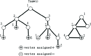
Figure 1: The graph with one vertex assigned + (Right)and its corresponding self-avoiding tree $T_{saw(1)}$(Left)

Proposition 2.1 For two-state spin systems on $G=(V,E)$, for any configuration $\sigma_{\Lambda}$, $\Lambda\subset V$ and any vertex $v\in V$, then

$$P_{G}(X_{v}=+|\sigma_{\Lambda})=P_{T_{saw(v)}}(X_{v}=+|\sigma_{\Lambda}).$$

In order to generalize our result to more general families of graphs , which are sparse on average, we need some definitions and notation of these graphs.

Definition 2.2 Let $|A|$ denote the cardinality of the set $A$. The length of a path is the number of edges it contains. The distance of two vertices in a graph is the length of shortest path connecting these two vertices. A path $v_{1},v_{2},\cdots$ is called a self-avoiding path if for all $i\neq j$ , $v_{i}\neq v_{j}$. In a graph $G=(V,E)$, let $d(u,v)$ denote the distance between $u$ and $v$, $u$,$v\in V$. The distance between a vertex $v\in V$ and a subset $\Lambda\subset V$ is defined by $d(v,\Lambda)=$min$\{d(v,u):u\in\Lambda\}$. The set of vertices within distance $l$ of $v$ is denoted by $V(G,v,l)=\{u:d(v,u)\leq l\}$. Similarly, the set of vertices with distance $l$ of $v$ is denoted by $S(G,v,l)=\{u:d(v,u)=l\}$. We call a vertex at the height $t$ of a rooted tree if the distance between it and the root is $t$. Let $\delta_{v}$ denote the degree of $v$ in $G$. The $maximal$ $path$ $density$ $m$ is defined by $m(G,v,l)=\max\limits_{\Gamma}\sum\limits_{u\in\Gamma}\delta_{u}$, where the maximum is taken over all self-avoiding paths $\Gamma$ starting at $v$ with length at most $l$. The $maximum$ $average$ $path$ $degree$ $\delta(G,v,l)$ is defined by $\delta(G,v,l)=(m(G,v,l)-\delta_{v})/l,l\geq 1$. The $maximum$ $average$ $degree$ of $G$ is defined by $\Delta(G,l)=\max_{v\in V}\delta(G,v,l)$. Roughly speaking, in this paper, a family of graphs $\mathcal{G}$ is sparse on average if there exits a constant number $a$ and $d$ such that $\Delta(G,a\log n)\leq d$ for any $G\in\mathcal{G}$.

Some properties of the above definitions are useful in our proof, we present them. Most of proofs are simply obtained by induction and can be found in [15].

Proposition 2.2 Let $j$, $l$ denote positive natural numbers, then

$$m(G,v,jl)\leq j\max\limits_{u\in G}\{m(G,u,l)-\delta_{u}\}+\delta_{v}.$$

Proposition 2.3 Let $l$ be natural numbers, then

$$|S(T_{saw(v)},v,l+1)|\leq\delta_{v}(\delta(G,v,l)-1)^{l}.$$

Proposition 2.4 Let $j$, $l$ be natural numbers, then

$$|V(T_{saw(v)},v,jl)|\leq(\max\limits_{u\in V}|V(T_{saw(u)},u,l)|)^{j}.$$

Definition 2.3 ((Exponential) Strong Spatial Mixing) Let $G=(V,E)$ be a graph with $n$ vertices. The Gibbs distribution of two-state spin systems on $G$ exhibits strong spatial mixing iff for any vertex $v\in V$, subset $\Lambda\subset V$, any two configurations $\sigma_{\Lambda}$ and $\eta_{\Lambda}$ on $\Lambda$, denote $\Theta=\{v\in\Lambda:\sigma_{v}\neq\eta_{v}\}$ and $t=d(v,\Theta)$,

$$|P_{G}(X_{v}=+|\sigma_{\Lambda})-P_{G}(X_{v}=+|\eta_{\Lambda})|\leq f(t),$$

where $f(t)$ goes to zero if $t$ goes to infinity and is called decay function.
For the purpose of our settings, we present a weak form of exponential strong spatial mixing. We say the distribution exhibits exponential strong spatial mixing if there exits positive numbers $a$, $b$, $c$ independent of $n$ such that $f(t)=b\exp(-ct)$ when $t=ka$log$n$, $k=1,2,\cdots$.

Remark: In the above definition of (exponential) strong spatial mixing, $P_{G}(X_{v}=+|\sigma_{\Lambda})$ and $P_{G}(X_{v}=+|\eta_{\Lambda})$ can be replaced by $\log(P_{G}(X_{v}=+|\sigma_{\Lambda}))$ and $\log(P_{G}(X_{v}=+|\eta_{\Lambda}))$ respectively if $d(v,\Lambda)$ is large than a constant number, due to the inequality $2x\leq$log$(1+x)\leq x$ when $|x|\leq.5$, and we call it the logarithmic form exponential strong spatial mixing. )

Definition 2.4 (FPTAS) An approximation algorithm is called a fully polynomial time approximation scheme(FPTAS) iff for any $\epsilon>0$, it takes a polynomial time of input and $\epsilon^{-1}$ to output a value $\bar{M}$ satisfying

$$1-\epsilon\leq\frac{\bar{M}}{M}\leq 1+\epsilon,$$

where $M$ is the real value.

Remark: In the above definition $1-\epsilon$ and $1+\epsilon$ can be replaced by $e^{-\epsilon}$ and $e^{\epsilon}$.

II-C Main Results

For simplicity , We use the following notations. Consider a two-state spin systems with hard constrains(TSSHC) on a graph $G=(V,E)$ with $n$ vertices $V=\{1,2,\cdots,n\}$ and edge set $E$. Let $J=\max_{(i,j)\in E}|J_{ij}|$, $B_{\min}=\min_{i\in V}B_{i}$, $B_{\max}=\max_{i\in V}B_{i}$, $\alpha_{\max}=\max\limits_{(i,j)\in E}\{\beta_{ij}(-,-)-\beta_{ij}(+,-),\beta_{ij}(-,+)-\beta_{ij}(+,+)\}$, $\alpha_{\min}=\min\limits_{(i,j)\in E}\{\beta_{ij}(-,-)-\beta_{ij}(+,-),\beta_{ij}(-,+)-\beta_{ij}(+,+)\}$, $\gamma_{ij}=\max_{(i,j)\in E}\{\frac{|b_{ij}c_{ij}-a_{ij}d_{ij}|}{a_{ij}c_{ij}},\frac{|b_{ij}c_{ij}-a_{ij}d_{ij}|}{b_{ij}d_{ij}}\}$, $\gamma=\max_{(i,j)\in E}\{\gamma_{ij}\}$, where $J_{ij}=\frac{\beta_{ij}(+,+)+\beta_{ij}(-,-)-\beta_{ij}(-,+)-\beta_{ij}(+,-)}{4}$, $B_{i}=\frac{h_{i}(+)-h_{i}(-)}{2}$ are ‘inverse temperature’ and ‘external field’ respectively, and $a_{ij}=\exp(\beta_{ij}(+,+))$, $b_{ij}=\exp(\beta_{ij}(+,-))$, $c_{ij}=\exp(\beta_{ij}(-,+))$, $d_{ij}=\exp(\beta_{ij}(-,-))$.

Theorem 2.1 Let $G=(V,E)$ be a graph with vertices $V=\{1,2,\cdots,n\}$, edges set $E$ and TSSHC on it. If there exit two positive numbers $a>0$ and $d>0$ such that $\Delta(G,a\log n)\leq d$, and when

$$(d-1)\tanh{J}<1$$

or equivalently $J<J_{d}=\frac{1}{2}\log(\frac{d}{d-2})$, then the Gibbs distribution of TSSHC exhibits logarithmic form exponential strong spatial mixing for arbitrary ‘external field’, specifically, for any $i\in V$, any two configurations $\sigma_{\Lambda}$ and $\eta_{\Lambda}$ on $\Lambda$, denote $\Theta=\{j\in\Lambda:\sigma_{j}\neq\eta_{j}\}$ and $t=d(i,\Theta)=ka\log n+1$, $k=1,2,\cdots,$

$$|\log(P_{G}(X_{i}=+|\sigma_{\Lambda}))-\log(P_{G}(X_{i}=+|\eta_{\Lambda}))|\leq f(t),$$

where $f(t)=4J\delta_{i}((d-1)\tanh J)^{t-1}$.

Remark: If the graph is bounded with the maximum degree $D$, then $d$ can be replaced by $D$ while for any $a>0$, and $J_{ij}$ is the ‘inverse temperature’ in (anti)ferromagnetic Ising model, then theorem 2.1 still holds and $J_{D}$ is the critical point for uniqueness of Gibbs measures on a infinite tree with maximum degree $D$[13]. Note the decay function is slight different from the definition since $\delta_{i}$ may be $O(\log n)$, however, in this case we can choose $k$ large enough independent of $n$ such that $f(t)=e^{-bt}$ when $n$ is large, where $b$ is a positive number independent of $n$, then replace $a$ by $ka$ as required. In fact in the application of the algorithm, this is not important.

Theorem 2.2 Let $G=(V,E)$ be a graph with vertices $V=\{1,2,\cdots,n\}$, edges set $E$ and TSSHC on it. If there exit two positive numbers $a>0$ and $d>0$ such that $\Delta(G,a\log n)\leq d$, and $(d-1)\tanh{J}\geq 1$, and when

$$B_{\min}>B(d,\alpha_{\max},\gamma)\ \ \ \ \ \ or\ \ \ \ \ B_{\max}<-B(d,-\alpha_{\min},\gamma)$$

where $B(d,\alpha,\gamma)=\frac{(d-1)\alpha}{2}+\log(\frac{\sqrt{\gamma(d-1)}+\sqrt{\gamma(d-1)-4}}{2})$, the Gibbs distribution of TSSHC exhibits exponential strong spatial mixing, specifically, for any $i\in V$, any two configurations $\sigma_{\Lambda}$ and $\eta_{\Lambda}$ on $\Lambda$, denote $\Theta=\{j\in\Lambda:\sigma_{j}\neq\eta_{j}\}$ and $t=d(i,\Theta)=ka\log n+1$, $k=1,2,\cdots,$

$$|P_{G}(X_{i}=+|\sigma_{\Lambda})-P_{G}(X_{i}=+|\eta_{\Lambda})|\leq f(t),$$

where $f(t)=\frac{\delta_{i}\gamma}{4}(\frac{(d-1)\gamma\exp(2B_{\min}-(d-1)\alpha_{\max})}{(1+\exp(2B_{\min}-(d-1)\alpha_{\max}))^{2}})^{t-1}$ or $f(t)=\frac{\delta_{i}\gamma}{4}(\frac{(d-1)\gamma\exp(2B_{\max}-(d-1)\alpha_{\min})}{(1+\exp(2B_{\max}-(d-1)\alpha_{\min}))^{2}})^{t-1}$ respectively.

Remark: It’s easy to check $\gamma\geq 4\tanh J$, hence in theorem 2.2, if $(d-1)\tanh{J}\geq 1$, then $\gamma(d-1)-4\geq 0$. As a corollary of Theorem 2.2, from its proof in section III, we know if the graph is bounded degree with maximum degree is $d$, the condition for ‘external field’ can be relaxed to $B_{i}>B(d,\alpha_{\max},\gamma)$ or $B_{i}<-B(d,-\alpha_{\min},\gamma)$ for any $i\in V$, which does not require that ‘external field’ is uniformly large or uniformly small.

Theorem 2.3 Let $G=(V,E)$ be a graph with $n$ vertices $V=\{1,2,\cdots,n\}$, edges set $E$ and TSSHC on it. If there exit two positive numbers $a>0$ and $d>0$ such that for any $i\in V$

$$V(T_{saw(i)},i,a\log{n})\leq(d-1)^{a\log{n}},$$

where $|V(T_{saw(i)},i,l)|=\{j\in T_{saw(i)}:d(i,j)\leq l\}$, then when $J<J_{d}$ or $J\geq J_{d}$, $B_{\min}>B(d,\alpha_{\max},\gamma)$ or $B_{\max}<-B(d,-\alpha_{\min},\gamma)$, there exits an FPTAS for partition function of TSSHC on $G$.

III Proofs

We now proceed to prove the theorems. One of the technical lemmas for the theorem 2.1 is an inequality similar to [13]. We present it now.

Lemma 3.1 Let $a$, $b$, $c$, $d$, $x$, $y$ be positive numbers and $g(x)=\frac{ax+b}{cx+d}$ and $t=|\frac{\sqrt{ad}-\sqrt{bc}}{\sqrt{ad}+\sqrt{bc}}|$, then

$$\max(\frac{g(x)}{g(y)},\frac{g(y)}{g(x)})\leq(\max(\frac{x}{y},\frac{y}{x}))^{t}.$$

Proof: Case 1. $ad\geq bc$. Since $g(x)=\frac{ax+b}{cx+d}=\frac{a}{c}-\frac{ad-bc}{c(cx+d)}$ is an increasing function, w.l.o.g. suppose $x\geq y$ and let $x=zy$, where $z\geq 1$, then

$$\begin{split}\log(\frac{g(x)}{g(y)})&=\int^{z}_{1}\frac{d(\log(\frac{g(\alpha y)}{g(y)}))}{d\alpha}d\alpha\\ &=\int^{z}_{1}(\frac{ay}{a\alpha y+b}-\frac{cy}{c\alpha y+d})d\alpha\\ &=\int^{z}_{1}\frac{(ad-bc)y}{(a\alpha y+b)(c\alpha y+d)}d\alpha\\ &=\int^{z}_{1}\frac{(ad-bc)y}{(\sqrt{ac}\alpha y-\sqrt{bd})^{2}+(\sqrt{bc}+\sqrt{ad})^{2}\alpha y}d\alpha\\ &\leq\int^{z}_{1}\frac{(ad-bc)y}{(\sqrt{bc}+\sqrt{ad})^{2}\alpha y}d\alpha=\frac{\sqrt{ad}-\sqrt{bc}}{\sqrt{ad}+\sqrt{bc}}\log z.\end{split}$$

Hence,

$$\max(\frac{g(x)}{g(y)},\frac{g(y)}{g(x)})=\frac{g(x)}{g(y)}\leq(\frac{x}{y})^{t}=(\max(\frac{x}{y},\frac{y}{x}))^{t},$$

where $t=\frac{\sqrt{ad}-\sqrt{bc}}{\sqrt{ad}+\sqrt{bc}}$.
Case 2. $ad\leq bc$. Similar to the first case, $g(x)$ is a decreasing function, let $h(x)=1/g(x)$, then $h(x)$ is an increasing function, w.l.o.g. suppose $x\geq y$, repeat the process of Case 1 for $\frac{h(x)}{h(y)}$, then

$$\frac{h(x)}{h(y)}\leq(\frac{x}{y})^{\frac{\sqrt{bc}-\sqrt{ad}}{\sqrt{ad}+\sqrt{bc}}}.$$

Hence,

$$\max(\frac{g(x)}{g(y)},\frac{g(y)}{g(x)})=\frac{g(y)}{g(x)}=\frac{h(x)}{h(y)}\leq(\frac{x}{y})^{t}=(\max(\frac{x}{y},\frac{y}{x}))^{t},$$

where $t=\frac{\sqrt{bc}-\sqrt{ad}}{\sqrt{ad}+\sqrt{bc}}$.    $\Box$

Lemma 3.2 Let $T=(V,E)$ be a tree rooted at $0$ with vertices $V=\{0,1,2,\cdots,n\}$, edge set $E$ and TSSHC on it. Suppose some vertices are fixed. Let $T_{k}$ and $T_{l}$ be two subtrees of $T$ including vertex $k$ and $l$ respectively by removing an edge $(k,l)$ where $d(k,0)<d(l,0)$. The fixed vertices remain fixed on $T_{k}$ and $T_{l}$. Then the probability of $X_{0}=+$ on $T$ equals the probability of $X_{0}=+$ on the subtree $T_{k}$ except changing the ‘external field’ $h_{k}$ to certain value $h^{{}^{\prime}}_{k}$.

Proof: Let $\Omega_{T_{l}}$ denote the configuration spaces, $E_{l}$ and $V_{l}$ the edge set and vertices on $T_{l}$. Setting

$$\begin{split}h^{{}^{\prime}}_{k}(\sigma_{k})&=h_{k}(\sigma_{k})+\\ &\log(\sum\limits_{\sigma\in\Omega_{T_{l}}}e^{\beta_{kl}(\sigma_{k},\sigma_{l})+\sum\limits_{(i,j)\in E_{l}}\beta_{ij}(\sigma_{i},\sigma_{j})+\sum\limits_{i\in V_{l}}h_{i}(\sigma_{i})})\end{split}$$

completes the proof.    $\Box$

With Lemma 3.1 and Lemma 3.2, we now proceed to prove (exponential) strong spatial mixing property on trees.

Theorem 3.1 Let $T$ be a tree rooted at $0$ with vertices $V=\{0,1,2,\cdots,n\}$, edge set $E$ and TSSHC on it. Let $\Lambda\subset V$ , $\zeta_{\Lambda}$ and $\eta_{\Lambda}$ be any two configurations on $\Lambda$. Let $\Theta=\{i:\zeta_{i}\neq\eta_{i},i\in\Lambda\}$, $t=d(0,\Theta)$ and $s=|S(T,0,t)|=|\{i:d(0,i)=t,i\in T\}|$. Then

$$\max(\frac{P_{T}(X_{0}=+|\zeta_{\Lambda})}{P_{T}(X_{0}=+|\eta_{\Lambda})},\frac{P_{T}(X_{0}=+|\eta_{\Lambda})}{P_{T}(X_{0}=+|\zeta_{\Lambda})})\leq\exp(4Js(\tanh{J})^{t-1})$$

Proof: For any $i\in V$, let $T_{i}$ denote the subtree with $i$ as its root and $Z(i)$ be the TSSHC induced on $T_{i}$ by $T$. Noting $T_{0}$ is $T$. To prove the theorem, it’s convenient to deal with the ratio $\frac{P_{T}(X_{0}=+|\zeta_{\Lambda})}{P_{T}(X_{0}=-|\zeta_{\Lambda})}$ rather than $P_{T}(X_{0}=+|\zeta_{\Lambda})$ itself. Denote $R^{\zeta_{\Lambda}}_{i}\equiv\frac{P_{T_{i}}(X_{i}=+|\zeta_{\Lambda_{i}})}{P_{T_{i}}(X_{i}=-|\zeta_{\Lambda_{i}})}$ where $\zeta_{\Lambda_{i}}$ is the condition by imposing the configuration $\zeta_{\Lambda}$ on $T_{i}$, and note a simple relation if $x_{1},x_{2}\in(0,1)$, then $\frac{x_{1}}{x_{2}}\geq 1$ iff $\frac{x_{1}}{1-x_{1}}\geq\frac{x_{2}}{1-x_{2}}$, further $\max\{\frac{x_{1}}{x_{2}},\frac{x_{2}}{x_{1}}\}\leq\max\{\frac{x_{1}/(1-x_{1})}{x_{2}/(1-x_{2})},\frac{x_{2}/(1-x_{2})}{x_{1}/(1-x_{1})}\}$. Hence replace $x_{1}$ and $x_{2}$ by $P_{T}(X_{0}=+|\zeta_{\Lambda})$ and $P_{T}(X_{0}=+|\eta_{\Lambda})$, we need only to show

$$\max(\frac{R^{\zeta_{\Lambda}}_{0}}{R^{\eta_{\Lambda}}_{0}},\frac{R^{\eta_{\Lambda}}_{0}}{R^{\zeta_{\Lambda}}_{0}})\leq\exp(4Js(\tanh{J})^{t-1}).$$ (1)

Theorem 3.1 follows by $\max(\frac{P_{T}(X_{0}=+|\zeta_{\Lambda})}{P_{T}(X_{0}=+|\eta_{\Lambda})},\frac{P_{T}(X_{0}=+|\eta_{\Lambda})}{P_{T}(X_{0}=+|\zeta_{\Lambda})})\leq\max(\frac{R^{\zeta_{\Lambda}}_{0}}{R^{\eta_{\Lambda}}_{0}},\frac{R^{\eta_{\Lambda}}_{0}}{R^{\zeta_{\Lambda}}_{0}})$.
We go on to prove (1) by induction on $t$. Before we doing this, some trivial cases need to be clarified. We are interested in the case $t\geq 1$ and $0$ is unfixed. Let $\Gamma_{kl}$ denote the unique self-avoiding path from $k$ to $l$ on $T$. If $i$ is a leave on $T$ and $d(0,i)<t$, where $t=d(0,\Theta)$. Define $U=\{j\in V:j\in\Gamma_{0i},\exists k\in S(T,0,t),s.t.j\in\Gamma_{0k}\}$. Note $U\neq\emptyset$ since $0\in U$. Let $j_{i}\in U$ such that $d(i,j_{i})=d(i,U)$. By lemma 3.2, we can remove the subtree bellow $j_{i}$ and change external field $h_{j_{i}}$ at $j_{i}$ to $h^{{}^{\prime}}_{j_{i}}$ without changing the probability of $X_{0}=+$. More importantly, this process removes at least one leave at the hight $<t$, and does not remove any vertex at the hight $\geq t$. Thus, w.l.o.g. suppose $T$ is a tree rooted at $0$ where any leave on it at the height $\geq t$. Let $0_{1},0_{2},\cdots,0_{q}$ be the neighbors connected to $0$. A trivial calculation then gives that

$$\begin{split}&R^{\zeta_{\Lambda}}_{0}=\frac{Z(T_{0},X_{0}=+,\zeta_{\Lambda})}{Z(T_{0},X_{0}=-,\zeta_{\Lambda})}\\ &=\frac{e^{h_{0}(+)}\sum\limits_{\sigma\in\Omega_{0}}e^{\sum\limits_{i=1}^{q}(\beta_{00_{i}}(+,\sigma_{0_{i}})+\sum\limits_{(k,l)\in T_{i}}\beta_{kl}(\sigma_{k},\sigma_{l})+\sum\limits_{k\in T_{i}}h_{k}(\sigma_{k}))}}{e^{h_{0}(-)}\sum\limits_{\sigma\in\Omega_{0}}e^{\sum\limits_{i=1}^{q}(\beta_{00_{i}}(-,\sigma_{0_{i}})+\sum\limits_{(k,l)\in T_{i}}\beta_{kl}(\sigma_{k},\sigma_{l})+\sum\limits_{k\in T_{i}}h_{k}(\sigma_{k}))}}\\ &=e^{2B_{0}}\prod\limits^{q}_{i=1}\frac{\sum\limits_{\sigma\in\Omega_{T_{i}}}e^{\beta_{00_{i}}(+,\sigma_{0_{i}})+\sum\limits_{(k,l)\in T_{i}}\beta_{kl}(\sigma_{k},\sigma_{l})+\sum\limits_{k\in T_{i}}h_{k}(\sigma_{k})}}{\sum\limits_{\sigma\in\Omega_{T_{i}}}e^{\beta_{00_{i}}(-,\sigma_{0_{i}})+\sum\limits_{(k,l)\in T_{i}}\beta_{kl}(\sigma_{k},\sigma_{l})+\sum\limits_{k\in T_{i}}h_{k}(\sigma_{k})}}\\ \end{split}$$

$$\begin{split}&=e^{2B_{0}}\prod\limits^{q}_{i=1}\frac{a_{i}Z(T_{0_{i}},X_{i}=+,\zeta_{\Lambda_{i}})+b_{i}Z(T_{0_{i}},X_{i}=-,\zeta_{\Lambda_{i}})}{c_{i}Z(T_{0_{i}},X_{i}=+,\zeta_{\Lambda_{i}})+d_{i}Z(T_{0_{i}},X_{i}=-,\zeta_{\Lambda_{i}})}\\ &=e^{2B_{0}}\prod\limits^{q}_{i=1}\frac{a_{i}R^{\zeta_{\Lambda}}_{0_{i}}+b_{i}}{c_{i}R^{\zeta_{\Lambda}}_{0_{i}}+d_{i}}.\end{split}$$ (2)

where $B_{0}=\frac{h_{0}(+)-h_{0}(-)}{2}$, $a_{i}=e^{\beta_{00_{i}}(+,+)}$, $b_{i}=e^{\beta_{00_{i}}(+,-)}$, $c_{i}=e^{\beta_{00_{i}}(-,+)}$, $d_{i}=e^{\beta_{00_{i}}(-,-)}$ . Now we check the base case $t=1$ where $R^{\zeta_{\Lambda}}_{0_{i}},R^{\eta_{\Lambda}}_{0_{i}}\in[0,+\infty]$, by the monotonicity of $\frac{a_{i}R^{\zeta_{\Lambda}}_{0_{i}}+b_{i}}{c_{i}R^{\zeta_{\Lambda}}_{0_{i}}+d_{i}}$ and $\frac{a_{i}R^{\eta_{\Lambda}}_{0_{i}}+b_{i}}{c_{i}R^{\eta_{\Lambda}}_{0_{i}}+d_{i}}$,

$$\begin{split}\max(\frac{R^{\zeta_{\Lambda}}_{0}}{R^{\eta_{\Lambda}}_{0}},\frac{R^{\eta_{\Lambda}}_{0}}{R^{\zeta_{\Lambda}}_{0}})&\leq\prod\limits^{q}_{i=1}\max(\frac{a_{i}d_{i}}{b_{i}c_{i}},\frac{b_{i}c_{i}}{a_{i}d_{i}})\leq e^{4qJ}\end{split}$$

Hence $t=1$, (1) holds. Assume by induction that (1) holds for $t-1$, and we will show it holds for $t$. Let $s_{i}=|S(T_{0_{i}},0_{i},t-1)|$, $i=1,2,\cdots,q$, still using above recursive procedure, then

$$\begin{split}\max(\frac{R^{\zeta_{\Lambda}}_{0}}{R^{\eta_{\Lambda}}_{0}},\frac{R^{\eta_{\Lambda}}_{0}}{R^{\zeta_{\Lambda}}_{0}})&\leq\prod\limits^{q}_{i=1}\max(\frac{\frac{a_{i}R^{\zeta_{\Lambda}}_{0_{i}}+b_{i}}{c_{i}R^{\zeta_{\Lambda}}_{0_{i}}+d_{i}}}{\frac{a_{i}R^{\eta_{\Lambda}}_{0_{i}}+b_{i}}{c_{i}R^{\eta_{\Lambda}}_{0_{i}}+d_{i}}},\frac{\frac{a_{i}R^{\eta_{\Lambda}}_{0_{i}}+b_{i}}{c_{i}R^{\eta_{\Lambda}}_{0_{i}}+d_{i}}}{\frac{a_{i}R^{\zeta_{\Lambda}}_{0_{i}}+b_{i}}{c_{i}R^{\zeta_{\Lambda}}_{0_{i}}+d_{i}}})\\ &\leq\prod\limits^{q}_{i=1}\max(\frac{R^{\zeta_{\Lambda}}_{0_{i}}}{R^{\eta_{\Lambda}}_{0_{i}}},\frac{R^{\eta_{\Lambda}}_{0_{i}}}{R^{\zeta_{\Lambda}}_{0_{i}}})^{|\frac{\sqrt{a_{i}d_{i}}-\sqrt{b_{i}c_{i}}}{\sqrt{a_{i}d_{i}}+\sqrt{b_{i}c_{i}}}|}\\ &\leq\prod\limits^{q}_{i=1}\max(\frac{R^{\zeta_{\Lambda}}_{0_{i}}}{R^{\eta_{\Lambda}}_{0_{i}}},\frac{R^{\eta_{\Lambda}}_{0_{i}}}{R^{\zeta_{\Lambda}}_{0_{i}}})^{\tanh J}\end{split}$$

where the second inequality comes from the Lemma 3.1. According to the hypothesis of induction $\max(\frac{R^{\zeta_{\Lambda}}_{0_{i}}}{R^{\eta_{\Lambda}}_{0_{i}}},\frac{R^{\eta_{\Lambda}}_{0_{i}}}{R^{\zeta_{\Lambda}}_{0_{i}}})\leq\exp(4Js_{i}(\tanh{J})^{t-2})$, it’s sufficient to show

$$\begin{split}\max(\frac{R^{\zeta_{\Lambda}}_{0}}{R^{\eta_{\Lambda}}_{0}},\frac{R^{\eta_{\Lambda}}_{0}}{R^{\zeta_{\Lambda}}_{0}})&\leq\prod\limits^{q}_{i=1}\exp(4Js_{i}(\tanh{J})^{t-1})\\ &=\exp(4Js(\tanh{J})^{t-1})\end{split}$$

where the last equation follows by $\sum_{i=1}^{q}s_{i}=s$. This completes the proof of Theorem 3.1.    $\Box$

With Theorem 3.1 and self-avoiding tree, it’s enough to prove Theorem 2.1.

Proof of Theorem 2.1: Due to Proposition 2.1, the only thing left is to verify $|S(T_{saw(i)},i,t)|=\delta_{i}(d-1)^{t-1}$ when $t=d(i,\Theta)=ka\log n+1$, $k=1,2,\cdots$, under the condition that there exit two positive numbers $a>0$ and $d>0$ such that $\Delta(G,a\log n)\leq d$. By Proposition 2.2, we know $m(G,i,ka\log n)\leq ka\log n\Delta(G,a\log n)+\delta_{i}\leq ka\log nd+\delta_{i}$, hence, $\delta(G,i,ka\log n)\leq d$ follows from the definition $\delta(G,i,l)=(m(G,i,l)-\delta_{i})/l$. By Proposition 2.3, it’s sufficient to show $|S(T_{saw(i)},i,ka\log n+1)|\leq\delta_{i}(\delta(G,i,ka\log n)-1)^{ka\log n}\leq\delta_{i}(d-1)^{ka\log n}=\delta_{i}(d-1)^{t-1}$. This is exactly what we need.     $\Box$

Next we will proceed to prove Theorem 2.2, we still use the recursive formula but with another form. The technique used is a well known method, Lipchitz approach. A ‘path’ version of it will be presented, which allow us to bound the ‘external field’ with maximum average degree. Before presenting it, we need some notation for simplicity. Let $T=(V,E)$ be a tree rooted at $0$ with vertices ${0,1,2,\cdots,n}$, edge set $E$ and $TSSHC$ on it. For each edge $(i,j)\in E$, recall the notation in main results, $a_{i,j}=e^{\beta_{ij}(+,+)}$, $b_{i,j}=e^{\beta_{ij}(+,-)}$, $c_{i,j}=e^{\beta_{ij}(-,+)}$, and $d_{i,j}=e^{\beta_{ij}(-,-)}$. Let $M_{ij}=c_{ij}-d_{ij}$, $N_{ij}=a_{i,j}-b_{i,j}$ Define

$$f_{ij}(x)=\frac{M_{ij}x+d_{ij}}{N_{ij}x+b_{ij}},\ \ \ \ h_{ij}(x)=\frac{a_{ij}d_{ij}-b_{ij}c_{ij}}{(M_{ij}x+d_{ij})(N_{ij}x+b_{ij})}.$$

Recall
$\alpha_{\max}=\max\limits_{(i,j)\in E}\{\beta_{ij}(-,-)-\beta_{ij}(+,-),\beta_{ij}(-,+)-\beta_{ij}(+,+)\}$,
$\alpha_{\min}=\min\limits_{(i,j)\in E}\{\beta_{ij}(-,-)-\beta_{ij}(+,-),\beta_{ij}(-,+)-\beta_{ij}(+,+)\}$, $\gamma_{ij}=\max\{\frac{|b_{ij}c_{ij}-a_{ij}d_{ij}|}{a_{ij}c_{ij}},\frac{|b_{ij}c_{ij}-a_{ij}d_{ij}|}{b_{ij}d_{ij}}\}$, $\gamma=\max_{(i,j)\in E}\{\gamma_{ij}\}$. For any $i\in V$, let $T_{i}$ denote the subtree with $i$ as its root and $Z(i)$ be the TSSHC induced on $T_{i}$ by $T$. Recall $B_{i}=\frac{h_{i}(+)-h_{i}(-)}{2}$ is the ‘external field’, denote $\lambda_{i}=e^{-2B_{i}}$, and let $\Gamma_{ij}$ be the unique self-avoiding path from $i$ to $j$ on $T$.

Lemma 3.3 For any $(i,j)\in E$, $\max\limits_{x\in[0,1]}|h_{ij}(x)|\leq\gamma_{ij}$

Proof: The proof is technique and left to the appendix.

With the above notations, we present a ‘path’ version Lipchitz approach.

Lemma 3.4 Let $\Lambda\subset V$ , $\zeta_{\Lambda}$ and $\eta_{\Lambda}$ be any two configurations on $\Lambda$. Let $\Theta=\{i:\zeta_{i}\neq\eta_{i},i\in\Lambda\}$, $t=d(0,\Theta)$ and $S(T,0,t)=\{i:d(0,i)=t,i\in T\}$. Then

$$\begin{split}&|P_{T}(X_{0}=+|\zeta_{\Lambda})-P_{T}(X_{0}=+|\eta_{\Lambda})|\\ &\leq\gamma^{t}\sum\limits_{k\in S(T,0,t)}\prod\limits_{i\in\Gamma_{0k}i\neq k}g_{i}(z_{i})(1-g_{i}(z_{i}))\end{split}$$

where $g_{i}(x_{i})=(1+\lambda_{i}\prod\limits_{(i,i_{j})\in T_{i}}f_{ii_{j}}(x_{ii_{j}}))^{-1}$ and $x_{i}$ is a vector with elements $x_{ii_{j}}\in[0,1],i\in V$, and $z_{i}$ are constant vectors with elements in $[0,1]$.

Proof: For any $i$ in $T$, let $p^{\zeta_{\Lambda}}_{i}\equiv P_{T_{i}}(X_{i}=+|\zeta_{\Lambda_{i}})$ and $R^{\zeta_{\Lambda}}_{i}\equiv\frac{P_{T_{i}}(X_{i}=+|\zeta_{\Lambda_{i}})}{P_{T_{i}}(X_{i}=-|\zeta_{\Lambda_{i}})}$, where $\zeta_{\Lambda_{i}}$ is configuration by restriction of $\zeta_{\Lambda}$ on $T_{i}$. Then we have the following equality

$$\begin{split}&p^{\zeta_{\Lambda}}_{0}=P_{T}(X_{0}=+|\zeta_{\Lambda})=\frac{1}{1+\frac{P_{T}(X_{0}=-|\zeta_{\Lambda})}{P_{T}(X_{0}=+|\zeta_{\Lambda})}}=\frac{1}{1+1/R^{\zeta_{\Lambda}}_{0}}\\ &=\frac{1}{1+\lambda_{0}\prod\limits_{(0,0_{j})\in T}\frac{c_{00_{j}}R^{\zeta_{\Lambda}}_{0_{j}}+d_{00_{j}}}{a_{00_{j}}R^{\zeta_{\Lambda}}_{0_{j}}+b_{00_{j}}}}=\frac{1}{1+\lambda_{0}\prod\limits_{(0,0_{j})\in T}\frac{M_{00_{j}}p^{\zeta_{\Lambda}}_{0_{j}}+d_{00_{j}}}{N_{00_{j}}p^{\zeta_{\Lambda}}_{0_{j}}+b_{00_{j}}}}\\ &=g_{0}(x_{0})\end{split}$$

where $x_{0}=(p^{\zeta_{\Lambda}}_{0_{1}},p^{\zeta_{\Lambda}}_{0_{2}},\cdots,p^{\zeta_{\Lambda}}_{0_{\delta_{0}}})$. First, note for any $x=(x_{1},x_{2},\cdots,x_{q})$ and $y=(y_{1},y_{2},\cdots,y_{q})$, $q=\delta_{0}$, first order Taylor expansion at $y$ gives that there exists a $\theta\in[0,1]$ such that

$$g_{0}(x)-g_{0}(y)=\nabla g_{0}(y+\theta(x-y))(x-y)^{T},$$

where $(x-y)^{T}$ denotes the transportation of the vector $(x-y)$. Calculate the $\frac{\partial g_{0}(x)}{\partial x_{i}}$, we have

$$\begin{split}\frac{\partial g_{0}(x)}{\partial x_{i}}&=-\frac{\lambda_{0}\prod\limits^{q}_{j=1}f_{00_{j}}(x_{j})(\frac{d\log(f_{00_{i}}(x_{i})}{dx_{i}})}{(1+\lambda_{0}\prod\limits^{q}_{j=1}f_{00_{j}}(x_{j}))^{2}}\\ &=-g_{0}(x)(1-g_{0}(x))(\frac{M_{00_{i}}}{M_{00_{i}}x_{i}+d_{00_{i}}}-\frac{N_{00_{i}}}{N_{00_{i}}x_{i}+b_{00_{i}}})\\ &=g_{0}(x)(1-g_{0}(x))\frac{a_{00_{i}}d_{00_{i}}-b_{00_{i}}c_{00_{i}}}{(M_{00_{i}}x_{i}+d_{00_{i}})(N_{00_{i}}x_{i}+b_{00_{i}})}\\ &=g_{0}(x)(1-g_{0}(x))h_{00_{i}}(x_{i}).\end{split}$$

Hence, there’s exits $\theta_{0}\in[0,1]$ such that

$$\begin{split}|p^{\zeta_{\Lambda}}_{0}-p^{\eta_{\Lambda}}_{0}|&\leq\sum\limits_{j=1}^{q}|g_{0}(z_{0})(1-g_{0}(z_{0}))h_{00_{j}}(x_{j})||p^{\zeta_{\Lambda}}_{0_{j}}-p^{\eta_{\Lambda}}_{0_{j}}|\\ &\leq\sum\limits_{j=1}^{q}g_{0}(z_{0})(1-g_{0}(z_{0}))\gamma_{00_{j}}|p^{\zeta_{\Lambda}}_{0_{j}}-p^{\eta_{\Lambda}}_{0_{j}}|\\ &\leq\gamma\sum\limits_{j=1}^{q}g_{0}(z_{0})(1-g_{0}(z_{0}))|p^{\zeta_{\Lambda}}_{0_{j}}-p^{\eta_{\Lambda}}_{0_{j}}|\end{split}$$

where $z_{0}=p^{\eta_{\Lambda}}_{0}+\theta_{0}(p^{\zeta_{\Lambda}}_{0}-p^{\eta_{\Lambda}}_{0})$ and the second inequality follows by Lemma 3.3. Now repeat the procedure for $|p^{\zeta_{\Lambda}}_{0_{j}}-p^{\eta_{\Lambda}}_{0_{j}}|$, $j=1,2,\cdots,q$, it is easy to see that the summation is over all the self-avoiding paths emitting from the root $0$. For each path $\Gamma$, if the end point of $\Gamma$ is a leave $j$ with $d(0,j)\leq t-1$ or there is a vertex $i$ on $\Gamma$ with $d(0,i)\leq t-1$ being fixed, the contribution of the path to the summation is zero since $p^{\zeta_{\Lambda}}_{i}-p^{\eta_{\Lambda}}_{i}=p^{\zeta_{\Lambda}}_{j}-p^{\eta_{\Lambda}}_{j}=0$. Hence the remaining path with length $t$ is in the set $\{\Gamma_{0k}:k\in S(T,0,t)\}$. This completes the proof of lemma 3.4.     $\Box$

In order to prove the Theorem 2.2, we need the following lemma.

Lemma 3.5 Let $\lambda_{i}\geq 0$, $i=1,2,\cdots,n$. Then

$$\prod\limits_{i=1}^{n}(1+\lambda_{i})\geq(1+\sqrt[n]{\prod\limits^{n}_{i=1}\lambda_{i}})^{n}.$$

Proof: The proof is technique and left to the appendix.

With Lemma 3.4 and 3.5, it is sufficient to prove Theorem 2.2.

Proof of Theorem 2.2: Following the notation of Lemma 3.4, let $s=|S(T,0,t)|$, we have

$$\begin{split}|p^{\zeta_{\Lambda}}_{0}-p^{\eta_{\Lambda}}_{0}|&\leq\gamma^{t}\sum\limits_{k\in S(T,0,t)}\prod\limits_{i\in\Gamma_{0k}i\neq k}g_{i}(z_{i})(1-g_{i}(z_{i}))\\ &\leq s\gamma^{t}\max\limits_{\begin{subarray}{c}k\in S(T,0,t)\end{subarray}}\prod\limits_{i\in\Gamma_{0k}i\neq k}g_{i}(z_{i})(1-g_{i}(z_{i}))\\ &\leq s\frac{\gamma^{t}}{4}\max\limits_{\begin{subarray}{c}(0,0_{j})\in T\\ k\in S(T,0,t)\end{subarray}}\prod\limits_{i\in\Gamma_{0_{j}k}i\neq k}g_{i}(z_{i})(1-g_{i}(z_{i})).\end{split}$$

By Lemma 3.5, for each $\Gamma_{0_{j}k}$, $(0,0_{j})\in T$, $k\in S(T,0,t)$,

$$\begin{split}&\prod\limits_{i\in\Gamma_{0_{j}k}i\neq k}g_{i}(z_{i})(1-g_{i}(z_{i}))\\ &=\prod\limits_{i\in\Gamma_{0_{j}k}i\neq k}\frac{\lambda_{i}\prod\limits_{(i,i_{l})\in T_{i}}f_{ii_{l}}(z_{ii_{l}})}{(1+\lambda_{i}\prod\limits_{(i,i_{l})\in T_{i}}f_{ii_{l}}(z_{ii_{l}}))^{2}}\\ &\leq(\frac{r_{jk}}{(1+r_{jk})^{2}})^{t-1}\end{split}$$

where $r_{jk}=(\prod\limits_{i\in\Gamma_{0_{j}k}i\neq k}\lambda_{i}\prod\limits_{(i,i_{l})\in T_{i}}f_{ii_{l}}(z_{ii_{l}}))^{1/(t-1)}$. A simple calculation gives that $e^{\alpha_{\min}}\leq f_{ij}(x)\leq e^{\alpha_{\max}}$, for any $(i,j)\in T$. Hence,

$$\begin{split}e^{\alpha_{\min}(\delta(T,0,t-1)-1)}&\leq(\prod\limits_{i\in\Gamma_{0_{j}k}i\neq k}\prod\limits_{(i,i_{l})\in T_{i}}f_{ii_{l}}(z_{ii_{l}}))^{1/(t-1)}\\ &\leq e^{\alpha_{\max}(\delta(T,0,t-1)-1)}.\end{split}$$

Now we prove the exponential strong spatial mixing under assumption of Theorem 2.2. Suppose $T$ is a self-avoiding tree of $G$. $\delta(T,0,t-1)\leq\Delta(G,t-1)\leq d$ when $t=ka\log n+1$, $k=1,2,\cdots$. If $B_{\min}>B(d,\alpha_{\max},\gamma)$, then

$$\frac{\gamma(d-1)\exp(2B_{\min}-\alpha_{\max}(d-1))}{(1+\exp(2B_{\min}-\alpha_{\max}(d-1)))^{2}}<1.$$

Noting $s\leq\delta_{0}(d-1)^{t-1}$ and $(\prod\limits_{i\in\Gamma_{0_{j}k}i\neq k}\lambda_{i})^{1/(t-1)}\leq e^{-2B_{\min}}$ , now we can see

$$\begin{split}&|p^{\zeta_{\Lambda}}_{0}-p^{\eta_{\Lambda}}_{0}|\leq s\frac{\gamma^{t}}{4}(\frac{r_{jk}}{(1+r_{jk})^{2}})^{t-1}\\ &\leq\frac{\delta_{0}\gamma}{4}(\frac{\gamma(d-1)\exp(2B_{\min}-\alpha_{\max}(d-1))}{(1+\exp(2B_{\min}-\alpha_{\max}(d-1)))^{2}})^{t-1}.\end{split}$$ (3)

The similar case holds for $B_{\max}<-B(d,-\alpha_{\min},\gamma)$. This completes the proof.      $\Box$

Remark: As we point out in section II that if the graph $G$ is a bounded degree graph with the maximum degree $d$, the condition in Theorem 2.2 can be relaxed to $B_{i}>B(d,\alpha_{\max},\gamma)$ or $B_{i}<-B(d,-\alpha_{\min},\gamma)$ for any $i\in V$. The reason for this comes from the upper bound for $g_{i}(z_{i})(1-g_{i}(z_{i}))$ in the Lemma 3.4 since $\gamma(d-1)g_{i}(z_{i})(1-g_{i}(z_{i}))<1$ for any $i\in\Gamma_{0_{j}k},i\neq k$ where ${(0,0_{j})\in T,k\in S(T,0,t)}$. We emphasize that one way to improve the condition by this method is to carefully analyze the bound of $f_{ij}(x)$ for each iterative step according to the range of $x$ since this will give better bound for $g_{i}(x)$. We do not optimize the parameter here and do not know whether dealing with the bound of $f_{ij}(x)$ carefully makes the $B(d,\alpha_{\max},\gamma)$ or $-B(d,-\alpha_{\min},\gamma)$ optimally approximate the critical point of ‘external field’ for uniqueness of Gibbs measures either if there does exit one(note that the critical points of ‘external field’ for ferromagnetic and antiferromagnetic Ising model are different on Cayley tree, an infinite regular tree with the same degree for each vertex [4]).

The proof of Theorem 2.3 will be shown in Section IV.

IV Approximating Partition Function

In the proof of Theorem 2.1 and 2.2, the calculation of the marginal probability of the root yields a local recursive procedure. If we truncate the tree at height $t$, and then use the recursive method to compute the marginal probability at root, it is easy to see the complexity of this procedure is the number of vertices of truncated tree. We now present the algorithm based on the above procedure and self-avoiding tree.
Let $G=(V,E)$ be a graph with vertices $V=\{1,2,\cdots,n\}$, edge set $E$ and $TSSHC$ on it. Let $\Phi_{1}$ denote the whole state space ( which means $P_{G}(X_{1}=+|\Phi_{1})=P_{G}(X_{1}=+)$), and $\Phi_{j}=\{X_{i}=+,1\leq i\leq j-1\}$, $2\leq j\leq n+1$.


Algorithm for Partition Function $Z(G$)

Input: $G$ with the TSSHC, $\epsilon>0$ precision.
Output: $\widehat{Z(G)}$, the estimator of partition function $Z(G)$.

For j=1:n
compute $\widehat{p_{j}}$, an estimator of conditional marginal probability $p_{j}=P_{G}(X_{j}=+|\Phi_{j})$, through self-avoiding tree $T_{saw(j)}$ truncated at a certain height $t_{j}$ under the condition $\Phi_{j}$ such that $(1-\frac{\epsilon}{2n})\leq\frac{p_{j}}{\widehat{p_{j}}}\leq(1-\frac{\epsilon}{2n})$. (The initial values of iteration at height $t_{j}$ are arbitrary nonnegative numbers, if we adopt the recursive formula in the proof of Lemma 3.4 where $P_{T}(X_{0}=+|\zeta_{\Lambda})=g_{0}(x_{0})$)

Output:$\widehat{Z(G)}=Z(G,\Phi_{n+1})\prod\limits^{n}_{i=1}\widehat{p_{i}}^{-1}$.

With the above algorithm, it is enough to prove Theorem 2.3.

Proof of Theorem 2.3: First we show under the assumption of the theorem, the Gibbs distribution exhibits exponential strong spatial mixing. Since(by Proposition 2.4) $|V(T_{saw(i)},i,ka\log n)|\leq|\max\limits_{j\in V}(V(T_{saw(j)},j,ka\log n))|^{k}\leq(d-1)^{ka\log n}$ for any $i\in V$ and $k=1,2,\cdots$, we can obtain the trivial bound of the number of vertices at height $ka\log n$, that is , $|S(T_{saw(i)},i,ka\log n)\leq|V(T_{saw(i)},i,ka\log n)|\leq(d-1)^{ka\log n}$. Let $t=ka\log n$ from the proof of Theorem 2.1 and 2.2(see Formula (1) and (2)), substituting $(d-1)^{t}$ to $s$ in (1) (2), we get the exponential strong spatial mixing of Theorem 2.3. Specifically, if $J<J_{d}$, the decay function $f(t)=4J(d-1)((d-1)\tanh J)^{t-1}$ which corresponds to the logarithmic form exponential strong spatial mixing, and if $J\geq J_{d}$, $B_{\min}>B(d,\alpha_{\max},\gamma)$ or $B_{\max}<-B(d,-\alpha_{\min},\gamma)$, the decay function has the same form as in Theorem 2.2 except replacing $\delta_{i}$ by $d-1$. In both cases, we suppose decay function $f(t)=be^{-ct}$ where $b$, $c$ are constant positive numbers independent of $n$, $t=ka\log n$, $k=1,2,\cdots$. Through exponential decay property, it’s sufficient to show the above algorithm provides an FPTAS for $Z(G)$. Now we check the output $\widehat{Z(G)}$ satisfying $(1-\epsilon)\leq\frac{\widehat{Z(G)}}{Z(G)}\leq(1+\epsilon)$. Since $p_{j}=\frac{Z(G,\Phi_{j+1})}{Z(G,\Phi_{j})}$, multiplying them gives $Z(G)=Z(G,\Phi_{n+1})\prod\limits^{n}_{i=1}p_{i}^{-1}$. Hence, $1-\epsilon\leq(1-\frac{\epsilon}{2n})^{n}\leq\prod\limits^{n}_{i=1}\frac{\widehat{p_{i}}^{-1}}{p_{i}^{-1}}=\frac{\widehat{Z(G)}}{Z(G)}\leq(1+\frac{\epsilon}{2n})^{n}\leq 1+\epsilon$. As we point out previously that the complexity of the algorithm at each step is $O(|V(T_{saw(j)},j,t_{j})|)=O((d-1)^{t_{j}})$ when $t_{j}=ka\log n$, $k=1,2,\cdots$, we only need to set $f(t_{j})\leq O(\frac{\epsilon}{2n})$ to promise $(1-\frac{\epsilon}{2n})\leq\frac{p_{j}}{\widehat{p_{j}}}\leq(1-\frac{\epsilon}{2n})$ which requires $t_{j}=O(\log n+\log(\epsilon^{-1}))$. Thus, the complexity of the algorithm is $nO((d-1)^{O(\log n+\log(\epsilon^{-1}))})=O(n^{O(1)}+n(\epsilon^{-1})^{O(1)})$, which completes the proof.     $\Box$

V Conclusion and Further Work

We have shown that the Gibbs distribution of TSSHC on a ‘sparse on average’ graph $G=(V,E)$ with ‘maximum average degree’ $d$ exhibits the (exponential) strong spatial mixing when the absolute value of ‘inverse temperature’ $|J_{ij}|<J_{d}$ or the ‘external field’ $B_{i}$ is uniformly larger than $B(d,\alpha_{\max},\gamma)$ or smaller than $-B(d,-\alpha_{\min},\gamma)$, for any $(i,j)\in E$, $i\in V$. Here $J_{d}$ is the critical point for uniqueness of Gibbs measure on a infinite $d$ regular tree of Ising model, implying the condition for inverse temperature is tight when restricting it on Ising model, $B(d,\alpha,\gamma)$ is constant with parameter $d$, $\alpha$, $\gamma$. It is not difficult to apply our results to Erd$\ddot{o}$-R$\dot{e}$nyi random graph $G(n,d/n)$, where each edge is chosen independently with probability $d/n$, since the average degree in $G(n,d/n)$ is $d(1-o(1))$ while it contains many vertices with degree $\log n/\log\log n$[15]. As an application of strong spatial mixing property, we present an FPTAS for partition functions on a little modified sparse graphs, which includes interesting bounded degree graph.

For future work, we expect to improve the condition on ‘external field’. We have presented a way to improve it in the remark, however, we believe the essential improvement needs other method. Maybe the approach of analysis of the fixed point in[11] works here.

Appendix

Proof of Lemma 3.3:
Since $M_{ij}x+d_{ij}\geq 0$ and $N_{ij}x+b_{ij}\geq 0$, $\forall x\in[0,1]$, we need only to show $\min\limits_{x\in[0,1]}w(x)=\min(a_{ij}c_{ij},b_{ij}d_{ij})$, where $w(x)=(M_{ij}x+d_{ij})(N_{ij}x+b_{ij})$. The case $M_{ij}N_{ij}=0$ is trivial, so w.l.o.g. suppose $M_{ij}N_{ij}\neq 0$. Noting $x_{l}=-\frac{d_{ij}N_{ij}+b_{ij}M_{ij}}{2M_{ij}N_{ij}}$ is an extremum of $w(x)$ on $R$. There are three cases needed to be discussed.
Case 1. $M_{ij}N_{ij}<0$, then $w(x)$ reaches its minimum at boundary. Then $\min\limits_{x\in[0,1]}w(x)\leq\min(w(0),w(1))=\min(a_{ij}c_{ij},b_{ij}d_{ij})$.
Case 2. $M_{ij}>0,N_{ij}>0$, then $x_{l}\leq 0$, $w(x)$ is increasing on $[0,1]$, then $\min\limits_{x\in[0,1]}w(x)=w(0)=b_{ij}d_{ij}$.
Case 3. $M_{ij}<0,N_{ij}<0$, then $x_{l}\geq 1$, $w(x)$ is decreasing on $[0,1]$, hence $\min\limits_{x\in[0,1]}w(x)=w(1)=a_{ij}c_{ij}$.     $\Box$

Proof of Lemma 3.5:

$$\begin{split}\prod\limits_{i=1}^{n}(1+\lambda_{i})&=1+\sum\limits^{n}_{k=1}(\sum\limits_{i_{1}<i_{2}<\cdots<i_{k}}\prod\limits^{k}_{j=1}\lambda_{i_{j}})\\ &\geq 1+\sum\limits^{n}_{k=1}(C^{k}_{n}(\prod\limits^{n}_{i=1}\lambda_{i})^{\frac{C_{n-1}^{k-1}}{C^{k}_{n}}})\\ &=1+\sum\limits^{n}_{k=1}(C^{k}_{n}(\prod\limits^{n}_{i=1}\lambda_{i})^{\frac{k}{n}})\\ &=(1+\sqrt[n]{\prod\limits^{n}_{i=1}\lambda_{i}})^{n},\end{split}$$

where $C^{k}_{n}=\frac{n!}{k!(n-k)!}$. The first inequality uses the arithmetic-geometric average inequality.

References

- [1] A. Bandyopadhyay and D. Gamarnik. Counting without sampling: New algorithms for enumeration problems using statistical physics, Proceedings of 17th ACM-SIAM Symposium on Discrete Algorithms (SODA) (2006).
- [2] M. Bayati, D. Gamarnik, D. Katz, C. Nair, and P. Tetali. Simple deterministic approximation algorithms for counting matchings, Proceedings of the 39th annual ACM symposium on Theory of computing(STOC) (2007).
- [3] M. Dyer, A. Frieze and R. Kannan. A random polynomial-time algorithm for approximating the volume of convex bodies, J. Assoc. Comput. Mach. 38, (1991), 1-17.
- [4] H. O. Georgii. Gibbs measures and phase transitions, volume 9 of de Gruyter Studies in Mathematics. Walter de Gruyter Co., Berlin, (1988).
- [5] D. Gamarnik and D. Katz. Correlation decay and deterministic FPTAS for counting list-colorings of a graph, Proceedings of 18th ACM-SIAM Symposium on Discrete Algorithms (SODA) (2007).
- [6] A. Gershchenfeld and A. Montanari. Reconstruction for models on random graphs, At arXiv:0704.3293. To Appear at FOCS 2007.
- [7] M. Jerrum and A. Sinclair. Polynomial-time approximation algorithms for Ising model SIAM J. Comput. Vol22, No. 5, (1993), 1087-1116.
- [8] K. Jung and D. Shah. Inference in Binary Pair-wise Markov Random Field through Self-Avoiding Walk, Preprint on http://arxiv.org/abs/cs.AI/0610111v2.
- [9] M. Jerrum, A. Sinclair, and E. Vigoda. A polynomial-time approximation algorithms for permanent of a matrix with non-negative entries, Journal of the Association for Computing Machinery 51 (2004), no. 4, 671-697.
- [10] M. Jerrum, L. Valiant, and V. Vazirani. Random generation of combinatorial structures from a uniform distribution, Theoret. Comput. Sci. 43. (1986), 169-188.
- [11] F. P. Kelly. Stochastic models of computer communication systems, Journal of the Royal Statistical Society B47, (1985), 379-395.
- [12] Y. Lu, C. Masson and A. Montanari. TP decoding, http://arxiv.org/PS_cache/arxiv/pdf/0710/0710.0564v1.
- [13] R. Lyons. The Ising model and percolation on trees and treelike graphs, Comm. Math. Phys., 125(2), (1989), 337-353.
- [14] E. Marinariand and G. Semerjian. On the number of circuits in random graphs, http://arxiv.org/PS_cache/cond-mat/pdf/0603/0603657v1.
- [15] E. Mossel and A. Sly. Rapid mixing of gibbs sampling on graphs that are sparse on average, To Appear in SODA 2008.
- [16] E. Mossel, D. Weitz, and N. Wormald. On the hardness of sampling independent sets beyond the tree threshold, To Appear in Prob. Theory Related. Fields, (2007).
- [17] C. Nair and P. Tetali. The correlation decay (CD) tree and strong spatial mixing in multi-spin systems, Preprint on http://front.math.ucdavis.edu/math.PR/0701494.
- [18] R. Pemantle and Y. Peres. The critical Ising model on trees, concave recursions and nonlinear capacity, http://arxiv.org/PS_cache/math/pdf/0503/0503137v2.
- [19] L. G. Valiant. The complexity of computing the permanent, Theoretical Computer Science 8 (1979), 189-201.
- [20] D. Weitz. combinatorial cirteria for uniqueness of Gibbs measures, Random Structures and Algorithms 27, (2005), 445-475.
- [21] D. Weitz. Counting indpendent sets up to the tree threshold, Proceedings of the 38th annual ACM symposium on Theory of computing(STOC), (2006), 140-149.