Universal scaling functions of critical Casimir forces obtained by Monte Carlo simulations

Abstract

Effective Casimir forces induced by thermal fluctuations in the vicinity of bulk critical points are studied by means of Monte Carlo simulations in three-dimensional systems for film geometries and within the experimentally relevant Ising and XY universality classes. Several surface universality classes of the confining surfaces are considered, some of which are relevant for recent experiments. A novel approach introduced previously [EPL 80, 60009 (2007)], based inter alia on an integration scheme of free energy differences, is utilized to compute the universal scaling functions of the critical Casimir forces in the critical range of temperatures above and below the bulk critical temperature. The resulting predictions are compared with corresponding experimental data for wetting films of fluids and with available theoretical results.

I Introduction

The confinement of a fluctuating medium generates effective forces acting on the corresponding surfaces. Close to the critical point of a continuous phase transition the relevant fluctuating degree of freedom is the order parameter of the phase transition. The effective force resulting from the confinement of such critical fluctuations is known as the critical Casimir force $f_{\mathrm{C}}$. This force has a universal character in the sense that it is largely independent of the microscopic details of the systems and of the confining surfaces but depends only on some of their gross features (which characterize the corresponding bulk and surface universality classes), as it is typically the case for bulk and surface critical phenomena. Such forces were first discussed by Fisher and de Gennes FdG on the basis of finite-size scaling  FSS for a fluid system confined by two parallel walls.

After early qualitative observations footnote1 ; bey the first quantitative experimental evidence for such a force was provided by the study of wetting layers of ⁴He garcia , where $f_{\mathrm{C}}$ originates from the confined critical fluctuations associated with the superfluid transition in the fluid film; $f_{\mathrm{C}}$ adds to the omnipresent background dispersion forces which together determine the equilibrium thickness $L$ of the wetting layers garcia . The dependence of $L$ on temperature $T$ provides an indirect measurement of $f_{\mathrm{C}}$; varying the undersaturation allows one to tune $L$ and thus to probe the scaling properties of $f_{\mathrm{C}}$ as function of $T$ and $L$ krech:92 ; KD-92 . Later on, wetting layers of classical pershan ; rafai and quantum binary liquid mixtures chan:mix have been studied and in two cases it has been possible to determine quantitatively the critical Casimir force near a critical pershan and a tricritical chan:mix point. Only recently, however, the existence of the critical Casimir effect has been demonstrated by a direct measurement of the femto-Newton force between a planar wall and a colloidal particle immersed in a near-critical binary liquid mixture Hertlein .

The universality of the Casimir force $f_{\mathrm{C}}$ allows one to investigate its temperature dependence via representative models. Recently we have briefly reported EPL a novel approach for the Monte Carlo computation of the critical Casimir force which allowed us to study the scaling behavior of $f_{\mathrm{C}}$ in the experimentally relevant cases mentioned above and to provide results for features of $f_{\mathrm{C}}$ which were theoretically not accessible before. Specifically, as follows from finite-size scaling theory krech:99:0 ; dantchev the temperature and the geometry dependence of the critical Casimir force $f_{\mathrm{C}}$ per unit area $A$ and in units of $k_{B}T\equiv\beta^{-1}$ can be expressed in terms of a universal scaling function $\vartheta$ the form of which depends on the shape of the geometrical confinement, on the bulk universality class of the confined medium, and on the surface universality classes of the confining surfaces diehl:86:0 . The latter are related to the boundary conditions (BC) diehl:86:0 ; krech:99:0 ; dantchev imposed by the surfaces on the relevant fluctuating field, i.e., on the order parameter (OP) of the underlying second-order phase transition.

Binary liquid mixtures near their demixing points belong to the bulk universality class of the three-dimensional (3D) Ising model, whereas liquid ⁴He near the superfluid temperature of the critical end point of the $\lambda$-line belongs to the bulk universality class of the XY model. In the aforementioned experiments involving thin films of classical fluids, both confining surfaces preferentially adsorb one or the other of the two components of the binary mixture. This corresponds to the surface universality class of symmetry-breaking surface fields diehl:86:0 ; the sign of the surface field ($+$ or $-$) acting at the boundary of the system indicates which component of the mixture is preferentially adsorbed. Accordingly, $(+-)$ BC reflect the fact that effectively the two surfaces attract different components of the liquid mixture, whereas $(++)$ (and, equivalently, $(--)$) BC correspond to the case in which the two surfaces effectively attract the same component. In the case of the colloidal suspension studied in Ref. Hertlein both surfaces could be treated chemically such that $(++)$ as well as $(+-)$ BC have been realized. For the wetting experiment of Ref. pershan the appropriate BC are $(+-)$. In the case of wetting experiments for pure superfluid ⁴He garcia the superfluid OP vanishes at both interfaces; there are no surface fields which couple to the superfluid OP. This corresponds to the symmetric Dirichlet-Dirichlet BC $(O,O)$ based on the so-called ordinary $(O)$ surface universality class.

Due to the complexity of technical challenges as well as due to conceptual issues like the dimensional crossover in three-dimensional films, theoretical studies of the scaling functions of the critical Casimir forces by analytic means have been either limited to mean-field calculations or have been confined to the disordered phase or to BC without symmetry breaking fields. Therefore Monte Carlo simulations offer a highly welcome tool to overcome these shortcomings and to study, inter alia, the aforementioned experimentally relevant universality classes within the whole temperature range.

Our computer simulations of the critical Casimir force are based on the integration scheme of free energy differences via the so-called ”coupling parameter approach” and we computed the scaling functions for the 3D Ising model with $(++)$, $(+-)$, Dirichlet-Dirichlet $(O,O)$, and periodic BC (PBC), as well as for the 3D XY model with Dirichlet-Dirichlet $(O,O)$ and periodic BC. In all cases we studied the film geometry. The experimental data of Refs. pershan and  garcia turn out to be in a good agreement with our simulation results which are, in addition, consistent with those obtained by alternative numerical approaches based on the computation of either the expectation value of a suitable lattice stress tensor DK for the 3D Ising model with periodic BC, or of the internal energy density, followed by an integration over the temperature hucht , for the XY model with $(O,O)$ BC. We also find good agreement with the results of the de Gennes-Fisher local-functional method extended to the Ising universality with $(++)$ BC upton ; bu-08 .

The purpose of the present study is to elucidate the relevant details of the approach used in Ref. EPL and to present new results for both the Ising and the XY bulk universality class in three dimensions. In particular, we extensively discuss the important issue of corrections to scaling and the fitting procedure necessary to obtain the estimates of the scaling functions $\vartheta$ from the raw MC data. Several functional forms of corrections to scaling are considered and the ensuing differences in the resulting scaling functions are described. In particular, the estimates for the universal Casimir amplitudes at $T_{c}$ are obtained.

Our presentation is organized as follows: In Sec. II we provide the basic theoretical background, i.e., the models, the critical Casimir force, and the scaling functions are defined. In Sec. III we summarize our method for the computation of the scaling functions. New data for the XY model with $(O,O)$ as well as with periodic BC are presented in Subsec. IV.1. They have been obtained for larger lattices and with a better accuracy compared to the results presented in Ref. EPL . Discussions of the dependence of the corresponding scaling functions on the aspect ratio of the simulation cell and of the corrections to scaling are included. For the case of $(O,O)$ BC in the XY model we present the comparison with the experimental data for wetting films of ⁴He garcia and with the MC simulation results obtained in Refs. DK ; hucht . Data for periodic BC in the XY model are compared to the available field-theoretical predictions above the bulk critical temperature $T_{c}$  krech:92 ; KD-92 ; DGS ; GD and to the MC simulation data of Ref. DK . The analysis of the 3D Ising model is reported in Subsec. IV.2 where we present new data for the Casimir scaling function for the $(O,O)$ BC, the aspect ratio dependence of the Casimir scaling functions for periodic BC, the determination of the universal Casimir amplitude via the analysis of the finite-size corrections, and the detailed description of the fitting procedure. In addition we compare our results for periodic BC in the Ising model with recent field-theoretical predictions for the behavior of the corresponding scaling function above $T_{c}$ krech:92 ; KD-92 ; DGS ; GD and with results in two dimensions (2D) For $(++)$ and $(+-)$ BC we provide a comparison of our data with the exact results in 2D ES and with mean-field predictions  krech as well as with results of the extended de Gennes-Fisher local-functional method applied to the case of $(++)$ BC upton ; bu-08 . The experimental data for the scaling function obtained from the wetting experiments for a binary liquid mixture in Ref. pershan are compared with our MC results for $(+-)$ BC. We end with a summary and conclusions in Sec. V.

II Theoretical background

We consider the Ising and the XY model defined on a three-dimensional simple cubic lattice via the Hamiltonian

$$H=-J\sum_{\langle i,j\rangle}{\bf s}_{i}\cdot{\bf s}_{j},$$ (1)

where $J>0$ is the spin-spin coupling constant, the sum $\langle i,j\rangle$ runs over all nearest neighbor pairs of sites $i$ and $j$ on the lattice. In the Ising model, ${\bf s}_{i}$ has only one component $s_{i}\in\{+1,-1\}$, whereas in the XY model ${\bf s}_{i}$ is a two-component vector with modulus $|{\bf s}_{i}|=1$. Temperatures and energies are measured in units of $J$. The inverse critical temperature is $\beta_{c}=0.2216544(3)$ RZW for the Ising model, whereas $\beta_{c}=0.45420(2)$  GH for the XY model. We consider film geometries, i.e., lattice cells of sizes $L_{x}\times L_{y}\times L_{z}$ with $L_{x}=L_{y}\gg L_{z}\equiv L$ and $A=L_{x}\times L_{y}$, with periodic BC in the $x$ and $y$ directions (in which the system has linear extensions $L_{x}$ and $L_{y}$). In the $z$ direction we consider $(O,O)$ and periodic BC for the XY model and fixed, $(O,O)$, and periodic BC for the Ising model. The $(++)$ and $(+-)$ BC are realized by fixing the boundary spins to values $s_{i}=+1$ ($+$) or $s_{i}=-1$ ($-$) whereas $(O,O)$ BC are realized by free surface spins.

In a film geometry with thickness $L$ and large transverse area $A$, the Casimir force $f_{\mathrm{C}}$ per unit area $A$ and in units of $k_{\mathrm{B}}T\equiv\beta^{-1}$ is defined as

$$f_{\mathrm{C}}(\beta,L)\equiv-\partial f^{\mathrm{ex}}/\partial L,$$ (2)

where $f^{\mathrm{ex}}(\beta,L)\equiv\beta L[f-f^{\mathrm{bulk}}(\beta)]$ is the excess free energy which depends on the type of the BC, $f$ is the free energy of the film per volume $V=LA$ and $f^{\mathrm{bulk}}$ is the bulk free energy density. From the general theory of finite-size scaling  FSS and based on renormalization-group analyses krech:92 ; KD-92 we expect the Casimir force to take the universal scaling form

$$f_{\mathrm{C}}(\beta,L)=L^{-d}\vartheta\left(\tau(L/\xi_{0}^{+})^{1/\nu}\right)$$ (3)

where the scaling function $\vartheta(x)$ depends on the spatial dimension $d$ and on the BC. Here $\tau=(\beta_{c}-\beta)/\beta=(T-T_{c})/T_{c}$ is the reduced temperature and $\xi=\xi_{0}^{\pm}|\tau|^{-\nu}$ is the bulk correlation length which controls the spatial exponential decay of the two-point correlation function. The critical exponent $\nu$ equals $0.6301(4)$ and $0.662(7)$ for the Ising and the XY bulk universality class in three dimensions, respectively PV ; $\xi_{0}^{\pm}$ are nonuniversal amplitudes above $(+)$ and below $(-)$ $T_{c}$ with $\xi^{+}_{0}=0.501(2)$ RZW for the Ising model on the simple cubic lattice, whereas $\xi_{0}^{+}=0.498(2)$ GH for the XY model. The values of $\xi_{0}^{+}$ quoted here refer to the amplitude of the second moment correlation length $\xi_{\mathrm{2^{nd}}}$; however, $\xi/\xi_{\mathrm{2^{nd}}}\simeq 1$ for $\beta<\beta_{c}$ for both the Ising and the XY model PV ; GH .

At $T=T_{c}$ the scaling function reduces to the universal Casimir amplitude $\vartheta\left(0\right)\equiv(d-1)\Delta$, which has been extensively studied in the literature (see, e.g., Refs. krech:92 ; KD-92 ; krech:99:0 ; dantchev ; upton ; DGS ). Determining the whole temperature dependence of the scaling function and its dependence on the spatial dimension $d$ is a much more challenging task.

For the Ising universality class with $(O,O)$, $(++)$, and $(+-)$ BC in the film geometry theoretical results are available in $d=2$ from the exact diagonalization of the transfer matrix ES and in $d>4$ from mean-field theory krech . In $d=3$ theoretical results are available for $T\geq T_{c}$ and periodic BC investigated both by MC simulations (at $T_{c}$) DK and by field-theoretical methods krech:92 ; KD-92 ; DGS ; GD as well as for Dirichlet krech:92 ; KD-92 , von Neumann BC krech:92 ; KD-92 , and Robin BC SD:08 investigated by field-theoretical methods. Recently, the extended de Gennes-Fisher local-functional method has been applied in order to study the case of $(++)$ BC within the full temperature range upton ; bu-08 .

For the bulk universality class of the XY model in film geometry with $(O,O)$ BC theoretical results for the Casimir force scaling function are available in $d=3$. They include field-theoretical calculations for temperatures $T\geq T_{c}$ krech:92 ; KD-92 and numerical results from MC simulations EPL ; hucht . In the low temperature limit the specific features of the superfluid ⁴He were taken into account in Ref. kardar:04 and the contribution to the Casimir force resulting from the capillary-wave like fluctuations on the surface of ⁴He wetting films was determined. For $T<T_{c}$, which corresponds to temperatures below the superfluid-normal fluid transition temperature $T_{\lambda}$ of the $\lambda$ transition, certain qualitative features of the Casimir scaling function have been recently understood within the framework of the Landau-Ginzburg mean-field theory LGW-MF ; LGW-MF1 .

For large areas $A$, the total free energy $F(\beta,L,A)$ of the confined system can be written as

$$F(\beta,L,A)\equiv ALf=A[Lf^{\mathrm{bulk}}(\beta)+\beta^{-1}f^{\mathrm{ex}}(\beta,L)].$$ (4)

The quantity $f^{\mathrm{ex}}$ contains two $L$-independent surface contributions in addition to the finite-size contribution $f^{\mathrm{ex}}(\beta,L)-f^{\mathrm{ex}}(\beta,\infty)$ the $L$-dependence of which gives rise to the effective Casimir force. On a lattice ($\,\hat{}\,$), the derivative in Eq. (2) is replaced by a finite difference and $f_{\mathrm{C}}(\beta,L)$ is given by

$$\hat{f}_{\mathrm{C}}(\beta,L-\frac{1}{2},A)\equiv-\frac{\beta\Delta F(\beta,L,A)}{A}+\beta f^{\mathrm{bulk}}(\beta)\,,$$ (5)

where $\Delta F(\beta,L,A)=F(\beta,L,A)-F(\beta,L-1,A)$. One can consider different definitions of the lattice derivative than the one we have implemented in Eq. (5). Different choices give rise to different corrections to the leading behavior of the Casimir force scaling function.

III Method

III.1 Computation of free energy differences

Monte Carlo methods are generally not efficient for the computation of quantities, such as the free energy $F$, which cannot be expressed as ensemble averages. Nevertheless, free energy differences, such as $\Delta F(\beta,L,A)$ we are interested in, can be cast in such a form via the so-called “coupling parameter approach” (see, e.g., Ref. Mon ). This is a viable alternative to the method used in Ref. DK in which a suitable lattice stress tensor has been defined in such a way that its ensemble average renders $\Delta F$. So far, however, this latter method is only applicable for periodic BC.

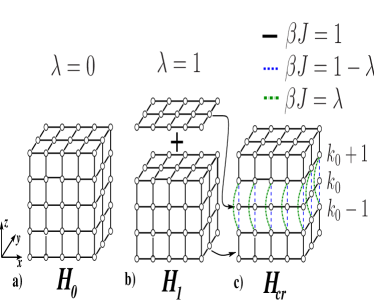
Figure 1: Bond arrangement for the computation of the free energy difference in Eq. (8) (see main text). The crossover Hamiltonian $H_{cr}$ (c) belongs to a system which interpolates between those described by the Hamiltonians $H_{0}$ (a) and $H_{1}$ (b).

If one is interested in the Monte Carlo computation of the difference $F_{1}-F_{0}$ between the free energies $F_{i}=-\frac{1}{\beta}\ln\sum_{{\mathcal{C}}}\exp(-\beta H_{i})$ ($i\in\{0,1\}$) of two lattice models ${\mathcal{M}}_{0}$ and ${\mathcal{M}}_{1}$ with the same configuration space ${\mathcal{C}}$ but different Hamiltonians $H_{0}$ and $H_{1}$, respectively, it is convenient to introduce an “interpolating” system ${\mathcal{M}}_{\rm cr}(\lambda)$ with the crossover Hamiltonian

$$H_{\rm cr}(\lambda)=(1-\lambda)H_{0}+\lambda H_{1},$$ (6)

where $\lambda\in[0,1]$, and again the same configuration space ${\mathcal{C}}$. As a function of the coupling parameter $\lambda$, $H_{\rm cr}(\lambda)$ interpolates between $H_{0}$ and $H_{1}$ as $\lambda$ increases from 0 to 1 and accordingly the free energy $F_{\rm cr}(\lambda)=-\frac{1}{\beta}\ln\sum_{{\mathcal{C}}}\exp(-\beta H_{\rm cr}(\lambda))$ of ${\mathcal{M}}_{\rm cr}(\lambda)$ interpolates between $F_{0}$ and $F_{1}$. The difference $F_{1}-F_{0}$ can be trivially expressed as $F_{1}-F_{0}=\int_{0}^{1}{\rm d}\lambda\,F^{\prime}_{\rm cr}(\lambda)$ where $F^{\prime}_{\rm cr}$ is the derivative of $F_{\rm cr}(\lambda)$ with respect to the coupling parameter:

$$\frac{{\rm d}F_{\rm cr}(\lambda)}{{\rm d}\lambda}=\frac{\sum_{\mathcal{C}}(H_{1}-H_{0}){\rm e}^{-\beta H_{\rm cr}(\lambda)}}{\sum_{\mathcal{C}}{\rm e}^{-\beta H_{\rm cr}(\lambda)}}=\langle\Delta H\rangle_{{\mathcal{M}}_{\rm cr}(\lambda)}\,,$$ (7)

which takes the form of the canonical ensemble average $\langle\ldots\rangle_{{\mathcal{M}}_{\rm cr}(\lambda)}$ of $\Delta H\equiv H_{1}-H_{0}$ and therefore it can be efficiently computed via MC simulations of the lattice model ${\mathcal{M}}_{\rm cr}(\lambda)$. As a result one can conveniently express the difference in free energies as an integral over canonical averages (see, e.g., Ref. Mon ):

$$F_{1}-F_{0}=\int_{0}^{1}\!\!{\rm d}\lambda\,\langle\Delta H\rangle_{{\mathcal{M}}_{\rm cr}(\lambda)}\,.$$ (8)

According to Eq. (5), the Casimir force we are interested in is related to the difference $\Delta F(\beta,L,A)$ between the free energies $F(\beta,L,A)$ and $F(\beta,L-1,A)$ of the same model on two lattices with different numbers of sites and therefore different configuration spaces. In order to apply the method described above for the computation of $\Delta F(\beta,L,A)$ one identifies the model ${\mathcal{M}}_{0}$, its Hamiltonian, and the associated configuration space ${\mathcal{C}}$ with the corresponding ones of the model we are interested in on the lattice $A\times L$, as depicted in Fig. 1(a), so that $F_{0}(\beta,L,A)=F(\beta,L,A)$. The final system ${\mathcal{M}}_{1}$ has to be chosen such that it has the same configuration space ${\mathcal{C}}$ as ${\mathcal{M}}_{0}$. This is achieved by adding to the model on the lattice $A\times(L-1)$ – for which we want to compute the free energy $F(\beta,L-1,A)$ – a two-dimensional lattice of size $A$ with suitable degrees of freedom and lateral periodic BC (see Fig. 1(b)). The Hamiltonian $H_{1}$ of ${\mathcal{M}}_{1}$ is defined such that the added layer does not interact with the remaining part of the system and therefore $F_{1}(\beta,L,A)=F(\beta,L-1,A)+F_{\mathrm{2D}}(\beta,A)$, where $F_{\mathrm{2D}}(\beta,A)$ is the free energy of the isolated two-dimensional layer. This layer can be thought of as the one at position $k_{0}\in\{1,2,\ldots,L\}$ (along the $z$-direction) in the model ${\mathcal{M}}_{0}$ which then decouples from the rest of the lattice upon passing from $\lambda=0$ to $\lambda=1$, i.e., from Fig. 1 (a) to (b). The resulting crossover Hamiltonian $H_{\rm cr}(\lambda)$ (see Eq. (6)) additionally depends on the original position $k_{0}$ of the extracted layer. In particular, in the three-dimensional models we are mainly interested in, the fluctuating degrees of freedom are one- (Ising) or two-component (XY) vectors ${\bf s}_{x,y,z}$ — where $i=(x,y,z)$ specifies the lattice site — which interact only with their nearest neighbors on the same lattice, with a coupling strength $J=1$ (indicated by solid bonds in Figs. 1 (a) and (b); $J$ is absorbed into $\beta$). For them one explicitly finds

$$\begin{split}\Delta H\equiv H_{1}-H_{0}=&-\sum_{x,y}({\bf s}_{x,y,k_{0}-1}\cdot{\bf s}_{x,y,k_{0}+1}\\ -&{\bf s}_{x,y,k_{0}-1}\cdot{\bf s}_{x,y,k_{0}}-{\bf s}_{x,y,k_{0}}\cdot{\bf s}_{x,y,k_{0}+1})\;.\end{split}$$ (9)

The resulting $H_{\rm cr}(\lambda)=H_{0}+\lambda\Delta H$ is characterized by the coupling constants depicted in Fig. 1(c). The free energy difference $\Delta F$ (see Eqs. (5) and (8)) can be finally expressed as

$$\Delta F(\beta,L,A)=-I(\beta,L,A)+F_{\mathrm{2D}}(\beta,A)$$ (10)

where $I(\beta,L,A)=\int_{0}^{1}{\rm d}\lambda\langle\Delta H\rangle_{{\mathcal{M}}_{\rm cr}(\lambda)}$. Note that $H_{\rm cr}(\lambda)$ (see Fig. 1(c)), $\Delta H$ (see Eq. (9)), and therefore $\langle\Delta H\rangle_{H_{\rm cr}(\lambda)}$ depend on the value of $k_{0}$ whereas $I(\beta,L,A)$ is actually independent of it, as long as the boundary conditions are not affected by the extraction of the $k_{0}$-th layer as $\lambda$ varies between 0 and 1. For fixed and open BC in the $z$-direction this requires $k_{0}\neq 1$, whereas for PBC there is no such a restriction on $k_{0}$ and $\langle\Delta H\rangle_{H_{\rm cr}(\lambda)}$ is actually independent of it. In our simulations we have chosen $k_{0}=L/2$.

Once $\Delta F(\beta,L,A)$ has been computed, one has still to subtract $f^{\mathrm{bulk}}(\beta)$ from it (see Eq. (5)), in order to determine the Casimir force in a film of assigned thickness $L-1/2$. However, the accurate computation of the bulk free energy density $f^{\mathrm{bulk}}(\beta)$ is a numerical problem by itself and extracting it from finite-size data requires a very accurate analysis. In order to avoid this complication in the computation of the Casimir force, it is convenient to consider the difference between the forces acting in slabs of thicknesses $L_{1}$ and $L_{2}>L_{1}$:

$$\begin{split}\Delta&\hat{f}_{\mathrm{C}}(\beta,L_{1},L_{2},A)\\ &\equiv\hat{f}_{\mathrm{C}}(\beta,L_{1}-\frac{1}{2},A)-\hat{f}_{\mathrm{C}}(\beta,L_{2}-\frac{1}{2},A)\\ &=\frac{\beta}{A}[I(\beta,L_{1},A)-I(\beta,L_{2},A)]\end{split}$$ (11)

in which the contributions of both $f^{\mathrm{bulk}}(\beta)$ and $F_{\mathrm{2D}}(\beta,A)$ actually cancel. Accordingly, the procedure to calculate the scaling function of the Casimir force consists of the following steps: (1) For a given geometry $L\times A$ and temperature $\beta^{-1}$, via MC simulations we compute the ensemble averages $\langle\Delta H\rangle_{H_{\rm cr}(\lambda)}$ for different values of $\lambda\in\{\lambda_{1},\ldots\lambda_{N}\}$. (2) On the basis of these $N$ values we calculate the integral $I(\beta,L,A)$ in Eq. (8) via numerical integration. (3) These computations are repeated for different sizes $L$, $A$, and temperatures $\beta^{-1}$, yielding numerical estimates for $\Delta\hat{f}_{\mathrm{C}}(\beta,L_{1},L_{2},A)$ (see Eq. (11)). (4) The scaling function $\vartheta$ in Eq. (3) is retrieved from the numerical data for $\Delta\hat{f}_{\mathrm{C}}$ as described below. The results presented in Sec. IV have been obtained by using the Simpson integration method with $N=20$ mentioned above in step (2) and by using pairs of geometries $(L_{1},L_{2})=(L,2L)$ with $L=13,16,20$ for the Ising model and $L=10,15,20$ for the XY model, as introduced in step (4) and for fixed aspect ratios $\rho\equiv L/\sqrt{A}$. (The motivation for our choice $L_{2}=2L$ will be provided in the following subsection.) The method of Ref. hucht takes advantage of the possibly available numerical knowledge of the bulk energy density $u^{\mathrm{bulk}}$ of the model of interest whereas here the analogous information on the bulk free energy $f^{\mathrm{bulk}}$ is not required for the determination of the Casimir scaling function, making our approach applicable also to cases in which there is no detailed knowledge of $u^{\mathrm{bulk}}$ and $f^{\mathrm{bulk}}$.

III.2 Determination of the scaling function

The scaling function $\vartheta$ of the Casimir force can be extracted from the temperature dependence of $\Delta\hat{f}_{\mathrm{C}}(\beta,L_{1},L_{2},A)$, for fixed $L_{1,2}$ and $A$, by using the fact that $\hat{f}_{\mathrm{C}}$ in Eq. (11) scales according to Eq. (3) for large $L_{1,2}$ and $A$. In order to highlight these scaling properties it is convenient to introduce the quantity

$$\begin{split}&g(y;L_{1},L_{2},A)\equiv\left(L_{1}-1/2\right)^{d}\times\\ &\quad\quad\quad\quad\Delta\hat{f}_{\mathrm{C}}(\beta=\beta(y;L_{1}),L_{1},L_{2},A)\,,\end{split}$$ (12)

as a function of $y$, where $\beta(y;L_{1})\equiv\beta_{c}/[1+y(L_{1}-1/2)^{-1/\nu}]$. According to Eq. (3) and with $\tau=(\beta_{c}-\beta)/\beta$, $g$ is expected to scale as

$$g(y;L_{1},L_{2},A)=\hat{\theta}(y)-\alpha^{-d}\hat{\theta}(\alpha^{1/\nu}y)\,,$$ (13)

where $\alpha=(L_{2}-1/2)/(L_{1}-1/2)$ is the width ratio, and $\hat{\theta}(y)$ is the Monte Carlo estimate of $\theta(y)\equiv\vartheta(y/(\xi_{0}^{+})^{1/\nu})$; here $d=3$. Note that, even though $\theta$ is independent of this geometrical realization of the simulation cell, $\hat{\theta}$ might depend on it via $A$ and $L_{1,2}$ due to corrections to scaling. For a given pair of geometries $L_{1}\times A$ and $L_{2}\times A$, the available Monte Carlo data for $\Delta\hat{f}_{\mathrm{C}}(\beta,L_{1},L_{2},A)$ at different temperatures allow one to determine $g(y;L_{1},L_{2},A)$ for a discrete set of values of $y$. In order to determine $\hat{\theta}(y)$ from the numerical data for $g(y;L_{1},L_{2},A)$ with fixed $L_{1,2}$ and $A$, one can solve Eq. (13) iteratively. One can expect (see below) that this yields a solution for $L_{2}>L_{1}$, i.e., $\alpha>1$ together with the property $\hat{\theta}(|y|\rightarrow\infty)\rightarrow 0$ (which holds apart from $T<T_{c}$ in the XY model). As a first approximation of the actual $\hat{\theta}(y)$ one takes $\hat{\theta}_{0}(y)\equiv g(y;L_{1},L_{2},A)$, which can be improved by taking into account that Eq. (13) yields $\hat{\theta}(y)=\hat{\theta}_{0}(y)+\alpha^{-d}\hat{\theta}(\alpha^{1/\nu}y)\simeq\hat{\theta}_{0}(y)+\alpha^{-d}\hat{\theta}_{0}(\alpha^{1/\nu}y)$. Accordingly, a better approximant $\hat{\theta}_{1}(y)$ is provided by

$$\hat{\theta}_{1}(y)=\hat{\theta}_{0}(y)+\alpha^{-d}\hat{\theta}_{0}(\alpha^{1/\nu}y).$$ (14)

The values of $\hat{\theta}_{0}$ at the point $\alpha^{1/\nu}y$, for which no MC data might be available, are obtained by cubic spline interpolation of the available ones. In Eq. (14) one can replace $\hat{\theta}_{0}$ by using Eq. (13), yielding $\hat{\theta}_{1}(y)=\hat{\theta}(y)-\alpha^{-2d}\hat{\theta}(\alpha^{2/\nu}y)\simeq\hat{\theta}(y)-\alpha^{-2d}\hat{\theta}_{1}(\alpha^{2/\nu}y)$, which indicates how the approximant $\hat{\theta}_{1}(y)$ can be improved by introducing $\hat{\theta}_{2}(y)=\hat{\theta}_{1}(y)+\alpha^{-2d}\hat{\theta}_{1}(\alpha^{2/\nu}y)=\hat{\theta}(y)-\alpha^{-4d}\hat{\theta}(\alpha^{4/\nu}y)$. This expression can in turn be used to further improve the approximant along the same lines. The resulting iterative procedure yields a sequence of approximants

$$\hat{\theta}_{k\geq 1}(y)=\hat{\theta}_{k-1}(y)+\alpha^{-2^{k-1}d}\hat{\theta}_{k-1}(\alpha^{2^{k-1}/\nu}y),$$ (15)

which converges very rapidly because the correction to the $k$-th approximant is of the order of $\alpha^{-2^{k-1}d}$, i.e., exponentially small in $2^{k}$ and, in addition, $\hat{\theta}(y)$ is generally expected to decay exponentially for large $|y|$. With $\alpha\simeq 2$, already for $k=5$ one has $\alpha^{-2^{k-1}d}\simeq 3.5\times 10^{-15}$ in three dimensions ($d=3$). The choice of $\alpha\simeq L_{2}/L_{1}$ is a compromise between two competing aims: a small value reduces the sizes of the lattices required for the computation of $\hat{f}_{\mathrm{C}}$ but on the other hand it decreases the accuracy of a given approximant in determining $\hat{\theta}$. With our choice of geometries $(L_{1},L_{2})=(L,2L)$, one has $\alpha\simeq 2$ and a very good approximation of $\hat{\theta}(y)\equiv\hat{\theta}_{k\to\infty}(y)$ is already provided by $\hat{\theta}_{5}(y)$.

III.3 Details of the MC simulations and test of the method

In order to compute the canonical average $\langle\Delta H\rangle_{{\mathcal{M}}_{\rm cr}(\lambda)}$ we use a hybrid MC method which is a suitable mixture of Wolff and Metropolis algorithms LB . Specifically, for the Ising model each hybrid MC step consists of four flips of a Wolff cluster according to the Wolff algorithm, typically followed by $3A$ attempts to flip a spin $s_{x,y,z}$ with $z\in\{k_{0}-1,k_{0},k_{0}+1\}$, which are accepted according to the Metropolis rate LB . An analogous method, with a suitable implementation of Metropolis and Wolff algorithms, has been used for the XY model GH , i.e., a flip of a Wolff cluster according to the Wolff algorithm is typically followed by the implementation of moves according to the Metropolis algorithm  LB .

In order to test the program we have computed numerically $g(y,5,10,9)$ as a function of $y$ for the Ising model on a lattice $3\times 3\times L$ with periodic, $(++)$, and $(+-)$ BC, finding perfect agreement with the result of the analytic calculation based on the transfer-matrix method.

III.4 Corrections to scaling

Finite-size scaling is known to be valid asymptotically for large lattices and small values of $\tau$, i.e., a large correlation length $\xi$ FSS . Away from the asymptotic regime corrections to the leading (universal) scaling behavior become relevant. These non-universal corrections affect both the scaling variables and the scaling functions and depend on the details of the model as well as on the geometry and the boundary conditions privman ; luck . Renormalization-group analyses reveal that there is a whole variety of sources of corrections which arise from bulk, surface, and finite-size effects FSS .

For the limited thicknesses $L$ of the lattices we investigated with our MC simulations it is necessary to take corrections to scaling into account in order to obtain data collapse hucht ; EPL . In the present case, the finite-size scaling variable $\tau(L/\xi_{0}^{+})^{1/\nu}$ (in the following associated with the reduced temperature $\tau$) is expected to acquire a leading correction of the form

$$x\equiv\tau(L/\xi_{0}^{+})^{1/\nu}(1+g_{\omega}L^{-\omega}),$$ (16)

where $\omega$ is the leading correction-to-scaling exponent in the bulk which takes the values $0.84(4)$ and $0.79(2)$ PV for the three-dimensional Ising and XY universality class, respectively. Corrections to the scaling behavior of the critical Casimir force $\hat{f}_{\mathrm{C}}$ are expected to be of the form

$$\begin{split}\hat{f}_{\mathrm{C}}(\beta,L,A)&=L^{-d}\hat{\vartheta}(x,L^{-\omega^{\prime}})\\ &\simeq L^{-d}\vartheta(x)[1+L^{-\omega^{\prime}}\phi(x)+\ldots],\end{split}$$ (17)

for $L\gg 1$, where the exponent $\omega^{\prime}$ controls the leading corrections to the scaling behavior of the lattice estimate $\hat{f}_{\mathrm{C}}$. Its value is determined by that irrelevant surface or bulk perturbation of the Hamiltonian $H$ which has the smallest scaling dimension and which also affects $\hat{f}_{\mathrm{C}}$. In the generic bulk case one has $\omega^{\prime}=\omega$. But its value can be suitably increased (so that the influence of the corrections is reduced) by using improved Hamiltonians and observables, which can also serve as representatives of the same universality class. This is described in detail in Ref. PV . In the presence of surfaces, irrelevant surface perturbations might yield $\omega^{\prime}<\omega$, but we are not aware of either theoretical or numerical studies of this issue. In addition, for small lattice sizes, next-to-leading corrections to scaling might also be of relevance. If $\omega^{\prime}>1/2$, these corrections are generically provided by analytic terms $\sim L^{-1}$ (even though they might be absent in some quantities). The interplay between the leading and next-to-leading corrections (especially if they are sizable) might result in an effective exponent $\omega_{{\rm eff}}$. The current accuracy of our Monte Carlo data and the relatively small range of sizes $L$ investigated here do not allow a reliable determination of $\omega^{\prime}$ and $\phi(x)$. In particular it will turn out that the corrections to scaling are quite well captured by assuming $\phi(x)\simeq g_{2}$, i.e., a constant within the range of the scaling variable we have investigated, and an effective exponent $\omega_{{\rm eff}}$ for the size dependence.

In the discussion of the expected scaling behavior of $\hat{f}_{\mathrm{C}}$ we have assumed that the aspect ratio $\rho\equiv L/\sqrt{A}$ is small enough (i.e., $\rho\ll 1$) so that the scaling behavior in Eq. (3) holds, which formally corresponds to the limit $A\rightarrow\infty$. On the other hand, the actual Monte Carlo simulations have been performed on lattices with small but non-zero $\rho$ and therefore possible additional, $\rho$-dependent corrections have to be taken into account in order to be able to extrapolate our results to the limit $\rho\to 0$. The numerical results in Ref. MN on the (universal) $\rho$-dependence of the Casimir amplitude $\vartheta(0,\rho)$ (see Eq. (3)) of the three-dimensional XY model with periodic and free boundary conditions suggest $\vartheta(0,0)\simeq\vartheta(0,\rho)(1+r\rho^{2})$ for $\rho\lesssim 0.5$, where $r$ is a constant. (This is confirmed also by the analysis in Ref. hucht .) In what follows we assume that this dependence on $\rho$ carries over to the whole scaling function so that $\vartheta(x,0)\simeq\vartheta(x,\rho)(1+\phi_{2}(x)\rho^{2})$. Although the amplitude $\phi_{2}(x)$ of the correction might depend on the scaling variable $x$ (and possibly on $L^{-\omega^{\prime}}$), we shall assume that $\phi_{2}(x)\simeq r_{2}$, i.e., a constant at least within the range of values of the scaling variable $x$ which is studied in the present analysis. On the same footing, we expect a quadratic $\rho$-dependence of the finite-size scaling variable $x(\rho)\simeq x(0)(1+r_{1}\rho^{2})$ associated with the reduced temperature $\tau$, where $r_{1}$ is a constant and $x(0)$ is given by Eq. (16). Taking into account all these corrections, we identify

$$x=\tau\left(\frac{L}{\xi_{0}^{+}}\right)^{\frac{1}{\nu}}(1+g_{\omega}L^{-\omega})(1+r_{1}\rho^{2}),$$ (18)

as the finite-size scaling variable, in terms of which the expected scaling behavior of $\hat{f}_{\mathrm{C}}$ is given by

$$\hat{f}_{\mathrm{C}}(\beta,L,A)=L^{-d}(1+g_{2}L^{-\omega_{{\rm eff}}})(1+r_{2}\rho^{2})^{-1}\vartheta(x).$$ (19)

We shall aim at fixing the non-universal constants $r_{1,2}$, $g_{\omega}$, and $g_{2}$, which generally depend on the boundary conditions, in such a way that the data collapse of the available Monte Carlo data is optimal.

In most of the cases considered below, the accuracy of the data and the range of sizes $L$ investigated do not allow for the reliable determination of both the amplitude $g_{2}$ and the exponent $\omega_{{\rm eff}}$ of the correction. Therefore we fix $\omega_{{\rm eff}}=1\simeq\omega^{\prime}$, which actually leads to a reasonably good data collapse within the considered range of the scaling variable.

In the absence of corresponding dedicated theoretical and numerical analyses, there is no a priori reason why one should prefer the use of a specific form of corrections to scaling, because all of them amount to an effective way of accounting for these corrections. Accordingly, adopting a pragmatic approach, we shall choose that form which leads to the best data collapse or to the best fit. Specifically, we use the following functional forms of corrections to scaling:

$$\begin{split}&\mbox{case (i):}\\ &\hat{f}_{\mathrm{C}}(\beta,L,A)=L^{-d}(1+g_{1}L^{-1})^{-1}(1+r_{2}\rho^{2})^{-1}\hat{\vartheta}\left(x\right),\end{split}$$ (20)

$$\begin{split}&\mbox{case (ii):}\\ &\hat{f}_{\mathrm{C}}(\beta,L,A)=L^{-d}(1+g_{2}L^{-1})(1+r_{2}\rho^{2})^{-1}\hat{\vartheta}(x),\end{split}$$ (21)

$$\begin{split}&\mbox{case (iii):}\qquad\qquad\\ &\hat{f}_{\mathrm{C}}(\beta,L,A)=L^{-d}(1+g_{3}L^{-\omega_{{\rm eff}}})\hat{\vartheta}\left(x\right),\qquad\qquad\end{split}$$ (22)

and

$$\begin{split}&\mbox{case (iv):}\\ &\hat{f}_{\mathrm{C}}(\beta,L,A)=L^{-d}\frac{(1+{\tilde{g}}_{1}L^{-1})}{(1+{\tilde{g}}_{2}L^{-1})}(1+r_{2}\rho^{2})^{-1}\hat{\vartheta}(x).\end{split}$$ (23)

Case (i), (ii), and (iv) become all equivalent for large lattice sizes $L$. On the other hand, for smaller lattice sizes, they lead do different estimates. The coefficients $g_{1},g_{2},g_{3}$ and $\tilde{g}_{1},\tilde{g}_{2}$ are determined in such a way as to optimize the data collapse in the resulting estimate for $\vartheta(x)$ (see below). The factor of the form (iv), with two fitting parameters, will be considered only if data corresponding to several different values of $L$ are available, so that the resulting estimates for $\tilde{g}_{1}$ and $\tilde{g}_{2}$ are reliable. Case (iii) of corrections to scaling works well for the XY and the Ising model with periodic BC. In cases in which corrections to scaling are not small, the ansatz used for their dependence on $L$ might lead to a biased estimate of the scaling function $\vartheta(x)$.

In order to highlight and assess the relevance of the different kinds of corrections, we present in the following sections also the MC data for the function $g(y;L,2L,A)$ which is the primary quantity determined by our MC simulation and from which the scaling function $\hat{\vartheta}(x)$ is eventually obtained according to the procedure described in Subsec. III.2. In the absence of corrections to scaling, data for $g$ (see Eq. (12)) with $L_{2}=2L_{1}$, $L_{1}=L$, as a function of $y=(\beta_{c}/\beta-1)(L-1/2)^{1/\nu}=\tau(L-1/2)^{1/\nu}$ with fixed $\rho=L/\sqrt{A}$ but different sizes $L$ should collapse on a single master curve, which, however, it is not always the case (see, c.f., Fig. 2(a)). In order to account for the corrections to scaling we proceed as follows: First, for fixed values of $L$ and $A=(L/\rho)^{2}$ we determine the Monte Carlo data for $g$ (see Eq. (12)) for different values of the inverse temperature $\beta$. Second, from the plot of $g$ as a function of the rescaled reduced temperature $y=\tau(L-1/2)^{1/\nu}$, i.e., from $g(y;L,2L,A)$, we determine the estimate of the scaling function $\hat{\theta}(y)$, according to the procedure described in Subsec. III.2. This procedure is repeated for the different geometries considered in each case. Because of corrections to scaling and corrections due to $\rho\neq 0$, the resulting estimates $\hat{\theta}(y)$ actually depend on the specific values of $L$ and $A=(L/\rho)^{2}$, i.e., $\hat{\theta}=\hat{\theta}(y;L,\rho)$. In order to extract the asymptotic limit $\theta$ of the scaling function of the Casimir force from the lattice estimate $\hat{\theta}$, we account for corrections in accordance with Eqs. (18) and (19) (with possibly different forms for the $L$-dependent corrections, see Eqs. (LABEL:eq:xy_f_fit1)–(LABEL:eq:fit_new)), which involve several fitting parameters. In those cases in which we apply corrections to scaling due to the aspect ratio dependence of the function $g(y;L,2L,A)$ (which turns out to be the case only for the XY model), the actual fitting procedure we shall use is divided into two steps.

In the first step we fix the value of $L$ ($L=10$ for the XY model) and consider data corresponding to different aspect ratios $\rho$ ($\rho^{-1}=4,5,6,8,10$ for XY). The parameters $r_{1}$ and $r_{2}$ are therefore determined such that the data for $(1+r_{2}\rho^{2})^{-1}\hat{\theta}(y;L,\rho)$ ($\propto\theta(x)$ for fixed $L$) as a function of $y(1+r_{1}\rho^{2})$ ($\propto x$, see Eq. (16), for fixed $L$) yield the best data collapse onto a single curve which ideally corresponds to the scaling function in the limit $A\rightarrow\infty$, but which is still affected by $L$-dependent corrections to scaling. (This procedure actually assumes that, according to Eqs. (18) and (19), $r_{1}$ and $r_{2}$ do not depend on $L$.)

In the second step we fix the value of $\rho$ ($\rho=1/6$ for both XY and Ising) and we determine $g_{\omega}$ and $g_{2}$ (or $g_{1}$ or both ${\tilde{g}}_{1}$ and ${\tilde{g}}_{2}$, depending on the specific form assumed for the corrections) in such a way that the data for $(1+g_{2}L^{-\omega_{{\rm eff}}})\hat{\theta}(y;L,\rho)$ ($\propto\theta(x)$ for fixed $\rho$) as a function of $y(1+g_{\omega}L^{-\omega})$ ($\propto x$, see Eq. (16), for fixed $\rho$) yield the best data collapse onto a single curve. (This procedure actually assumes that, according to Eqs. (18) and (19), in a first approximation corrections to scaling do not depend on $\rho$.) The details of the fitting procedure are described in Appendix A. Our final numerical estimate of the scaling function $\vartheta(x)$ of the Casimir force is then provided by the curve which result from plotting $(1+g_{2}L^{-\omega_{{\rm eff}}})(1+r_{2}\rho^{2})^{-1}\hat{\theta}(y;L,\rho)$ (or equivalent forms as given by the cases (i)-(iv)) as a function of $y(1+g_{\omega}L^{-\omega})(1+r_{1}\rho^{2})/(\xi_{0}^{+})^{1/\nu}\equiv x$, where the fitting parameters have been fixed according to the procedure described above.

Finally it is worthwhile to keep in mind that besides the common corrections to the leading critical behavior in experimental data, the available experimental results for critical Casimir forces contain an additional source of corrections in that the thickness $L$ of the (wetting) films is definition-dependent up to a microscopic length $\ell_{0}$ DSD:07 . Accordingly, only the leading term is universal whereas the correction $\sim\ell_{0}/L$ is even definition-dependent. Moreover, also the relation between the experimental values $L_{\rm exp}$ and the theoretical values $L_{\rm theo}$ suffers from the same kind of uncertainty.

IV Results

In this section we summarize the numerical results for the scaling function of the critical Casimir force within the three-dimensional XY (Subsec. IV.1) and Ising (Subsec. IV.2) universality classes with different boundary conditions. As mentioned in the Introduction, the former are relevant for the interpretation of the experiments with wetting films of ⁴He garcia , whereas the latter apply to the case of classical binary mixtures pershan ; Hertlein . In most of the presented plots the size of the symbols are of the order of the statistical error. In these cases the corresponding error bars are not shown in the figures.

IV.1 XY model

For the simulations of the XY model we have considered films of thicknesses $L=10,15$, and $20$, and transverse areas $A=L_{x}\times L_{y}=6L\times 6L$ corresponding to an aspect ratio $\rho=L/\sqrt{A}=1/6$. At the boundaries in the $x$- and $y$-directions we impose periodic BC, whereas in the $z$-direction we consider either free surface spins, corresponding to the $(O,O)$ universality class, or periodic BC.

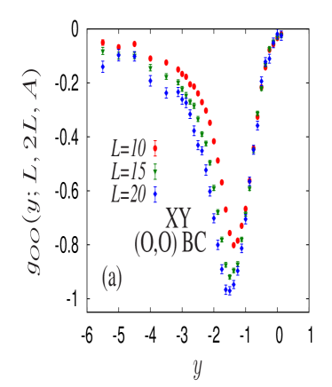
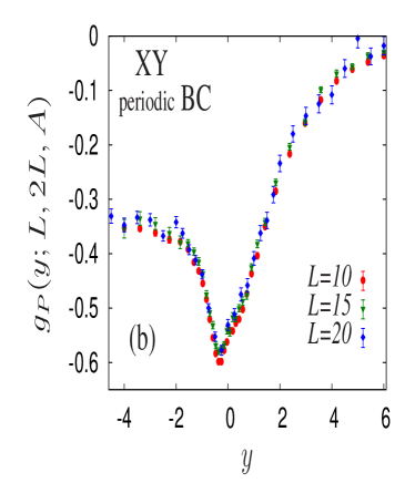
Figure 2: Monte Carlo data for $g(y=\tau(L-\frac{1}{2})^{1/\nu};L,2L,A=(L/\rho)^{2})$ (see Eq. (12), $\tau=(T-T_{c})/T_{c}$) in the three-dimensional XY model for $L=10$, $15$, $20$, and fixed inverse aspect ratio $\rho^{-1}=6$. In (a) and (b) we present the result for $(O,O)$ and periodic BC, respectively. For $T\geq T_{c}$, i.e., $y=y_{+}>0$ one has $y_{+}=[(L-\frac{1}{2})\xi^{+}_{0}/\xi_{+}]^{1/\nu}$. For the XY model $\xi_{-}=\infty$ for all temperatures $T\leq T_{c}$. The Kosterlitz-Thouless transition of the two-dimensional film occurs at $y=y_{c,OO}=-2.69(3)$ Hasen and $y=y_{c,P}=-0.996(1)$ SM-95 in (a) and (b), respectively.

In Fig. 2 we report the data corresponding to $g(y;L,2L,A)$ (see Eq. (12)) for (a) $(O,O)$ and (b) periodic BC. Corrections to scaling, which are signaled by the fact that data corresponding to different $L$ do not fall onto the same master curve, are much more pronounced for the case of $(O,O)$ BC (see Fig. 2(a)) as compared with the case of periodic BC (see Fig. 2(b)). The same holds for the dependence of the data on the aspect ratio $\rho$ (data for $(O,O)$ are not shown, data for periodic BC are presented in Fig. 3). For $(O,O)$ and periodic BC corrections to scaling are more relevant for $y\lesssim y_{\rm min}$, where $y_{\rm min}$ is the value of $y$ at which the function $g(y;L,2L,A)$ attains its minimum. For $y\gtrsim y_{\rm min}$ the data obtained for different $L$ follow a common curve. We note that the bulk correlation length $\xi$ of the XY model is infinite for all temperatures below $T_{c}$: $\xi(T\leq T_{c})=\infty$. Accordingly, within the XY model the scaling variable $y$ can be expressed as $y=[(L-1/2)\xi_{0}^{+}/\xi]^{1/\nu}$ only for $T\geq T_{c}$.

Interestingly, for both types of BC the aspect ratio dependence is particularly strong in the range of temperatures around the minimum of the function $g(y;L,2L,A)$, i.e., $-2\lesssim y\lesssim-1$ and $-1\lesssim y\lesssim 0$ for $(O,O)$ and periodic BC, respectively (see Fig. 3). According to Fig. 2, the minimum of $g(y;L,2L,A)$ for periodic BC occurs at the reduced temperature $\tau_{\rm min}=-y_{\rm min}/(L-\frac{1}{2})^{1/\nu}\simeq-0.31/(L-\frac{1}{2})^{1/\nu}$. For $(O,O)$ BC it occurs slightly further away from $T_{c}$, i.e., at $y_{\rm min}\simeq-1.34$ and $-1.50(3)$, depending on the value of $L$. We find that changing $L$ at a fixed aspect ratio results in slight relative shifts of the data whereas changing $\rho$ at fixed $L$ leads to much more pronounced differences (see Fig. 3). This behavior is expected to be related to the finite-size effects near the thin film critical point. Within the Ising model, for an infinitely large transverse area $A$ the point at which the film with $(O,O)$ or periodic BC exhibits the 2D critical behavior is located on the bulk coexistence line $H=0$ at a size-dependent temperature $T_{c}(L)<T_{c}$ such that $\xi(T=T_{c}(L))\sim L$. Accordingly, upon increasing $L$, $T_{c}(L)$ approaches the three-dimensional bulk value $T_{c}$ as $T_{c}(L\rightarrow\infty)=T_{c}(1+y_{c}L^{-1/\nu})$ FSS , where $y_{c}$ is negative, non-universal, and depends, inter alia, on the type of BC. The corresponding scaling variable $x(L)\equiv[(T_{c}(L)-T_{c})/T_{c}](L/\xi_{0}^{+})^{1/\nu}$ tends to a universal and BC-dependent value $x^{*}\equiv x(L\rightarrow\infty)=y_{c}(\xi_{0}^{+})^{-1/\nu}$. Hence, $y_{c}$ is expected to lie in the vicinity of the minimum of the function $g(y;L,2L,A)$. Accordingly, around its minimum the function $g(y;L,2L,A)$ should exhibit a strong dependence on the aspect ratio $\rho$ if the bulk correlation length $\xi^{\mathrm{2D}}$, associated with the shifted critical point of the two-dimensional film ES , becomes comparable with the characteristic transverse length $L_{\parallel}\equiv\sqrt{A}$ of the simulated system.

Figure 3: Monte Carlo data for $g(y=\tau(L-\frac{1}{2})^{1/\nu};L,2L,A=(L/\rho)^{2})$ (see Eq. (12), $\tau=(T-T_{c})/T_{c}$) within the three-dimensional XY model with periodic BC for $L=10$ and different values of the inverse aspect ratio $\rho^{-1}$. For $y\geq 0$ one has $y=y_{+}=[(L-\frac{1}{2})\xi_{0}^{+}/\xi_{+}]^{1/\nu}$. For the XY model $\xi_{-}=\infty$ for all temperatures $T\leq T_{c}$. The Kosterlitz-Thouless transition of the two-dimensional film occurs at $y=y_{c,P}=-0.996(1)$ SM-95 . Note the enlarged scales as compared with Fig. 2(b).

Within the XY model the critical point of the thin film belongs to the Kosterlitz-Thouless (KT) universality class K-T . The KT theory predicts that upon approaching this critical point from the high temperature phase the correlation length $\xi_{KT}\sim\exp[(1-\beta/\beta_{c}^{KT})^{-\nu^{KT}}]$, $\nu^{KT}=1/2$, diverges exponentially. The shift of $T_{c}(L)$ relative to the bulk critical point is expected to scale with the film thickness $L$ in the same way as for the Ising model, i.e., $(T_{c}(L)-T_{c})/T_{c}\simeq y_{c}L^{-1/\nu}$ for large $L$, with $\nu=0.662(7)$ for the 3D XY model. This prediction is in agreement with MC simulations of various models belonging to the XY universality class and confined in films with free janke ; SS-92 ; Hasen or periodic SM-95 BC. The critical exponent $\nu$ obtained from early simulations janke ; SS-92 of films with free BC was slightly larger ($\nu\simeq 0.7$ janke ; SS-92 ) than the theoretically predicted value $\nu=0.662(7)$, due to rather strong corrections to scaling which need to be taken into account in order to observe the theoretically expected behavior Hasen . The results of Ref. Hasen for $x^{*}_{OO}=-7.64(15)$ yield the estimate $y_{c,OO}=-(\xi_{0}^{+})^{1/\nu}x^{*}_{OO}=-2.69(3)$ for the location of the shifted KT transition in the XY model with free boundary conditions, whereas $y_{c,P}=-0.996(1)$ for PBC SM-95 . It turns out that in the simulations with free BC janke the positions of the maxima of the thermodynamic functions such as the peak of the specific heat or the peak of the susceptibility do not coincide with the transition point but occur at ca. $1.3\times T_{c}(L)$. (These quantities are not related to singularities of XY films.) With increasing film thickness $L$ the absolute distance in temperature of these peaks from $T_{c}(L)$ decreases and for $L=10$ the simulations of Ref. janke report a shift of less than 10$\%$. There is also experimental evidence that as a function of temperature the position of the minimum of the Casimir force of ⁴He films, which belong to the universality class of XY films, coincides with the position $T_{m}(L)$ of their specific heat maximum (see Subsec. VD and Figs. 21 and 32 in Ref. gasparini ), whereas the onset of superfluidity in these films occurs at $T_{c}(L)<T_{m}(L)$ (see Subsec. VD and Figs. 24, 32, and 33 in Ref. gasparini ). A similar behavior may be expected to hold for the function $g(y;L,2L,A)$. Indeed, as can be seen from Figs. 2 and 3, the minima of the function $g(y;L,2L,A)$ lie in the vicinity of the corresponding values of $y_{c}$. Therefore, similar to the Ising model, the strong aspect ratio dependence around the minimum might occur when the exponentially diverging bulk correlation length $\xi^{\mathrm{2D}}$, associated with the KT critical point of the film, becomes comparable with the characteristic transverse length $L_{\parallel}\equiv\sqrt{A}$ of the simulated system.

IV.1.1 Dirichlet-Dirichlet boundary conditions

We consider first the case of $(O,O)$ BC. As evidenced by Fig. 2(a), in order to achieve a good data collapse of the curves corresponding to different lattice sizes we have to account for corrections to scaling according to Eqs. (18) and (19). As a phenomenological ansatz for the effective corrections we take $\omega_{{\rm eff}}=1$ and consider two functional forms for the $L$-dependent corrections to the scaling function: case (i) [Eq. (LABEL:eq:xy_f_fit1)] and case (ii) [Eq. (LABEL:eq:xy_f_fit2)] as discussed in Subsec. III.4. As a result of the fitting procedure, in the interval $x\in[-6,-2.1]$ (see Eq. (18)) we find $r_{1}=1.18(10)$, $r_{2}=2.40(13)$, $g_{1}=5.83(25)$, and $g_{\omega}=2.25(15)$ in case (i) and $g_{2}=-2.98(8)$ in case (ii) with the same values for $r_{1}$, $r_{2}$, and $g_{\omega}$ as in case (i). Figure 4 shows the corresponding resulting estimates of the scaling function $\vartheta(x)$ of the critical Casimir force. The quality of the data collapse for the two cases separately clearly indicates that Eqs. (LABEL:eq:xy_f_fit1), (LABEL:eq:xy_f_fit2), and (18) are very effective ways of accounting for the corrections to scaling in this system. We find that $\vartheta(x)$ is slightly affected by the choice of the functional form of corrections to scaling and indeed in the two cases one finds estimates of $\vartheta(x)$ which have the same shape but the overall amplitude is reduced by a factor $R\simeq 0.9$ in case (ii) as compared with case (i). The dashed line represents the scaling function which has been determined in Ref. hucht on the basis of a different numerical method and assuming corrections to scaling of the form (i). Even though this result is actually biased by that particular choice (a point which has not been discussed in Ref. hucht ), the very good agreement between the different approaches provides a highly welcome independent test of both methods.

Our MC results for $\vartheta(x)$ compare well also with the experimental data of Ref. garcia . (For a meaningful comparison between the numerical and the experimental scaling function, the abscissa $\tau L^{1/\nu}$ of the experimental data presented in Ref. garcia has to be properly normalized as $\tau(L/\xi_{0}^{+\mathrm{(exp)}})^{1/\nu}$ by using the experimental value $\xi_{0}^{+\mathrm{(exp)}}=1.432$Å ahlers ; footnote .) In particular, the position of the pronounced minimum of the scaling function is properly captured. The corrections to scaling of form (i) yield $x^{(i)}_{\mathrm{min}}=-5.43(2)$ and $\vartheta^{(i)}_{\mathrm{min}}\equiv\vartheta(x^{(i)}_{\mathrm{min}})=-1.396(6)$, whereas those of form (ii) result in $x^{(ii)}_{\mathrm{min}}=-5.43(2)$ and $\vartheta^{(ii)}_{\mathrm{min}}\equiv\vartheta(x^{(ii)}_{\mathrm{min}})=-1.260(5)$. The corresponding experimental values are $x_{\mathrm{min}}^{\mathrm{(exp)}}=-5.7(5)$ and $\vartheta_{\mathrm{min}}^{\mathrm{(exp)}}=-1.30(3)$. Taking into account the aforementioned bias affecting the results of Ref. hucht and the sensitivity of the resulting scaling function to the assumed form of the corrections to scaling we conclude that our estimates for $x_{\mathrm{min}}$ and $\vartheta_{\mathrm{min}}$ are compatible also with those presented there ($-5.3(1)$ and $-1.35(3)$, respectively). As expected, due to the presence of the Goldstone modes below $T_{c}$, both the experimental and the MC data do not approach zero for $x\rightarrow-\infty$ but saturate at some finite negative value at low temperatures. However, the absolute value of the saturation as obtained from the MC simulations is smaller than the experimental one. This difference, which extends deep into the non-critical regime, is, inter alia, due to ⁴He specific properties and to the occurrence of capillary waves on the liquid-vapor interface of the critical ⁴He wetting films. This point has been discussed in Ref. kardar:04 . In Fig. 4 the gray vertical bar indicates the universal value $x^{*}_{O,O}=-7.64(15)$ of the scaling variable corresponding to the occurrence of the Kosterlitz-Thouless transition at $T=T_{c}(L)$ in the film, as inferred from MC simulations of lattice models in the XY universality class presented in Ref. Hasen . The Kosterlitz-Thouless transition is accompanied by an actually invisible essential singularity $\sim\exp(-{\rm const}/\sqrt{|x-x^{*}|})$ in the behavior of the specific heat which, as discussed above, displays a pronounced maximum at a temperature $T=T_{m}(L)$. Accordingly, one does not expect to find any particular signature of this transition in the scaling function of the Casimir force for $x\simeq x^{*}$, in distinction to the case of the Ising model (c.f., Subsecs. IV.2.2 and IV.2.3).

Finally, for completeness, in Fig. 4 we have also included (dash-dotted line) our mean field result for the Casimir scaling function $\vartheta_{OO}^{\mathrm{(MFT)}}$ obtained from the limiting case of the vectoralized Blume-Emery-Griffiths lattice model corresponding to the model of pure ⁴He LGW-MF . The scaling function is normalized to the depth of the minimum of the MC data. For large $L$, $\vartheta_{OO}^{\mathrm{(MFT)}}$ agrees very well with the ones obtained from the $O(2)$ Landau-Ginzburg continuum theory LGW-MF ; LGW-MF1 .

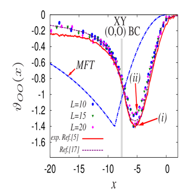
Figure 4: Scaling function $\vartheta_{OO}$ of the Casimir force for the three-dimensional XY model with $(O,O)$ BC. The MC data reported in this figure refer to lattices with $L=10$, $15$, and $20$, with fixed inverse aspect ratio $1/\rho=6$. Corrections to scaling have been accounted for according to two different ansätze, provided by Eq. (LABEL:eq:xy_f_fit1) and Eq. (LABEL:eq:xy_f_fit2); the corresponding numerical results are denoted by (i) and (ii), respectively. With corrections to scaling of the form (ii), the shape of the resulting scaling function is almost indistinguishable from the one obtained with corrections to scaling of the form (i), but its overall amplitude is reduced by a factor $R\simeq 0.9$. For (i) our MC data compare very well with the corresponding experimental data from Ref. garcia (solid line) and with the MC data of Ref. hucht (dashed). Due to the Goldstone modes $\vartheta_{OO}(x\to-\infty)=\mathrm{const}\neq 0$. The dash-dotted line shows the mean field scaling function LGW-MF ; LGW-MF1 normalized to the depth of the minimum of the MC data (i). The levelling off of the experimental data garcia for $x\to-\infty$ contains a component which is specific for ⁴He wetting films kardar:04 and cannot be captured by an XY lattice model. The gray bar indicates the position and uncertainty of the universal value $x^{*}_{O,O}=-7.64(15)$ of the scaling variable $x$ corresponding to the occurrence of the Kosterlitz-Thouless transition in the film, as inferred from MC simulations of lattice models in the XY universality class presented in Ref. Hasen .

IV.1.2 Periodic boundary conditions

In this subsection we discuss the XY model with periodic BC. According to Fig. 2(b) corrections to scaling are much less pronounced in this case than for $(O,O)$ BC (Fig. 2(a)), suggesting that the exponent $\omega_{{\rm eff}}$ might be actually larger than $1$. In addition, the dependence of the numerical data on the aspect ratio $\rho$ turns out to be relevant only in the restricted range $-1\lesssim y\lesssim 0$ of the scaling variable (see Fig. 3), so that the assumed forms of the aspect ratio corrections in Eqs. (18) and (19) do not work best. In the present case, the accuracy of our Monte Carlo data allows us to study in some detail also the Casimir amplitude $\Delta\equiv\vartheta(0)/2$. Upon focusing on such a quantity in a broader range of geometries $(6\leq L\leq 20)$ it turns out that for this amplitude the corrections to scaling are not properly accounted for by the previous ansätze (case (i) and case (ii), Eqs. (LABEL:eq:xy_f_fit1) and (LABEL:eq:xy_f_fit2), respectively). We have therefore tried also a fit of the exponent $\omega_{{\rm eff}}$ according to Eq. (19) with $r_{1,2}=0$ (case (iii), Eq. (LABEL:eq:xy_f_fit3)), which yields for the Casimir amplitude

$$\Delta(L)=\Delta(1+g_{3}L^{-\omega_{{\rm eff}}}).$$ (24)

With this ansatz, our data for $\Delta_{P}(L)$ are very well fitted for $\omega_{{\rm eff}}=2.59(4)$ and $g_{3}=14.9(7)$ in the interval $0\leq L^{-1}\leq 0.15$. (At present, the origin of this rather large value of $\omega_{{\rm eff}}$ is not clear.) The comparison between the numerical data and the fit is reported in Fig. 5. The value of the Casimir amplitude extrapolated to the scaling limit $L\rightarrow\infty$ is $\Delta_{P}(\infty)\equiv\Delta_{P}=-0.2993(7)$ which is slightly smaller than the previous estimate $\Delta_{P}=-0.28$ (see Ref. DK and the discussion below). Note, however, that our estimate is biased by the particular form Eq. (24) assumed for the corrections to scaling.

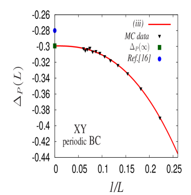
Figure 5: Critical Casimir amplitude $\Delta_{P}(L)$ for the three-dimensional XY bulk universality class and periodic BC, estimated from lattices of several thicknesses $L$ and inverse aspect ratio $1/\rho=6$. Due to corrections to scaling, $\Delta_{P}$ depends on $L$. The solid line represent the best fit to the numerical data based on Eq. (24) and allows one to extrapolate the value of $\Delta_{P}(L)$ to the scaling limit $L\rightarrow\infty$, resulting in $\Delta_{P}=-0.2993(7)$ ($\blacksquare$). With $\bullet$ we indicate the numerical estimate $\Delta_{P}=-0.28$ provided in Ref. DK .

The analysis of the Casimir amplitude $\Delta_{P}(L)$ suggests that the corrections to scaling for periodic BC are well captured (in the range of sizes and of the scaling variable investigated here) by Eq. (LABEL:eq:xy_f_fit3) (case (iii)) and Eq. (18) with $r_{1}=0$. The resulting estimate for the scaling function $\vartheta_{P}$ is reported in Fig. 6 for which we adopt the values for $g_{3}$ and $\omega_{{\rm eff}}$ which we determined from the analysis of the correction to scaling for $\Delta_{P}(L)$. It turns out that a very good data collapse is achieved even without correcting the abscissa, i.e., with $g_{\omega}\simeq 0$, $r_{1}\simeq 0$, within the range of the scaling variable $x$ we have investigated, which actually includes the interval $-1<y<0$ in which the corresponding function $g$ shows a more pronounced dependence on $\rho$.

As another valuable test of the method, our results are compared with the corresponding MC simulation data obtained previously in Ref. DK within a different approach, i.e., by computing the average value of the lattice stress-tensor. In Fig. 6 we report the data set corresponding to the lattice size $L=20$ investigated therein. The shapes of the two scaling functions are very similar but the data points from Ref. DK are shifted upwards with respect to the ones we have obtained. This discrepancy might be due to the uncertainty in the normalization factor used in Ref. DK , where the vertical scale of the data for $\vartheta_{P}$ has to be adjusted on the basis of an independent estimate. This estimate has been obtained from the $\epsilon=4-d$-expansion of the ratio $\Delta_{P,n}/\Delta_{P,1}$ of the Casimir amplitudes for $O(n)$ models with the result $\Delta_{P,n=2}=-0.28$ so that $\vartheta_{P}(0)\equiv 2\Delta_{P,n=2}=-0.56$. In contrast, the method presented here provides absolute values of the amplitude and the scaling function. In addition to the uncertainty concerning the normalization factor, in Ref. DK no corrections to scaling have been applied in the determination of $\vartheta_{P}$. The present MC results provide the estimates $x_{\mathrm{min}}=-0.73(1)$ and $\vartheta_{P}(x_{\mathrm{min}})=-0.633(1)$ characterizing the position of the minimum of the scaling function.

For the scaling function of the XY model with periodic BC some analytical predictions are also available; for a thorough comparison of the scaling function obtained within various approaches see Ref. DKD . Here we discuss only the comparison with the recent results based on a suitable perturbation theory for the $O(n)$ model in a film geometry with periodic BC DGS ; GD , which improves previous analyses krech:92 ; KD-92 of this scaling function for $T\geq T_{c}$ by taking into account a higher-order contribution to the perturbation theory which involves fractional powers of $\epsilon$. In the case $n=2$ (XY model) and in agreement with our MC data this latter analytically available scaling function decreases monotonically for $x\rightarrow 0$ and thus allows for the formation of a minimum below $T_{c}$ (without being able to reach it) whereas the previously available analytic scaling function exhibits a minimum above $T_{c}$. The analytically estimated value for the critical Casimir amplitude is $\Delta_{P}\simeq-0.43$ (i.e., $\vartheta_{P}(0)\simeq-0.86$) which in absolute value is larger than the MC result. In Fig. 6 this analytically predicted scaling function is reported, for comparison, as a solid line.

As already mentioned above, one characteristic feature of the scaling function of the critical Casimir force in the XY model (and, more generally, in systems with continuous symmetry) is its saturation at a nonzero negative value $\vartheta(x\rightarrow\infty)<0$ at low temperatures, which occurs for all non-symmetry breaking BC. This is due to the fact that, even well below the critical temperature, the fluctuations of the order parameter exhibit long-ranged correlations due to the Goldstone modes associated with the broken continuous symmetry, which result in a non-vanishing long-ranged Casimir force. For periodic BC the saturation value $\vartheta_{P}(-\infty)$ is significantly more negative and is approached more rapidly than in the case of $(O,O)$ BC. The line of arguments presented in Ref. kardar:04 for the theoretical calculation (TH) of $\vartheta^{\mathrm{(TH)}}_{O,O}(-\infty)=-\zeta(3)/(8\pi)\simeq-0.049$ (disregarding additional helium-specific surface fluctuations) can be extended to the present case by considering periodic (instead of Neumann as in Ref. kardar:04 ) BC for the fluctuations of the phase field of the order parameter in the film. In three dimensions this yields

$$\vartheta^{\mathrm{(TH)}}_{P}(-\infty)=2\Delta^{\mathrm{(G)}}_{P}\simeq-0.38,$$ (25)

where $\Delta^{\mathrm{(G)}}_{P}=-\zeta(3)/(2\pi)\simeq-0.19$ is the Casimir amplitude for a one-component ($N=1$) fluctuating Gaussian field in a film with PBC (see, e.g., Eq. (9.2) in Ref. KD-92 ), so that $\vartheta^{\mathrm{(TH)}}_{P}(-\infty)/\vartheta^{\mathrm{(TH)}}_{O,O}(-\infty)=8$. The numerical data corresponding to the MC simulations presented in Fig. 6 yield $\vartheta_{P}(-\infty)=-0.383(4)$ (obtained by fitting the data points in the region $-14<x\leq-10$, two of which are actually not shown in Fig. 6, with a constant). This is in very good agreement with the theoretical prediction $\vartheta^{\mathrm{(TH)}}_{P}(-\infty)$ in Eq. (25). Note that the MC data of Ref. DK give $\vartheta_{P}(-\infty)\simeq-0.33$, a value which is biased by the choice of the normalization of the scaling function, as mentioned before. We point out, however, that the line of arguments in Ref. kardar:04 assumes that, deep in the low-temperature phase, the phase field obeys Neumann BC and that the magnitude of the complex order parameter (superfluid density) is spatially constant across the film, i.e., that the effects of the surfaces are effectively negligible. This might not be the case in the presence of the Goldstone modes which can cause the magnitude of the order parameter vary algebraically within the film.

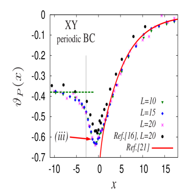
Figure 6: Scaling function $\vartheta_{P}$ of the Casimir force for the three-dimensional XY model with periodic BC. The corrections to scaling are taken into account by Eq. (LABEL:eq:xy_f_fit3) (case (iii)) and Eq.  (18) with $r_{1}=0$. The shape of our MC data compares very well with the corresponding MC data ($\bullet$) of Ref. DK . For a discussion of the relative shift of the data sets see the main text. The solid line corresponds to the analytical prediction in Ref. GD . Due to the Goldstone modes, in agreement with Eq. (25), $\vartheta_{P}(x\to-\infty)=-0.383(4)$, see horizontal dashed line. Contrary to $(O,O)$ BC in Fig. 4, for periodic BC MFT yields $\vartheta_{P}^{\mathrm{(MFT)}}(x)\equiv 0$ for $x\lessgtr 0$. The gray vertical line indicates the position of the universal value $x^{*}_{P}=-2.82(2)$ of the scaling variable $x$ corresponding to the occurrence of the Kosterlitz-Thouless transition in the film, as inferred from MC simulations SM-95 .

Finally, in Fig. 6 we report as a gray vertical line the universal value $x^{*}_{P}=-2.82(2)$ of the scaling variable $x$ corresponding to the occurrence of the Kosterlitz-Thouless transition in the film, as inferred from the MC simulations of the XY model in a film with PBC SM-95 . As in the case of $(O,O)$ BC, there is no singularity possibly visible in $\vartheta_{P}(x)$ associated with this transition.

IV.2 Ising model

In the case of the Ising model we have determined the scaling function $\vartheta$ for $(+-)$, $(++)$, Dirichlet-Dirichlet $(O,O)$, and periodic BC. The first two BC are relevant for interpreting the results of the experiments in Refs. Hertlein ; pershan which use as a critical medium classical binary liquid mixtures near their demixing point.

In our simulations we have used lattices with $L=10$, $13$, $16$, and $20$ and with $L_{x}=L_{y}=6L$, i.e., $\rho=1/6$. Each data point has been averaged over at least $10^{5}$ hybrid MC steps.

Figure 7: Plot of $g(y;L,2L,A=(L/\rho)^{2})$ (see Eq. (12)) for the three-dimensional Ising model with $L=10$ and $1/\rho=6$, $10$, and $14$. (a) and (b) refer to $(++)$ and $(+-)$ BC, respectively, and the coincidence of data points corresponding to different values of $\rho$ demonstrates that the geometry of the lattice does not affect the resulting finite-size critical behavior in the region $-4\lesssim y\lesssim 10$.

IV.2.1 $(++)$ and $(+-)$ boundary conditions

We first discuss the cases of $(++)$ and $(+-)$ BC, for which we find that in the critical regime the numerical data for the function $g(y;L,2L,A)$ are practically independent of the aspect ratio $\rho=L/\sqrt{A}$ (see Fig. 7). The presented data correspond to $L=10$ and to inverse aspect ratios $\rho^{-1}=6,10,14$. In the case of $(+-)$ BC the aspect ratio becomes relevant for $y\lesssim-4$, where the behavior of the system is dominated by the presence of the strongly fluctuating interface which separates the regions with predominantly positive and negative magnetization. The extent of these fluctuations is known to be particularly sensitive to the spatial extension and to the geometry of the system in the directions parallel to the interface (i.e., in the $L_{x}$ and $L_{y}$ directions); therefore the aspect ratio $\rho$ plays an important role for these fluctuations. In $d=3$ one expects a strongly increasing parallel correlation length $\xi_{\parallel}$ which governs the decay of the correlations in the direction parallel to the interface, i.e., $\xi_{\parallel}\sim\exp(L_{\parallel}/(4\xi))$ with $L_{\parallel}=L_{x}=L_{y}$ parryevans . In addition, these strong interfacial fluctuations cause the scaling function $\vartheta_{+-}$ to decay to zero for $x\rightarrow-\infty$ much more slowly than the scaling function $\vartheta_{++}$ (see, c.f., Figs. 10 and 9).

Contrary to the aspect ratio, $L$-dependent corrections to scaling are rather important for the Ising model with $(++)$ and $(+-)$ BC. By using the phenomenological ansätze in Eqs. (18) and (LABEL:eq:xy_f_fit1) or (LABEL:eq:xy_f_fit2) with $r_{1,2}=0$ (which account for the negligible dependence of the data on $\rho$) we have obtained a good data collapse for the scaling functions calculated for $L=13$, $16$, and $20$. However, these ansätze fail to describe the data for the critical Casimir amplitude $\Delta$ in the broader range of thicknesses $6\leq L\leq 20$, as it is the case of the XY model with periodic BC.

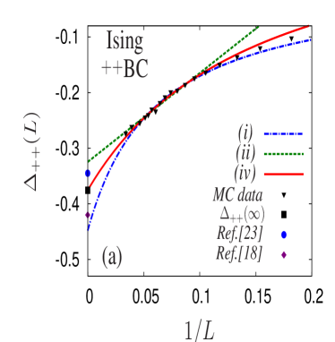
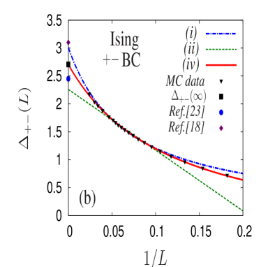
Figure 8: MC data for the critical Casimir amplitude $\Delta(L)$ of the three-dimensional Ising model with (a) $(++)$ and (b) $(+-)$ BC, as a function of the inverse lattice size $L$ (for lattices with fixed inverse aspect ratio $1/\rho=6$). $L$-dependent corrections to scaling give rise to the dependence $\Delta(L)$ such that $\Delta_{++/+-}\equiv\Delta_{++/+-}(L\to\infty)$. The solid line corresponds to the best fit obtained by using the fitting ansatz in Eq. (26) in the interval $0<1/L\leq 0.1$. For comparison we present also the best fits using the ansätze (i) $\Delta(L)=\Delta(1+g_{1}L^{-1})^{-1}$ and (ii) $\Delta(L)=\Delta(1+g_{2}L^{-1})$. Our estimates ($\blacksquare$) for the asymptotic values of the Casimir amplitudes compare reasonably well with previous MC results ($\bullet$) from Ref. krech and with results ($\blacklozenge$) obtained from the de Gennes-Fisher local-functional upton .

It turns out that the corrections to scaling in this range are very well captured by the functional dependence (iv) (Eq. (LABEL:eq:fit_new) introduced in Subsec. III.4, with $r_{1,2}=0$) which for the critical Casimir amplitude yields

$$\Delta(L)=\Delta\frac{(1+\tilde{g}_{1}L^{-1})}{(1+{\tilde{g}}_{2}L^{-1})}.$$ (26)

As in the case of the XY model with periodic BC we shall determine the parameters $\tilde{g}_{1}$ and $\tilde{g}_{2}$ (according to Subsec. III.4) for both $(++)$ and $(+-)$ BC on the basis of the analysis of the corrections to scaling to the corresponding Casimir amplitude and then these values are employed in order to calculate the scaling functions $\vartheta_{++}$ and $\vartheta_{+-}$.

In Figure 8 we present numerical data for $\Delta$ as a function of $1/L$ for both $(++)$ (a) and $(+-)$ (b) BC with the corresponding fit carried out according to Eq. (26) in the interval $0\leq 1/L\leq 0.1$. Other variants of the fit function (within the same fit interval), such as $\Delta(1+g_{1}L^{-1})^{-1}$ and $\Delta(1+g_{2}L^{-1})$, indicated as (i) and (ii), respectively, are also presented for comparison.

For $(++)$ BC the fitting parameters are $\tilde{g}_{1}=-2.6(1.2)$, $\tilde{g}_{2}=6.6(3.7)$ and the resulting estimate for the Casimir amplitude is $\Delta_{++}(L\to\infty)\equiv\Delta_{++}=-0.376(29)$, i.e., $\vartheta_{++}(0)=-0.75(6)$, which compares quite well with the previous MC result $\vartheta_{++}(0)=-0.690(32)$ krech shown as a full circle in Fig. 8(a); for the latter result corrections to scaling were not taken into account. Field-theoretical predictions $\vartheta_{++}^{\mathrm{(FT)}}(0)=-0.652\ldots-0.346$ give numbers slightly smaller in absolute value which depend on the approximant used to re-sum the field-theoretical $\epsilon=4-d$-expansion up to $O(\epsilon)$ series (see Ref. krech for details).

For $(+-)$ BC we have found $\tilde{g}_{1}=-1.8(1)$, $\tilde{g}_{2}=8.54(43)$ and we estimate $\Delta_{+-}(L\to\infty)\equiv\Delta_{+-}=2.71(2)$, i.e., $\vartheta_{+-}(0)=5.42(4)$, in agreement with the experimental value $\vartheta^{\mathrm{(exp)}}_{+-}(0)=6(2)$ pershan but slightly larger compared to the previous MC estimate $\vartheta_{+-}(0)=4.900(64)$ krech (indicated as a full circle in Fig. 8(b), still affected by finite-size corrections) and the analytical estimates $\vartheta_{+-}^{\mathrm{(FT)}}(0)=3.16\ldots 4.78$. The latter depend on the approximant used to re-sum the $O(\epsilon)$ series (see Ref. krech for details).

By using the values of $\tilde{g}_{1}$ and $\tilde{g}_{2}$ obtained previously in the context of the Casimir amplitude we determine the coefficient $g_{\omega}$ of the correction to the scaling variable $x$ (see Eq. (18) with $r_{1}=0$) in order to achieve a good data collapse for the whole scaling function, with the results $g_{\omega}=2.04(15)$ for $(++)$ BC and $g_{\omega}=2.90(15)$ for $(+-)$ BC. The comparison between three phenomenological ansätze for the corrections to scaling, i.e., cases (i) [Eq. (LABEL:eq:xy_f_fit1)], (ii) [Eq. (LABEL:eq:xy_f_fit2)], and (iv) [Eq. (LABEL:eq:fit_new)], are presented in Figs. 9 and 10 for $(++)$ and $(+-)$ BC, respectively. The scaling functions corresponding to the rational expression for the corrections to scaling ansatz (case (iv)) lie in between the two others.

Currently, for the film geometry with $(++)$ BC there are no experimental data available for comparison, but in Fig. 9 $\vartheta_{++}$ can be compared with the prediction of mean-field theory krech (MFT, solid line, normalized such that $\vartheta_{++}^{\mathrm{(MFT)}}(0)=\vartheta_{++}^{\mathrm{(MC)}}(0)$ [$=2\Delta^{\mathrm{(MC)}}_{++}$ see Fig. 8(a)]) and with the prediction of the two-dimensional Ising model ES (dashed line). Recently, the de Gennes-Fisher local-functional method has been extended to study the three-dimensional case with $(++)$ BC upton ; bu-08 . In this latter (non-perturbative) approach one takes advantage of the knowledge of the values of bulk critical exponents and amplitude ratios in order to fix completely certain parameters of an effective model which is then used to calculate the structural properties and the free energy of the system first in the presence of a single wall and eventually in thin films, giving access to the scaling function for $(++)$ BC. The resulting scaling function (dash-dotted line in Fig. 9) is in very good agreement with the one (bottom set of data points in Fig. 9) determined numerically via MC simulations by assuming corrections to scaling of the form given by Eqs. (LABEL:eq:xy_f_fit1) and (18) with $r_{1,2}=0$ and suitable values for the fitting parameters $g_{\omega}$ and $g_{1}$ (see above). This agreement suggests that corrections to scaling are properly captured by such ansätze even for $L\rightarrow\infty$. The prediction of the de Gennes-Fisher local-functional method for the critical Casimir amplitudes (shown as diamonds in Figs. 8(a) and (b)) is $\Delta_{++}=-0.42(8)$ and $\Delta_{+-}=3.1$ upton , which compares quite well with our MC results for $\Delta_{++}=-0.376(29)$, whereas for $\Delta_{+-}$ the agreement with our result $\Delta_{+-}=2.71(2)$ is slightly less good.

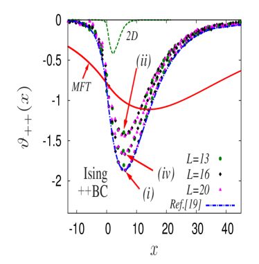
Figure 9: Scaling function $\vartheta_{++}$ of the critical Casimir force in the three-dimensional Ising model with $(++)$ BC and zero bulk field. Data points refer to lattices with fixed inverse aspect ratio $1/\rho=6$. The bottom and top data sets have been obtained by accounting for corrections to scaling according to Eq. (LABEL:eq:xy_f_fit1) (case (i)) and Eq. (LABEL:eq:xy_f_fit2) (case (ii)), respectively. The intermediate data set, instead, considers corrections of the rational form given by Eq. (LABEL:eq:fit_new) (case (iv)). In each case the data collapse turns out to be very good within the range of the scaling variable $x$ covered in the figure. The final estimate of the scaling function is biased by the functional form assumed for the corrections to scaling. The position $x_{\mathrm{min}}\simeq 5.90(8)$ of the minimum is insensitive with respect to these choices for the form of the corrections. For comparison we provide the prediction of mean-field theory krech (solid line), normalized such that $\vartheta_{++}^{\mathrm{(MFT)}}(0)=\vartheta_{++}^{\mathrm{(MC)}}(0)$ [Fig. 8(a)], the exact result for the two-dimensional Ising model ES (dashed line), and the result from the extended de Gennes-Fisher local-functional method bu-08 (dash-dotted line). Note that the actual phase transition of the film occurs at a nonzero value of the bulk field.

In the case of $(+-)$ BC we can compare $\vartheta_{+-}$ with the experimental results of Ref. pershan , with the prediction of mean-field theory krech and with the corresponding result for the two-dimensional Ising model ES (see Fig. 10). The solid line, normalized similarly as for $(++)$ BC, represents the MF result, whereas the dashed line refers to the two-dimensional Ising model ES . We expect the experimental data in Ref. pershan to be affected by corrections to scaling already for $x\gtrsim 2$, due to the relatively small corresponding value of $\xi/\ell\lesssim 30$, where $\ell\simeq 3$Å is the molecular scale set by the specific binary liquid mixture used in Ref. pershan . In view of these difficulties, the comparison between the MC and the experimental data in Fig. 10 can be regarded to provide an encouraging agreement.

Within the Derjaguin approximation our numerical results for $\vartheta_{++}$ and $\vartheta_{+-}$ form the basis for the calculation Hertlein of the corresponding scaling functions for the critical Casimir potentials in the sphere-plate geometry, which turn out to be in remarkably good agreement with the actual experimental results for that geometrical setting Hertlein .

Comparing the scaling functions for $d=2$, $3$, and $4$ (MFT) one finds that in the case of $(++)$ [$(+-)$] BC the position of the minimum [maximum] moves away from the bulk critical point $x=0$ as the spatial dimension increases. For $(++)$ [$(+-)$] BC the minimum [maximum] occurs above [below] $T_{c}$ for all $d$. The shapes of the scaling functions in $d=2$ and $d=3$ exhibit an interesting resemblance.

As we pointed out above, in the case of $(+-)$ BC the fluctuations of the order parameter are enhanced by the presence of a strongly fluctuating interface in the middle of the film. This results in a critical Casimir force which is generally stronger than in the case of $(++)$ BC, for which there is no such an interface. This is reflected by the fact that the amplitude $\vartheta_{+-}$ is larger than that of $|\vartheta_{++}|$, e.g., $\vartheta_{+-}^{\mathrm{(max)}}/|\vartheta_{++}^{\mathrm{(min)}}|\simeq 3.8$ for the data sets obtained by accounting for the corrections to scaling according to Eq. (LABEL:eq:xy_f_fit1) (case (i)) and Eq. (LABEL:eq:xy_f_fit2) (case (ii)). Even though field-theoretical MFT per se does not provide quantitative predictions for the overall amplitudes of the scaling functions $\vartheta_{++,+-}$, it yields the relation footnote2

$$\vartheta_{+-}^{\mathrm{(MFT)}}(x)=-4\vartheta_{++}^{\mathrm{(MFT)}}(-2x)$$ (27)

and therefore predicts $\vartheta_{+-}^{\mathrm{(max)}}/|\vartheta_{++}^{\mathrm{(min)}}|=4$ and that the maximum of $\vartheta_{+-}$ [minimum of $\vartheta_{++}$] occurs below [above] $T_{c}$. Thus MFT captures already quite well the qualitative and quantitative differences due to the presence or absence of an interface in the film. In addition, the fluctuations of such an interface, occurring in particular at low temperatures, cause the scaling function $\vartheta_{+-}$ to decay to zero for $x\rightarrow-\infty$ more slowly than the scaling function $\vartheta_{++}$, which is clearly visible by comparing Figs. 9 and 10.

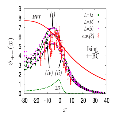
Figure 10: Scaling function $\vartheta_{+-}$ of the critical Casimir force in the three-dimensional Ising model with $(+-)$ BC and zero bulk field. Data points refer to lattices with fixed inverse aspect ratio $1/\rho=6$. For comparison we provide the mean-field prediction krech (solid line), normalized such that $\vartheta_{+-}^{\mathrm{(MFT)}}(0)=\vartheta_{+-}^{\mathrm{(MC)}}(0)$ [$=2\Delta_{+-}$, Fig. 8(b)], the exact result for the two-dimensional Ising model ES (dashed line), and the set of experimental data points from Ref. pershan . The top and bottom data sets have been obtained by accounting for corrections to scaling according to Eq. (LABEL:eq:xy_f_fit1) (case (i)) and Eq. (LABEL:eq:xy_f_fit2) (case (ii)), respectively. The intermediate data set, instead, considers corrections of the rational form given by Eq. (LABEL:eq:fit_new) (case (iv)). In each case the data collapse turns out to be very good for $x\geq-20$. The final estimate of the scaling function is biased by the functional form assumed for the corrections to scaling. The position $x_{\mathrm{max}}\simeq-5.4(1)$ of the maximum is insensitive with respect to these choices for the form of the corrections. In spite of this caveat the comparison with the experimental data is encouraging. Note that the actual phase transition of the film occurs at a nonzero value of the bulk field.

IV.2.2 Dirichlet-Dirichlet boundary conditions

In Fig. 11 we show the MC data corresponding to $g(y;L,2L,A)$ (see Eq. (12)) for the Ising model with $(O,O)$ BC, realized by free surface spins. The $L$-dependence of these data is quite pronounced and resembles that for the XY model with the same BC (compare Fig. 2(a)). On the other hand, the aspect ratio dependence appears to be relevant only in the narrow interval $-2\lesssim y\lesssim-1$ (see Fig. 12), which is similar to the case of the XY model with periodic BC (compare Fig. 3). As anticipated in Subsec. IV.1, the Ising model in a 3D film with Dirichlet-Dirichlet or periodic BC displays its 2D critical behavior at a critical point which is located on the bulk coexistence line $H=0$ at a size-dependent temperature $T_{c}(L)$ such that $T_{c}(L\rightarrow\infty)=T_{c}(1+y_{c}L^{-1/\nu})$ FSS , where $y_{c}$ is a non-universal constant which depends, inter alia, on the BC. From extrapolating the MC data for $T_{c}(L)$ reported in Table II of Ref. KOI-96 to $L\rightarrow\infty$ one infers $y_{c,OO}=-2.5(5)$ for the Ising model with $(O,O)$ BC. As in the case of the XY model, the residual dependence on $\rho$ observed in Fig. 12 might be due to the influence of the 2D phase transition for $y\simeq y_{c,OO}$. Such a dependence cannot be captured by ansätze such as the ones considered so far, which assume that the corrections to scaling due to $\rho\neq 0$ are independent of $x$. Therefore, in order to achieve a good collapse of the data sets corresponding to different lattice sizes we account for corrections to scaling by following the procedure applied to the XY model with $(O,O)$ BC, but we do not consider an aspect ratio dependence, i.e., we use the ansätze in Eqs. (18),  (LABEL:eq:xy_f_fit1) (case (i)), and  (LABEL:eq:xy_f_fit2) (case (ii)) with $r_{1,2}=0$. As a result of the fitting procedure in the interval $x\in[-7,-4]$ we find $g_{1}=6.55(8)$ and $g_{\omega}=2.35(3)$ in case (i), and $g_{2}=-2.877(15)$ and $g_{\omega}=2.35(3)$ in case (ii). Figure 13 shows the corresponding resulting estimates of the scaling function $\vartheta(x)$ of the critical Casimir force with an excellent data collapse. As before, we find that $\vartheta(x)$ is affected by the choice of the functional form of corrections to scaling. In the two cases (i) and (ii) one finds estimates of $\vartheta(x)$ which have the same shape but the overall amplitude is reduced by a factor $R\simeq 0.866$ in case (ii) compared with case (i).

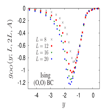
Figure 11: Monte Carlo data for $g_{OO}(y=\tau(L-\frac{1}{2})^{1/\nu};L,2L,A=(L/\rho)^{2})$ (see Eq. (12), $\tau=(T-T_{c})/T_{c}$) in the three-dimensional Ising model with $(O,O)$ BC for $L=8$, $12$, $16$, $20$, and for a fixed aspect ratio $\rho=1/6$. The 2D critical point of the film is located at $y=y_{c,OO}=-2.5(5)$, as inferred from extrapolating the data in Table II of Ref. KOI-96 to $L\rightarrow\infty$.

Due to the residual dependence on the aspect ratio $\rho$, $x_{\mathrm{min}}(\rho)$ and $\vartheta_{\mathrm{min}}(\rho)$ decrease upon decreasing $\rho$ and therefore the values of $\vartheta_{\mathrm{min}}$ and $x_{\mathrm{min}}$ quoted above overestimate the actual $\vartheta_{\mathrm{min}}(\rho=0)$ and $\vartheta_{\mathrm{min}}(\rho=0)$. The accuracy of our data does not allow us to study in more detail the Casimir amplitude $\Delta_{O,O}\equiv\vartheta(0)/2$ (as we did for $\Delta_{++}$ and $\Delta_{+-}$ in Fig. 8), which turns out to be very small for $(O,O)$ BC. Indeed the estimate from the partially resummed $\epsilon$-expansion is $\Delta_{O,O}=-0.0164$ krech , whereas MC simulations yield $\Delta_{O,O}=-0.0114(20)$ krech . However, from our data for the scaling function we can estimate $\Delta_{O,O}=-0.014(8)$. The corrections of form (i) yield for the pronounced minimum of the scaling function $x^{\mathrm{(i)}}_{\mathrm{min}}=-5.74(2)$ and $\vartheta^{\mathrm{(i)}}_{\mathrm{min}}\equiv\vartheta(x^{\mathrm{(i)}}_{\mathrm{min}})=-1.629(3)$ whereas those of form (ii) result in $x^{\mathrm{(ii)}}_{\mathrm{min}}=-5.73(4)$ and $\vartheta^{\mathrm{(ii)}}_{\mathrm{min}}\equiv\vartheta(x^{\mathrm{(ii)}}_{\mathrm{min}})=-1.41(1)$.

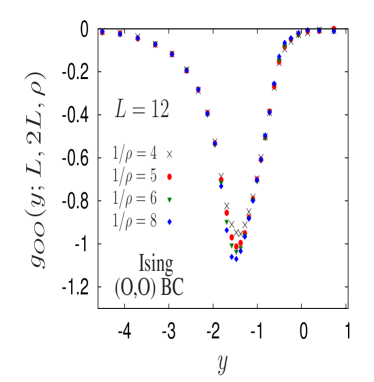
Figure 12: Monte Carlo data for $g_{OO}(y=\tau(L-\frac{1}{2})^{1/\nu};L,2L,A=(L/\rho)^{2})$ (see Eq. (12), $\tau=(T-T_{c})/T_{c}$) in the three-dimensional Ising model with $(O,O)$ BC for $L=12$ and various values of the inverse aspect ratio $1/\rho={\sqrt{A}}/L$.

In 2D the scaling functions obey the relation $\vartheta_{OO}(x)=\vartheta_{++}(-x)$ ES . We note that in 3D this relation holds approximately for the positions of the minima of the scaling functions ($x^{(O,O)}_{\mathrm{min}}\simeq-5.7,x^{(+,+)}_{\mathrm{min}}\simeq 5.90$) but for the $(O,O)$ BC the scaling function vanishes more rapidly than the scaling function for the $(++)$ BC. For comparison in Fig. 13 we provide the exact result for the two-dimensional Ising model (dashed line). In the inset we show our MC data corresponding to the case (i) together with the scaling function obtained by using the $\epsilon$-expansion in Ref. KD-92 . We note that it yields $\vartheta(0)/2=\Delta_{O,O}\simeq-0.0118$, which is larger than the estimate $\Delta_{O,O}\simeq-0.015$ given in the same paper KD-92 , and obtained from dimensional interpolation; the latter value is still larger than the more recent theoretical estimate $\Delta_{O,O}\simeq-0.0164$ in Ref. krech .

In the case of Dirichlet-Dirichlet boundary conditions discussed here, the film exhibits the 2D critical behavior at $T=T_{c}(L)$, corresponding to a universal value $x^{*}=y_{c}(\xi_{0}^{+})^{-1/\nu}$ of the scaling variable $x$. Close to the temperature $T_{c}(L)$, the free energy of the film is expected to exhibit the singularity $\sim|T-T_{c}(L)|^{2-\alpha_{\mathrm{2D}}}$, where $\alpha_{\mathrm{2D}}$ is the critical exponent of the specific heat of the two-dimensional system. This implies KD-92 that the scaling function $\vartheta_{OO}(x)$ of the Casimir force displays a singularity $\sim|x-x^{*}|^{2-\alpha_{\mathrm{2D}}}$ at $x=x^{*}$, i.e., $\sim(x-x^{*})^{2}\ln|x-x^{*}|$ for the Ising model. This singularity is too weak to be detectable by the present MC data. In Fig. 13 the gray bar indicates the value of $x^{*}_{OO}=y_{c,OO}(\xi_{0}^{+})^{-1/\nu}=-7.6(1.3)$ and the associated uncertainty. Accordingly, the singularity is expected to occur on the left side of the pronounced dip.

So far there are no experimental data available that would correspond to the Ising universality class with $(O,O)$ BC. For experiments with binary liquid mixtures the $(O,O)$ BC would correspond to walls which have no adsorption preferences, i.e., both components of the mixture are attracted equally by each surface. Effectively, in the limit of large film thicknesses, this can be achieved by chemically decorating the confining walls by stripes of equal width and alternating preferences for the two species of the binary liquid mixture (see Fig. 6 in Ref. sprenger for $S=1$, for which within MFT the effective Casimir amplitude vanishes, corresponding to vanishing surface fields within MFT so that $(O,O)$ BC hold).

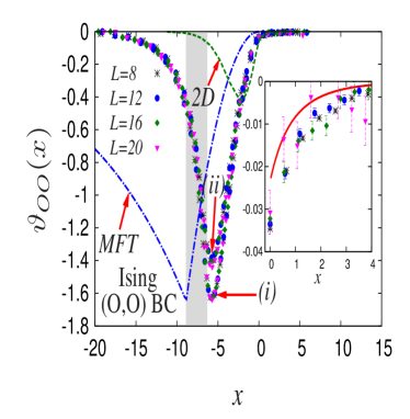
Figure 13: Scaling function $\vartheta_{OO}$ of the Casimir force for the three-dimensional Ising model with $(O,O)$ BC and zero bulk field. The MC data refer to lattices with $L=8$, $12$, $16$, $20$ and with a fixed inverse aspect ratio $1/\rho=6$. Corrections to scaling have been accounted for according to two different ansätze, provided by Eq. (LABEL:eq:xy_f_fit1) and Eq. (LABEL:eq:xy_f_fit2), and the corresponding numerical results are denoted by (i) and (ii), respectively. With corrections of the form (ii), the shape of the resulting scaling function is almost indistinguishable from the one obtained with corrections of the form (i), but its overall amplitude is reduced by a factor $R\simeq 0.866$. For comparison we show the exact result for the 2D Ising model ES (dashed line) and the mean-field prediction LGW-MF (dash-dotted line) normalized such that it yields the same depth of the minimum as the one of the MC data (i). In the inset we compare the MC data corresponding to the case (i) with the scaling function obtained from the $\epsilon$-expansion KD-92 . The gray bar indicates the value $x^{*}_{OO}=-7.6(1.3)$ (and its uncertainty) of the scaling variable $x$ corresponding to the occurrence of the shifted critical point, inferred from extrapolating the data in Table II of Ref. KOI-96 to $L\rightarrow\infty$.

IV.2.3 Periodic boundary conditions

In the case of periodic BC the aspect ratio dependence of the Monte Carlo data for the Ising model (as for the XY model discussed in Subsec. IV.1) turns out to be relevant only in the vicinity of the minimum of the function $g_{P}(y;L,2L,A)$ which is associated with the finite-size effects close to the actual critical point of the thin film. Extrapolating the data in Table I of Ref. KOI-96 to $L\rightarrow\infty$ one infers that the shifted critical point corresponds to $y=y_{c,P}=-1.60(2)$. The fact that this type of finite-size dependence does not occur for the Ising model with fixed BC (see Fig. 7) might be related to the different phase behavior below $T_{c}$ in the latter case. For $(++)$ BC the critical point is shifted off the bulk coexistence line $H=0$ to some value $(T_{c}(L),H_{c}(L))$ evans and hence in the vicinity of the minimum of the function $g_{++}(y;L,2L,A)$ the corresponding bulk correlation length is smaller than the characteristic transverse length $L_{\|}=\sqrt{A}$. As already mentioned earlier, for $(+-)$ BC below $T_{c}$ (but above the temperature of unbinding of this interface from one or the other surface) there exists a single film phase characterized by the OP profile displaying an interfacelike structure centered at the middle of the film parryevans ; binder . In this film phase the parallel correlation function $\xi_{\parallel}$ governing the exponential decay of correlations along the interface is very large even for temperatures further away from $T_{c}$, i.e., $\xi_{\parallel}\sim\exp(L_{\parallel}/(4\xi))$ with $L_{\parallel}=L_{x}=L_{y}$. $\xi_{\parallel}$ gives rise to the aspect ratio dependence of the function $g_{P}(y;L,2L,A)$ for $y\lesssim-4$.

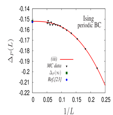
Figure 14: MC data for the critical Casimir amplitude $\Delta_{\mathrm{P}}(L)$ for the three-dimensional Ising model with periodic BC, as a function of the inverse film thickness $L$ (on lattices with fixed inverse aspect ratio $1/\rho=6$). Due to $L$-dependent corrections to scaling, $\Delta_{P}$ depends on $L$ and reaches its asymptotic value in the limit $L\rightarrow\infty$. The solid line corresponds to the best fit obtained by using the fitting ansatz given in Eq. (LABEL:eq:xy_f_fit3) in the interval $0<1/L\leq 0.25$. Our estimate ($\blacksquare$) for the asymptotic value of the Casimir amplitude $\Delta_{P}(\infty)$ compares very well with the previous MC result ($\bullet$) from Ref. krech .

In order to account for the corrections to scaling we follow the same procedure which we used for the XY model with periodic BC, i.e., we assume their $L$-dependence to be captured by Eq. (LABEL:eq:xy_f_fit3) at least within the range of sizes we are interested in. Accordingly, we focus on the data for the critical Casimir amplitude $\Delta_{P}$ and we fit them according to Eq. (24) (case (iii), Eq. (LABEL:eq:xy_f_fit3)). The best fit parameters, based on all data points, are given by $g_{3}=16.10(55)$ and $\omega_{{\rm eff}}=2.664(27)$ and the resulting curve is provided as a solid line in Fig. 14. The associated estimate for the asymptotic value $\Delta_{P}(L\to\infty)\equiv\Delta_{P}=-0.1520(2)$ agrees very well with the MC result $-0.1526(10)$ from Refs. krech ; KL .

The scaling function $\vartheta_{\mathrm{P}}$ can now be determined by assuming that Eq. (19), with $r_{2}=0$ and the parameters $g_{3}$ and $\omega_{{\rm eff}}$ obtained from the analysis of $\Delta_{P}(L)$, effectively describes its corrections to scaling (case (iii), Eq. (LABEL:eq:xy_f_fit3)), which actually leads to a very good data collapse in a wide range of temperatures. It also turns out that no corrections to the scaling variable $x$ (see Eq. (18)) are required in order to achieve it, i.e., $r_{1}$, $g_{\omega}\simeq 0$. (Note, however, that corrections due to $\rho\neq 0$ might be particularly relevant within a certain range of the scaling variable $x$, see below.) The resulting scaling function $\vartheta_{\mathrm{P}}$ is presented in Fig. 15 and it is based on a larger set of geometries of the simulation cell and with a better accuracy than in our earlier work EPL . The scaling function is in very good agreement with its previous determination in Ref. DK based on the computation of the lattice stress tensor. The slight discrepancies might be due to the uncertainty in the normalization factor which had to be used in Ref. DK (see also Subsec. IV.1). This agreement provides additional support concerning the reliability of our approach.

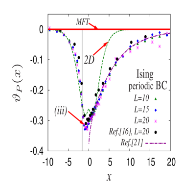
Figure 15: Scaling function $\vartheta_{\mathrm{P}}(x)$ of the critical Casimir force in the three-dimensional Ising model with periodic BC and zero bulk field. The data points refer to lattices with the inverse aspect ratio $1/\rho=6$. The corrections to scaling are taken into account according to Eqs. (19) and (LABEL:eq:xy_f_fit3) (case (iii)), see the main text). For comparison we show also the data set corresponding to the lattice with thickness $L=20$ as investigated in Ref. DK , the analytical prediction of Ref. GD (dash-dotted line) for $x\geq 0$, and results for 2D Ising model (dashed line) that we have obtained numerically by using the transfer matrix method. Due to the self-duality of the 2D Ising model one has $\vartheta_{\mathrm{P}}(-x)=\vartheta_{\mathrm{P}}(x)$ for $d=2$ which allows for the occurrence of two symmetric minima rudnick . We note that MFT yields $\vartheta_{\mathrm{P}}(x)\equiv 0$ (solid line). The gray vertical line indicates the universal value $x^{*}_{P}=-1.60(2)$ of the scaling variable $x$ corresponding to the occurrence of the shifted critical point, inferred from extrapolating the data in Table I of Ref. KOI-96 to $L\rightarrow\infty$.

Figure 15 presents also the comparison with the analytical prediction of the recently proposed field-theoretical (FT) expansion up to $O(\epsilon^{3/2})$ GD (dash-dotted line) for $x\geq 0$. This latter prediction is now in better agreement with the MC data than the previous $O(\epsilon)$ field-theoretical result in Ref. KD-92 but still misses the onset of the formation of the minimum. (Figure 5 in Ref. EPL compares the MC data with the $O(\epsilon)$ results, revealing a significant discrepancy for $0<x\lesssim 4$.) The estimated value of $\vartheta^{\mathrm{(FT)}}_{P}(0)=-0.39$ from Refs. DGS ; GD does not agree with our MC estimate $\vartheta_{P}(0)=-0.3040(4)$. For the minimum of the scaling function we find the estimates $x_{\mathrm{min}}=-0.681(1)$, $\vartheta_{\mathrm{min}}\equiv\vartheta_{\mathrm{P}}(x_{\mathrm{min}})=-0.329(1)$. Note, however, that for $x\simeq x_{\mathrm{min}}$ the corrections due to $\rho\neq 0$ are expected to be relevant. In order to substantiate this statement we have determined the function $g_{\mathrm{P}}(y;L,2L,A=(L/\rho)^{2})$ (see Eq. (12)) also from a set of data for lattices of thickness $L=10$ and $15$ with an inverse aspect ratio $\rho^{-1}=14$, which can be compared with the corresponding data set from Fig. 15, for which $\rho^{-1}=6$. This comparison is presented in Fig. 16 and clearly shows that, while the function $g_{\mathrm{P}}$ is actually only slightly dependent on the thickness $L$ of the lattice, there is a dependence on $\rho$ which, however, is relevant only very close to $x_{\mathrm{min}}$. As mentioned above for the case of $(O,O)$ BC, this latter dependence on $\rho$ cannot be captured by ansätze such as the ones considered so far because they assume $x$-independent corrections due to $\rho\neq 0$. Therefore, similar to the case of $(O,O)$ BC, due to the residual dependence on $\rho$, $x_{\mathrm{min}}(\rho)$ and $\vartheta_{\mathrm{min}}(\rho)$ decrease upon decreasing $\rho$ and therefore the values of $\vartheta_{\mathrm{min}}$ and $x_{\mathrm{min}}$ quoted above overestimate the actual values of $\vartheta_{\mathrm{min}}(\rho=0)$ and $x_{\mathrm{min}}$.

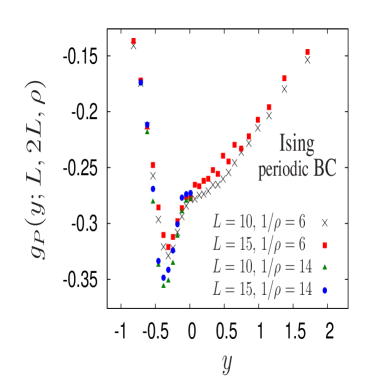
Figure 16: Aspect-ratio dependence of the function $g_{\mathrm{P}}(y=\tau(L-\frac{1}{2})^{1/\nu};L,2L,A=(L/\rho)^{2})$ (see Eq. (12)) for the three-dimensional Ising model with periodic BC. For a fixed value of $\rho$, this function depends only weakly on $L$. By changing $\rho$, the function $g_{\mathrm{P}}$ is affected mainly in the region $-0.6\lesssim y\lesssim 0$. The 2D critical point of the film is located at $y=y_{c,P}=-0.52(2)$, as inferred from extrapolating the data in Table I of Ref. KOI-96 to $L\rightarrow\infty$.

As in the case of Dirichlet-Dirichlet boundary conditions, the point at which the film exhibits the 2D critical behavior is located on the bulk coexistence line and corresponds to a value $x^{*}$ of the scaling variable $x$, at which the scaling function is expected to display the weak singularity $\sim(x-x^{*})^{2}\ln|x-x^{*}|$ (see Sec. IV.2.2 above). In Fig. 15 the gray vertical line indicates the corresponding universal value $x^{*}_{P}=y_{c,P}(\xi_{0}^{+})^{-1/\nu}=-1.60(2)$. Accordingly, also in this case the singularity is expected to occur on the left side of the pronounced dip but cannot be detected by the present MC data.

As a final remark we point out that for the Ising model with periodic BC the function $g_{P}(y;L,2L,A)$ exhibits a somewhat peculiar shape near $T_{c}$ with a characteristic “shoulder” formed above the critical temperature. The procedure for retrieving the scaling function $\hat{\theta}(y)$ [the lattice estimate of $\theta(y)\equiv\vartheta_{\mathrm{P}}(y/(\xi_{0}^{+})^{1/\nu})$] via Eq. (13) involves rescaling of the argument of the scaling function and removes the “shoulder” structure from the curve. The formation of this “shoulder” is related to the particular shape of $\vartheta_{\mathrm{P}}$ which on the left side of the minimum increases more steeply than on the right side of it (see Fig. 17).

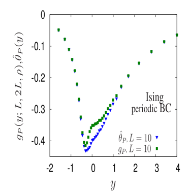
Figure 17: Plot of the function $g_{\mathrm{P}}(y;L,2L,A=(L/\rho)^{2})$ (see Eq. (12)) and the associated scaling function $\hat{\theta}(y)$ (i.e., the lattice estimate of $\theta(y)\equiv\vartheta_{\mathrm{P}}(y/(\xi_{0}^{+})^{1/\nu})$, which is calculated by solving Eq. (12)) iteratively for the three-dimensional Ising model with periodic BC. The data points refer to a lattice with $L=10$ and $1/\rho=6$. The data have not been corrected for the corrections to scaling. The pronounced shoulder originally present in $g_{P}$ is smoothed out upon calculating the associated scaling function.

V Summary and conclusions

A. Summary

We have presented important details of a novel general approach EPL to determine the universal scaling functions $\vartheta$ of critical Casimir forces via MC simulations. We have applied this method (see Subsects. III.1 and III.2 as well as Fig. 1) in order to study the scaling functions corresponding to the three-dimensional Ising and XY bulk universality classes for a variety of universal boundary conditions in film geometries with varying thickness $L$. Corrections to scaling appear to be quite relevant in the range of sizes $L$ we have investigated, which are strongly limited by the steeply increasing computational costs required for larger systems. In spite of these difficulties, it is possible to analyze the corresponding MC data by assuming suitable ansätze for corrections to scaling. Even if the final numerical determinations of the scaling functions are biased by these assumptions, they turn out to be consistent with the results of different numerical and analytical approaches and with all available experimental data.

Our main results are the following:

(1) We have obtained the Casimir scaling function $\vartheta_{OO}$ for the three-dimensional XY model with $(O,O)$ BC [(Dirichlet, Dirichlet) BC] (Fig. 4). Corrections to scaling have been accounted for by using two different ansätze, provided by Eq. (LABEL:eq:xy_f_fit1) (case (i)) and Eq. (LABEL:eq:xy_f_fit2) (case (ii)). These choices of the functional form of corrections to scaling have been dictated by the pronounced dependences on $L$ and on the aspect ratio $\rho$ of the simulation cell which occur for this type of BC (Fig. 2(a)). Both ansätze lead to a very good data collapse but the overall amplitude of the scaling function is reduced by a factor $R\simeq 0.9$ in case (ii) compared to case (i). Our MC data compare very well with the corresponding experimental data for ⁴He films from Ref. garcia and with the MC data of Ref. hucht . For comparison also mean field results are provided.

(2) The Casimir scaling function $\vartheta_{P}$ and the critical Casimir amplitude $\Delta_{P}$ have been obtained for the three-dimensional XY model with periodic BC (Figs. 6 and 5). In this case, judged by the behavior of the generating function $g$ introduced in Eq. (12), corrections to scaling are much less pronounced than in the case of $(O,O)$ BC (Fig. 2(b)) and the aspect ratio dependence is relevant only in the restricted range of the scaling variable near the minimum of the scaling function (Fig. 3). A very good data collapse is achieved by using the ansatz with the effective exponent $\omega_{{\rm eff}}=2.59(4)$ (Eq. (LABEL:eq:xy_f_fit3) (case (iii)) and by neglecting the corrections to scaling due to the aspect ratio dependence ($r_{1,2}=0$ in Eqs. (18) and (19)). The shape of our MC data agree very well with the corresponding MC data of Ref. DK which, however, have left the amplitude undetermined. Our estimate for the critical Casimir amplitude is $\Delta_{P}=-0.2993(7)$. By extending the line of arguments of Ref. kardar:04 to the present case, we have theoretically predicted the value $\vartheta_{P}^{\rm(TH)}(-\infty)=-\zeta(3)/\pi\simeq-0.38$ [see Eq. (25)] at which the scaling function $\vartheta_{P}(x)$ saturates for $x\rightarrow-\infty$. This value is confirmed by the corresponding estimate $-0.383(4)$ based on our MC data.

(3) We have obtained the scaling functions $\vartheta_{++}$, $\vartheta_{+-}$ and the corresponding Casimir amplitudes $\Delta_{++},\Delta_{+-}$ of the critical Casimir force in the three-dimensional Ising model with $(++)$ and $(+-)$ BC, respectively, applicable for classical fluids (Figs. 9, 10 and 8). We find that in the critical regime the numerical data are practically independent of the aspect ratio $\rho$ (Fig. 7) but $L$-dependent corrections to scaling are rather important (Fig. 8). The presented scaling functions and Casimir amplitudes have been obtained by accounting for corrections to scaling according to Eq. (LABEL:eq:xy_f_fit1) (case (i)), Eq. (LABEL:eq:xy_f_fit2) (case (ii)), and Eq. (LABEL:eq:fit_new) (case (iv)) with $r_{1,2}=0$ (thus neglecting the dependence of the data on $\rho$). The final estimate of the scaling function is biased by the functional form assumed for the corrections to scaling; all considered cases provide a very good data collapse. The fitting ansatz in Eq. (26) describes very well the data for the Casimir amplitudes $\Delta_{++/+-}$ as a function of the film thickness $L$. Our estimates for the asymptotic values of the Casimir amplitudes are $\Delta_{++}=-0.376(29)$ and $\Delta_{+-}=2.71(2)$ which compare reasonably well with previous MC results from Ref. krech and with the results from the de Gennes-Fisher local-functional approach upton . Our results for the case of $(+-)$ BC compare well with recent X-ray scattering data for critical films of a classical binary liquid mixture pershan . Moreover the MC data for the scaling functions $\vartheta_{++}$ and $\vartheta_{+-}$ have been used to calculate, within the Derjaguin approximation, the corresponding scaling functions for the critical Casimir potentials for the experimentally relevant geometry of a sphere near a planar substrate. These numerical results agree remarkably well with the experimental data for colloidal particles immersed in a critical solvent and close to a container wall Hertlein .

(4) We have obtained the Casimir scaling function $\vartheta_{OO}$ for the three-dimensional Ising model with $(O,O)$ BC (Fig. 13). For these BC the $L$-dependence of the MC simulation data is quite pronounced (Fig. 11), similarly to the case of the XY model with the same $(O,O)$ BC. The dependence on the aspect ratio is relevant only in the small range of the scaling variable near the minimum of the scaling function (Fig. 12). Our data do not allow us to obtain a quantitatively accurate estimate of the Casimir amplitude, because of its very small value. Corrections to scaling have been accounted for according to the ansätze provided by Eq. (LABEL:eq:xy_f_fit1) (case (i)) and Eq. (LABEL:eq:xy_f_fit2) (case (ii)) with $r_{1,2}=0$ (thus neglecting the dependence of the data on the aspect ratio $\rho$).

(5) The scaling function $\vartheta_{\mathrm{P}}(x)$ and the critical Casimir amplitude $\Delta_{\mathrm{P}}$ have been obtained for the three-dimensional Ising model with periodic BC (Figs. 15 and 14). As in the case of the XY model with periodic BC, the aspect ratio dependence of the MC data appears to be pronounced only near the actual critical point of the thin film (Fig. 16). Therefore, the corrections to scaling have been accounted for in the same way as for the XY model with periodic BC, i.e., according to Eqs. (19) and (LABEL:eq:xy_f_fit3) (case (iii)). The best fit for the $L$-dependence of the Casimir amplitude $\Delta_{\mathrm{P}}$ has been obtained by using the ansatz given in Eq. (26). Our improved estimate for the value of the Casimir amplitude $\Delta_{P}=-0.1520(2)$ agrees very well with the previous MC result from Refs. krech ; KL . The particular shape of the scaling function $\vartheta_{\mathrm{P}}(x)$ around its minimum is reflected in the formation of a characteristic “shoulder” in the corresponding generating function $g_{P}$ above the critical temperature (Fig. 17).

B. Conclusions and outlook

Our approach can be applied in order to study other experimentally relevant geometrical settings as well as the effect of chemically or geometrically inhomogeneous confining surfaces on the critical Casimir force. In the latter cases, even lateral critical Casimir forces are expected to act in addition to the normal Casimir force investigated here. This lateral force has been theoretically investigated for chemically SSD-06 and topographically THD-08 patterned surfaces, whereas it has been experimentally studied for colloidal particles exposed to chemically patterned surfaces CPS .

In addition to appliying our quantitative method to these cases, it is also desirable to perform more extensive and larger scale MC simulations in order to identify the origins of the corrections to scaling and to characterize them more accurately, possibly to the extent which is by now achieved for bulk critical phenomena. This valuable knowledge would therefore allow an unbiased and thus even more accurate determination of the scaling functions of the critical Casimir force beyond the results presented here. Finally, beyond the application to thin ⁴He films near the superfluid-normal fluid transition, our results for the three-dimensional XY model with $(O,O)$ BC could be relevant for critical Casimir forces acting on Bose-Einstein condensates martin .

Appendix A Corrections to scaling and fitting procedures.

In this appendix we describe the general strategy we have used in order to obtain the best fitted values of the parameters which control the corrections to scaling. The main problems one faces are to quantify the quality of a certain data collapse and then to choose the parameters which influence it in such a way as to optimize this quality. The estimation of the parameters and of the associated confidence interval proceeds as in the case of least-square fits with chi-square tests of the quality of the fit, but with the additional complication that the fitting function itself is not known and has to be estimated from the numerical data itself.

In what follows we describe the procedure we have used in order to determine the best fit parameters which control the $L$-dependent corrections to scaling. On the same footing we have also treated the corrections due to a nonzero aspect ratio $\rho\neq 0$ (see Subsec. III.4). In full generality, assume that one seeks to determine, e.g., via MC simulations, the finite-size scaling function $h$ of a quantity $\psi$ which, in the absence of corrections to scaling, is expected to be a function of a scaling variable $x$ only (which involves a suitable combination of temperature and size $L$ of the system) so that

$$\psi(x,L\to\infty)=h(x).$$ (28)

For the time being we omit possible algebraic $L$-dependent prefactors of $h$. In the MC simulations one considers a set of $N$ lattices of sizes $L_{1}$, $L_{2}$, …, $L_{N}$ and by varying the temperature one collects for each size $L_{k}$ a discrete set of numerical values $\psi_{k,j}$ of $\psi$ with $j=1,2\ldots,j_{k}^{\mathrm{max}}$ which correspond to values $x_{k,j}$ of the scaling variable $x$ in the interval $[x_{\mathrm{min}},x_{\mathrm{max}}]$. In this process the statistical uncertainty $\Delta\psi_{k,j}$ associated with $\psi_{k,j}$ is also determined. From these quantities $\psi_{k,j}$ one intends to determine $h$, taking into account the presence of corrections to scaling. Due to them, $\psi$ is actually not a function of $x$ only, but also of the size $L$ of the system. In order to cope with this one therefore assumes the following functional structure:

$$\psi(x;L)=f_{1}(L;t_{1})h(f_{2}(L;t_{2})x)$$ (29)

where $f_{1}(L;t_{1})$ and $f_{2}(L;t_{2})$ capture the effects of the correction to scaling on the quantity $\psi$ itself and on the scaling variable $x$, respectively. These functions depend on the size $L$ of the system and on certain parameters $t_{1},t_{2}$ which one would like to determine in such a way as to achieve the best data collapse for the function $h$, obtained from the set of data points $(f_{2}(L_{k};t_{2})x_{k,j},[f_{1}(L_{k},t_{1})]^{-1}\psi_{k,j})=:(y_{k,j}(t_{1},t_{2}),h_{k,j}(t_{1},t_{2}))$ for the various values of $j$ and $k$, and as to take also into account the statistical error $\Delta h_{k,j}(t_{1}):=[f_{1}(L_{k},t_{1})]^{-1}\Delta\psi_{k,j}$ associated with $h_{k,j}(t_{1},t_{2})$.

For each value $L_{k}$ we have interpolated the data set $(x_{k,j},\psi_{k,j})$ in the interval $[x_{\mathrm{min}},x_{\mathrm{max}}]$ by using a cubic spline approximation. This way we have constructed a function $\psi_{k}(x)$ with $x\in[x_{\mathrm{min}},x_{\mathrm{max}}]$ and with $\psi_{k}(x_{k,j})=\psi_{k,j}$. From this function we have calculated the corresponding $L_{k}$-dependent estimate $h_{k}(x;t_{1},t_{2})$ of $h$, given by

$$h_{k}(y;t_{1},t_{2})=f_{1}(L_{k};t_{1})^{-1}\psi_{k}(yf_{2}(L_{k};t_{2})^{-1}),$$ (30)

which fulfills $h_{k}(y_{k,j}(t_{1},t_{2});t_{1},t_{2})=h_{k,j}(t_{1},t_{2})$. In order to assess the quality of the data collapse and the quality of the fit we have actually to specify the function with which we would like to fit the data, which is the yet unknown scaling function $h$. In order to achieve this, we define an expected model function $h_{\mathrm{expect}}$ as the average of the various $h_{k}$,

$$h_{\mathrm{expect}}(y;t_{1},t_{2})=\frac{1}{N}\sum\limits_{k=1}^{N}h_{k}(y;t_{1},t_{2}),$$ (31)

which will then be fitted to the observed MC values by adjusting the parameters $t_{1}$ and $t_{2}$.

Accordingly, we calculate the “$\chi^{2}(t_{1},t_{2})$” associated with the fitting of the data points $(y_{k,j}(t_{1},t_{2}),h_{k,j}(t_{1},t_{2}))$ with the function $h_{\mathrm{expect}}(y;t_{1},t_{2})$:

$$\begin{split}&\chi^{2}(t_{1},t_{2})=\\ &\sum\limits_{k=1}^{N}\sum\limits_{j=1}^{j_{k}^{\mathrm{max}}}\frac{[h_{k,j}(t_{1},t_{2})-h_{\mathrm{expect}}(y_{k,j}(t_{1},t_{2});t_{1},t_{2})]^{2}}{[\Delta h_{k,j}(t_{1})]^{2}}.\end{split}$$ (32)

Due to the non-trivial and non-linear dependence of the fitted data (and of the fitting function) on the parameters $t_{i}$ we cannot assume this quantity to play the same role as a $\chi^{2}$ in more standard fitting procedures in which only the fitting function depends on the parameters one wants to estimate. Nevertheless, we have heuristically made this assumption, i.e., that $\chi^{2}(t_{1},t_{2})$ plays the same role as a $\chi^{2}$, in order to determine the best fit parameters and the associated confidence intervals. Accordingly we have proceeded as usual by determining the optimal fit parameters $\bar{t}_{1}$ and $\bar{t}_{2}$ which minimize the value of $\chi^{2}$: $\chi^{2}(\bar{t}_{1},\bar{t}_{2})=\min_{\{t_{1},t_{2}\}}\chi^{2}(t_{1},t_{2})$. In order to estimate the statistical uncertainty $\Delta\bar{t}_{i}$ of $\bar{t}_{i}$ we have determined that region of the plane $(t_{1},t_{2})$ for which $\chi^{2}(t_{1},t_{2})<\chi^{2}(\bar{t}_{1},\bar{t}_{2})+2.3$ Bev . The projection of the resulting region (typically of the form of an ellipse) onto the axis $t_{i}$ gives $2\Delta\bar{t}_{i}$, so that the estimate for the parameters is of the form $\bar{t}_{i}\pm\Delta\bar{t}_{i}$.

References

- (1) M. E. Fisher and P. G. de Gennes, C. R. Acad. Sci. Paris Ser. B 287, 207 (1978).
- (2) M. N. Barber in Phase Transitions and Critical Phenomena, edited by C. Domb and J. L. Lebowitz (Academic, New York, 1983), Vol. 8, p. 149; V. Privman, in Finite Size Scaling and Numerical Simulation of Statistical Systems, edited by V. Privman (World Scientific, Singapore, 1990), p. 1.
- (3) Earlier observations bey of flocculation in colloidal suspensions close to the critical demixing point of a binary liquid mixture suggested the action of critical Casimir forces; however, an unquestionable conclusion could not be reached.
- (4) D. Beysens and D. Estève, Phys. Rev. Lett. 54, 2123 (1985); D. Beysens and T. Narayanan, J. Stat. Phys. 95, 997 (1999).
- (5) R. Garcia and M. H. W. Chan, Phys. Rev. Lett. 83, 1187 (1999); A. Ganshin, S. Scheidemantel, R. Garcia, and M. H. W. Chan, Phys. Rev. Lett. 97, 075301 (2006).
- (6) M. Krech and S. Dietrich, Phys. Rev. Lett. 66, 345 (1991); Phys. Rev. A 46, 1886 (1992); Phys. Rev. A 46, 1922 (1992).
- (7) M. Krech and S. Dietrich, Phys. Rev. A 46, 1886 (1992).
- (8) M. Fukuto, Y. F. Yano and P. S. Pershan, Phys. Rev. Lett. 94, 135702 (2005).
- (9) S. Rafaï, D. Bonn, and J. Meunier, Physica A 386, 31 (2007).
- (10) R. Garcia and M. H. W. Chan, Phys. Rev. Lett. 88, 086101 (2002).
- (11) C. Hertlein, L. Helden, A. Gambassi, S. Dietrich, and C. Bechinger, Nature 451, 172 (2008).
- (12) O. Vasilyev, A. Gambassi, A. Maciołek, and S. Dietrich, EPL 80, 60009 (2007).
- (13) M. Krech, Casimir Effect in Critical Systems (World Scientific, Singapore, 1994); J. Phys.: Condens. Matter 11, R391 (1999).
- (14) J. G. Brankov, D. M. Dantchev, and N. S. Tonchev, The Theory of Critical Phenomena in Finite-Size Systems - Scaling and Quantum Effects (World Scientific, Singapore, 2000).
- (15) H. W. Diehl, in Phase Transitions and Critical Phenomena, edited by C. Domb and J. L. Lebowitz (Academic, London, 1986), Vol. 10, p. 76.
- (16) D. Dantchev and M. Krech, Phys. Rev. E 69, 046119 (2004).
- (17) A. Hucht, Phys. Rev. Lett. 99, 185301 (2007).
- (18) Z. Borjan and P. J. Upton, Phys. Rev. Lett. 81, 4911 (1998), and references therein.
- (19) Z. Borjan and P. J. Upton, Phys. Rev. Lett. 101, 125702 (2008).
- (20) H. W. Diehl, D. Grüneberg, and M. A. Shpot, Europhys. Lett. 75, 241 (2006).
- (21) D. Grüneberg and H. W. Diehl, Phys. Rev. B 77, 115409 (2008).
- (22) R. Evans and J. Stecki, Phys. Rev. B 49, 8842 (1994).
- (23) M. Krech, Phys. Rev. E 56, 1642 (1997).
- (24) C. Ruge, P. Zhu, and F. Wagner, Physica A 209, 431 (1994).
- (25) A. P. Gottlob and M. Hasenbusch, Physica A 201, 593 (1993).
- (26) A. Pelissetto and E. Vicari, Phys. Rep. 368, 549 (2002).
- (27) F. M. Schmidt and H. W. Diehl, Phys. Rev. Lett. 101, 100601 (2008).
- (28) R. Zandi, J. Rudnick, and M. Kardar, Phys. Rev. Lett. 93, 155302 (2004). The correct numerical value of the scaling function of the force at very low temperatures, following from the analytic expression in Eq.(11) therein, is instead of the indicated . As also pointed out in Ref. hucht , this results in a larger difference between theory and the experimental data, as compared to the one presented therein.
- (29) A. Maciołek, A. Gambassi, and S. Dietrich, Phys. Rev. E 76, 031124 (2007).
- (30) R. Zandi, A. Shackell, J. Rudnick, M. Kardar, and L. P. Chayes, Phys. Rev. E 76, 030601(R) (2007).
- (31) K. K. Mon, Phys. Rev. B 39, 467 (1989); K. K. Mon and K. Binder, Phys. Rev. B 42, 675 (1990).
- (32) D. P. Landau and K. Binder, A Guide to Monte Carlo Simulations in Statistical Physics (Cambridge University Press, London, 2005), p. 155.
- (33) V. Privman and M. E. Fisher, J. Phys. A 16, L295 (1983).
- (34) J. M. Luck, Phys. Rev. B 31, 3069 (1985).
- (35) K. K. Mon and M. P. Nightingale, Phys. Rev. B 35, 3560 (1987).
- (36) D. Dantchev, F. Schlesener, and S. Dietrich, Phys. Rev. E 76, 011121 (2007).
- (37) J. M. Kosterlitz and D. J. Thouless, J. Phys. C 6, 1181 (1973).
- (38) W. Janke and K. Nather, Phys. Rev. B 48, 15807 (1993).
- (39) A. Schmidt and T. Schneider, Z. Phys. B 87, 265 (1992).
- (40) M. Hasenbusch, arXiv:0811.2178 (2008).
- (41) N. Schultka and E. Manousakis, Phys. Rev. B 51, 11712 (1995).
- (42) F. M. Gasparini, M. O. Kimball, K. P. Mooney, and M. Diaz-Avila, Rev. Mod. Phys. 80, 1009 (2008).
- (43) W. Y. Tam and G. Ahlers, Phys. Rev. B 32, 5932 (1985).
- (44) The experimental value 1.2 Å used in Ref. LGW-MF1 is not the correct one for the comparison presented therein. The correct comparison of the experimental data with the mean-field analytical prediction LGW-MF ; LGW-MF1 and with the results of Monte Carlo simulations is presented here and in Refs. LGW-MF ; EPL ; hucht .
- (45) D. Dantchev, M. Krech, and S. Dietrich, Phys. Rev. Lett. 95, 259701 (2005).
- (46) A. O. Parry and R. Evans, Phys. Rev. Lett. 64, 439 (1990).
- (47) This relation between and has seemingly been overlooked in the literature even though it follows after some algebra from the analytic expressions of the scaling functions reported in Ref. krech . In particular it also follows that has a minimum for , whereas has a maximum for (which improves the estimates reported in the caption of Fig. 1 in Ref. krech ).
- (48) H. Kitatani, M. Ohta, and N. Ito, J. Phys. Soc. Jpn. 65, 4050 (1996).
- (49) M. Sprenger, F. Schlesener, and S. Dietrich, J. Chem. Phys. 124, 134703 (2006).
- (50) R. Evans, J. Phys. Condens. Matter 2, 8989 (1990).
- (51) K. Binder, Annu. Rev. Mater. Res. 38, 123 (2008).
- (52) M. Krech and D. P. Landau, Phys. Rev. E 53, 4414 (1996).
- (53) An independently derived analytic result for the Casimir scaling function of the 2D Ising model with periodic boundary conditions has been recently presented by J. Rudnick during the KITP program on the theory and practice of fluctuation-induced interactions at the University of California, Santa Barbara, http://online.itp.ucsb.edu/online/fluctuate08/rudnick/.
- (54) M. Sprenger, F. Schlesener, and S. Dietrich, J. Chem. Phys. 124, 134703 (2006).
- (55) M. Tröndle, L. Harnau, and S. Dietrich, J. Chem. Phys. 129, 124716 (2008).
- (56) F. Soyka, O. Zvyagolskaya, C. Hertlein, L. Helden, and C. Bechinger, Phys. Rev. Lett. 101, 208301 (2008).
- (57) P. A. Martin and V. A. Zagrebnov, Europhys. Lett. 73, 15 (2006); A. Gambassi and S. Dietrich, Europhys. Lett. 74, 754 (2006).
- (58) P. R. Bevington, Data Reduction and Error Analysis for the Physical Sciences (McGraw-Hill, New York, 1969).