Frequency dependent deformation of liquid crystal droplets in an external electric field

Abstract

Nematic droplets suspended in the isotropic phase of the same substance were subjected to alternating electrical fields of varying frequency. To keep the system at a constant nematic/isotropic volume ratio with constant droplet size we carefully kept the temperature in the isotropic/nematic coexistence region, which was broadened by adding small amounts of a non-mesogenic liquid. Whereas the nematic droplets remained spherical at low (in the order of 10 Hz) and high frequencies (in the order of 1 kHz), at intermediate frequencies we observed a marked flattening of the droplets in the plane perpendicular to the applied field. Droplet deformation occurred both in liquid crystals (LCs) with positive and negative dielectric anisotropy. The experimental data can be quantitatively modelled with a combination of the leaky dielectric model and screening of the applied electric field due to finite conductivity.

I Introduction

Liquid crystal droplets dispersed in isotropic media have attracted strong interest. Driven by new applications, during the last few years the research focus has shifted from studying the director field and defect structure in quasi-static situations (see, e.g., Crawford and Zumer (1996) (Eds.); Candau et al. (1973); Doane et al. (1986); Chan (1999); Lubensky et al. (1998); Dolganov et al. (2007)) to dynamic processes under the influence of external fields Park et al. (1994); Lev et al. (2001); Wu et al. (2007); El-Sadek et al. (2007). Due to the anisotropic nature of the liquid crystalline phases, these droplets show a much richer physics than purely isotropic systems.

The literature on the behavior of liquid crystalline droplets subjected to external fields is dominated by studies on droplets suspended in a non-mesogenic carrier fluid. Owing to the increasing importance of polymer dispersed liquid crystals in various applications, the scientific interest in the response of droplets to external field has grown significantly (for reviews see, e.g., Crawford and Zumer (1996) (Eds.); Coates (1995); Bouteiller and LeBarny (1996); Bunning et al. (2000); Tjong (2003); Jeon et al. (2007)). In addition, magnetic Candau et al. (1973) and shear fields Wu et al. (2007) have been applied to these systems. Only few studies have been carried out on liquid crystals in the coexistence region. Park and coworkers Park et al. (1994) studied nematic droplets in a quasi 2-dimensional system submitted to an electric field superimposed with a temperature gradient. Dolganov and coworkers Dolganov et al. (2007) investigated nematic droplets confined by a surrounding smectic phase.

Inevitable impurities in liquid crystal samples are known to open up a coexistence region between the nematic and isotropic phase (see, e.g., Chiu and Kyu (1995); Shen and Kyu (1995); Lin et al. (1998); DasGupta et al. (2001); Mukherjee (2002)). This coexistence region allows to have nematic droplets immersed in the isotropic phase of the same liquid at constant sample temperature. The physics of droplets in the isotropic-nematic coexistence region is peculiar because, unlike typical liquid-liquid interfaces, the interfacial tension is very low. Since droplet deformation always implies an increase in surface area, the higher the surface tension, the more rigid the droplets appear. In contrast, droplets in the nematic-isotropic coexistence region have a surface tension Langevin and Bouchiat (1973); Faetti and Palleschi (1984); Williams (1976); Yokoyama et al. (1985) of the order of $10^{-5}$ Nm and can be deformed very easily.

In this paper, we discuss electric field-induced droplet deformations that are peculiar to systems with low interfacial tension. We put special emphasis on the influence of field frequency, and the actual electric field strength. Moreover, we took special care to avoid electrochemical reactions in the sample that might influence the results. The paper is organized as follows: In Sec. II we describe the materials and the experimental set-up. In Sec. III.1, we present the results on the droplet deformation in the colloid-free systems. Sec. III.2 is devoted to investigating the underlying hydrodynamic flow field by adding tracer colloids to the system. We then compare our results to theoretical predictions in Sec. IV.

II Experimental details

Both the electric and dielectric properties of nematic liquid crystals are markedly anisotropic. Whereas the conductivity $\sigma$ typically exhibits positive anisotropy

$$\sigma_{\parallel}>\sigma_{\perp}$$ (1)

(the indices $\parallel$ and $\perp$ indicating the conductivity parallel and perpendicular to the nematic director $\hat{n}$, respectively), the anisotropy of the dielectric constant $\epsilon$ can vary (and change sign) between different substances

$$\epsilon_{\parallel}\lessgtr\epsilon_{\perp}.$$ (2)

We chose a typical representative for either class: methyloxybenzylidenbutylaniline (MBBA, Frinton Laboratories, USA, $\Delta\epsilon<0$) and pentylcyanobiphenyl (5CB, Chemos, Germany, $\Delta\epsilon>0$). Both chemicals were used as supplied. Impurities like polymers or low molecular weight organic sovents in liquid crystals lead to coexistence of the nematic and the isotropic phase within a certain temperature interval Shen and Kyu (1995); Lin et al. (1998); Roussel et al. (2000); Ullrich et al. (2006) (see Fig.1 for a schematic representation of the phase diagram). In our experiments, adding octane (Aldrich, analytic grade) at a concentration of $c_{e}=2$ vol% resulted in a coexistence interval of the order of 1.5 K, which is sufficient to override the effect of any impurities inevitably present in commercially available liquid crystals. The results presented in this paper did not change for octane concentrations between 1 and 4 vol%.

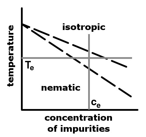
Figure 1: Schematic phase diagram of a liquid crystal with added impurities (in this work: octane). With increasing octane concentration, the nematic isotropic phase transition shifts to lower temperatures and a nematic-isotropic coexistence region opens. The temperature $T_{e}$ and the octane concentration $c_{e}$ (gray lines) were chosen be well within the coexistence region.

Poly(methyl methacrylate) particles (PMMA) with a radius of approximately 500 nm sterically stabilized by chemically grafted poly(12-hydroxy-stearic acid) molecules Antl et al. (1986); Bosma et al. (2002) were used as tracer particles.

As depicted in Fig. 2, the sample was placed between two glass slides of $\approx 170$ $\mu$m each. The outer side of these slides was covered with transparent indium-tin-oxide (ITO) electrodes. This configuration ensured that there was no electric contact between the electrodes and the sample. The surface of the glass slides was otherwise untreated. The sample cell was temperature controlled to a precision better than 0.05 K using a Linkam heating stage (THMS 600). All observations were performed using an Olympus BX51 optical microscope with a long working distance 20x objective and equipped with a CCD camera. For better contrast and good resolution of droplet edges, the sample was placed between parallel polarizers. The ITO electrodes allowed to subject the sample to an alternating electric field parallel to the light path of up to 0.4 V/$\mu$m and with frequencies up to 5 kHz. An oscilloscope was used to ensure that the applied voltage remained constant over the whole frequency range.

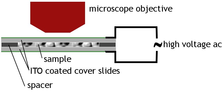
Figure 2: The sample was placed between two ITO coated glass slides (purchased form SPI Supplies) without direct contact between the sample and the electrodes. The sample thickness is approximately 180 $\mu$m and the electrode spacing 500 $\mu$m. After loading, the sample was sealed with UV glue (Norland Products, USA). Within the experimental time, typically less than 5 hours, no changes in the properties of the sample were observed.

After placing the sample in the measurement cell we first thermally equilibrated the system for 20 to 30 minutes at a temperature several degrees above the isotropic/nematic phase transition temperature $T_{IN}$. Then we slowly cooled the system into the coexistence region (typically 0.1 to 0.2 K below $T_{IN}$). Until the diameter of the nematic droplets formed in the sample reached 50 to 150 $\mu$m. The sample was then equilibrated at this temperature for 10 to 15 minutes. In this way, the temperature could attain a constant value throughout the sample and the octane concentrations in both phases could adjust to the values given by the phase diagram. Since the density of nematic droplets is a few $10^{-3}$ g/cm³ greater than that of the isotropic matrix (see Deschamps et al. (2008) and references therein), they sink to the bottom of the cell during this second relaxation time.

Three types of frequency dependent measurements were performed: i) logarithmic increase of the frequency with time from low to high frequencies, i.e., constant time per frequency decade, ii) logarithmic decrease from high to low frequencies, and iii) switching directly from zero field to the desired frequency and field strength. In all three cases, the two-dimensional projection of the droplet size onto the observation plane was measured as a function of time using ImageProPlus software (Media Cybernetics, USA).

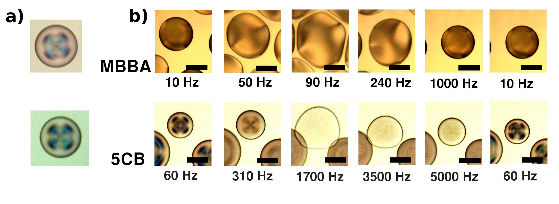
Figure 3: a) Images of nematic droplets of MBBA and 5CB dispersed in the isotropic phase in the absence of an applied electric field. b) In the series of images taken during frequency sweeps (sweep time: 100 s for MBBA: 10 Hz to 1 kHz and for 5CB: 50 Hz to 5 kHz, voltage 0.4 V/$\mu$m) the droplet shape and apparent size changes as a function of frequency. The scaling bar indicates 100 $\mu$m.

III Results

III.1 Colloid-free system

Figure 3 shows the results of typical frequency sweeps in MBBA and 5CB. Part a) shows field-free droplets, whereas in part b) all images were taken at 0.4 V/$\mu$m. Now, the director orientation in the droplets can be assumed to be predominantly perpendicular (MBBA) or parallel (5CB) to the optical path. In the absence of any applied field, there was no significant difference between MBBA and 5CB droplets. The observed texture of the droplets was consistent with spherically symmetric director orientation inside the droplets Ondris-Crawford et al. (1991).

When an electric field was applied, the texture of the MBBA droplets changed, as shown in Fig. 3. This was caused by the negative dielectric contrast $\Delta\epsilon$ of MBBA which leads to a predominantly in-plane director orientation. In the case of 5CB, the texture hardly change when turning on a low frequency field. This might be surprising since many of the material parameters (like the elastic constants) of the two samples are similar (see Tab. 1). In 5CB, however, the applied field did not change the symmetry along the optical path. Turning the director inside of the droplet parallel to the field and to the optical path keeps the rotational symmetry of the droplet projection through the microscope. This is different for MBBA, where the electric field turns the director perpendicular to the optical path and thus breaks the rotational symmetry of the projection image of the droplet.

		MBBA		5CB
Quantity		Value	Ref.	Value	Ref.
Interfacial tension	$\gamma$	$1.5\cdot 10^{-5}$ Nm-1	Williams (1976)	$1.6\cdot 10^{-5}$ Nm-1	Faetti and Palleschi (1984)
Dielectric constant	$\epsilon_{\parallel}$	4.85	Diguet et al. (1970)	15.5	Chandrasekhar (1977)
	$\epsilon_{\perp}$	5.1	Diguet et al. (1970)	7.5	Chandrasekhar (1977)
	$\epsilon_{iso}$	5	de Gennes and Prost (1993)	10.5	Chandrasekhar (1977)
Dielectric ratio	$S=\frac{\epsilon_{m}}{\epsilon_{d}}$	0.92		0.65
Electric conductivity	$\sigma_{m}$	$\mathit{5\cdot 10^{-8}}$ Sm-1		$\mathit{1.5\cdot 10^{-6}}$ Sm-1
Conductivity ratio	$R=\frac{\sigma_{d}}{\sigma_{m}}$	0.9	Diguet et al. (1970)	1.1	Jadzyn and Kêdziora (1987)
Viscosity ratio	$M=\frac{\nu_{m}}{\nu_{d}}$	2.1	Park et al. (1994)	0.7	Park et al. (1994)
Elastic constant	$K_{1}$	$6\cdot 10^{-12}$ N	Ivan (1972)	$6.2\cdot 10^{-12}$ N	Stewart (2004)
	$K_{2}$	$3.8\cdot 10^{-12}$ N	Ivan (1972)	$3.9\cdot 10^{-12}$ N	Stewart (2004)
	$K_{3}$	$7.5\cdot 10^{-12}$ N	Ivan (1972)	$8.2\cdot 10^{-12}$ N	Stewart (2004)

Table 1: Material parameters of MBBA and 5CB in the coexistence region. The electric conductivities were fitted to match the model with the experimental data as shown in Fig. 9. Still these values come within the limits typically expected for these materials. Note that $S$ is calculated for oriented droplets in which the director is perpendicular (MBBA) or parallel (5CB) to the applied field, with $\epsilon_{m}$ and $\epsilon_{d}$ being the dielectric constants of the continuous medium and the droplets, respectively.

Changing the frequency of the electric field not only changed the apparent size of the droplets, but also their internal texture, indicating a change of director orientation. In 5CB, this effect increased with frequency, corresponding to a good director orientation parallel to the field. In MBBA, the change was not visible due to the negative dielectric constant. From the evolution of the texture we can conclude that the higher the frequency,the better the orientation inside the droplets, i.e., the higher the electric field inside the sample.

All commercial liquid crystals have a small but finite conductivity based on ionic impurities. Since the electrodes are electrically insulated from the sample, we expect that the field in the sample is smaller than the applied electric field due to screening by ion migration. At low frequencies, the ions can easily follow the applied field and screen the sample, whereas at sufficiently high frequency, the limited ion mobility prevents this. Thus, the field is more markedly reduced at low than at high frequencies. The increase of the field as a function of frequency is responsible for the increasing orientation of the nematic droplets in 5CB as shown in Fig. 3b). In Sect. IV.1 we shall give a quantitative description of this effect.

As can be seen in Fig. 3b) (5CB) and in Fig. 4 (MBBA), the amplitude of the diameter change depends on the initial droplet size. In both 5CB and MBBA, droplets with an initial (field-free) diameter of 50 – 200 $\mu$m exhibited marked changes of the apparent size after field application. In MBBA, the amplitude ratio, i.e., the ratio of the maximum diameter to the initial diameter, varied from 1.2 for droplets initially 50 $\mu$m in diameter to values up to 2 for initial diameters of 140 $\mu$m and decreased again for even larger droplets. A similar behavior was observed in 5CB. Note that the frequency for the maximum diameter in 5CB is higher by about one order magnitude than in MBBA (see also Sect. IV).

Despite all these differences, the observed behavior was very similar in both systems. Furthermore, the samples could be used in many frequency sweeps (at least for several hours) without any noticeable change in the frequency response. The electrical insulation between the electrodes and the sample suppresses electrochemistry as a possible mechanism of degradation. However, the sample properties did change slightly in samples stored for more than 24 hours. For that reason, we only consider data taken within the first 5 hours after sample preparation. This virtually excludes field-induced damage as has been reported in experiments on electro-hydrodynamic convection (see, e.g., Richter et al. (1995)).

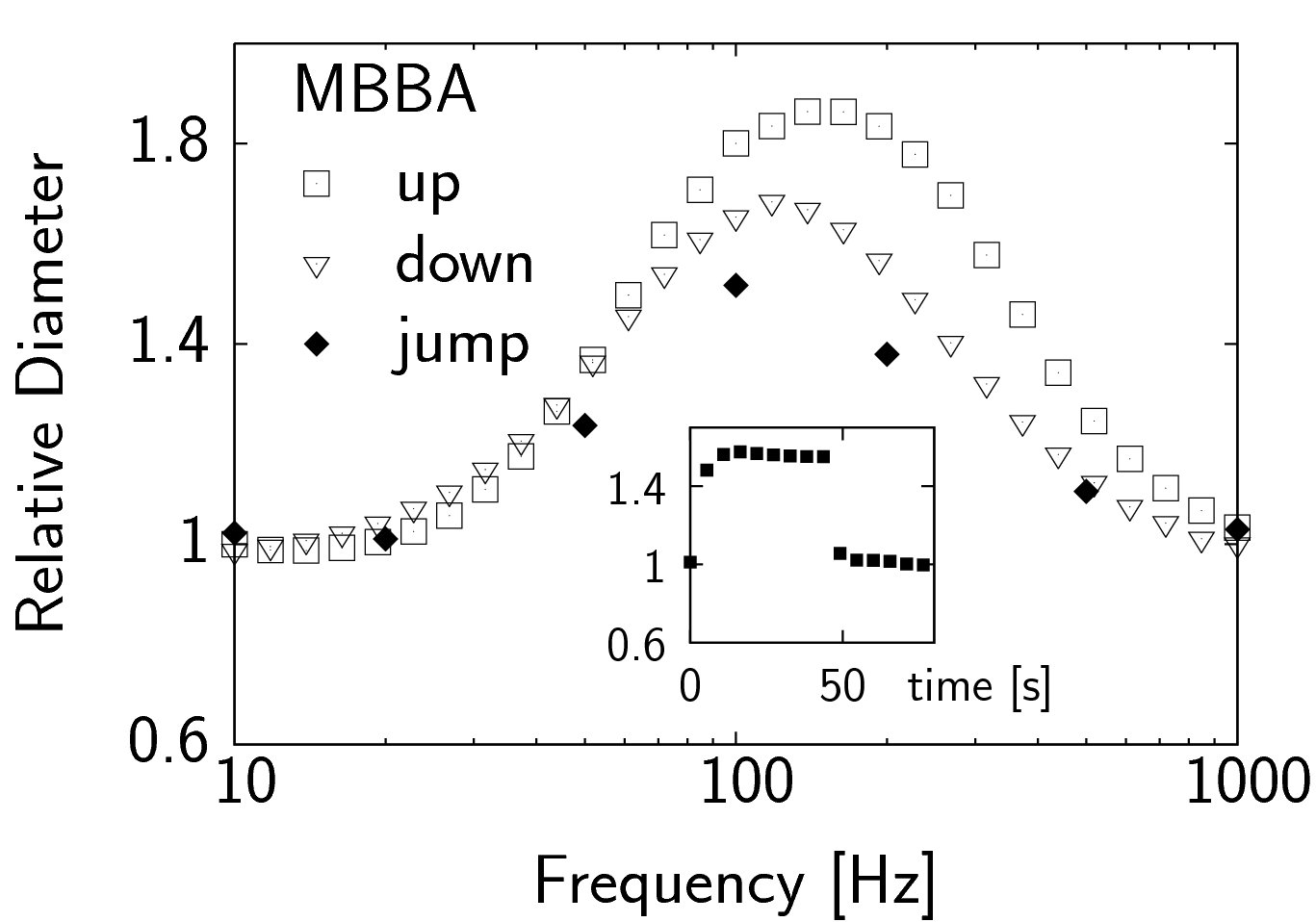
Figure 4: The typical evolution of MBBA droplets while changing the frequency in three different ways (up: logarithmic sweep from 10 Hz to 1 kHz; down: logarithmic sweep from 1 kHz to 10 Hz; jump: each frequency is directly addressed from a field free state). The apparent droplet diameters are normalized by their diameter before applying the field, which were measured to be 135 $\mu$m (up), 114 $\mu$m (down), and 91 $\mu$m (jump). The different amplitudes of the curves are due to the different initial droplet size. The sweeps in the major plot were performed with 100 s sweep time. The inset shows the time dependence of the relative diameter after turning on the voltage (jump at 100 Hz).

The shape change was almost independent of frequency history as shown for MBBA in Fig. 4. The amplitude variations are in the range expected for droplets of different size. However, the frequency of maximum amplitude $f_{max}$ was slightly less in the case of decreasing frequency sweeps. This indicates a small memory effect which might arise from ohmic heating in the ITO layers or from relaxation phenomena as shown in the inset to Fig. 4. After a jump in the applied voltage it takes 10 – 15 s until the droplet has attained its stable shape.

As temperature is kept constant, also the nematic volume fraction and droplet volume can be considered constant. Therefore, the observed increase in apparent diameter must be caused by flattening of the droplets, i.e., the droplets take an oblate (disk-like) shape with symmetry axis along the electric field (as sketched in Fig. 4). This behaviour differs from that predicted by purely dielectric considerations Taylor (1964).

III.2 Tracing the flow field

To test whether droplet deformation is of hydrodynamic origin, we added tracer colloids to the sample mixture prior to filling the chamber. In the coexistence region, these colloids remain exclusively in the isotropic part of the sample. Thus they visualize the flow field around the droplets.

These experiments revealed a strong flow within the isotropic phase around the nematic droplets. The tracer colloids moved outwards close to the droplet surface, turned upwards well inside the isotropic areas, returned above the droplet and then closed their convection role by moving downwards from above the droplet to its side at some distance from the interface. The resulting toroidal flow field is sketched in Fig. 5.

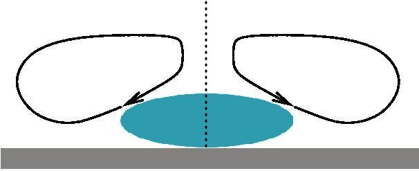
Figure 5: Sketch of the flow field around the nematic droplets as observed from tracer colloids. The flow field is axisymmetric around the center axis of the droplet (dotted line).

The projected velocity of the tracer colloids was highest close to the surface of the droplet. This indicates that the flow is driven by the interface (see Sect.IV for more details). Via viscous friction, the toroidal flow field leads to a net outward force on the droplet which leads to the transition from the spherical to the oblate droplet shape.

The velocity maximum at intermediate frequencies coincides with maximum deformation (Fig.6). Within the accuracy of the data, the flow velocity vanishes at high and low applied frequencies. Flow fields around droplets also lead to long-range interaction between the droplets Baygents et al. (1998). In our low surface tension system, this interaction leads to deviations from the circular shape, as shown in Fig. 3b).

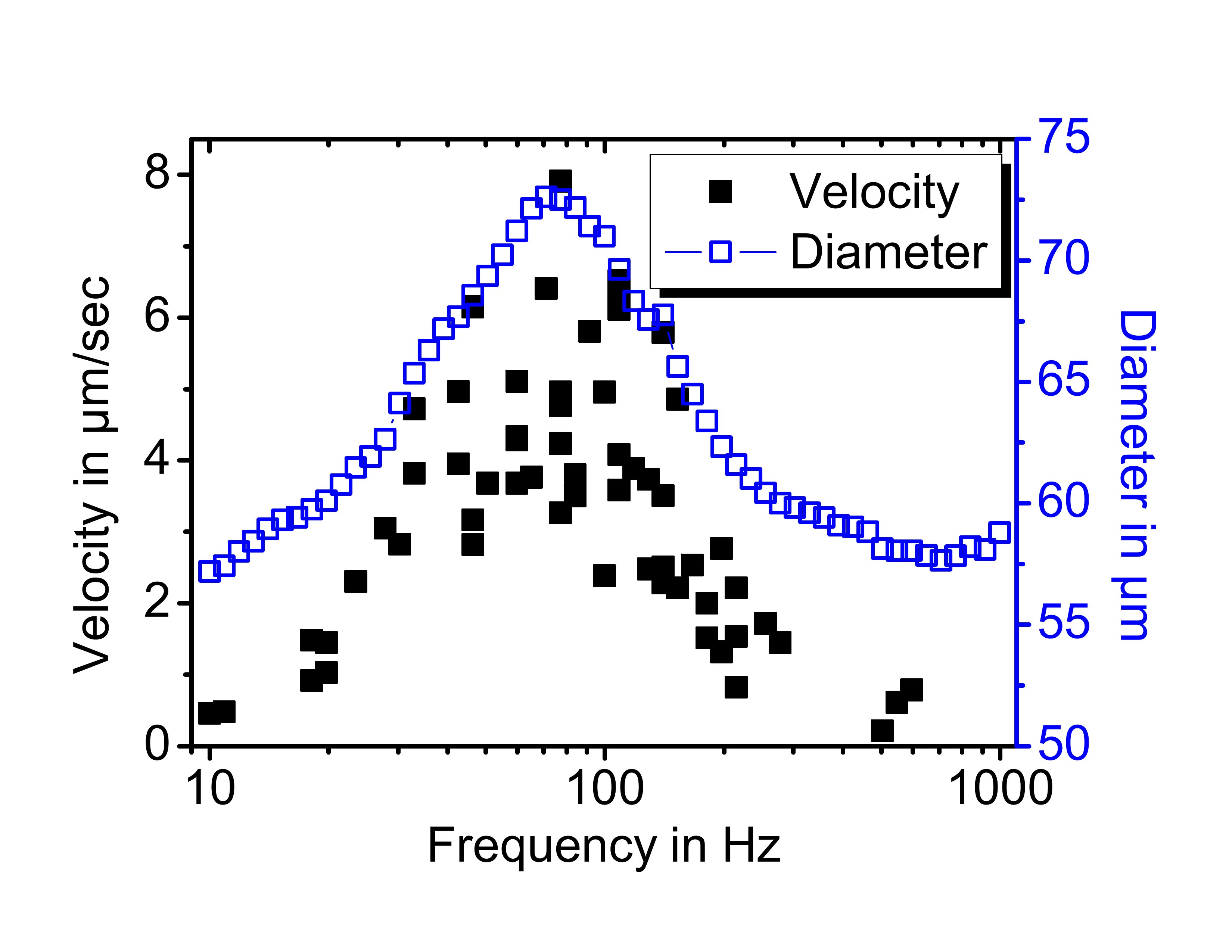
Figure 6: Characteristic flow velocities around a droplet (filled squares) and the corresponding apparent diameter of the droplet (open squares). To have a velocity measure which is independent from the actual droplet size, all flow velocities are measured at the perimeter of the maximum droplet size, i.e., for this droplet of a maximum diameter of 75 $\mu$m at about 40 $\mu$m from the droplet center.

IV Theoretical considerations

IV.1 Screening

To describe the screening of the electric field due to the finite conductivity of the sample, we use the model circuit sketched in the inset in Fig. 7. Here, we model the glass slides as pure capacitances, $C_{gl}$, and the sample as a capacitance, $C_{s}$, in parallel with an resistance, $R_{s}$ (assumed to be ohmic). The impedance ($Z_{cell}$) of this model circuit is given by the sum of the impedances of the glass slides, $Z_{gl}$, and the sample, $Z_{s}$

$$Z_{gl} = -\frac{i}{\omega C_{gl}}$$ (3)

$$Z_{s} = (\frac{1}{R_{s}}+i\omega C_{s})^{-1}$$ (4)

$$Z_{cell} = 2Z_{gl}+Z_{s},$$ (5)

with $i=\sqrt{-1}$, $\omega$ is the angular frequency of the applied field, the capacities given by $C=(\epsilon_{0}\epsilon A/d)$, the ohmic resistance $R_{s}=d/(A\sigma)$, the sample area by $A$, and the thickness $d=d_{gl}=d_{s}$. The voltage, $U_{s}$, actually applied to the sample given by

$$U_{s} = U_{0}\frac{Z_{s}}{Z_{cell}}$$ (6)

$$= U_{0}\frac{\omega\epsilon_{0}\epsilon_{gl}}{2\omega\epsilon_{0}\epsilon_{s}-2i\sigma+\omega\epsilon_{0}\epsilon_{gl}},$$

where $\epsilon_{0}=8.85\cdot 10^{-12}F/m$ is the permittivity of vacuum, $\epsilon_{s}$ and $\epsilon_{gl}$ are the dielectric constants of the glass slides and the sample, and $\sigma$ is the conductivity of the sample. Taking as typical values for MBBA $\epsilon_{s}=5$, $\sigma=0.5\cdot 10^{-7}S/m$, $\epsilon_{gl}=5$, and $U_{0}=200V$, we found that the voltage actually applied to the sample, $U_{s}$, reaches the value expected from purely dielectric considerations, $U_{s}^{dielect.}$ only for frequencies of a few hundred Hz (see also Fig. 7)

$$U_{s}^{dielect.}=U_{0}\frac{\epsilon_{gl}}{2\epsilon_{s}+\epsilon_{gl}}=\frac{U_{0}}{3}=\lim_{\frac{\sigma}{\omega}\to 0}U_{s}.$$ (7)

As expected, the sample is essentially field-free at low frequencies

$$\lim_{\omega\to 0}U_{s}=0.$$ (8)

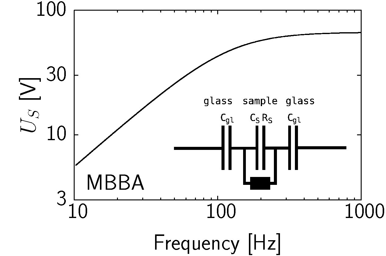
Figure 7: Modeling the effects of a small but finite conductivity of the samples. For typical values for MBBA ($\epsilon_{s}=5$, $\sigma=\sigma_{m}=0.5\cdot 10^{-7}S/m$, $\epsilon_{gl}=5$, and $U_{0}=200V$) the actual field in the sample reaches only at a few hundred Hz its purely dielectric value.

IV.2 Leaky dielectric model

The “leaky dielectric model” describes the behavior of a droplet immersed in an immiscible medium when subjected to an electric field. In this model, both the droplet and the continuous phase are assumed to be slightly conducting dielectrics. The foundations of that model have been laid by Taylor Taylor (1966), Torza Torza et al. (1971), Saville Vizika and Saville (1992); Saville (1997), and their coworkers. Recently this model has experienced more detailed experimental Bentenitis et al. (2005); Baygents et al. (1998) and numerical Fernádez et al. (2005); Zhang and Kwok (2005) verifications.

Here, we include a brief review of the leaky dielectric model (see the references cited above for details). Any electric current $\mathbf{j}$ induced by an applied field has to fulfill the continuity equation $\nabla\cdot\mathbf{j}=0$. Additionally, the electric field is submitted to the usual boundary conditions at the interface between the droplet and the medium $\nabla\cdot\epsilon\epsilon_{0}\mathbf{E}=\rho_{e}$ and $\nabla\times\mathbf{E}=0$. The combination of these conditions typically leads to a finite electrical charge density on the droplet surface.

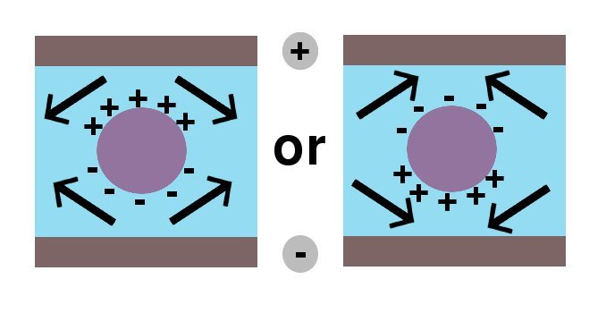
Figure 8: The combination of electric boundary conditions and continuity equation lead to surface charges on the droplet surface. These surface charges interact with the applied electric field and induce fluid motion tangential to the droplet surface.

As illustrated in Fig. 8, the interaction of these surface charges with the applied electric field induces electrokinetic effects, which ultimately lead to a fluid motion parallel to the droplet surface. Depending on the ratios of the conductivities, viscosities, and dielectric constants of both media, the flow above and below the droplet is directed outwards or inwards. Outward (inward) flow leads to an oblate (prolate) deformation of the droplet. The deformation consists of a stationary and a time-dependent part. The amplitude of the latter turned out to be below the detection limit of our set-up, i.e., is negligible in our system. In the notation adopted by Saville and coworkers Vizika and Saville (1992); Saville (1997), the stationary deformation of the droplet $D_{s}=(d_{1}-d_{2})/(d_{1}+d_{2})$ (with $d_{1}$ and $d_{2}$ being the principal diameters of the droplet) can be expressed by

$$D_{stat}=\frac{9}{16}\epsilon_{0}\epsilon_{m}\frac{aE^{2}}{\gamma}\Phi,$$ (9)

with $a$ representing the droplet radius in the absence of an electric field and $E$ the actual field in the sample. Since the interfacial tensions $\gamma$ enters in the denominator, it is clear that the extremely small value of $\gamma\approx 1.5\cdot 10^{-5}$ N/m enables large deformation of the droplets. The function $\Phi$ determines the type of the deformation. It is positive (negative) for prolate (oblate) droplets

$$\Phi=1-\frac{S^{2}R(11+14M)+15S^{2}(1+M)+S(19+16M)+R^{2}S\tau\omega(M+1)(S+2)}{5(M+1)[S^{2}(2+R)^{2}+R^{2}\tau^{2}\omega^{2}(1+2S)^{2}]}.$$ (10)

Here, $R=\sigma_{d}/\sigma_{m}$ denotes the ratio of the conductivities, $S=\epsilon_{m}/\epsilon_{d}$ the ratio of the dielectric constants, $M=\nu_{m}/\mu_{d}$ the ratio of the viscosities, $\tau=\epsilon\epsilon_{0}/\sigma$ the characteristic time, $\omega$ the angular frequency of the applied electric field, and indices $d$ and $m$ indicate the properties of the droplet and the continuous medium, respectively. $\Phi$ is a monotonic function of $\omega$ which may change sign as a function of $\omega$, but has no maximum or minimum at finite $\omega$. To obtain a maximum in the deformation we have to include the frequency dependent electric field in the sample discussed above.

IV.3 Comparison with our data

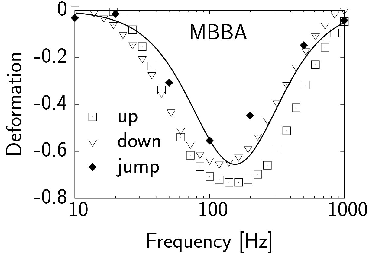
Figure 9: The deformation $D_{s}=(d_{1}-d_{2})/(d_{1}+d_{2})$ (with $d_{1}$ and $d_{2}$ being the principal diameters of the droplet) as calculated from the data of Fig. 4 (assuming a constant droplet volume) is compared to the combination of screening and the leaky dielectric model (solid line). The modelling curve has been calculated with the material parameters given in Tab. 1, an applied ac voltage with 200 V amplitude, a droplet radius of 60 $\mu$m, and an electrode distance of 500 $\mu$m.

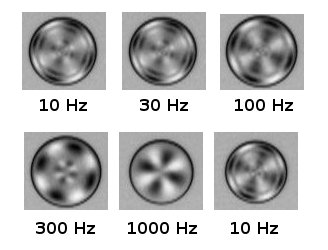
Figure 10: Frequency dependent deformation of nematic droplets in a 5CB/ionic liquid mixture (about 0.01 vol% of 1-butyl-3-methylimidazolium trifluoromethansulfonimid in 5CB).

The solid line in Fig. 9 combines our estimate of the actual voltage applied to the sample, $E_{s}=U_{s}/d$ from Eq.(6), with the frequency dependent deformation given by Eq. (10). In this comparison we used the material parameters (see Tab. 1) given in the literature and chose the value of the only free parameter in the model, the conductivity, to fit the measured deformations. The resulting values for the conductivity ($\sigma_{MBBA}=5\cdot 10^{-8}$ S/m and $\sigma_{5CB}=1.6\cdot 10^{-6}$ S/m) are in the range expected for liquid crystals. With the above assumptions, the combination of leaky dielectric model and screening due to the finite conductivity accurately describes the measured data.

To verify the effect of free charges, we increased the concentration of free ions by mixing one of the samples (5CB) with an ionic liquid (1-butyl-3-methylimidazolium trifluoromethansulfonimide). This strongly suppressed all field-induced effects. At a concentration of a few vol% neither a change in texture nor a deformation was observed. Even at much lower charge concentrations, both effects were detectable but partially suppressed compared to pure samples (see Fig. 10). We attribute this strong reduction to the high concentration of free ions which leads to a significantly higher conductivity and thus to better screening.

V Conclusion

The extremely low interfacial tension at the nematic-isotropic interface allows for easy deformation of nematic droplets in the isotropic-nematic coexistence interval.

The reported frequency-dependent oblate (disc-like) deformation of nematic droplets induced by an applied electric ac field extents the behaviour expected in ”leaky” dielectrics. A part from the anisotropy in the material parameters, the nematic degrees of freedom seem not to play a significant role in mechanisms leading to the droplet deformation. Working with insulated electrodes suppressed electrochemical reactions at the electrodes but also made it necessary to include screening in the theoretical description. As characteristic for leaky dielectrics, an interface-driven, frequency-dependent hydrodynamic flow field around the droplets was induced by the electric field. The effective field however was reduced due to screening by field-induced charges at the interface, caused by the finite conductivity of the sample. Accordingly, combining screening with the ”leaky dielectric” model accurately describes the experimentally observed droplet deformation.

References

- Crawford and Zumer (1996) (Eds.) G. P. Crawford and S. Zumer (Eds.), Liquid Crystals in Complex Geometries (Taylor and Francis, London, UK, 1996).
- Candau et al. (1973) S. Candau, P. Le Roy, and F. Debeauvais, Mol. Cryst. Liq. Cryst. 23, 283 (1973).
- Doane et al. (1986) J. W. Doane, N. A. Vaz, B.-G. Wu, and S. Zumer, Appl. Phys. Lett. 48, 268 (1986).
- Chan (1999) P. K. Chan, Liquid Crystals 26, 1777 (1999).
- Lubensky et al. (1998) T. C. Lubensky, D. Pettey, N. Currier, and H. Stark, Phys. Rev. E 57, 610 (1998).
- Dolganov et al. (2007) P. V. Dolganov, H. T. Nguyen, G. Joly, V. K. Dolganov, and P. Cluzeau, Europhys. Lett. 78, 66001 (2007).
- Park et al. (1994) C. S. Park, N. A. Clark, and R. D. Noble, Phys. Rev. Lett. 72, 1838 (1994).
- Lev et al. (2001) B. I. Lev, V. G. Nazarenko, A. B. Nych, D. Schur, P. M. Yamamoto, and H. Yukuyama, Phys. Rev. E 64, 021706 (2001).
- Wu et al. (2007) Y. Wu, W. Yu, C. Zhou, and Y. Xu, Phys. Rev. E 75, 041706 (2007).
- El-Sadek et al. (2007) R. El-Sadek, M. Roushdy, and J. Magda, Langmuir 23, 7907 (2007).
- Coates (1995) D. Coates, J. Mater. Chem. 5, 2063 (1995).
- Bouteiller and LeBarny (1996) L. Bouteiller and P. LeBarny, Liq. Cryst. 21, 157 (1996).
- Bunning et al. (2000) T. J. Bunning, L. V. Natarajan, V. P. Tondiglia, and R. L. Sutherl, Ann. Rev. Mater. Sci. 30, 83 (2000).
- Tjong (2003) S. Tjong, Mater. Sci. Eng. Reports 41, 1 (2003).
- Jeon et al. (2007) Y. J. Jeon, Y. Bingzhu, J. T. Rhee, D. L. Cheung, and M. Jamil, Macromol. Theory Simul. 16, 643 (2007).
- Chiu and Kyu (1995) H.-W. Chiu and T. Kyu, J. Chem. Phys. 103, 7471 (1995).
- Shen and Kyu (1995) C. Shen and T. Kyu, J. Chem. Phys. 102, 556 (1995).
- Lin et al. (1998) Z. Lin, H. Zhang, and Y. Yang, Phys. Rev. E 58, 5867 (1998).
- DasGupta et al. (2001) S. DasGupta, P. Chattopadhyay, and S. K. Roy, Phys. Rev. E 63, 041703 (2001).
- Mukherjee (2002) P. K. Mukherjee, J. Chem. Phys. 116, 9531 (2002).
- Langevin and Bouchiat (1973) D. Langevin and M. A. Bouchiat, Mol. Cryst. Liq. Cryst. 22, 317 (1973).
- Faetti and Palleschi (1984) S. Faetti and V. Palleschi, Phys. Rev. A 30, 3241 (1984).
- Williams (1976) R. Williams, Mol. Cryst. Liq. Cryst. 35, 349 (1976).
- Yokoyama et al. (1985) H. Yokoyama, S. Kobayashi, and H. Kamei, Mol. Cryst. Liq. Cryst. 129, 109 (1985).
- Roussel et al. (2000) F. Roussel, J.-M. Buisine, U. Maschke, X. Coqueret, and F. Benmouna, Phys. Rev. E 62, 2310 (2000).
- Ullrich et al. (2006) B. Ullrich, E. Ilska, N. Höhn, and D. Vollmer, Prog. Colloid. Polym. Sci. 113, 142 (2006).
- Antl et al. (1986) L. Antl, J. W. Goodwin, R. D. Hill, R. H. Ottewill, S. M. Owens, S. Papworth, and J. A. Waters, Colloids and Surfaces 17, 67 (1986).
- Bosma et al. (2002) G. Bosma, C. Pathmamanoharan, E. H. A. de Hoog, W. K. Kegel, A. van Blaaderen, and H. N. W. Lekkerkerker, Journal of Colloid and Interface Science 245, 292 (2002).
- Deschamps et al. (2008) J. Deschamps, J. P. M. Trusler, and G. Jackson, J. Phys. Chem. B 112, 3918 (2008).
- Ondris-Crawford et al. (1991) R. Ondris-Crawford, E. P. Boyko, B. G. Wagner, J. H. Erdmann, S. Zumer, and J. W. Doane, J. Appl. Phys. 69, 6380 (1991).
- Diguet et al. (1970) D. Diguet, F. Rondelez, and G. Durand, C. R. Acad. Sci. Paris B 271, 954 (1970).
- Chandrasekhar (1977) S. Chandrasekhar, Liquid crystals (Cambridge University Press, Cambridge, UK, 1977).
- de Gennes and Prost (1993) P. G. de Gennes and J. Prost, The Physics of Liquid Crystals (Clarendon Press, Oxford, 1993).
- Jadzyn and Kêdziora (1987) J. Jadzyn and P. Kêdziora, Mol. Cryst. Liq. Cryst. 145, 17 (1987).
- Ivan (1972) H. Ivan, The Journal of Chemical Physics 57, 1400 (1972).
- Stewart (2004) I. W. Stewart, The static and dynamic continuum theory of liquid crystals (Taylor and Francis, London, 2004).
- Richter et al. (1995) H. Richter, A. Buka, and I. Rehberg, Phys. Rev. E 51, 5886 (1995).
- Taylor (1964) G. Taylor, Proc. R. Soc. Lond. A 280, 383 (1964).
- Baygents et al. (1998) J. C. Baygents, N. J. Rivette, and H. A. Stone, J. Fluid Mech. 368, 359 (1998).
- Taylor (1966) G. Taylor, Proc. R. Soc. Lond. A 291 (1966).
- Torza et al. (1971) S. Torza, R. G. Cox, and S. G. Mason, Phil. Trans. R. Soc. Lond. A 2969, 295 (1971).
- Vizika and Saville (1992) O. Vizika and D. A. Saville, 239, 1 (1992).
- Saville (1997) D. A. Saville, Annu. Rev. Fluid Mech. 29, 27 (1997).
- Bentenitis et al. (2005) N. Bentenitis, S. Krause, and K. Benghanem, Langmuir 21, 790 (2005).
- Fernádez et al. (2005) A. Fernádez, G. Tryggvason, J. Che, and S. L. Ceccio, Phys. Fluids 17, 093302 (2005).
- Zhang and Kwok (2005) J. Zhang and D. Y. Kwok, J. Comput. Phys.. 206, 150 (2005).