Generalized fluctuation-dissipation relation and effective temperature
in off-equilibrium colloids

Abstract

The fluctuation-dissipation relation (FDR), a fundamental result of equilibrium statistical physics, ceases to be valid when a system is taken out of the equilibrium. A generalization of FDR has been theoretically proposed for out-of-equilibrium systems: the kinetic temperature entering FDR is substituted by a time-scale dependent effective temperature. We combine the measurements of the correlation function of the rotational dynamics of colloidal particles obtained via dynamic light scattering with those of the birefringence response to study the generalized FDR in an off-equilibrium clay suspension undergoing aging. We i) find that FDR is strongly violated in the early stage of the aging process and is gradually recovered as the aging time increases and, ii), we determine the aging time evolution of the effective temperature, giving support to the proposed generalization scheme.

The study of the dynamics in non-equilibrium systems is an intriguing and fascinating area of modern physics. There is an obvious interest in the off-equilibrium regime as condensed matter is often found far from ideal equilibrium condition. In these cases where “things keep happening on all time scales” Fey some of the most fundamental symmetries of equilibrium statistical mechanics are broken. A particular class of systems where the out-of-equilibrium status occurs naturally are the so called glass forming systems. These systems include, for example, disordered spin systems close to the spin-glass transition, supercooled molecular liquids, and jamming colloidal solutions. In general the dynamics of these systems is extremely sensitive to change of external parameters so that, when they are a little cooled or densified, the time required to re-establish equilibrium grows enormously and an off-equilibrium regime is entered. Here the average quantities becomes time dependent and the correlation and response functions depend on two times, in this regime the system is known to perform aging).

Correlation functions and response functions are the basic quantities through which one probes the dynamics of a system in many-body statistical physics. These functions are closely related in equilibrium by the fluctuation-dissipation theorem (FDT). The FDT Hansen establishes a relationship between the correlation function $C_{AB}(t)=\langle A(0)B(t)\rangle$ of the spontaneous equilibrium fluctuations of the dynamic variables $A$ and $B$ and the response function $\chi_{AB}(t)=\langle A(t)\rangle/h$, describing the change in the average value of $A$ due to an infinitesimal external field $h$ that is coupled to the variable $B$ in the perturbation Hamiltonian:

$$\chi_{AB}(t)=\beta\left[C_{AB}(0)-C_{AB}(t)\right].$$ (1)

Here $\beta=1/k_{B}T$, where $T$ is the kinetic temperature of the system and $A$ and $B$ are variables that have zero-mean in the unperturbed case. In this formulation of the FDT the field $h$ introduces an energy contribution $\delta H=-hB$ in the system Hamiltonian and it is switched on instantaneously at $t=0$ and kept constant for $t>0$ as an Heaviside step-function. In the following we will refer to auto-correlation function ($B=A$) and drop the label $AA$ in $C_{AA}(t)$ and $\chi_{AA}(t)$.

Out of equilibrium the system is non-stationary and time-translational invariance is lost. The correlation and the response become two-times quantities depending also on the aging time $t_{w}$: $C=C(t_{w},t_{w}+t)$, $\chi=\chi(t_{w},t_{w}+t)$ and the FDT (1) is not supposed to hold. The importance of extending the theorem to the non-equilibrium regime has led to propose the generalized fluctuation-dissipation relation (GFDR) Crisanti ; Vulpiani ; Cugliandolo .

The generalization of the FDT proposed by Kurchan and Cugliandolo Kurchan ; Kurchan2 in the early ’90 can be expressed as follows:

$$\chi(t_{w},t_{w}+t)=\beta\int_{t_{w}+t}^{t_{w}}dsX(t_{w},s)\partial_{s}C(t_{w},s)$$ (2)

where for short times $t$ (i.e. $t/t_{w}\ll 1$) the previous equation reduces to the FDT (Eq. 1) and the system is said to be in a quasi-equilibrium state; for intermediate $t$ ($t/t_{w}\simeq 1$) the violation function $X(t_{w},t)$ quantifies the deviation of the GFDR from the FDT; finally, when $t/t_{w}\gg 1$, the function $X$ depends on $t_{w}$ and $s$ only through the function $C$. The violation function can also be interpreted theoryofTeff ; detailedTeff in terms of an effective temperature $T_{eff}=T/X$. The latter has complicated behavior for intermediate $t$ values, but in the long-$t$ regime it assumes a value that depends only on the waiting time $t_{w}$ and one can think of it as ”waiting-time dependent effective temperature”.

The GFDR in out-of-equilibrium systems has been studied theoretically and through computer simulations in spin-glasses SpinGlasses ; Mezard and in models for glassy dynamicsGregor . Later, off-equilibrium molecular dynamics simulations have given the possibility to perform the same analysis on structural glasses Parisi1 ; Sellitto ; Kob ; Di Leonardo . Recently the generalized relation has also been investigated in more exotic systems, like in the simulations for a glassy protein bio , in self-assembling processes of viral capsids formation and of sticky disks crystallization virdis and in active systems composed of self-propelled particles active .

On the other hand few experiment have attempted to study the GFDROcio ; Grigera ; Bellon ; Jabbari ; Greinert ; Ciliberto2 ; CilibertoNew . Furthermore the results reported until now for structural glasses remain controversialGrigera ; Bellon ; Jabbari ; Greinert ; Ciliberto2 . The experiments in structural glasses are intrinsically difficult because it is necessary to simultaneously measure a correlation function of a given variable and the associated response function, and all this in a systems that is instantaneously brought out-of equilibrium. These difficulties are relaxed in the case of colloidal glasses (or gels, or jams), because the associated timescales are much longer and fall easily in the experimentally accessible window.

In this letter we report an experimental investigation of the generalized FDR in a colloidal systems composed of a water suspension of clay platelets (Laponite), which is off equilibrium when it ages towards the final arrested state (gel or glass, depending on the clay concentration BR ). We study the reorientational dynamics of the asymmetric clay platelets, looking at the orientational correlation functions via depolarized dynamic light scattering and at the corresponding response function via the electric field induced birefringence. Measuring both $C=C(t_{w},t_{w}+t)$ and $\chi=\chi(t_{w},t_{w}+t)$ at different waiting time during the (days long) aging process we find that FDR is strongly violated in the early stage of the aging process and is gradually recovered as the aging time increases. Moreover, from the parametric $C-\chi$ plot (the so called ”FDT plot”) we determine the effective temperature and follow its evolution from the high values ($T_{eff}/T\approx 5$) pertaining to young systems towards the equilibrium ($T_{eff}/T=1$) attained at long waiting time. Our findings confirm the generalization of the FDT to off-equilibrium systems proposed by Cugliandolo and Kurchan 15 year ago.

The off-equilibrium sample. A solution, prepared by stirring the Laponite powder with water, evolves toward an arrested state on a timescale that span the ranges hours to months when simply kept at room temperature and pressure. Even low concentration aqueous solutions of this colloid, as the one used in our experiment ($\sim 1$ % Laponite weight fraction), show strong aging of its light-scattering correlation function Laura . Due to its long (with respect to the experimental timescale and to the decorrelation time) aging process of the systems, one can approximate the different measure of fluctuations and response as obtained in a sequence of steady out of equilibrium states. Furthermore, the anisotropic shape of the clay disc makes it possible to study its reorientation dynamics through the response and the correlation function. Laponite particles dissolved in water have the form of flat cylinders with a diameter of 25 nm and an thickness of about 1 nm. Laponite colloidal particles are good scatterers of visible light and this allow us to rapidly measure the autocorrelation function of the scattered field.

The correlation function. In a dynamic light scattering experiment one measures the correlation function of the optical field scattered by the sample. The scattered field can be directly related to the translational and rotational motion of the anisotropic colloids suspended in the solvent Pecora . The colloid’s rotations are related to the second rank tensor of the optical susceptibility. Specifically, in the VH (depolarized) scattering geometry, one measures the autocorrelation function of a variable that depends on the platelet’s orientation:

$$A(t)=\sum_{i}P_{2}(\cos(\theta_{i}(t)))$$ (3)

where $P_{2}(x)=(3x^{2}-1)/2$ is the 2nd order Legendre polynomial, $\theta_{i}$ is the angle formed by the symmetry axes of the $i$-th particle with the polarization vector of the incident field and the sum is extended over the particles contained in the scattering volume Pecora . This results holds exactly only if the time scale of the rotational dynamics is much faster than the translational one. This assumption was confirmed by comparing the VV (polarized) and VH (depolarized) photon correlation (PCS) at different waiting times and clay concentration Supp . The autocorrelation function of $A$ was measured using the VH geometry via PCS. Several autocorrelation functions have been measured during the aging process of the sample with a time resolution (1 $\mu$s) dictated by the time-structure of the detector (photomultiplier) response.

The response function. If one applies an external field that tend to align the particle the system -due to the anisotropic platelet’s polarizability- becomes birefringent Boyd ; Hecht . If the aligning field is a DC (or low frequency) electric field (Kerr effect) the degree of rotation of a linearly polarized laser beam is proportional to the square of the electric field via a coefficient that is proportional to $A$ (Eq. 3). Therefore, the (time dependent) Kerr response to the switch-on of an electric field is proportional to the desired response function (i.e. the response conjugated to the correlation function measured in depolarized PCS). For selected values of the waiting times, the time resolved response functions and the corresponding correlation functions, was measured during the aging process of the Laponite solution. The length of the electric pulses produced sets the dynamic window of our experiment to about 1 ms.

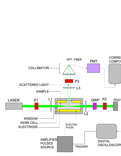
Figure 1: Sketch of the experimental set-up (see Ref.Supp for more details). The laser’s radiation ($\lambda=532$ nm) is polarized by the polarizer P1 and focused by the lens L1 at the centre of the cell containing the sample. The scattered light is collected by the lens L3 and selected by the polarizer P3 (orthogonal to P1). A photo-multiplier tube (PMT) detect the scatterd photons. When no electric pulse is applied to the cell the output of the PMT is acquired by a computer equipped with a custom digital correlator, this measures and stores the correlation function. The Kerr-cell containing the sample is provided by two electrodes connected to a source of amplified electric pulses. The forward-scatterd light (rotated by the electrically stimulated sample) is collected by the lens L2 and passes through a quarter-wave plate (QWP) and the polarizer P2 (orthogonal to P1). The transmitted light is detected by a photodiode connected to a digital oscilloscope. This is triggered to the source of electric pulse measuring and storing the Kerr-response function.

Note that the relaxation time $\tau$ of these functions is always much smaller that the typical waiting time ($\tau\ll t_{w}$). This means that the time-resolved correlation and response are well-defined quantities although the system is aging. In addition, if any FDT-violation can be detected, we expect to find that in on a timescale comparable to the relaxation time ($t/\tau\geq 1$).

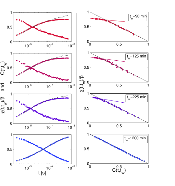
Figure 2: (Left) Normalized time correlation function ($\circ$) and response function ($\Box$) measured at different aging times (from top to bottom: $t_{w}=90$, 125, 225 and 1200 min), the solid line represents $1-C$. Note that $1-C$ deviates from $\chi/\beta$ when the FDT is violated. The importance of this deviation reduces as $t_{w}$ increases. (Right) Response function vs correlation function measured at different aging times ($\circ$), the black line represents the expectation of the FDT while the color lines represent the linear fits to the points in the off-equilibrium section of the FDT plot. It can be appreciated how these points corresponding to long times approach gradually the FDT as the aging time increases, for the longest waiting time the fitting line overlaps almost perfectly with the prediction of the FDT (see Fig. 3 for a comparison of the FDT plots at different aging times).

Examples of the measured quantities are shown in the left panel of Fig. 2. The correlation function and the response function are reported as functions of $t$ for different aging times $t_{w}$. For short $t$ the FDT holds while we can see a clear deviation from the FD relation for long $t$ where $\chi/\beta$ does not overlap with $1-C$ ($C(t)$ is normalized to $C(0)=1$). When $\chi(t_{w},t_{w}+t)/\beta$ is parametrically plotted against $C(t_{w},t_{w}+t)$ using $t$ as parameter (FDT plot) the departure from the $1-C$ line becomes evident (see the right panel of Fig. 2). The deviation from the behavior expected from the FDT reduces its importance as $t_{w}$ grows, and the time where $T\chi$ and $C$ detaches from each other moves to longer $t$ (see also Fig. 3(a), where the interested region of the FDT plot has been expanded). In order to quantify this deviation, we have performed a straight line fit to the longer time points in the FDT plot. The slopes ($m$) of these lines are a measure of the effective temperature: $1/m=T_{eff}/T$.

The $t_{w}$ dependence of $T_{eff}$ is reported in Fig. 3(b): $T_{eff}$ decreases as $t_{w}$ increases. The linear fit to the long $t$ region of the FDT plot also defines a characteristic value of the correlation $C$ where the FDR breaks-down, the so called Edwards-Anderson value $q$; this quantity is reported as a function of $t_{w}$ in Fig. 3(c). Finally, the quantity $q$, via $C(t_{o})=q$, identifies a characteristic time $t_{o}$ that mark the ”starting time” of the violation. $t_{o}$ is found to move to higher values as the aging time increases (Fig. 3(d)). It is interesting to compare $t_{o}$ to the relaxation times $\tau$ of the response and the correlation. We find $\tau$ fitting the correlation and the response with stretched exponential of the form $\exp[-(t/\tau)^{\beta}]$ and $(1-a\,\exp[-(t/\tau)^{\beta}])$, respectively. The response ages faster than the correlation almost reaching the same relaxation time for the longest $t_{w}$.

It is important to emphasize that in all models investigated so far, for studying the generalization of the FDR, the relaxation time grows roughly as the waiting time: $\tau\sim t_{w}$. The aging process that we study experimentally here does not obey this simple scaling, the relaxation time being several orders of magnitude shorter than the typical values of $t_{w}$. Nevertheless the findings that we report in this work indicate that the generalized form of theorem applies if $t/t_{w}$ is replaced by $t/\tau$ in marking the transition of the different interesting regions.

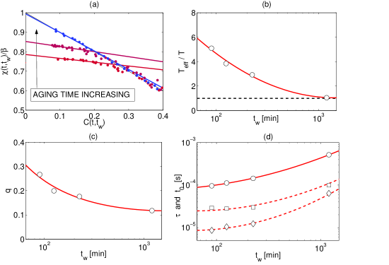
Figure 3: (a) The interesting region of the FDT plots for different aging times: $t_{w}=90$, 125 and 1200 min (cfr. Fig. 2, right panel). (b) The inverse slope of the long times points of the FDT plot (see Fig . 2) as a function of the aging time, the red line is a guide for the eye. This parameter can be interpreted as an effective temperature and it is found to reduce to the bath temperature as the aging time increases. (c) Waiting time dependence of the Edwards-Anderson parameter, the characteristic value of the correlation function at which the FDT breaks-down. (d) Evolution with $t_{w}$ of the characteristic time at which the FDT is violated ($\circ$), together with the relaxation time of the correlation function ($\Box$) and of the response ($\diamondsuit$). The characteristic time for the FDT violation $t_{o}$ increases as $t_{w}$ grows followed by the two relaxation times.

In conclusion, by measuring the autocorrelation function of a given variable and the response function of the same quantity in an off-equilibrium (aging) colloidal suspension in the route to the arrested state, we have tested the validity of the generalized fluctuation-dissipation relation. The prediction of the GFDR apply to the present experiment, and on the probed time-scale we observe that the deviation from the satndard FDT reduces gradually as the arrested phase is approached. The characteristic time at which the violation is seen is always slightly above the relaxation time of the measured response and correlation function.

References

- (1) R. P. Feynman. Statistical mechanics: a set of lectures. notes taken by R. Kikuchi. Jacob Shaham (Academic Press 1972).
- (2) see for example the textbooks: J.-P. Hansen and I.R. McDonald. Theory of Simple Liquids, 3rd edition Chap. 7. (Academic Press 2006), L. D. Landau and E. M. Lifshitz. Statistical Physics: Volume 5. (Butterworth-Heinemann 1980), D. Chandler. Introduction to Modern Statistical Mechanics (Oxford University Press 1987).
- (3) A. Crisanti and R. Ritort. J. Phys. A 36, R181 (2003).
- (4) U. M. Marconi, A. Puglisi, L. Rondoni and A. Vulpiani Phys. Rep. 461, 111 (2008).
- (5) L. F. Cugliandolo Slow Relaxations and nonequilibrium dynamics in condensed matter Course 7: Dynamics of Glassy Systems (Springer Berlin / Heidelberg 2004).
- (6) L.F. Cugliandolo and J. Kurchan. Phys. Rev. Lett. 71, 173 (1993).
- (7) L.F. Cugliandolo and J. Kurchan. J. Phys. A 27, 5749 (1994).
- (8) L. F. Cugliandolo et al. Phys. Rev. E 55, 3898 (1997).
- (9) Garriga and F. Ritort. Eur. Phys. J. B 21, 115 2001).
- (10) M. Mézard, G. Parisi and M. A. Virasoro Spin Glass theory and Beyond. World Scientific, Singapore (1987).
- (11) J. Kurchan, J. P. Bouchard et al. Spin Glasses and Random Fields World Scientific, Singrapore (2000).
- (12) G. Diezemann. J. Chem. Phys. 123, 204510 (2005).
- (13) G. Parisi. Phys. Rev. Lett. 79, 3660 (1997).
- (14) M. Sellitto, Eur. Phys. J. B 4, 135 (1998)
- (15) W. Kob and J. L. Barrat. Eur. Phys. Lett. 46, 637 (1999);
- (16) R. Di Leonardo, L. Angelani, G. Parisi, and G. Ruocco. Phys. Rev. Lett. 84, 6054 (2000).
- (17) K. Hayashi and M. Takano. Biophys. Journal 93, 895 (2007).
- (18) R. L. Jack, M. F. Hagan and D. Chandler. Phys. Rev. E 76, 021119 (2007).
- (19) D. Loi, S. Mossa and L. F. Cugliandolo. Phys. Rev. E 77, 051111 (2008)
- (20) D. Herisson and M. Ocio. Phys. Rev. Lett. 88, 257202 (2002).
- (21) T. S. Grigera and N. Israeloff. Phys. Rev. Lett. 83, 5038 (1999).
- (22) L. Bellon, S. Ciliberto and C. Laroche. Europhys. Lett. 53, 511 (2001).
- (23) S. Jabbari-Farouji et al. Phys. Rev. Lett. 98, 108302 (2007).
- (24) N. Greinert et al. Phys. Rev. Lett. 97, 265702 (2006).
- (25) P. Jop, A. Petrosyan, and S. Ciliberto. Phil. Mag. 88, 4205 (2008).
- (26) J. R. Gomez-Solano, A. Petrosyan, S. Ciliberto, et al. arXiv:0903.1075 [cond-mat.stat-mech] (2009).
- (27) B. Ruzicka, L. Zulian, R. Angelini et al. Phys. Rev. E 77, 020402 (2008).
- (28) B. Berne, and R. Pecora. Dynamic Light Scattering. Plenum, New York (1985).
- (29) C. Maggi Auxiliary Material. (2008).
- (30) B. Ruzicka, L. Zulian and G. Ruocco. Langmuir 22 (3), 1106 (2006).
- (31) R. W. Boyd. Nonlinear Optics. Academic Press, San Diego (2003).
- (32) E. Hecht. Optics (4th edition). Addison Wesley (2001).