On the spectrum of fluctuations of a liquid surface:
From the molecular scale to the macroscopic scale

Abstract

We show that to account for the full spectrum of surface fluctuations from low scattering vector $qd\!\ll\!1$ (classical capillary wave theory) to high $qd\!\apprge\!1$ (bulk-like fluctuations), one must take account of the interface’s bending rigidity at intermediate scattering vector $qd\!\apprle\!1$, where $d$ is the molecular diameter. A molecular model is presented to describe the bending correction to the capillary wave model for short-ranged and long-ranged interactions between molecules. We find that the bending rigidity is negative when the Gibbs equimolar surface is used to define the location of the fluctuating interface and that on approach to the critical point it vanishes proportionally to the interfacial tension. Both features are in agreement with Monte Carlo simulations of a phase-separated colloid-polymer system.

I Introduction

The description of the spectrum of surface fluctuations of a liquid from the macroscopic scale down to the molecular scale remains a challenging experimental and theoretical problem. Using grazing incidence light scattering experiments, Daillant and coworkers Daillant were able, for the first time, to determine the full spectrum of surface fluctuations, where in previous experiments (ellipsometry, reflectivity) only certain aspects of the spectrum could be determined. At the same time, the spectrum can now be analyzed in computer simulations with ever increasing accuracy Stecki ; Vink ; Tarazona .

Theoretical insight into the structure of a simple liquid surface is provided by density functional theories on the one hand Evans ; Henderson ; RW and the capillary wave model on the other hand BLS ; Weeks ; Bedeaux . Density functional theories provide a description of the interface on a microscopic level. The prototype of such theories, the van der Waals squared-gradient model, was very successful in describing, for the first term, the density profile and surface tension in terms of molecular parameters RW . It, however, fails to capture the subtle role of long wavelength interfacial fluctuations described by the capillary wave model BLS ; Weeks ; Bedeaux .

The capillary wave model introduced in 1965 BLS describes the spectrum of fluctuations in terms of a height function $h(\vec{r}_{\parallel})$ with the surface tension $\sigma$ and gravity $g$ acting as the dominant restoring forces. The length scale involved in describing capillary waves is the capillary length, $L_{c}\equiv\sqrt{\sigma/(m\,\Delta\rho\,g)}$, which may be as large as a tenth of a millimeter. The theoretical challenge is to incorporate both theories and to describe the spectrum of fluctuations of a liquid surface, as determined from light scattering experiments and computer simulations, from the molecular scale to the scale of capillary waves.

An important ingredient in “bridging the gap” between capillary waves and the molecular scale is an extension of the capillary wave model that incorporates the energy associated with bending the interface Helfrich ; Meunier ; Blokhuis90 . Bending is important when the wavelength of the height fluctuations is approximately $\sqrt{k_{\rm B}T/\sigma}$, which is typically of the order of a few times the molecular diameter, i.e. close to the scale where the molecular structure becomes important and the density fluctuations are more bulk-like. The natural question that arises is whether it is possible to describe the full spectrum of surface fluctuations by the capillary wave model at long wavelengths and bulk-like fluctuations at the molecular scale. Is it then necessary to include the leading order correction to the capillary wave model from bending or are even higher order terms, relevant at even smaller length scales, required?

This article addresses these questions in two parts (a condensed version has appeared in ref. Letter, ). In the first part, we analyze the spectrum of fluctuations recently obtained by Vink et al. Vink in computer simulations of a phase-separated polymer-colloid system AOVrij ; Gast ; Lekkerkerker92 ; Aarts in which the interactions are strictly short-ranged. It is shown that the simulation data are very accurately described by the combination of the capillary wave model extended to include a bending correction, with the bending rigidity as an adjustable parameter, and bulk-like fluctuations.

In the second part, a molecular basis for the bending correction to the capillary wave model is offered and the results are compared with the simulations. The theoretical framework used for the comparison is mean-field density functional theory in which the interactions are described by a non-local, integral term Evans ; Henderson ; RW ; Mecke . The advantage of this approach is that it features the full shape of the interaction potential enabling the analysis of different forms and ranges of the interaction potential. We consider both short-ranged interactions, and long-ranged interactions, that fall of as $U(r)\!\propto\!1/r^{6}$ at large intermolecular separations.

An important ingredient in our theoretical analysis is the modification of the density profile, described by $\rho_{1}(z)$, due to the local bending of the interface Blokhuis93 . The determination of $\rho_{1}(z)$ requires one to formulate precisely the thermodynamic conditions used to vary the interfacial curvature. Several approaches for the determination of $\rho_{1}(z)$ have appeared in the literature Mecke ; Blokhuis93 ; Parry94 ; Blokhuis99 . They differ in the form of the external field used to set the curvature to a specific value; in the equilibrium approach Blokhuis93 the external field is uniform throughout the system, whereas in the approach by Parry and Boulter Parry94 ; Blokhuis99 it is infinitely sharp-peaked ($V_{\rm ext}\!\propto\!\delta(z)$) at the interface. In this article we suggest to add an external field acting in the interfacial region only with a peak-width of the order of the thickness of the interfacial region. The advantage of this approach is that the bulk regions are unaffected by the additional of the external field and the resulting $\rho_{1}(z)$ is a continuous function.

Our paper is organized as follows: in Section 2, the general form of the surface structure factor to describe the spectrum of interfacial fluctuations is derived as the combination of the capillary wave model extended to include a bending correction and bulk-like fluctuations. This form is then compared in Section 3 to the Monte Carlo (MC) simulation results by Vink et al. Vink for the phase-separated polymer-colloid system. In Section 4, the mean-field density functional theory used to provide a molecular basis for the bending extension to the capillary wave model is presented. Explicit results are obtained for short-ranged interactions (Section 5), and long-ranged interactions (Section 6). We end with a discussion of results.

II The fluctuating liquid surface

In the classical capillary wave model (CW), the fluctuating interface is described by a two-dimensional surface height function $h(\vec{r}_{\parallel})$, where $\vec{r}_{\parallel}\!=\!(x,y)$ is the direction parallel to the surface BLS ; Weeks ; Bedeaux . The fluctuating density profile can then be written in terms of an “intrinsic density profile” shifted over a distance $h(\vec{r}_{\parallel})$:

$$\rho(\vec{r})=\rho_{0}(z-h(\vec{r}_{\parallel}))\,,$$ (1)

where $\rho_{0}(z)$ is the intrinsic density profile. Often, fluctuations are assumed to be small so that an expansion in $h$ can be made, neglecting terms of ${\cal O}(h^{2})$,

$$\rho(\vec{r})=\rho_{0}(z)-\rho_{0}^{\prime}(z)\,h(\vec{r}_{\parallel})+\ldots\,.$$ (2)

An important consequence of the above linearization is that one may now identify the intrinsic density profile as the average density profile, $\rho_{0}(z)\!=<\!\rho(\vec{r})\!>$, in view of the fact that $<\!h(\vec{r}_{\parallel})\!>=\!0$. It is convenient to locate the $z\!=\!0$ plane such that it coincides with the Gibbs equimolar surface RW ; Gibbs , i.e.

$$\int\limits_{-\infty}^{\infty}\!\!\!dz\left[\,<\!\rho(\vec{r})\!>-\rho_{\rm step}(z)\,\right]$$

$$=\int\limits_{-\infty}^{\infty}\!\!\!dz\left[\,\rho_{0}(z)-\rho_{\rm step}(z)\,\right]=0\,,$$ (3)

where $\rho_{\rm step}(z)\!=\!\rho_{\ell}\,\Theta(-z)+\rho_{v}\,\Theta(z)$ with $\Theta(z)$ the Heaviside function and $\rho_{\ell,v}$ the bulk density in the liquid and vapor region, respectively.

In the above model for $\rho(\vec{r})$, the density correlations are essentially given by the correlations of $h(\vec{r}_{\parallel})$, which are described by the height-height correlation function:

$$S_{hh}(r_{\parallel})\equiv\,\,<\!h(\vec{r}_{1,\parallel})\,h(\vec{r}_{2,\parallel})\!>\,,$$ (4)

where $\vec{r}_{\parallel}\!\equiv\!\vec{r}_{2,\parallel}-\vec{r}_{1,\parallel}$ and $r_{\parallel}\!\equiv\mid\!\vec{r}_{\parallel}\!\mid$.

To determine the height-height correlation function, one should examine the change in free energy, $\Delta\Omega$, associated with a fluctuation of the interface. In the capillary wave model it is described by considering the change in free energy associated with a distortion of the surface against gravity and surface area extension BLS :

$$\Delta\Omega=\frac{1}{2}\int\!\!d\vec{r}_{\parallel}\left[m\,\Delta\rho\,g\,h(\vec{r}_{\parallel})^{2}+\sigma\,|\vec{\nabla}h(\vec{r}_{\parallel})|^{2}\right]\,.$$ (5)

It is convenient to express $\Delta\Omega$ in terms of the Fourier Transform of $h(\vec{r}_{\parallel})$, $h(\vec{q})\!=\!\int\!d\vec{r}_{\parallel}\,e^{-i\vec{q}\cdot\vec{r}_{\parallel}}\,h(\vec{r}_{\parallel})$,

$$\Delta\Omega=\frac{1}{2}\int\!\!\frac{d\vec{q}}{(2\pi)^{2}}\;\left[m\,\Delta\rho\,g+\sigma\,q^{2}\right]\,h(\vec{q})\,h(-\vec{q})\,.$$ (6)

In the capillary wave model the height-height correlation function is determined by a full Statistical Mechanical analysis Weeks ; Bedeaux in which the above expression for the change in free energy is interpreted as the so-called capillary wave Hamiltonian, $\Delta\Omega\!=\!{\cal H}_{cw}[h(\vec{r}_{\parallel})]$. In general, one has

$$S_{hh}(r_{\parallel})=\frac{1}{Z}\int\!\!{\cal D}h\;h(\vec{r}_{1,\parallel})\,h(\vec{r}_{2,\parallel})\,e^{-{\cal H}_{cw}[h]/k_{\rm B}T}\,,$$ (7)

where $Z$ is the partition function associated with ${\cal H}_{cw}[h]$, $k_{\rm B}$ is Boltzmann’s constant and $T$ is the temperature. It can be shown that Weeks ; Bedeaux

$$S_{hh}(q) = \int\!\!d\vec{r}_{\parallel}\,e^{-i\vec{q}\cdot\vec{r}_{\parallel}}\,S_{hh}(r_{\parallel})$$

$$= \frac{k_{\rm B}T}{m\,\Delta\rho\,g+\sigma\,q^{2}}=\frac{k_{\rm B}T}{\sigma\,(L_{c}^{-2}+q^{2})}\,.$$

For simplicity, we ignore gravity effects in the following and set $L_{c}\!=\!\infty$ ($g\!=\!0$).

II.1 Extended capillary wave model

In the derivation of the classical capillary wave model, one assumes an expansion in gradients of $h(\vec{r}_{\parallel})$, $\mid\!\vec{\nabla}h\!\mid\ll 1$. In the extended capillary wave model (ECW), one wishes to extend the expansion by including higher derivatives of $h(\vec{r}_{\parallel})$. To leading order one may then write the fluctuating density as Blokhuis99 ; Mecke

$$\rho(\vec{r})=\rho_{0}(z)-\rho^{\prime}_{0}(z)\,h(\vec{r}_{\parallel})-\frac{\rho_{1}(z)}{2}\,\Delta h(\vec{r}_{\parallel})+\ldots$$ (9)

The function $\rho_{1}(z)$ is identified as the correction to the density profile due to the curvature of the interface, $\Delta h(\vec{r}_{\parallel})\!\approx\!-1/R_{1}-1/R_{2}$, with $R_{1}$ and $R_{2}$ the (principal) radii of curvature. The prefactor of $-1/2$ is chosen such that the notation is consistent with an analysis in which the curvature does not result from a fluctuation of the planar interface, but is due to the fact that one considers a spherical liquid droplet ($R_{1}\!=\!R_{2}\!=\!R$) in (metastable) equilibrium with a bulk vapor phase Blokhuis92 ; Blokhuis93 ; Gompper . An expansion in the curvature of the density profile $\rho_{s}(r)$ then gives

$$\rho_{s}(r)=\rho_{0}(r)+\frac{\rho_{1}(r)}{R}+\ldots$$ (10)

which parallels the expansion in Eq.(9).

The inclusion of curvature corrections in the extended capillary wave model leads to higher order terms in an expansion in $q^{2}$, terms beyond $\sigma q^{2}$, in the expression for $\Delta\Omega$ in Eq.(6). It is customary to capture these higher order terms by introducing a wave vector dependent surface tension $\sigma(q)$ Meunier

$$\Delta\Omega=\frac{1}{2}\int\!\!\frac{d\vec{q}}{(2\pi)^{2}}\;\sigma(q)\,q^{2}\,h(\vec{q})\,h(-\vec{q})\,,$$ (11)

which gives for the height-height correlation function

$$S_{hh}(q)=\frac{k_{\rm B}T}{\sigma(q)\,q^{2}}\,.$$ (12)

The precise form of $\sigma(q)$ depends sensitively on the behavior of the interaction potential at large distances Mecke . When the interaction potential is sufficiently short-ranged (SR), the expansion of $\sigma(q)$ in $q^{2}$ is regular and the leading correction is of the form:

$$\sigma(q)=\sigma+k\,q^{2}+{\cal O}(q^{4})\,.\hskip 25.0pt{\rm(SR)}$$ (13)

The coefficient $k$ is identified as the bending rigidity Helfrich ; Meunier ; Blokhuis90 . This is because the form for $\Delta\Omega$ in Eq.(11), with $\sigma(q)$ given by Eq.(13), can also be derived from the Helfrich free energy expression Helfrich , which reads for a fluctuating interface:

$$\Delta\Omega=\frac{1}{2}\int\!\!d\vec{r}_{\parallel}\left[\sigma\,|\vec{\nabla}h(\vec{r}_{\parallel})|^{2}+k\left(\Delta h(\vec{r}_{\parallel})\right)^{2}\right]\,.$$ (14)

When the interaction potential is long-ranged (LR), specifically when it falls of as $U(r)\!\propto\!1/r^{6}$ at large intermolecular distances, which is the case for regular fluids due to London-dispersion forces, one finds that the leading correction to $\sigma(q)$ picks up a logarithmic contribution Mecke :

$$\sigma(q)=\sigma+k_{s}\,q^{2}\,\ln(q\ell_{k})+{\cal O}(q^{4})\,,\hskip 8.0pt{\rm(LR)}$$ (15)

with $k_{s}$ and $\ell_{k}$ parameters independent of $q$. The coefficient $k_{s}$ depends on the asymptotic behavior of $U(r)$ but is otherwise a universal constant Mecke . The bending length $\ell_{k}$ depends, like the bending rigidity $k$, on the microscopic parameters of the model. In principal, all the parameters $\sigma$, $k$, $k_{s}$, and $\ell_{k}$ can be expressed in terms of the density profiles $\rho_{0}(z)$ and $\rho_{1}(z)$ by inserting the fluctuating density as given in Eq.(9) into a microscopic model for the free energy and comparing the result with Eq.(11).

It is important to realize that the extended capillary wave model assumes a curvature expansion in Eq.(9) which translates into an expansion in $q^{2}$ in Eq.(11) that is valid only up to ${\cal O}(q^{4})$. Higher order terms are not systematically included. The result is that one should limit the expansion of $\sigma(q)$ in Eq.(13) or Eq.(15) to the order in $q$ indicated.

II.2 Definition of the height profile

An important subtlety in the preceding analysis is the fact that the location of the interface, i.e. the value of the height function $h(\vec{r}_{\parallel})$, cannot be defined unambiguously Gibbs . A certain procedure must always be formulated to determine $h(\vec{r}_{\parallel})$. It turns out that the choice for $h(\vec{r}_{\parallel})$ influences the density profile $\rho_{1}(z)$ which, in turn, determines the value of the bending parameters $k$ and $\ell_{k}$.

We explicitly consider two canonical choices for the determination of $h(\vec{r}_{\parallel})$; the crossing constraint (cc) and the integral constraint (ic) Parry94 ; Blokhuis99 . Other choices are certainly possible and equally legitimate as long as they lead to a location of the dividing surface that is ‘sensibly coincident’ with the interfacial region Gibbs . In this context we like to mention the work by Tarazona et al. Tarazona , who propose a ‘state of the art’ manner to define the location of the interface based on the distribution of molecules rather than the molecular density alone.

In the crossing constraint, $h(\vec{r}_{\parallel})$ is defined as the height where the fluctuating density equals some fixed value of the density that lies in between the limiting bulk densities, say $\rho(\vec{r})\!=\!\rho_{0}(z\!=\!0)$:

$$\rho(\vec{r}_{\parallel},z\!=\!h(\vec{r}_{\parallel}))=\rho_{0}(0)\,.\hskip 20.0pt{\rm(cc)}$$ (16)

Using this condition in Eq.(9), one finds the following constraint for $\rho_{1}(z)\!=\!\rho^{cc}_{1}(z)$

$$\rho^{cc}_{1}(0)=0\,.$$ (17)

In the integral constraint, $h(\vec{r}_{\parallel})$ is defined by the integral over the fluctuating density Gibbs

$$h(\vec{r}_{\parallel})=\frac{1}{\Delta\rho}\int\limits_{-\infty}^{\infty}\!\!\!dz\left[\,\rho(\vec{r})-\rho_{\rm step}(z)\,\right]\,.\hskip 8.0pt{\rm(ic)}$$ (18)

With this condition inserted into Eq.(9), one now finds that $\rho_{1}(z)\!=\!\rho^{ic}_{1}(z)$ is subject to the following constraint

$$\int\limits_{-\infty}^{\infty}\!\!\!dz\,\rho^{ic}_{1}(z)=0\,.$$ (19)

We show in Section 4 that the ambiguity in locating the dividing surface translates into the density profile $\rho_{1}(z)$ being determined up to an additive factor proportional to $\rho_{0}^{\prime}(z)$ Blokhuis99 . In particular, $\rho^{ic}_{1}(z)$ and $\rho^{cc}_{1}(z)$ are related by

$$\rho^{ic}_{1}(z)=\rho^{cc}_{1}(z)+\alpha\,\rho_{0}^{\prime}(z)\,.$$ (20)

The value of the constant $\alpha$ can be determined by integrating both sides of the above equation over $z$

$$\alpha=\frac{1}{\Delta\rho}\int\limits_{-\infty}^{\infty}\!\!\!dz\,\rho^{cc}_{1}(z)\,.$$ (21)

One may further show that the ambiguity in the determination of $\rho_{1}(z)$ is of influence to the value of the bending parameters $k$ and $\ell_{k}$. In Section 4 we show that because $\rho^{ic}_{1}(z)$ and $\rho^{cc}_{1}(z)$ are related by Eq.(20), we have for the bending parameters Blokhuis99

$$k^{ic} = k^{cc}-\alpha\,\sigma\,,$$

$$k_{s}\,\ln(\ell_{k}^{ic}) = k_{s}\,\ln(\ell_{k}^{cc})-\alpha\,\sigma\,.$$ (22)

Naturally, all experimentally measurable quantities cannot depend on the choice made for the location of the height function $h(\vec{r}_{\parallel})$. The implication is that it is necessary to formulate precisely the quantity that is determined experimentally and verify that its value is independent of the choice for $h(\vec{r}_{\parallel})$. This is explicitly shown next.

The quantity studied in experiments and simulations is the (surface) density-density correlation function. It is an integral into the bulk region to a certain depth $L$ of the density-density correlation function:

$$S(r_{\parallel})\equiv\frac{1}{(\Delta\rho)^{2}}\int\limits_{-L}^{L}\!\!dz_{1}\int\limits_{-L}^{L}\!\!dz_{2}$$ (23)

$$\hskip 5.0pt<\![\rho(\vec{r}_{1})-\rho_{\rm step}(z_{1})]\,[\rho(\vec{r}_{2})-\rho_{\rm step}(z_{2})]\!>\,.$$

When we insert the general expression for $\rho(\vec{r})$ as given by Eq.(9) into Eq.(23), one finds that

$$S(r_{\parallel}) = \,\,<\!h(\vec{r}_{1,\parallel})\,h(\vec{r}_{2,\parallel})\!>$$

$$-\,\frac{1}{\Delta\rho}\int\limits_{-\infty}^{\infty}\!\!\!dz\,\rho_{1}(z)<\!h(\vec{r}_{1,\parallel})\,\Delta h(\vec{r}_{2,\parallel})\!>$$

where we can neglect a term $<\!\Delta h\,\Delta h\!>$ to the order in the curvature expansion considered. Furthermore, we have assumed that $L$ is sufficiently large so that we can approximate

$$\int\limits_{-L}^{L}\!\!dz\,\rho^{\prime}_{0}(z) \approx -\Delta\rho\,,$$

$$\int\limits_{-L}^{L}\!\!dz\,\rho_{1}(z) \approx \int\limits_{-\infty}^{\infty}\!\!\!dz\,\rho_{1}(z)\,.$$ (25)

Rather than $S(r_{\parallel})$, we consider its Fourier Transform, $S(q)$, which we shall term the surface structure factor:

$$S(q) = \int\!\!d\vec{r}_{\parallel}\,e^{-i\vec{q}\cdot\vec{r}_{\parallel}}\,S(r_{\parallel})$$

$$= S_{hh}(q)+\,\frac{1}{\Delta\rho}\int\limits_{-\infty}^{\infty}\!\!\!dz\,\rho_{1}(z)\,q^{2}\,S_{hh}(q)\,.$$

We now verify that $S(q)$ is independent of the choice for $h(\vec{r}_{\parallel})$ by determining $S(q)$ using both the integral constraint and crossing constraint. For simplicity, we consider the case of short-ranged forces only (the verification for the case of long-ranged forces follows analogously). The surface structure factor using both constraints is given by

$$S^{cc}(q) = \frac{k_{\rm B}T}{\sigma\,q^{2}+k^{cc}\,q^{4}+..}+\frac{\alpha\,k_{\rm B}T\,q^{2}}{\sigma\,q^{2}+k^{cc}\,q^{4}+..}$$

$$= \frac{k_{\rm B}T}{\sigma\,q^{2}}-\frac{k_{\rm B}T\,k^{cc}}{\sigma^{2}}+\frac{\alpha\,k_{\rm B}T}{\sigma}+{\cal O}(q^{2})\,,$$

$$S^{ic}(q) = \frac{k_{\rm B}T}{\sigma\,q^{2}+k^{ic}\,q^{4}+..}$$ (27)

$$= \frac{k_{\rm B}T}{\sigma\,q^{2}}-\frac{k_{\rm B}T\,k^{ic}}{\sigma^{2}}+{\cal O}(q^{2})\,,$$

where we have used the explicit expression for $S_{hh}(q)$ in Eq.(12) together with Eq.(13). On account of the fact that $k^{ic}\!=\!k^{cc}-\alpha\sigma$, one finds that $S^{cc}(q)\!=\!S^{ic}(q)\!\equiv\!S(q)$ as required.

This analysis shows that $S(q)$ equals the height-height correlation function when the integral constraint is used to define the location of the height profile, i.e.

$$S(q)=S^{ic}_{hh}(q)\,.$$ (28)

It is therefore convenient, but by no means necessary, to use the integral constraint to define the location of the dividing surface.

Finally, we consider the contribution of “bulk-like” fluctuations to the fluctuating density profile which are predominantly present at short wavelengths, $qd\!\apprge\!1$.

II.3 Bulk-like fluctuations

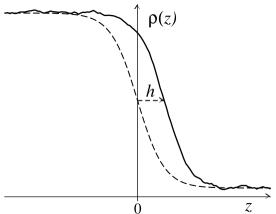
Figure 1: Sketch of the fluctuating density profile as a function of $z$; the height $h\!=\!h(\vec{r}_{\parallel})$ is the distance over which the intrinsic density profile $\rho_{0}(z)$ (dashed line) is shifted.

Adding short wavelength, bulk-like fluctuations to the fluctuating density, the full picture that emerges for $\rho(\vec{r})$ is that schematically depicted in Figure 1. It can be described as:

$$\rho(\vec{r})=\rho_{0}(z)-\rho^{\prime}_{0}(z)\,h(\vec{r}_{\parallel})-\frac{\rho_{1}(z)}{2}\,\Delta h(\vec{r}_{\parallel})+\delta\rho_{b}(\vec{r})$$ (29)

where $\delta\rho_{b}(\vec{r})$ represents the bulk-like fluctuations. We shall consider only small fluctuations so that $<\!\delta\rho_{b}\!>=\!0$ and assume that there are no correlations between height fluctuations and bulk-like fluctuations, $<\!h\,\delta\rho_{b}\!>=\!0$. When we insert the expression for $\rho(\vec{r})$ as given by Eq.(29) into the expression for $S(r_{\parallel})$ in Eq.(23), one finds that

$$S(r_{\parallel})=\,\,S^{ic}_{hh}(r_{\parallel})$$ (30)

$$\hskip 5.0pt+\frac{1}{(\Delta\rho)^{2}}\,\int\limits_{-L}^{L}\!\!dz_{1}\!\int\limits_{-\infty}^{\infty}\!\!\!dz_{12}<\!\delta\rho_{b}(\vec{r}_{1})\,\delta\rho_{b}(\vec{r}_{2})\!>\,.$$

Here we have made a further approximation by replacing the integration over $z_{2}$ from $-L$ to $L$ by an integral over $z_{12}$ from $-\infty$ to $\infty$. The integral over $z_{1}$ that is left gives rise to a term that increases linearly with $L$. That means that the bulk-like contributions to $S(r_{\parallel})$ eventually dominate the height fluctuations when $L$ becomes larger. To study surface fluctuations via $S(r_{\parallel})$ it is therefore important that on the one hand $L$ is sufficiently large in order to make the approximations in, e.g., Eq.(II.2) but on the other hand not so large as to completely dominate the contribution from surface height fluctuations. In the next section we show how these two conditions pan out for the circumstances under which the simulation results are obtained.

A further issue is that the bulk density correlation function $<\!\delta\rho_{b}\,\delta\rho_{b}\!>$ differs in either phase (liquid or vapor). When one then considers the integral over $z_{1}$, it seems appropriate to approximate $<\!\delta\rho_{b}\,\delta\rho_{b}\!>$ by the density correlation function in the bulk liquid region:

$$<\!\delta\rho_{b}(\vec{r}_{1})\,\delta\rho_{b}(\vec{r}_{2})\!>\,=\rho_{\ell}^{2}\,\left[\,g_{\ell}(r)-1\,\right]+\rho_{\ell}\,\delta(\vec{r}_{12})\,,$$ (31)

and introduce an $L$-dependent prefactor ${\cal N}_{L}$ to account for the integral over $z_{1}$. The surface structure factor thus becomes

$$S(q)=S^{ic}_{hh}(q)+{\cal N}_{L}\,S_{b}(q)\,,$$ (32)

with the bulk structure factor $S_{b}(q)$ defined as

$$S_{b}(q)=1+\rho_{\ell}\int\!\!d\vec{r}_{12}\,e^{-i\vec{q}\cdot\vec{r}_{12}}\;\left[\,g_{\ell}(r)-1\,\right]\,.$$ (33)

This approximation may be justified by arguing that close to the critical point there is no distinction between the two bulk correlation functions, whereas far from the critical point the contribution from the bulk vapor can be neglected since $\rho_{v}\!\approx\!0$.

The value for the $L$-dependent prefactor ${\cal N}_{L}$ may be determined from a fit to the limiting behavior of $S(q)$ at $q\rightarrow\!\infty$. For an explicit evaluation of $S_{b}(q)$, we have taken for $g_{\ell}(r)$ the Percus-Yevick solution PY for the hard-sphere correlation function, $g_{\ell}(r)\!=\!g_{\rm hs}^{\rm PY}(r;\rho_{\ell})$.

III Comparison with Monte Carlo simulations

In this section, the surface structure factor in Eq.(32) is compared to results from Monte Carlo simulations by Vink et al. Vink . The system considered consists of a mixture of colloidal particles with diameter $d$ and polymer particles with diameter $2R_{\rm g}$. The colloid-colloid and colloid-polymer interactions are considered to be hard-sphere like, whereas polymer-polymer interactions are taken ideal. The presence of polymer induces a depletion attraction between the colloidal particles which may ultimately lead to phase separation AOVrij ; Gast ; Aarts ; Lekkerkerker92 . The resulting interface of the demixed colloid-polymer system is studied by Vink et al. Vink for a number of polymer concentrations and for a polymer-colloid size ratio parameter $\varepsilon\!\equiv\!1+2R_{\rm g}/d\!=\!$ 1.8.

To study the interfacial fluctuations, Vink et al. introduce the local interface position as Vink :

$$z_{G}(\vec{r}_{\parallel})\equiv\frac{1}{\Delta\rho}\int\limits_{-L}^{L}\!\!dz\left[\,\rho(\vec{r})-\rho_{\rm step}(z)\,\right]\,,$$ (34)

where $\rho(\vec{r})$ can be taken to be either the colloid or polymer density. The integration limits $\pm L$ are inside the bulk regions, but different values for it are systematically considered Vink . One may easily verify that the correlations of the local interface position are exactly described by the surface structure factor defined earlier in Eq.(23)

$$<\!z_{G}(\vec{r}_{1,\parallel})\,z_{G}(\vec{r}_{2,\parallel})\!>\,=\,S(r_{\parallel})\,.$$ (35)

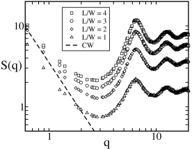
Figure 2: MC results by Vink (Ref. Vink, ) for the surface structure factor (in units of $d^{4}$) versus $q$ (in units of $1/d$) for various values of the integration limit $L/W\!=\!$ 1, 2, 3, 4. The dashed line is the capillary wave model. In this example $\varepsilon\!=\!$ 1.8, $\eta_{p}\!=\!$ 1.0, and the colloidal particles are used to define $z_{G}$.

In Figure 2, typical results for the Fourier transform of the surface structure obtained in the MC simulations of Vink are shown (Figure 13 of ref. Vink, ). In this example the integration limit is varied, $L/W\!=\!$ 1, 2, 3, 4, where $W$ is some measure of the interfacial thickness. One clearly observes that when $L/W$ is too small, the results do not match the classical capillary wave behavior for small $q$ (dashed line), and that the contribution from bulk-like fluctuations at high $q$ increases with $L/W$.

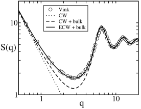
Figure 3: MC results by Vink et al. (Ref. Vink, ) for the surface structure factor (in units of $d^{4}$) versus $q$ (in units of $1/d$). The dotted line is the capillary wave model, the dashed line is the combination of the capillary wave model and the bulk correlation function, and the drawn line is the combination of the extended capillary wave model and the bulk correlation function. In this example $\varepsilon\!=\!$ 1.8, $\eta_{p}\!=\!$ 1.0, $L/W\!=\!$ 3, and the colloidal particles are used to define $z_{G}$.

In Figure 3, we consider the result from Figure 2 for $L/W\!=\!$ 3. For small $q$ the results asymptotically approach the result of the classical capillary wave model (dotted line) with the value of $\sigma$ taken from separate simulations. The dashed line is the combination of the capillary wave model with the bulk correlation function:

$$S(q)=\frac{k_{\rm B}T}{\sigma\,q^{2}}+{\cal N}_{L}\,S_{b}(q)\,.$$ (36)

The value of ${\cal N}_{L}$ is chosen such that it matches the $q\!\rightarrow\!\infty$ limit for $S(q)$ in Figure 3. One finds that Eq.(36) already matches the simulation results quite accurately except at intermediate values of $q$, $qd\!\approx\!1$.

As a next step, we investigate whether the inclusion of a bending rigidity is able to describe the simulation results at these intermediate values:

$$S(q)=\frac{k_{\rm B}T}{\sigma\,q^{2}+k^{ic}\,q^{4}+..}+{\cal N}_{L}\,S_{b}(q)\,.$$ (37)

The bending rigidity describes the leading order correction to the classical capillary wave model in an expansion in $q^{2}$. Its value is therefore obtained from analyzing the behavior of $S(q)$ when $qd\!\apprle\!1$. The fact that the simulation results in Figure 3 are systematically above the capillary wave prediction in this region, indicates that the bending rigidity thus obtained is negative, $k^{ic}\!<\!0$. Unfortunately, a negative bending rigidity prohibits the use of Eq.(37) to fit the simulation results in the entire $q$-range since the denominator becomes zero at a certain value of $q$. It is therefore convenient to rewrite the expansion in $q^{2}$ in Eq.(37) in the following form:

$$S(q)=\frac{k_{\rm B}T}{\sigma\,q^{2}}\,(1-\frac{k^{ic}}{\sigma}\,q^{2}+\ldots)+{\cal N}_{L}\,S_{b}(q)\,,$$ (38)

which is equivalent to Eq.(37) to the order in $q$ considered, but which has the advantage of being well-behaved in the entire $q$-range. Other forms to regulate $S(q)$, that are equivalent to Eq.(37) to the order in $q$ considered, may certainly be formulated. In analogy with a similar treatment of capillary waves by Parry and coworkers Parry08 in the context of wetting transitions, one might suggest that the appearance of a negative bending rigidity indicates the missing of a correlation length that would replace Eq.(38) with an explicit formula valid for all values of $q$, not just to the order in $q$ considered.

The above form for $S(q)$ in Eq.(38), with the bending rigidity used as an adjustable parameter ($k\!=$ - 0.045 $k_{\rm B}T$), is plotted in Figure 3 as the drawn line. Exceptionally good agreement with the Monte Carlo simulations is obtained. In Table 1, we list values of the bending rigidity obtained for a number of polymer volume fractions, $\eta_{p}$. These values are the results of fits of $S(q)$ from Monte Carlo simulations for several system sizes and for several values of $L/W$, with the error estimated from the standard deviation of the various results. For the $L/W\!=\!1$ and $L/W\!=\!2$ curves (see Figure 2), one needs to adjust for the fact that the capillary wave limit is not correctly approached at low $q$. For the results in Figure 2, one ultimately obtains for the bending rigidity $k\!=$ - 0.040, - 0.040, - 0.045, - 0.060 $k_{\rm B}T$, for $L/W\!=\!$ 1, 2, 3, and 4, respectively.

In Table 1, it should be reminded that, rather than the true polymer volume fraction in either phase, $\eta_{p}$ should be interpreted as the polymer volume fraction of a reservoir fixing the polymer chemical potential Lekkerkerker90 . Furthermore, the “liquid” is defined as the phase relatively rich in colloids and the “vapor” as the phase relatively poor in colloids.

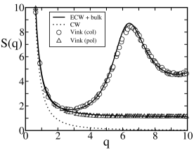
Figure 4: MC results by Vink et al. (Ref. Vink, ) for the surface structure factor (in units of $d^{4}$) versus $q$ (in units of $1/d$) using the colloidal particles (circles) and polymer particles (triangles) to define $z_{G}$. The dotted line is the capillary wave model and the drawn lines are the combination of the extended capillary wave model and the bulk correlation function. In this example $\varepsilon\!=\!$ 1.8, $\eta_{p}\!=\!$ 1.0 and $L/W\!=\!$ 3.

The excellent agreement between Eq.(38) and the MC simulations is even more apparent in Figure 4 where the results in Figure 3 are redrawn on a linear scale. In Figure 4 we also show the simulation results Vink and the corresponding fit using the polymer particles to define the location of the interface. As the polymer-polymer interactions are considered ideal, the bulk structure factor $S_{b}(q)\!=\!1$ in this case.

It is important to note that, effectively, the inclusion of a bending rigidity in the capillary wave model results in the presence of an additive factor in $S(q)$ that is adjusted, see Eq.(38). The determination of the value for $k^{ic}$ from the behavior of $S(q)$ near $q\!=\!0$, therefore requires one to take into account the presence of the bulk-like fluctuations since they also contribute as an additive constant, ${\cal N}_{L}\,S_{b}(0)$, near $q\!=\!0$. This means that even though the MC simulation results of Vink et al. Vink are very accurately described by Eq.(38), the resulting value obtained for $k^{ic}$ sensitively depends on the theoretical expression used for $S_{b}(0)$. Here we have simply approximated the bulk correlation function by the Percus-Yevick hard-sphere expression in the liquid PY , but one could imagine more sophisticated expressions leading to a somewhat different value for $k^{ic}$.

In the next sections we investigate whether the values for the bending rigidity obtained from the simulations (Table 1), can also be described in the context of a molecular theory.

$\eta_{p}$	$\eta_{\ell}$	$\eta_{v}$	$\sigma$	$k$	$\sqrt{-k/\sigma}$
0.9	0.2970	0.0141	0.1532	-0.045 (15)	0.40
1.0	0.3271	0.0062	0.2848	-0.07 (2)	0.50
1.1	0.3485	0.0030	0.4194	-0.10 (3)	0.49
1.2	0.3647	0.0018	0.5555	-0.14 (3)	0.50

Table 1: Listed are the simulation results (Ref. Vink, ) for the polymer volume fraction $\eta_{p}$, liquid and vapor colloidal volume fractions, $\eta_{\ell}$ and $\eta_{v}$, surface tension $\sigma$ (in units of $k_{\rm B}T/d^{2}$), bending rigidity $k$ (in units of $k_{\rm B}T$; in parenthesis the estimated error in the last digit), and $\sqrt{-k/\sigma}$ (in units of $d$).

IV Density functional theory

Our task in this section is straightforward. Using the expression for $\rho(\vec{r})$ given in Eq.(9), we determine $\Delta\Omega$ and the resulting $\sigma(q)$. To achieve this, we need a model for the free energy and define a procedure to determine the density profiles, $\rho_{0}(z)$ and $\rho_{1}(z)$, that are present in the expression for $\rho(\vec{r})$. We choose to perform these tasks in the context of density functional theory (DFT).

In the density functional theory for an inhomogeneous system that we consider Evans ; Henderson ; RW ; Mecke , the free energy is given by the free energy of the reference hard sphere system augmented by an integral, non-local term that considers the attractive part of the interaction potential, $U(r)\!=\!U_{\rm hs}(r)+U_{\rm att}(r)$,

$$\Omega[\rho] = \int\!\!d\vec{r}_{1}\;g_{\rm hs}(\rho)$$

$$+\frac{1}{2}\int\!\!d\vec{r}_{1}\!\int\!\!d\vec{r}_{2}\;U_{\rm att}(r)\,\rho(\vec{r}_{1})\rho(\vec{r}_{2})\,.$$

For explicit calculations, $g_{\rm hs}(\rho)$ is taken to be of the Carnahan-Starling form CS :

$$g_{\rm hs}(\rho)=k_{\rm B}T\,\rho\,\ln(\rho)+k_{\rm B}T\,\rho\,\frac{(4\eta-3\eta^{2})}{(1-\eta)^{2}}-\mu\rho\,,$$ (40)

where $\eta\!\equiv\!(\pi/6)\,\rho\,d^{3}$. In the uniform bulk region, the free energy equals

$$\frac{\Omega(\rho)}{V}\equiv g(\rho)=g_{\rm hs}(\rho)-a\rho^{2}\,,$$ (41)

with the van der Waals parameter $a$ given by RW

$$a\equiv-\frac{1}{2}\,\int\!\!d\vec{r}_{12}\;U_{\rm att}(r)\,.$$ (42)

The integration over $\vec{r}_{12}$ is restricted to the region $r\!>\!d$. This is not explicitly indicated; instead, we adhere to the convention that the attractive part of the interaction potential $U_{\rm att}(r)\!=\!0$ when $r\!<\!d$. The chemical potential $\mu$ is fixed by the condition of two-phase coexistence, $\mu\!=\!\mu_{\rm coex}$, which implies that $\mu_{\rm coex}$, $\rho_{v}$, and $\rho_{\ell}$ are determined from the set of equations: $g^{\prime}(\rho_{v})\!=\!0$, $g^{\prime}(\rho_{\ell})\!=\!0$, and $g(\rho_{v})\!=\!g(\rho_{\ell})\!=\!-p$.

To determine the change in free energy due to density fluctuations, we insert the expression for $\rho(\vec{r})$ given by Eq.(9) into the expression for $\Omega$ in Eq.(IV). One then finds for $\Delta\Omega\!=\!\Omega-\sigma A$

$$\Delta\Omega=\frac{1}{8}\int\!\!d\vec{r}_{1}\;\Big{\{}g_{\rm hs}^{\prime\prime}(\rho_{0})\rho_{1}(z_{1})^{2}\left[\Delta h(\vec{r}_{1,\parallel})\right]^{2}$$

$$+\frac{1}{8}\int\!\!d\vec{r}_{1}\int\!\!d\vec{r}_{12}\;U_{\rm att}(r)\times$$

$$\left\{-2\,\rho_{0}^{\prime}(z_{1})\rho_{0}^{\prime}(z_{2})\left[h(\vec{r}_{2,\parallel})-h(\vec{r}_{1,\parallel})\right]^{2}\right.$$

$$\hskip 7.0pt+4\,\rho_{1}(z_{1})\rho_{0}^{\prime}(z_{2})\,\Delta h(\vec{r}_{1,\parallel})\left[h(\vec{r}_{2,\parallel})-h(\vec{r}_{1,\parallel})\right]$$

$$\hskip 7.0pt+\rho_{1}(z_{1})\rho_{1}(z_{2})\,\Delta h(\vec{r}_{1,\parallel})\Delta h(\vec{r}_{2,\parallel})\Big{\}}\,.$$ (43)

Even though the derivation is somewhat different, this expression equals that given by Mecke and Dietrich Mecke apart from a gravity term that was included in their expression. To cast $\Delta\Omega$ in the form of Eq.(11), we take the Fourier Transform. One then finds for $\sigma(q)$ Mecke

$$\sigma(q) = \int\limits_{-\infty}^{\infty}\!\!\!dz_{1}\!\int\limits_{-\infty}^{\infty}\!\!\!dz_{12}\;\left[\frac{\omega(q,z_{12})-\omega_{0}(z_{12})}{q^{2}}\right]$$ (44)

$$\!\!\times\left[\,\rho_{0}^{\prime}(z_{1})\rho_{0}^{\prime}(z_{2})-q^{2}\,\rho_{1}(z_{1})\rho_{0}^{\prime}(z_{2})\,\right]$$

$$\!\!+\frac{q^{2}}{4}\int\limits_{-\infty}^{\infty}\!\!\!dz_{1}\!\!\int\limits_{-\infty}^{\infty}\!\!\!dz_{12}\;\omega(q,z_{12})\,\rho_{1}(z_{1})\rho_{1}(z_{2})$$

$$\!\!+\frac{q^{2}}{4}\int\limits_{-\infty}^{\infty}\!\!\!dz_{1}\;g_{\rm hs}^{\prime\prime}(\rho_{0})\rho_{1}(z_{1})^{2}\,.$$

Here we have defined the (parallel) Fourier Transform of the interaction potential

$$\omega(q,z_{12}) \equiv \int\!\!d\vec{r}_{\parallel}\,e^{-i\vec{q}\cdot\vec{r}_{\parallel}}\,U_{\rm att}(r)$$

$$= 2\pi\!\int\limits_{0}^{\infty}\!\!dr_{\parallel}\,r_{\parallel}\,J_{0}(qr_{\parallel})\,U_{\rm att}(r)\,.$$

As a first step, we determine the leading contribution to $\sigma(q)$ given by the surface tension of the planar interface, $\sigma\!=\!\sigma(q\!=\!0)$. Then, one needs to consider the two leading contributions in the expansion of $\omega(q,z_{12})$ in $q^{2}$:

$$\omega(q,z_{12})=\omega_{0}(z_{12})+\omega_{2}(z_{12}){q^{2}}+\ldots\,,$$ (46)

where

$$\omega_{0}(z_{12}) \equiv \int\!\!d\vec{r}_{\parallel}\;U_{\rm att}(r)\,,$$

$$\omega_{2}(z_{12}) \equiv -\frac{1}{4}\int\!\!d\vec{r}_{\parallel}\;r_{\parallel}^{2}\,U_{\rm att}(r)\,.$$ (47)

The surface tension thus becomes

$$\sigma=\int\limits_{-\infty}^{\infty}\!\!\!dz_{1}\int\limits_{-\infty}^{\infty}\!\!\!dz_{12}\;\omega_{2}(z_{12})\,\rho_{0}^{\prime}(z_{1})\rho_{0}^{\prime}(z_{2})\,.$$ (48)

The (planar) density profile $\rho_{0}(z)$, featured in the above expression for $\sigma$, is determined from minimizing the free energy functional $\Omega[\rho]$ in Eq.(IV) in planar symmetry. The Euler-Lagrange equation that minimizes $\Omega[\rho]$ is then given by:

$$g^{\prime}_{\rm hs}(\rho_{0}) = -\int\!\!d\vec{r}_{12}\;U_{\rm att}(r)\,\rho_{0}(z_{2})$$ (49)

$$= -\int\limits_{-\infty}^{\infty}\!\!\!dz_{12}\;\omega_{0}(z_{12})\,\rho_{0}(z_{2})\,,$$

which can be solved explicitly to obtain $\rho_{0}(z)$ and thus $\sigma$.

The evaluation of further contributions to $\sigma(q)$ requires one to determine the density profile $\rho_{1}(z)$. Just like $\rho_{0}(z)$, one would like to determine the density profile $\rho_{1}(z)$ from a minimization procedure. One then has to determine the energetically most favorable density profile for a given curvature of the surface Parry94 . This turns out to be not so straightforward, since one then has to specify in what way the curvature is set to its given value. Several approaches have been suggested, which we shall now discuss.

• Mecke and Dietrich approach. In this approach a certain form for $\rho_{1}(z)$ is directly hypothesized Mecke :

  $$\rho^{\rm MD}_{1}(z)=-\frac{C_{\rm H}}{2\pi}\,\Delta\rho\,\xi\,f_{\rm H}(z/\xi)\,,$$ (50)

  with $\xi$ the bulk correlation length and $f_{\rm H}(x)\!\equiv\!x\sinh(x/2)/\cosh^{2}(x/2)$. The coefficient $C_{\rm H}$ in this expression can be used as a fit parameter. This practical approach is certainly legitimate, but one would like to also be able to formulate a molecular basis for this expression.

• Equilibrium approach. Rather than the surface being curved by surface fluctuations, in this approach the interface is curved by changing the value of the chemical potential to a value off-coexistence. One then considers the density profile of a spherically or cylindrically shaped liquid droplet in metastable equilibrium with a bulk vapor Blokhuis93 ; Gompper . This approach is equivalent to adding an external field to the free energy

  $$\Omega^{\prime}[\rho] = \Omega[\rho]+\int\!\!d\vec{r}\;V_{\rm ext}(\vec{r})\,\rho(\vec{r})$$ (51)

  $$= \Omega[\rho]-\int\!\!d\vec{r}\;\Delta\mu\,\rho(\vec{r})\,,$$

  where $\Delta\mu\!=\!\mu-\mu_{\rm coex}$. The downside of the equilibrium approach is that the external field $V_{\rm ext}(\vec{r})\!=\!-\Delta\mu$ is uniform throughout the system and thus also affects the bulk densities far from the interfacial region. This seems inappropriate for the description of the density fluctuations considered here since we have that $\mu\!=\!\mu_{\rm coex}$ and the bulk densities are unaltered by the curvature of the surface fluctuations.

• Local external field. In this approach, one again adds to the free energy an external field, but, to ensure that the bulk regions are unaffected, one assumes that it is peaked infinitely sharply at $z\!=\!0$ Parry94 ; Blokhuis99 :

  $$V_{\rm ext}(\vec{r})=\lambda\,\delta(z)\,\Delta h(\vec{r}_{\parallel})\,.$$ (52)

  In this case, the external field only acts as a Lagrange multiplier in the minimization procedure to ensure that the curvature $\Delta h(\vec{r}_{\parallel})$ is set to a certain value; it is not included in the expression for the free energy. The downside of this method is that the resulting density profile $\rho_{1}(z)$ has a discontinuous first derivative at $z\!=\!0$, which is, from a physical point of view, not so appealing FJ . Furthermore, the discontinuous nature of $\rho_{1}(z)$ prohibits an analytical simplification using a gradient expansion.

In the present approach, we suggest to add an external field acting as a Lagrange multiplier that is unequal to zero only in the interfacial region (the bulk densities are unaffected), but which is not infinitely sharp-peaked. It seems natural to choose a peak-width of the order of the thickness of the interfacial region. It thus seems convenient to choose $V_{\rm ext}(\vec{r})\!\propto\!\rho^{\prime}_{0}(z)$:

$$V_{\rm ext}(\vec{r})=\lambda\,\rho^{\prime}_{0}(z)\,\Delta h(\vec{r}_{\parallel})\,.$$ (53)

This choice for $V_{\rm ext}(\vec{r})$ constitutes our fundamental ‘Ansatz’ for the determination of $\rho_{1}(z)$. The Lagrange multiplier $\lambda$ is not a free parameter but set by the imposed curvature, as demonstrated below.

The addition of an external field to the free energy results in the following Euler-Lagrange equation:

$$g^{\prime}_{\rm hs}(\rho)=-\int\!\!d\vec{r}_{12}\;U_{\rm att}(r)\,\rho(\vec{r}_{2})-V_{\rm ext}(\vec{r})\,.$$ (54)

Using the external field given in Eq.(53), we insert the fluctuating density given by Eq.(9) into the above Euler-Lagrange equation. In order for the resulting equation to hold independently of the value of $h(\vec{r}_{\parallel})$ or $\Delta h(\vec{r}_{\parallel})$, one finds, besides Eq.(49), the following equation to determine $\rho_{1}(z)$:

$$g^{\prime\prime}_{\rm hs}(\rho_{0})\rho_{1}(z_{1})=-\int\limits_{-\infty}^{\infty}\!\!\!dz_{12}\;\omega_{0}(z_{12})\,\rho_{1}(z_{2})$$

$$+2\int\limits_{-\infty}^{\infty}\!\!\!dz_{12}\;\omega_{2}(z_{12})\,\rho^{\prime}_{0}(z_{2})+2\,\lambda\,\rho^{\prime}_{0}(z_{1})\,.$$ (55)

The value of the Lagrange multiplier can be determined by multiplying both sides of the above expression by $\rho^{\prime}_{0}(z_{1})$ and integrating over $z_{1}$:

$$\lambda=-\sigma/\left[\int\!\!dz\;[\rho_{0}^{\prime}(z)]^{2}\right]\,.$$ (56)

One may now verify that if $\rho_{1}(z)$ is a particular solution of Eq.(IV) that then also $\rho_{1}(z)+\alpha\,\rho^{\prime}_{0}(z)$ is a solution on account of Eq.(49).

It is convenient to use the Euler-Lagrange equation in Eq.(IV) to remove the explicit appearance of $g^{\prime\prime}_{\rm hs}(\rho_{0})$ in the expression for $\sigma(q)$ in Eq.(44). The resulting $\sigma(q)$ is written as the sum of a term that depends only on the density profile $\rho_{0}(z)$ and one term that also depends on the density profile $\rho_{1}(z)$

$$\sigma(q)=\sigma_{0}(q)+k_{1}\,q^{2}+{\cal O}(q^{4})\,,$$ (57)

with

$$\sigma_{0}(q) \equiv \int\limits_{-\infty}^{\infty}\!\!\!dz_{1}\!\int\limits_{-\infty}^{\infty}\!\!\!dz_{12}\left[\frac{\omega(q,z_{12})-\omega_{0}(z_{12})}{q^{2}}\right]$$

$$\hskip 60.0pt\times\,\rho_{0}^{\prime}(z_{1})\rho_{0}^{\prime}(z_{2})\,,$$

$$k_{1} \equiv -\frac{1}{2}\int\limits_{-\infty}^{\infty}\!\!\!dz_{1}\!\int\limits_{-\infty}^{\infty}\!\!\!dz_{12}\;\omega_{2}(z_{12})\,\rho_{1}(z_{1})\rho_{0}^{\prime}(z_{2})$$ (58)

$$+\frac{\lambda}{2}\int\limits_{-\infty}^{\infty}\!\!\!dz_{1}\;\rho_{1}(z_{1})\rho_{0}^{\prime}(z_{1})\,.$$

With the above expression for $k_{1}$ it is now also possible to verify that when the density profile $\rho_{1}(z)$ is shifted by a factor $\alpha\rho^{\prime}_{0}(z)$, that the resulting effect on the bending parameters is that given by Eq.(II.2).

The procedure to determine $\sigma(q)$, and therefore $\sigma$, $k$, $k_{s}$, and $\ell_{k}$, is now as follows: assuming a certain form for the attractive part of the interaction potential, $\rho_{0}(z)$ is obtained from solving Eq.(49), which is then inserted into Eq.(IV) to solve for $\rho_{1}(z)$ explicitly. The two density profiles thus obtained are inserted into Eq.(IV) to yield $\sigma_{0}(q)$ and $k_{1}$. This procedure is carried out in the next two sections considering short-ranged forces and long-ranged forces ($U(r)\!\propto\!1/r^{6}$). In general the density profiles $\rho_{0}(z)$ and $\rho_{1}(z)$ need to be determined numerically. We shall, however, also provide an approximation scheme, based on the gradient expansion, that is exact near the critical point, but which also gives an excellent approximation far from it.

IV.1 Gradient expansion

The gradient approximation RW is based on the assumption that the spatial variation of the density profile is small, i.e.

$$\rho(z_{2})=\rho(z_{1})+z_{12}\,\rho^{\prime}(z_{1})+\frac{z_{12}^{2}}{2}\,\rho^{\prime\prime}(z_{1})+\ldots$$ (59)

In the gradient expansion, the Euler-Lagrange equation in Eq.(49) for $\rho_{0}(z)$ reduces to

$$g^{\prime}(\rho_{0})=2m\,\rho^{\prime\prime}_{0}(z)\,,$$ (60)

where $m$ is the van der Waals squared-gradient coefficient RW

$$m \equiv -\frac{1}{12}\,\int\!\!d\vec{r}_{12}\;r^{2}\,U_{\rm att}(r)$$

$$= \frac{1}{2}\int\limits_{-\infty}^{\infty}\!\!\!dz_{12}\;\omega_{2}(z_{12})=\frac{1}{4}\int\limits_{-\infty}^{\infty}\!\!\!dz_{12}\;z_{12}^{2}\,\omega_{0}(z_{12})\,.$$

In the gradient expansion, the Euler-Lagrange equation in Eq.(IV) for $\rho_{1}(z)$ reduces to

$$m\,\frac{\rho_{0}^{\prime\prime\prime}(z_{1})}{\rho_{0}^{\prime}(z_{1})}\rho_{1}(z_{1})=m\,\rho_{1}^{\prime\prime}(z_{1})$$ (62)

$$\hskip 40.0pt+\int\limits_{-\infty}^{\infty}\!\!\!dz_{12}\;\omega_{2}(z_{12})\,\rho_{0}^{\prime}(z_{2})+\lambda\,\rho^{\prime}_{0}(z_{1})\,,$$

where we have used Eq.(60) to replace $g^{\prime\prime}_{\rm hs}(\rho_{0})$.

First, we consider the determination of the density profile $\rho_{0}(z)$. The gradient expansion becomes exact near the critical point where $g(\rho)$ takes on the usual double-well form

$$g(\rho)+p=\frac{m}{(\Delta\rho)^{2}\,\xi^{2}}\,(\rho-\rho_{\ell})^{2}\,(\rho-\rho_{v})^{2}\,.$$ (63)

Using this form for $g(\rho)$, the solution of the Euler-Lagrange equation in Eq.(60) gives the usual $\tanh$-form for $\rho_{0}(z)$ RW :

$$\rho_{0}(z)=\frac{1}{2}(\rho_{\ell}+\rho_{v})-\frac{\Delta\rho}{2}\,\tanh(z/2\xi)\,,$$ (64)

with the bulk correlation length $\xi$ a measure of the interfacial thickness.

Even though the $\tanh$-form for the density profile $\rho_{0}(z)$ is derived assuming proximity to the critical point, it turns out that it also provides a good approximation away from it when one determines the value of $\xi$ by fitting the surface tension to its form near the critical point. In the squared-gradient approximation, Eq.(48) reduces to the familiar expression RW

$$\sigma = 2\,m\int\limits_{-\infty}^{\infty}\!\!\!dz\;\rho_{0}^{\prime}(z)^{2}$$ (65)

$$= 2\,\sqrt{m}\int\limits_{\rho_{v}}^{\rho_{\ell}}\!\!d\rho\;\sqrt{g(\rho)+p}\,.$$

On the one hand, the surface tension can be determined from the above approximation using the full form for $g(\rho)$ given in Eqs.(40) and (41):

$$\sigma = 2\,\sqrt{m}\int\limits_{\rho_{v}}^{\rho_{\ell}}\!\!d\rho\;\bigl{[}k_{\rm B}T\,\rho\,\ln(\rho)$$

$$+k_{\rm B}T\,\rho\,\frac{(4\eta-3\eta^{2})}{(1-\eta)^{2}}-\mu_{\rm coex}\rho-a\rho^{2}+p\bigr{]}^{\!\frac{1}{2}}\,.$$

On the other hand, near the critical point $g(\rho)$ takes on the double-well form in Eq.(63) and $\sigma$ is calculated as

$$\sigma=\frac{m\,(\Delta\rho)^{2}}{3\,\xi}\,.$$ (67)

Now, we define the value of $\xi$ such that the two expressions for the surface tension in Eqs.(IV.1) and (67) are equal. This gives for $\xi$:

$$\xi\equiv\frac{m\,(\Delta\rho)^{2}}{3\,\sigma}\,,$$ (68)

with $\sigma$ given by Eq.(IV.1).

Next, we turn to the evaluation of $\rho_{1}(z)$ from Eq.(62). This requires one to make a distinction between short-ranged forces and long-ranged forces.

V DFT: short-ranged interactions

Although the analysis below is quite generally valid for all short-ranged interaction potentials, whenever we show explicit results, we consider for $U_{\rm att}(r)$ the Asakura-Oosawa-Vrij depletion interaction potential $U_{\rm dep}(r)$ as an example AOVrij :

$$U_{\rm dep}(r)=\frac{-k_{\rm B}T\,\eta_{p}}{2\,(\varepsilon-1)^{3}}\left[\,2\,\varepsilon^{3}-3\,\varepsilon^{2}\left(\frac{r}{d}\right)+\left(\frac{r}{d}\right)^{\!3}\,\right]$$ (69)

where the intermolecular distance is in the range $1\!<\!r/d\!<\!\varepsilon$. Interaction parameters based on the depletion potential are listed in the Appendix. The strength of the depletion interaction potential as determined by the polymer volume fraction $\eta_{p}$ determines the location in the phase diagram Gast ; Lekkerkerker90 ; for comparison with other results, it is, however, more convenient to use the colloidal density difference $\Delta\eta\!\equiv\!\eta_{\ell}-\eta_{v}$ as thermodynamic variable Kuipers .

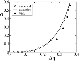
Figure 5: Surface tension in units of $k_{\rm B}T/d^{2}$ versus the volume fraction difference, $\Delta\eta$. In this example $\varepsilon\!=\!1.8$; symbols are numerical results, the drawn line is the gradient expansion approximation, filled symbols are results from the MC simulations by Vink et al. (Ref. Vink, ).

In Figure 5, the surface tension is shown as a function of $\Delta\eta$. The open circles are obtained from numerically solving the Euler-Lagrange equation in Eq.(49) for $\rho_{0}(z)$ and inserting the result into Eq.(48). The drawn line is the gradient expansion approximation for $\sigma$ in Eq.(IV.1). Also shown are results from the MC simulations by Vink et al. Vink . The gradient expansion gives a very good approximation to the numerical results and is in good agreement with the simulations.

For short-ranged forces the expansion in $q^{2}$ of the expression for $\omega(q,z_{12})$ as defined by Eq.(IV) can be continued to ${\cal O}(q^{4})$:

$$\omega(q,z_{12})=\omega_{0}(z_{12})+\omega_{2}(z_{12})\,q^{2}+\omega_{4}(z_{12})\,q^{4}+\ldots$$ (70)

where

$$\omega_{4}(z_{12})\equiv\frac{1}{64}\int\!\!d\vec{r}_{\parallel}\;r_{\parallel}^{4}\,U_{\rm att}(r)\,.$$ (71)

With this expansion, $\sigma(q)$ in Eq.(IV) can now be written in the form of Eq.(13)

$$\sigma(q) = \sigma+k\,q^{2}+{\cal O}(q^{4})$$ (72)

$$= \sigma+k_{0}\,q^{2}+k_{1}\,q^{2}+{\cal O}(q^{4})\,,$$

with the bending rigidity $k\!=\!k_{0}+k_{1}$ and

$$k_{0} = \int\limits_{-\infty}^{\infty}\!\!\!dz_{1}\!\int\limits_{-\infty}^{\infty}\!\!\!dz_{12}\;\omega_{4}(z_{12})\,\rho_{0}^{\prime}(z_{1})\rho_{0}^{\prime}(z_{2})\,,$$

$$k_{1} = -\frac{1}{2}\int\limits_{-\infty}^{\infty}\!\!\!dz_{1}\!\int\limits_{-\infty}^{\infty}\!\!\!dz_{12}\;\omega_{2}(z_{12})\,\rho_{1}(z_{1})\rho_{0}^{\prime}(z_{2})$$ (73)

$$+\frac{\lambda}{2}\int\limits_{-\infty}^{\infty}\!\!\!dz_{1}\;\rho_{1}(z_{1})\rho_{0}^{\prime}(z_{1})\,.$$

Next, we proceed to evaluate these expressions in the gradient expansion.

V.1 Gradient expansion for short-ranged forces

In the gradient expansion, $k_{0}$ and $k_{1}$ in Eq.(V) reduce to:

$$k_{0} = -\frac{B}{2}\int\limits_{-\infty}^{\infty}\!\!\!dz\;\rho_{0}^{\prime}(z)^{2}\,,$$

$$k_{1} = -2\,m\int\limits_{-\infty}^{\infty}\!\!\!dz\;\rho_{1}(z)\,\rho_{0}^{\prime}(z)\,,$$ (74)

where we have used the fact that to leading order in the gradient expansion $\lambda\!\approx\!-2m$, and where we have defined Varea

$$B \equiv -\frac{1}{60}\,\int\!\!d\vec{r}_{12}\;r^{4}\,U_{\rm att}(r)$$

$$= -2\!\int\limits_{-\infty}^{\infty}\!\!\!dz_{12}\;\omega_{4}(z_{12})=\frac{1}{2}\!\int\limits_{-\infty}^{\infty}\!\!\!dz_{12}\;z_{12}^{2}\,\omega_{2}(z_{12})\,.$$

Inserting the $\tanh$-form for $\rho_{0}(z)$ into Eq.(V.1), one directly obtains for $k_{0}$

$$k_{0}=-\frac{B\,(\Delta\rho)^{2}}{12\,\xi}=-\frac{B\,\sigma}{4\,m}\,,$$ (76)

where we have used the expression for $\xi$ in Eq.(68) to rewrite $k_{0}$ as the latter expression.

To evaluate $k_{1}$ in Eq.(V.1), we need to determine $\rho_{1}(z)$ from the Euler-Lagrange equation in Eq.(62). For short-ranged forces, Eq.(62) reduces to

$$m\,\frac{\rho_{0}^{\prime\prime\prime}(z)}{\rho_{0}^{\prime}(z)}\rho_{1}(z)=m\,\rho_{1}^{\prime\prime}(z)+B\,\rho^{\prime\prime\prime}_{0}(z)+\beta\,B\,\rho^{\prime}_{0}(z)\,,$$ (77)

where we have defined

$$\beta\equiv\frac{\int\!dz\;\rho_{0}^{\prime\prime}(z)^{2}}{\int\!dz\;\rho_{0}^{\prime}(z)^{2}}\,.$$ (78)

Using the $\tanh$-profile for $\rho_{0}(z)$ in Eq.(64), one has $\beta\!=\!1/(5\xi^{2})$ and finds for $\rho_{1}(z)$ from solving the differential equation in Eq.(77):

$$\rho^{cc}_{1}(z)=-\frac{3\,B}{10\,m}\frac{\Delta\rho}{\xi}\,\frac{\ln(\cosh(z/2\xi))}{\cosh^{2}(z/2\xi)}\,.$$ (79)

The above profile corresponds to that obtained using the crossing constraint. The profile corresponding to the integral constraint follows from $\rho^{ic}_{1}\!=\!\rho^{cc}_{1}+\alpha\,\rho^{\prime}_{0}$ (Eq.(20)), with $\alpha$ determined by Eq.(21). This gives

$$\!\!\!\rho^{ic}_{1}(z)=\frac{3\,B}{10\,m}\frac{\Delta\rho}{\xi}\,\frac{\left[\,1-\ln(2\,\cosh(z/2\xi))\,\right]}{\cosh^{2}(z/2\xi)}\,.$$ (80)

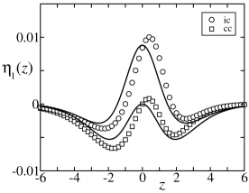
Figure 6: Curvature correction to the volume fraction profile $\eta_{1}(z)$ as a function of $z$ (in units of $d$) using the integral constraint (circles) and crossing constraint (squares). In this example $\Delta\eta\!=\!$ 0.25, $\varepsilon\!=\!1.8$; symbols are numerical results, the drawn lines are the analytical profiles from the gradient expansion.

In Figure 6, typical volume fraction profiles $\eta_{1}(z)\!=\!(\pi/6)\,d^{3}\,\rho_{1}(z)$ are shown for the crossing constraint and the integral constraint. The symbols are the profiles obtained from numerically solving the Euler-Lagrange equation in Eq.(IV), whereas the drawn lines are the approximate profiles in Eqs.(79) and (80) obtained from the gradient expansion.

Inserting the density profiles $\rho^{ic}_{1}(z)$ and $\rho^{cc}_{1}(z)$ into the expression for $k_{1}$ in Eq.(V.1), one obtains

$$k_{1}^{cc} = -\frac{B\,(\Delta\rho)^{2}}{\xi}\,\left[\frac{1}{3}-\frac{2}{5}\,\ln(2)\right]$$

$$= -\frac{B\,\sigma}{m}\,\left[1-\frac{6}{5}\,\ln(2)\right]\,,$$

$$k_{1}^{ic} = \frac{B\,(\Delta\rho)^{2}}{15\,\xi}=\frac{B\,\sigma}{5\,m}\,.$$ (81)

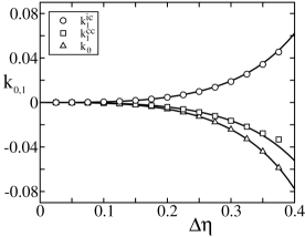
Figure 7: Contributions to the bending rigidity $k_{0}$ and $k_{1}$ in units of $k_{\rm B}T$ versus the volume fraction difference, $\Delta\eta$. In this example $\varepsilon\!=\!1.8$; symbols are numerical results, the drawn lines are the gradient expansion approximation.

In Figure 7, $k_{0}$, $k_{1}^{ic}$ and $k_{1}^{cc}$ are shown as a function of $\Delta\eta$. The open symbols are obtained from numerically solving Eqs.(49) and (IV) to obtain $\rho_{0}(z)$ and $\rho_{1}(z)$ and inserting the result into Eq.(V). The drawn lines are the gradient expansion approximation for $k_{0}$ in Eq.(76) and $k_{1}$ in Eq.(V.1). Adding the results for $k_{1}$ in Eq.(V.1) to $k_{0}$ in Eq.(76), one obtains for the bending rigidities

$$k^{cc} = -\frac{B\,(\Delta\rho)^{2}}{\xi}\,\left[\frac{5}{12}-\frac{2}{5}\,\ln(2)\right]$$

$$= -\frac{B\,\sigma}{m}\,\left[\frac{5}{4}-\frac{6}{5}\,\ln(2)\right]\,,$$

$$k^{ic} = -\frac{B\,(\Delta\rho)^{2}}{60\,\xi}=-\frac{B\,\sigma}{20\,m}\,.$$ (82)

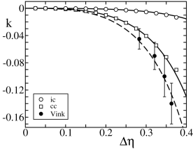
Figure 8: Bending rigidity in units of $k_{\rm B}T$ versus the volume fraction difference, $\Delta\eta$, using the integral constraint (circles) and crossing constraint (squares). In this example $\varepsilon\!=\!1.8$; open symbols are numerical results, the drawn lines are the gradient expansion approximation, filled circles are the MC results by Vink et al. (Ref. Vink, ); the dashed line is the fit $\sqrt{-k/\sigma}\approx$ 0.47 $d$.

In Figure 8, the bending rigidity is shown as a function of $\Delta\eta$. The open symbols are the numerical results. The drawn lines are the gradient expansion approximations in Eq.(V.1), $\sqrt{-k^{cc}/\sigma}\approx$ 0.378 $d$ and $\sqrt{-k^{ic}/\sigma}\approx$ 0.131 $d$.

The resulting values for both bending rigidities, $k^{cc}$ and $k^{ic}$, are negative in line with the simulation results of Vink (filled circles). However, the value of $k^{ic}$, which is the relevant value when we compare with the simulations, is significantly less negative. As stressed earlier, the bending rigidity depends on the constraint used to define the height profile $h(\vec{r}_{\parallel})$ through the contribution to $k$ coming from $k_{1}$. We demonstrated that in the crossing constraint $k^{cc}_{1}$ is negative whereas in the integral constraint $k^{ic}_{1}$ is positive. One could very well imagine that a different constraint used to determine the height profile $h(\vec{r}_{\parallel})$ might lead to a bending rigidity that is positive Tarazona . For the integral constraint the two contributions to $k$ from $k_{0}$ and $k^{ic}_{1}$ nearly cancel leading to a value for $k^{ic}$ which is barely negative. Unfortunately, this makes the value of $k^{ic}$ sensitively dependent on the precise model used to determine $\rho_{1}(z)$.

An important point concerns the scaling behavior of the bending rigidity. The expressions in Eq.(V.1) indicate that the bending rigidity vanishes near the critical point with the same exponent as the surface tension, i.e.

$$k\propto\frac{B\,\sigma}{m}\,\propto\,\sigma\,d^{2}\,.$$ (83)

Note that for the depletion potential, the ratio $B/m$ only depends on the size ratio parameter $\varepsilon$ ($B/m\approx$ 0.342 $d^{2}$ for $\varepsilon\!=\!$ 1.8) but is independent of $\eta_{p}$ (or $\Delta\eta$), see the Appendix. Both contributions to the bending rigidity, $k_{0}$ and $k_{1}$, show the above scaling behavior and both should therefore be taken into account.

The scaling result in Eq.(83) should be contrasted with the usual assumption that $k\!\propto\!\sigma\,\xi^{2}$, i.e. the bending rigidity approaches a finite, non-zero limit at the critical point. This scaling behavior is, for instance, obtained for the bending rigidity $k_{\rm eq}$ determined from analysing the surface tension of a spherically or cylindrically shaped liquid droplet in metastable equilibrium with a bulk vapor Blokhuis93 ; Gompper . In the gradient expansion, one has Blokhuis93 :

$$k_{\rm eq}=-\frac{1}{9}(\pi^{2}-3)\,m\,(\Delta\rho)^{2}\,\xi\,.$$ (84)

It is perhaps important to discuss more broadly this result in the context of previous work on the virial approach Blokhuis92 to the bending rigidity (and other curvature parameters). The virial expression for the bending rigidity is generally valid, but it is important to realise that it features the way in which the pair density depends on curvature Blokhuis92 . When a mean-field, squared-gradient approximation is subsequently made Blokhuis93 , this translates into the expression for the bending rigidity to depend on the way in which the density depends on curvature, i.e. it features the profile $\rho_{1}(z)$. Therefore, even though the expressions for the bending rigidity in the equilibrium approach and the fluctuating interface approach are the same, they might lead to different values (and scaling behavior) of the bending rigidity due to the fact that the density profiles $\rho_{1}(z)$ are different in these two cases.

It is interesting to also compare with the approach by Mecke and Dietrich Mecke . Even though the goal in ref. Mecke, is to consider long-ranged forces, one may use the expression in Eq.(50) for $\rho^{\rm MD}_{1}(z)$ inserted into Eq.(IV) to determine the leading correction to $\sigma(q)$ also for short-ranged forces. The gradient expansion then gives:

$$k_{\rm MD}=-\left[\,\frac{C_{\rm H}}{6}-\frac{C_{\rm H}^{2}}{24\,\pi^{2}}\,(\pi^{2}+16)\,\right]m\,(\Delta\rho)^{2}\,\xi\,.$$ (85)

The prefactor is negative (as long as $0\!<\!C_{\rm H}\!<\!1.526$) in line with the results obtained here. Again, the scaling behavior – equal to that of $k_{\rm eq}$ – is essentially different than our prediction in Eq.(83).

Finally, we like to mention an expression for the bending rigidity that is derived from the generally valid virial expression Blokhuis92 , in which the assumption is made that the width of the interfacial profile is much smaller than the molecular diameter $d\!\gg\!\xi$ Blokhuis92 ; Napiorkowski . The implication is that $\rho_{0}(z)\!=\!\rho_{\rm step}(z)$, the sharp-profile approximation, and $\rho_{1}(z)\!=\!0$. The sharp-profile expressions for the surface tension (also known as the Fowler formula Fowler ) and bending rigidity are Fowler ; Blokhuis92 ; Blokhuis99 :

$$\sigma_{\rm sp} = \frac{(\Delta\rho)^{2}}{32}\,\int\!\!d\vec{r}_{12}\;r^{2}\,U^{\prime}(r)\,g_{\ell}(r)\,,$$ (86)

$$k_{\rm sp} = -\frac{(\Delta\rho)^{2}}{768}\,\int\!\!d\vec{r}_{12}\;r^{4}\,U^{\prime}(r)\,g_{\ell}(r)\,,$$

where $U(r)$ is the full interaction potential. Since $\rho_{1}(z)\!=\!0$, the expression for $k_{\rm sp}$ is independent on the constraint used to determine $\rho_{1}(z)$.

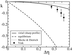
Figure 9: Bending rigidity in units of $k_{\rm B}T$ versus the volume fraction difference, $\Delta\eta$. In this example $\varepsilon\!=\!1.8$; filled circles are the MC results by Vink et al. (Ref. Vink, ), the drawn line is the virial expression with the sharp-profile approximation, the dashed line is the equilibrium result, and the dotted line is the Mecke and Dietrich result (Ref. Mecke, ) with $C_{\rm H}\!=\!1/4$.

In Figure 9, the different models for the bending rigidity are compared to the simulation results of Vink et al. Vink . For the evaluation of $k_{\rm sp}$ we have taken $g_{\ell}(r)\!=\!g_{\rm hs}^{\rm PY}(r;\eta_{\ell})$.

VI DFT: long-ranged interactions

Here we examine the case that the expansion of $\omega(q,z_{12})$ in $q^{2}$ cannot be continued to ${\cal O}(q^{4})$. This is the case when the interaction potential falls of as $1/r^{n}$ at large distances, with $n\!\leq\!6$. In particular, we shall assume the asymptotic behavior of $U_{\rm att}(r)$ to be given by

$$U_{\rm att}(r)=-A/r^{6}\hskip 20.0pt{\rm when}\hskip 10.0ptr\gg d\,.$$ (87)

The analysis below only assumes that the asymptotic behavior of $U_{\rm att}(r)$ is given by the above expression. However, when we show explicit results, we consider the above form for $U_{\rm att}(r)$ extended to the whole range $1\!<\!r/d\!<\!\infty$ (see also the Appendix).

With the asymptotic behavior of $U_{\rm att}(r)$ given by Eq.(87), the expansion of $\omega(q,z_{12})$ in $q^{2}$ takes on the form:

$$\omega(q,z_{12}) = \omega_{0}(z_{12})+\omega_{2}(z_{12})\,q^{2}$$

$$+\frac{\pi}{32}\,A\,q^{4}\,\ln(qd)+\omega_{4}(z_{12})\,q^{4}+\ldots$$

The coefficient of the $q^{4}\ln(q)$-term only depends on the asymptotic behavior of the interaction potential as defined by the coefficient $A$, whereas $\omega_{4}(z_{12})$ depends on the interaction potential’s full shape. With the expansion in Eq.(VI), $\sigma(q)$ in Eq.(IV) can now be written in the form of Eq.(15) Mecke

$$\sigma(q) = \sigma+k_{s}q^{2}\ln(qd)+k_{0}\,q^{2}+k_{1}\,q^{2}+{\cal O}(q^{4})$$ (89)

$$\equiv \sigma+k_{s}\,q^{2}\,\ln(q\ell_{k})+{\cal O}(q^{4})$$

with $k_{s}\ln(\ell_{k}/d)\!=\!k_{0}+k_{1}$ and

$$k_{s} = \frac{\pi}{32}\,A\,(\Delta\rho)^{2}\,,$$ (90)

$$k_{0} = \int\limits_{-\infty}^{\infty}\!\!\!dz_{1}\!\int\limits_{-\infty}^{\infty}\!\!\!dz_{12}\;\omega_{4}(z_{12})\,\rho_{0}^{\prime}(z_{1})\rho_{0}^{\prime}(z_{2})\,,$$ (91)

$$k_{1} = -\frac{1}{2}\int\limits_{-\infty}^{\infty}\!\!\!dz_{1}\!\int\limits_{-\infty}^{\infty}\!\!\!dz_{12}\;\omega_{2}(z_{12})\,\rho_{1}(z_{1})\rho_{0}^{\prime}(z_{2})$$ (92)

$$+\frac{\lambda}{2}\int\limits_{-\infty}^{\infty}\!\!\!dz_{1}\;\rho_{1}(z_{1})\rho_{0}^{\prime}(z_{1})\,.$$

Next, we proceed to evaluate these expressions in the gradient expansion.

VI.1 Gradient expansion for long-ranged forces

We first turn to the evaluation of $k_{0}$ in Eq.(91). A straightforward gradient expansion of $\rho_{0}^{\prime}(z_{2})$ is now not possible due to the fact that the integral $\int\!dz_{12}\,\omega_{4}(z_{12})$ is no longer finite Mecke . The assumption of proximity to the critical point, however, does allow one to consider only the asymptotic form of $\omega_{4}(z_{12})$ at large distances. Using Eq.(87), one finds for $\omega_{4}(z_{12})$ as defined by Eq.(VI)

$$\omega_{4}(z_{12})=\frac{\pi A}{32}\,\left[\gamma_{\rm E}-\frac{3}{4}+\frac{1}{2}\ln\!\!\left(\frac{z_{12}^{2}}{4d^{2}}\right)\right]+{\cal O}\!\left(\!\frac{d^{2}}{z_{12}^{2}}\!\right)$$ (93)

One now proceeds by inserting the above expression for $\omega_{4}(z_{12})$, together with the $\tanh$-profile for $\rho_{0}(z)$ in Eq.(64), into the expression for $k_{0}$ in Eq.(91) and carrying out the remaining integrations over $z_{1}$ and $z_{12}$. One finds for $k_{0}$

$$k_{0}=\frac{\pi}{32}\,A\,(\Delta\rho)^{2}\,\left[\,\ln(\xi/d)+c_{0}+{\cal O}(\frac{d}{\xi})\,\right]\,,$$ (94)

where

$$\!\!\!\!c_{0}=\gamma_{\rm E}-\frac{3}{4}-\int\limits_{0}^{\infty}\!\!dt\ln(t^{2})\left[\frac{\sinh(t)-t\cosh(t)}{\sinh^{3}(t)}\right]$$

$$\hskip 5.0pt\approx-0.605270\ldots$$ (95)

Next, we turn to the evaluation of $k_{1}$. In the gradient expansion, the expression for $k_{1}$ in Eq.(92) reduces to:

$$k_{1}=-2\,m\int\limits_{-\infty}^{\infty}\!\!\!dz\;\rho_{1}(z)\,\rho_{0}^{\prime}(z)\,.$$ (96)

The further evaluation of $k_{1}$ requires one to solve the Euler-Lagrange equation in Eq.(62) for $\rho_{1}(z)$. Again, a gradient expansion of $\rho_{0}^{\prime}(z_{2})$ is not possible due to the fact that now the integral $\int\!dz_{12}\,z_{12}^{2}\,\omega_{2}(z_{12})$ is no longer finite. Using the expression for the interaction potential in Eq.(87), one finds for $\omega_{2}(z_{12})$ when $|z_{12}|\!\gg\!d$

$$\omega_{2}(z_{12})=\frac{\pi A}{8\,z_{12}^{2}}+{\cal O}\!\left(\frac{d^{4}}{z_{12}^{4}}\right)\,.$$ (97)

The above expression for $\omega_{2}(z_{12})$ is used to solve Eq.(62) for $\rho_{1}(z)$ which is then inserted into the expression for $k_{1}$ in Eq.(96). After some algebra, one finally obtains for $k_{1}$

$$k_{1}^{cc} = \frac{\pi}{32}\,A\,(\Delta\rho)^{2}\,\left[\,c^{cc}_{1}+{\cal O}(\frac{d}{\xi})\,\right]\,,$$

$$k_{1}^{ic} = \frac{\pi}{32}\,A\,(\Delta\rho)^{2}\,\left[\,c^{ic}_{1}+{\cal O}(\frac{d}{\xi})\,\right]\,.$$ (98)

with

$$c^{cc}_{1} \approx -0.559665\ldots\,,$$

$$c^{ic}_{1} = \frac{4}{3}\,\int\limits_{0}^{\infty}\!\!dt\;\ln(t)$$ (99)

$$\hskip 10.0pt\times\left[\,\frac{\sinh^{3}(t)+3\sinh(t)-3t\cosh(t)}{t^{2}\sinh^{3}(t)}\,\right]$$

$$\approx 1.461525\ldots$$

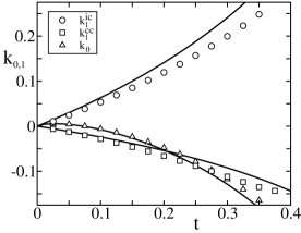
Figure 10: Contributions to the bending rigidity $k_{0}$ and $k_{1}$ in units of $k_{\rm B}T$ versus the reduced temperature distance to the critical point, $t$. Symbols are numerical results, the drawn lines are the gradient expansion approximation.

In Figure 10, $k_{0}$, $k_{1}^{ic}$ and $k_{1}^{cc}$ are shown as a function of the reduced temperature distance to the critical point, $t\!\equiv\!|1-T/T_{c}|$. The open symbols are obtained from numerically solving Eqs.(49) and (IV) to obtain $\rho_{0}(z)$ and $\rho_{1}(z)$ and inserting the result into Eqs.(91) and (92). The drawn lines are the gradient expansion approximation for $k_{0}$ in Eq.(94) and $k_{1}$ in Eq.(VI.1).

Adding the expressions for $k_{0}$ in Eq.(94) and $k_{1}$ in Eq.(VI.1), one obtains for $\ell_{k}$

$$\ell^{cc}_{k} = \exp(c_{0}+c^{cc}_{1})\,\xi+{\cal O}(d)$$

$$\approx 0.311942\ldots\,\xi+{\cal O}(d)\,,$$

$$\ell^{ic}_{k} = \exp(c_{0}+c^{ic}_{1})\,\xi+{\cal O}(d)$$ (100)

$$\approx 2.354329\ldots\,\xi+{\cal O}(d)\,.$$

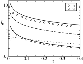
Figure 11: The bending length $\ell_{k}$ (in units of $d$) versus the reduced temperature distance to the critical point, $t$, using the integral constraint (circles) and crossing constraint (squares). Open symbols are numerical results, the drawn lines are the gradient expansion approximation. The dashed line is the correlation length $\xi$ and the dotted line is the Mecke and Dietrich result (Ref. Mecke, ) with $C_{\rm H}\!=\!1/4$.

In Figure 11, the bending length is shown as a function of $t$. The open symbols are the numerical results. The drawn lines are the gradient expansion approximations in Eq.(VI.1).

Other than that the gradient expansion seems not to be as accurate in reproducing numerical results, the results in Figures 10 and 11 are in line with the earlier results obtained for short-ranged forces. The leading order correction to the surface tension is negative when $q\ell_{k}\!<\!1$, and the effect is more pronounced for the crossing constraint than the integral constraint. Although the goal of Mecke and Dietrich in ref. Mecke, is to include higher order terms, terms beyond $q^{2}$ in the expansion of $\sigma(q)$, it is also interesting to compare with the Mecke and Dietrich approach for the terms obtained to order $q^{2}\,\ln(q)$ and $q^{2}$. Using the Mecke and Dietrich expression for $\rho_{1}(z)$ in Eq.(50), one has to leading order in the gradient expansion:

$$\sigma_{\rm MD}(q)\!\! = \!\!\sigma+k_{s}\,q^{2}\ln(qd)+k_{0}\,q^{2}+k_{\rm MD}\,q^{2}+..$$ (101)

$$\equiv \!\!\sigma+k_{s}\,q^{2}\,\ln(q\ell^{\rm MD}_{k})+{\cal O}(q^{4})\,,$$

where $k_{s}$ and $k_{0}$ are given by the expressions in Eq.(92) and Eq.(94), and where $k_{\rm MD}$ is given by the previously derived expression in Eq.(85) for short-ranged forces. In Figure 11, we show, as the dotted line, the result for the bending length $\ell_{k}^{\rm MD}$.

VII Discussion

In the first part of this article, we have demonstrated that the full spectrum of surface fluctuations obtained in Monte Carlo simulations Vink of the colloid-polymer interface, can very accurately be described by the following expression:

$$S(q)=\frac{k_{\rm B}T}{\sigma\,q^{2}}-\frac{k\,\,k_{\rm B}T}{\sigma^{2}}+{\cal N}_{L}\,S_{b}(q)\,.$$ (102)

The three terms in this expression work in three different $q$-regimes:

1. Classical capillary wave regime, $qd\!\ll\!1$

2. Extended capillary wave regime, $qd\!\apprle\!1$

3. Bulk-like fluctuations regime, $qd\!\apprge\!1$

Two adjustable parameters are present: ${\cal N}_{L}$ that weighs the bulk-like fluctuations compared to the capillary wave fluctuations and the bending rigidity $k$ as defined by the leading order correction in an expansion of $\sigma(q)$ in $q^{2}$, $\sigma(q)\!=\!\sigma+k\,q^{2}+\ldots$. We found that a fit to the simulation results yields $k\!<\!0$, i.e. the leading order curvature correction tends to lower the surface tension $\sigma(q)$. This effect is termed capillary enhancement Daillant ; capillary waves are “more violent”, less restricted by surface tension, at smaller wavelengths.

One could worry whether a negative bending rigidity is consistent with having a stable interface. Tarazona et al. Tarazona indicate that a decrease of $\sigma(q)\!=\!\sigma+k\,q^{2}+\ldots$ ultimately leads to a destabilisation of the interface at large $q$. It is therefore important to realise that the extension of the capillary wave model, through the inclusion of a bending rigidity, is valid only for low $q$. Higher order terms in the expansion in $q$ are not systematically included. In this article we propose to describe $S(q)$ for large $q$ ($qd\!\apprge\!1$) in terms of molecular, bulk-like fluctuations through $S_{b}(q)$. It is shown that the full $S(q)$, which is then a combination of the extended capillary wave model at low $q$ and bulk-like fluctuations at large $q$, remains well-behaved ensuring the stability of the interface. For systems with a low (or even zero) surface tension, the bending rigidity is the dominant contribution near $q\!=\!0$ and one necessarily requires a positive value for $k$ Safran , but for the simple, (quasi) one-component system considered here this is not an issue.

A most important and generally underappreciated point that we like to emphasize is that the location of the interface cannot be defined unambiguously. A certain procedure must always be formulated to determine the height function $h(\vec{r}_{\parallel})$. We have shown that different choices for the location of the interface, which are all equally legitimate as long as they lead to a location of the dividing surface that is ‘sensibly coincident’ with the interfacial region Gibbs , lead to different results for the bending correction to the capillary wave model. Naturally, all experimentally measurable quantities cannot depend on the chosen location of the interface, making it necessary to formulate precisely the quantity that is determined in experiments or simulations. It was shown that for the simulation results, the value of the bending rigidity in the above expression for $S(q)$, corresponds to the height function being defined according to the integral constraint, $k\!=\!k^{ic}$.

For the determination of $k$, it is necessary to take the contribution from bulk-like fluctuations into account since they also contribute as a constant, ${\cal N}_{L}\,S_{b}(0)$, in the capillary wave regime ($qd\!\ll\!1$). This observation is consistent with the interpretation of light scattering results by Daillant and coworkers Daillant . To determine $\sigma(q)$, they subtract from $S(q)$ a contribution proportional to the penetration depth ($\propto{\cal N}_{L}$) times the liquid compressibility ($\propto S_{b}(0)$). Even though the light scattering results by Daillant Daillant are obtained for real fluids, for which the interaction potential is not necessarily short-ranged, one expects that a description in terms of the above mentioned three regimes is again useful. A further comparison with the light scattering results is, however, necessary.

In the second part of this article, a molecular theory to describe the inclusion of the bending rigidity correction to the capillary wave model is presented. An essential feature of the theory is the ‘Ansatz’ made in Eq.(53) regarding the thermodynamic conditions used to vary the interfacial curvature. It improves on earlier choices made in the sense that the bulk densities are equal to those at coexistence and the density profile is a continuous function Blokhuis92 ; Parry94 ; Blokhuis99 ; FJ . The theory predicts that the scaling behavior of the bending rigidity equals that of the surface tension near the critical point

$$k\,\propto\,\sigma\,d^{2}\,\propto\,t^{\mu}\,,$$ (103)

where $\mu\!\approx\!1.26$ is the usual surface tension critical exponent (in mean-field $\mu\!=\!3/2$) RW . This new scaling prediction differs fundamentally from the scaling of the bending rigidity in the ‘equilibrium approach’, $k_{\rm eq}\!\propto\!\sigma\,\xi^{2}$. In this approach the bending rigidity is determined from considering the equilibrium free energy of spherically and cylindrically shaped liquid droplets, with their radii varied by changing the value of the system’s chemical potential Blokhuis93 ; Gompper ; Giessen .

The negative sign and scaling behavior of the bending rigidity obtained from the molecular theory are in accord with Monte Carlo simulations. However, the magnitude of $k$ from the molecular theory, $\sqrt{-k/\sigma}\approx$ 0.13 $d$, is significantly below the value obtained in the simulations, $\sqrt{-k/\sigma}\approx$ 0.47 $d$ (see also Figure 8), but we believe this to be due to simplifications made in the theory rather than a true discrepancy.

Acknowledgment I am indebted to Dick Bedeaux for arguing with me on this intriguing topic since already 20 years. My thoughts have furthermore been shaped by discussions with giants in this field: John Weeks, Ben Widom, and Bob Evans. I would like to express my gratitude to Richard Vink for sharing unpublished simulation results and to Daniel Bonn, Didi Derks and Joris Kuipers for discussions on the colloid-polymer system.

Appendix A Depletion interaction potential

The phase-separated colloid-polymer system is effectively treated as a one-component system considering the colloids only. The colloid-colloid interaction is then given by a hard sphere repulsion (diameter $d$) with an attractive depletion interaction AOVrij induced by the presence of polymers (radius $R_{\rm g}$):

$$U_{\rm dep}(r)=\frac{-k_{\rm B}T\,\eta_{p}}{2\,(\varepsilon-1)^{3}}\left[\,2\,\varepsilon^{3}-3\,\varepsilon^{2}\left(\frac{r}{d}\right)+\left(\frac{r}{d}\right)^{\!3}\,\right]$$ (1)

with $d\!<\!r\!<\!\varepsilon d$ and the size ratio parameter $\varepsilon$ is defined as:

$$\varepsilon\equiv 1+\frac{2R_{\rm g}}{d}\,.$$ (2)

Using this form for $U_{\rm att}(r)$, the coefficients $a$, $m$, $B$ are readily calculated to yield

$$a = k_{\rm B}T\,d^{3}\,\eta_{p}\,\frac{\pi}{12}\,(2+6\,\varepsilon+3\,\varepsilon^{2}+\varepsilon^{3})\,,$$

$$m = k_{\rm B}T\,d^{5}\,\eta_{p}\,\frac{\pi}{240}\,(5+15\,\varepsilon+10\,\varepsilon^{2}+6\,\varepsilon^{3}$$ (3)

$$\hskip 65.0pt+3\,\varepsilon^{4}+\varepsilon^{5})\,,$$

$$B = k_{\rm B}T\,d^{7}\,\eta_{p}\,\frac{\pi}{8400}\,(28+84\,\varepsilon+63\,\varepsilon^{2}$$

$$\hskip 20.0pt+45\,\varepsilon^{3}+30\,\varepsilon^{4}+18\,\varepsilon^{5}+9\,\varepsilon^{6}+3\,\varepsilon^{7})\,.$$

One may also determine the functions $w_{0}(z_{12})$, $w_{2}(z_{12})$ and $w_{4}(z_{12})$. When $|z_{12}|\!<\!d$ one has:

$$w_{0}(z_{12})=-k_{\rm B}T\,d^{2}\,\eta_{p}\,\frac{\pi}{5}\,(1+3\,\varepsilon+\varepsilon^{2})\,,$$

$$w_{2}(z_{12})=k_{\rm B}T\,d^{4}\,\eta_{p}\,\frac{\pi}{280}\,\bigl{[}10+30\,\varepsilon+18\,\varepsilon^{2}$$

$$\hskip 20.0pt+9\,\varepsilon^{3}+3\,\varepsilon^{4}-14\,\left(1+3\,\varepsilon+\varepsilon^{2}\right)\,\frac{z_{12}^{2}}{d^{2}}\bigr{]}\,,$$

$$w_{4}(z_{12})=-k_{\rm B}T\,d^{6}\,\eta_{p}\,\frac{\pi}{20160}\times$$

$$\Bigl{[}\,5(7+21\,\varepsilon+15\,\varepsilon^{2}+10\,\varepsilon^{3}+6\,\varepsilon^{4}+3\,\varepsilon^{5}+\varepsilon^{6})$$

$$\hskip 10.0pt-9\,\left(10+30\,\varepsilon+18\,\varepsilon^{2}+9\,\varepsilon^{3}+3\,\varepsilon^{4}\right)\,\frac{z_{12}^{2}}{d^{2}}$$

$$\hskip 10.0pt+63\,\left(1+3\,\varepsilon+\varepsilon^{2}\right)\,\frac{z_{12}^{4}}{d^{4}}\Bigr{]}\,.$$ (4)

When $d\!<\!|z_{12}|\!<\!\varepsilon d$ one has:

$$w_{0}(z_{12})=\frac{-k_{\rm B}T\,d^{2}\,\eta_{p}}{(\varepsilon-1)^{3}}\,\frac{\pi}{5}$$

$$\hskip 1.0pt\times\left[\varepsilon^{5}-5\,\varepsilon^{3}\,\frac{z_{12}^{2}}{d^{2}}+5\,\varepsilon^{2}\,\frac{|z_{12}|^{3}}{d^{3}}-\frac{|z_{12}|^{5}}{d^{5}}\right]\,,$$

$$w_{2}(z_{12})=\frac{k_{\rm B}T\,d^{4}\,\eta_{p}}{(\varepsilon-1)^{3}}\,\frac{\pi}{280}$$

$$\hskip 1.0pt\times\left[3\,\varepsilon^{7}-14\,\varepsilon^{5}\,\frac{z_{12}^{2}}{d^{2}}+35\,\varepsilon^{3}\,\frac{z_{12}^{4}}{d^{4}}-28\,\varepsilon^{2}\,\frac{|z_{12}|^{5}}{d^{5}}\right.$$

$$\hskip 120.0pt\left.+4\,\frac{|z_{12}|^{7}}{d^{7}}\right]\,,$$

$$w_{4}(z_{12})=\frac{-k_{\rm B}T\,d^{6}\,\eta_{p}}{(\varepsilon-1)^{3}}\,\frac{\pi}{20160}$$

$$\hskip 1.0pt\times\left[5\,\varepsilon^{9}-27\,\varepsilon^{7}\,\frac{z_{12}^{2}}{d^{2}}+63\,\varepsilon^{5}\,\frac{z_{12}^{4}}{d^{4}}-105\,\varepsilon^{3}\,\frac{z_{12}^{6}}{d^{6}}\right.$$

$$\hskip 60.0pt\left.+72\,\varepsilon^{2}\,\frac{|z_{12}|^{7}}{d^{7}}-8\,\frac{|z_{12}|^{9}}{d^{9}}\right]\,.$$ (5)

Appendix B London-dispersion forces

The following explicit form for $U_{\rm att}(r)$ is considered:

$$U_{\rm att}(r)=\left\{\begin{array}[]{cl}-A/r^{6}&\hskip 10.0pt{\rm when}\hskip 10.0ptr>d\,,\\ 0&\hskip 10.0pt{\rm when}\hskip 10.0ptr<d\,.\end{array}\right.$$ (1)

Using this form for $U_{\rm att}(r)$, the coefficients $a$ and $m$ are readily calculated to yield

$$a=\frac{2\pi A}{3\,d^{3}}\hskip 20.0pt{\rm and}\hskip 20.0ptm=\frac{\pi A}{3\,d}\,.$$ (2)

With this form for the interaction potential one may expand $\omega(q,z_{12})$. When $|z_{12}|\!>\!d$ one has:

$$\omega(q,z_{12})=-\frac{\pi A}{2\,z_{12}^{4}}+\frac{\pi A}{8\,z_{12}^{2}}\,q^{2}+\frac{\pi A}{32}\,q^{4}\,\ln(qd)$$

$$+\frac{\pi A}{32}\,q^{4}\left[\,\gamma_{\rm E}-\frac{3}{4}+\frac{1}{2}\ln\!\!\left(\frac{z_{12}^{2}}{4d^{2}}\right)\,\right]+\ldots$$ (3)

When $|z_{12}|\!<\!d$ one has:

$$\omega(q,z_{12})=-\frac{\pi A}{2\,d^{4}}+\frac{\pi A}{8\,d^{2}}\,\left(2-\frac{z_{12}^{2}}{d^{2}}\right)\,q^{2}$$

$$+\frac{\pi A}{32}\,q^{4}\,\ln(qd)$$ (4)

$$+\frac{\pi A}{32}\,q^{4}\left[\gamma_{\rm E}-\frac{3}{2}-\ln(2)+\frac{z_{12}^{2}}{d^{2}}-\frac{z_{12}^{4}}{4d^{4}}\right]+\ldots$$

References

- (1) C. Fradin, A. Braslau, D. Luzet, D. Smilgies, M. Alba, N. Boudet, K. Mecke, and J. Daillant, Nature 403, 871 (2000); J. Daillant and M. Alba, Rep. Prog. Phys. 63, 1725 (2000); S. Mora, J. Daillant, K. Mecke, D. Luzet, A. Braslau, M. Alba and B. Struth, Phys. Rev. Lett. 90, 216101 (2003).
- (2) J. Stecki and S. Toxvaerd, J. Chem. Phys. 103, 9763 (1995).
- (3) R.L.C. Vink, J. Horbach and K. Binder, J. Chem. Phys. 122, 134905 (2005).
- (4) P. Tarazona, R. Checa, and E. Chacon, Phys. Rev. Lett. 99, 196101 (2007).
- (5) R. Evans, in Liquids at Interfaces, Les Houches XLVIII (1988), eds. J. Charvolin, J.F Joanny, and J. Zinn-Justin (North-Holland, Amsterdam, 1990).
- (6) J.R. Henderson in Fundamentals of Inhomogeneous Fluids (D. Henderson, ed.), Dekker, New York (1992).
- (7) J.S. Rowlinson and B. Widom, Molecular Theory of Capillarity (Clarendon, Oxford 1982).
- (8) F.P. Buff, R.A. Lovett and F.H. Stillinger, Phys. Rev. Lett. 15, 621 (1965).
- (9) J.D. Weeks, J. Chem. Phys. 67, 3106 (1977).
- (10) D. Bedeaux and J.D. Weeks, J. Chem. Phys. 82, 972 (1985).
- (11) W. Helfrich, Z. Naturforsch. 28C, 693 (1973).
- (12) J. Meunier, J. Physique 48, 1819 (1987); H. Kellay, B.P. Binks, and J. Meunier, Phys. Rev. Lett. 70, 1485 (1993); H. Kellay and J. Meunier, J. Phys. Condens. Matter 8, A49 (1996).
- (13) E.M. Blokhuis and D. Bedeaux, Physica A 164, 515 (1990); J.W. Schmidt, Phys. Rev. A 38, 567 (1988).
- (14) E.M. Blokhuis, J. Kuipers, and R.L.C. Vink, Phys. Rev. Lett. 101, 086101 (2008).
- (15) S. Asakura and F. Oosawa, J. Chem. Phys. 22, 1255 (1954); A. Vrij, Pure Appl. Chem. 48, 471 (1976).
- (16) A.P. Gast, C.K. Hall and W.B. Russel, J. Coll. Interface Sci. 96, 251 (1983).
- (17) H.N.W. Lekkerkerker, W.C.K. Poon, P.N. Pusey, A. Stroobants and P.B. Warren, Europhys. Lett. 20, 559 (1992).
- (18) D.G.A.L. Aarts and H.N.W Lekkerkerker, J. Phys. Cond. Matt. 16, S4231 (2004); D.G.A.L. Aarts, M. Schmidt and H.N.W. Lekkerkerker, Science 304, 847 (2004).
- (19) K.R. Mecke and S. Dietrich, Phys. Rev. E. 59, 6766 (1999).
- (20) E.M. Blokhuis and D. Bedeaux, Mol. Phys. 80, 705 (1993).
- (21) A.O. Parry and C.J. Boulter, J. Phys. Condens. Matter 6, 7199 (1994).
- (22) E.M. Blokhuis, J. Groenewold and D. Bedeaux, Mol. Phys. 96, 397 (1999).
- (23) J.W. Gibbs, Collected works (Dover, New York, 1961).
- (24) E.M. Blokhuis and D. Bedeaux, Physica A 184, 42 (1992); E.M. Blokhuis and D. Bedeaux, Heterog. Chem. Rev. 1, 55 (1994).
- (25) G. Gompper and S. Zschocke, Phys. Rev. A 46, 4386 (1992); G. Gompper and M. Schick, Self-assembling amphiphilic system, Phase Transitions and Critical Phenomena 16, C. Domb and J. Lebowitz eds. (Academic Press, London, 1994).
- (26) J.K. Percus and G.J. Yevick, Phys. Rev. 110, 1 (1958).
- (27) A.O. Parry , C. Rascón, N.R. Bernardino, and J.M. Romero-Enrique, Phys. Rev. Lett. 100, 136105 (2008); J. Phys. Condens. Matter 18, 6433 (2006); J. Phys. Condens. Matter 19, 416105 (2007).
- (28) H.N.W. Lekkerkerker, Colloids and Surfaces 51, 419 (1990).
- (29) N.F. Carnahan and K.E. Starling, J. Chem. Phys. 51, 635 (1969).
- (30) M.E. Fisher and A. Jin, Phys. Rev. B 44, 1430 (1991); Phys. Rev. Lett. 69, 792 (1992); A.J. Jin and M.E. Fisher, Phys. Rev. B 47, 7365 (1993).
- (31) J. Kuipers and E.M. Blokhuis, J. Coll. Interf. Sci. 315, 270 (2007).
- (32) C. Varea and A. Robledo, Mol. Phys. 85, 477 (1995).
- (33) M. Napiórkowski and S. Dietrich, Phys. Rev. E 47, 1836 (1993); M. Napiórkowski and S. Dietrich, Z. Phys. B 97, 511, (1995).
- (34) R.H. Fowler, Proc. R. Soc. Lond. A 159, 229 (1937).
- (35) S.A. Safran, Statistical Thermodynamics of Surfaces, Interfaces and Membranes (Reading, MA: Addison-Wesley, 1994).
- (36) A.E. van Giessen and E.M. Blokhuis, J. Chem. Phys. 116, 302 (2002).