Cross-calibration of cluster mass-observables

Abstract

This paper is a first step towards developing a formalism to optimally extract dark energy information from number counts using multiple cluster observation techniques. We use a Fisher matrix analysis to study the improvements in the joint dark energy and cluster mass-observables constraints resulting from combining cluster counts and clustering abundances measured with different techniques. We use our formalism to forecast the constraints in $\Omega_{\rm DE}$ and $w$ from combining optical and SZ cluster counting on a 4000 sq. degree patch of sky. We find that this cross-calibration approach yields $\sim 2$ times better constraints on $\Omega_{\rm DE}$ and $w$ compared to simply adding the Fisher matrices of the individually self-calibrated counts. The cross-calibrated constraints are less sensitive to variations in the mass threshold or maximum redshift range. A by-product of our technique is that the correlation between different mass-observables is well constrained without the need of additional priors on its value.

I Introduction

The evolution of the number of clusters of galaxies provides a powerful tool to study the nature of dark energy. Clusters are sensitive probes of the growth of structure because cluster abundances are exponentially dependent on the linear density perturbation field. In addition, cluster surveys are sensitive to the evolution of the volume element with redshift so that cluster surveys also probe the background cosmology.

Planned and ongoing cluster surveys will detect millions of clusters using a variety of techniques such as counts of optically detected galaxies (e.g. DES The Dark Energy Survey Collaboration (2005), LSST, Tyson and Wolff (2002)), the Sunyaev-Zel’dovich (SZ) flux decrement (e.g. SPT Ruhl et al. (2004) and ACT Kosowsky (2003)), X-ray temperature and surface brightness (e.g. eRosita, Predehl et al. (2007)), and weak lensing shear. Because different cluster techniques suffer from different sources of errors, combining the information from different surveys is essential to reduce random errors and control the systematics.

One of the major challenges in extracting dark energy information from clusters is that cluster masses are not directly observable. One must rely on observable proxies for mass which only correlate statistically with the true mass. The inherent uncertainties in the observable-mass relation will degrade cosmological constraints if not well understood. Methods have been developed to use additional cluster properties such as the cluster power spectrum (Majumdar and Mohr, 2004), sample covariance from counts in cells (Lima and Hu, 2004), or the shape of the observed mass function (Lima and Hu, 2005; Hu and Kravtsov, 2003; Rozo et al., 2007; Levine et al., 2002) to “self-calibrate” the mass-observable relation by simultaneously solving for the cosmological and mass-observable parameters.

Other works have investigated combining different cluster techniques to cross-calibrate the mass-observable relations of each (Majumdar and Mohr, 2004, 2003; Younger et al., 2006). In Majumdar and Mohr (2004, 2003), the cross-calibration is between an SZ or X-ray survey and a detailed mass follow-up to calibrate the mass-observable relation, whereas Younger et al. (2006) combine SZ and X-ray surveys. However, these studies have assumed that the two surveys were independent, so that the joint constraints were estimated by adding the Fisher matrices of both experiments. But if two surveys observe the same patch of sky, the measurements are not independent. The goal of this paper is to show how to exploit the interdependence of cluster surveys over the same patch of sky to improve constraints on dark energy and mass-nuisance parameters.

The paper is organized as follows. In §II we describe the Fisher matrix formalism to forecast cosmological constraints from cluster counts and clustering using a single and multiple observables. We describe the major cluster mass determination techniques in §III and explain our parametrization of the errors in the observables, i.e. the mass-observable distributions. Results are presented in §IV and our conclusions and prospects for future work are given in §V.

II Self-calibration and the Fisher matrix formalism

In this section we review how to obtain cosmological constraints from cluster counts and clustering using a single or multiple observables. Combining counts and clustering to derive cosmological constraints from a single mass estimation technique is often referred to as self-calibration.

II.1 Mean number counts

The use of clusters of galaxies as cosmological indicators depends on how reliably N-body simulations can predict the number density of dark matter halos associated to clusters of a given mass given an initial power spectrum. We adopt the fitting function of Jenkins et al. (2001) for differential comoving number density of clusters

$$\frac{d\bar{n}}{d\ln M}=0.3\frac{\rho_{m}}{M}\frac{d\ln\sigma^{-1}}{d\ln M}\exp[-|\ln\sigma^{-1}+0.64|^{3.82}],$$ (1)

where $\sigma^{2}(M,z)$ is the variance of the density field in a spherical region with mean (present-day) matter density $\rho_{m}$ encircling a mass $M$. Even though more recent fitting-functions exist (e.g. Tinker et al. (2008); Warren et al. (2006)), we adopt the above for easier comparison with the literature (e.g. Lima and Hu (2007, 2005, 2004)) and because the results are relatively insensitive to the fiducial mass function used.

Eq. (1) shows that the number density of clusters is sensitive to the variance of the density field, and hence to the initial power spectrum. However, uncertainties in the estimation of the mass are degenerate with changes in cosmological parameters. The utility of cluster number counts is therefore limited by uncertainties in the mass-observable relation. Results from both simulations (e.g. Shaw et al. (2007); Kravtsov et al. (2006)) and observations (e.g. (Rykoff et al., 2008a; Evrard et al., 2008; Rykoff et al., 2008b)) suggest that the mass-observable relations can be parametrized in simple forms with lognormal scatter of the mass-observable about the mean relation. Other works (see e.g. Cohn et al. (2007)) suggest that the distribution of galaxies in halos may be more complicated.

For $n$ observables, the probability of measuring clusters given the true mass $M$ and redshift $z$ is

$$p({\bf M^{\rm obs}},z^{\rm p}|M,z)\phi({\bf M^{\rm obs}},z^{\rm p}),$$ (2)

where ${\bf M^{\rm obs}}=({M^{\rm obs}_{1},M^{\rm obs}_{2},...,M^{\rm obs}_{n}})$ and $\phi(M^{\rm obs})$ is the combined selection function for all the observables. For simplicity, we always work in a range of redshift and mass where the surveys are expected to be nearly complete. This allows us to approximate the selection function as unity. This range depends on the observable we are using, so we postpone justifying our assumptions for survey selections to §III, when we describe the different cluster techniques. We further assume that the redshift errors are independent of the mass-observable errors. This assumption is not strictly true, since the bigger the cluster, the more bright optical galaxies it should have, and the better the cluster redshift estimate will be. This is particularly relevant for optical clusters, for which the cluster detection and mass estimate are inseparable from the cluster redshift determination. We will postpone dealing with this difficulty to a later work. For now, we write

$$p({\bf M^{\rm obs}},z^{\rm p}|M,z)=p({\bf M^{\rm obs}}|M)p(z^{\rm p}|z)$$ (3)

We define the probability of measuring the observable $M^{\rm obs}$ given the true mass $M$ as (Lima and Hu, 2005)

$$p(M^{\rm obs}|M)=\frac{1}{\sqrt{2\pi\sigma_{\ln M}^{2}}}\exp\left[-x^{2}(M^{\rm obs})\right],$$ (4)

where

$$x(M^{\rm obs})\equiv\frac{\ln M^{\rm obs}-\ln M-\ln M^{\rm bias}(M,z)}{\sqrt{2\sigma_{\ln M}(M,z)^{2}}}.$$ (5)

We describe our parametrization of $M^{\rm bias}(M,z)$ and $\sigma_{\ln M}(M,z)^{2}$ in §III when we discuss our modeling of different cluster techniques.

The number density of clusters at a given redshift $z$ with observable in the range $M^{\rm obs}_{\alpha}\leq M^{\rm obs}\leq M^{\rm obs}_{\alpha+1}$ is given by

$$\bar{n}_{\alpha}(z) \equiv \int_{M^{\rm obs}_{\alpha}}^{M^{\rm obs}_{\alpha+1}}\frac{dM^{\rm obs}}{M^{\rm obs}}\int{\frac{dM}{M}}{\frac{d\bar{n}}{d\ln M}}p(M^{\rm obs}|M)$$ (6)

where $x_{\alpha}=x(M^{\rm obs}_{\alpha})$.

We define the probability of measuring two observables $M^{\rm obs}_{a}$, $M^{\rm obs}_{b}$ given the true mass as a bivariate Gaussian distribution

$$p(M^{\rm obs}_{1},M^{\rm obs}_{2}|M)=\frac{1}{(2\pi)\det({\bf C})^{1/2}}\exp\left[-\frac{{\bf x}^{\rm T}{\bf C}^{-1}{\bf x}}{2}\right]$$ (7)

where $\bf C$ is the covariance matrix defined as

$${\bf C}=\begin{pmatrix}{\sigma}_{a}^{2}&\rho{\sigma}_{a}{\sigma}_{b}\\ \rho{\sigma}_{a}{\sigma}_{b}&{\sigma}_{b}^{2}\end{pmatrix}$$ (8)

and $\rho\in[-1,1]$ is the correlation coefficient. We motivate the use of the bivariate distribution in Appendix A.

At a given redshift $z$, the average number density of clusters with observables such that $M^{\rm obs}_{a,\alpha}\leq M^{\rm obs}_{a}\leq M^{\rm obs}_{a,\alpha+1}$ and $M^{\rm obs}_{b,\beta}\leq M^{\rm obs}_{b}\leq M^{\rm obs}_{b,\beta+1}$ is given by

$$\bar{n}_{\alpha,\beta}(z) \equiv \int_{M^{\rm obs}_{a,\alpha}}^{M^{\rm obs}_{a,\alpha+1}}\frac{dM^{\rm obs}_{a}}{M^{\rm obs}_{a}}\int_{M^{\rm obs}_{b,\beta}}^{M^{\rm obs}_{b,\beta+1}}\frac{dM^{\rm obs}_{b}}{M^{\rm obs}_{b}}\int\frac{dM}{M}\frac{d\bar{n}}{d\ln M}p(M^{\rm obs}_{a},M^{\rm obs}_{b}|M)$$ (9)

$$= \frac{\sqrt{\pi}}{8}\int\frac{dM}{M}\frac{d\bar{n}}{d\ln M}\int_{M^{\rm obs}_{a,\alpha}}^{M^{\rm obs}_{a,\alpha+1}}\frac{dM^{\rm obs}_{a}}{M^{\rm obs}_{a}}e^{-{x}_{a}^{2}}\left[{\rm erfc}\left(\rho x_{a}-x_{b}(M^{\rm obs}_{b,\beta})\over\sqrt{(1-\rho^{2})}\right)-{\rm erfc}\left(\rho x_{a}-x_{b}(M^{\rm obs}_{b,\beta+1})\over\sqrt{(1-\rho^{2})}\right)\right]$$

For the two observables case, the integrals over the observables can only be performed analytically if $\rho=0$. One would think that this problem could be resolved by diagonalizing the inverse covariance matrix - defined in Eq. (8). Diagonalization, however, does not simplify the calculation because the limits of the innermost integral over observables become dependent on the other observable. Thus, one cannot avoid performing the numerical integration. The equation for $b(z)$ is modified analogously to Eq. (9).

We interpret Eq. (9) as the combination of the error-free number density multiplied by two window-functions defined as:

$$W^{e}_{1}=e^{-{x}_{a}^{2}\over 2}$$ (10)

and

$$W^{e}_{2} = {\rm erfc}\left(\frac{\rho x_{a}-x_{b}(M^{\rm obs}_{b,\beta})}{\sqrt{2(1-\rho^{2})}}\right)$$ (11)

$$-{\rm erfc}\left(\frac{\rho x_{a}-x_{b}(M^{\rm obs}_{b,\beta+1})}{\sqrt{2(1-\rho^{2})}}\right).$$

Window $W^{e}_{1}$ has characteristic width given by the scatter of the observable $a$ with respect to the true mass, and is centered, in the $\ln M^{\rm obs}_{a}-\ln M$ coordinate, at the bias in the mass-observable relation, $\ln M^{\rm bias}_{a}$. The shape and position of window $W^{e}_{2}$ in $(\ln M^{\rm obs}_{a}-\ln M)$ depend on the value of the correlation coefficient $\rho$ as well as on the boundaries of the mass bin of the observable $b$, $M^{\rm obs}_{b,\beta}$ and $M^{\rm obs}_{b,\beta+1}$. If $\rho=0$, $W^{e}_{2}$ is simply a constant, independent of $M^{\rm obs}_{a}$ and $M$, as expected. For finite $\rho$, $W^{e}_{2}$ has the shape of a Mexican hat. As $|\rho|\rightarrow 1$, $W^{e}_{2}$ approaches a top-hat function, with edges at $x_{b}(M^{\rm obs}_{b,\beta})$ and $x_{b}(M^{\rm obs}_{b,\beta+1})$ for positive $\rho$ or at $-x_{b}(M^{\rm obs}_{b,\beta+1})$ and $-x_{b}(M^{\rm obs}_{b,\beta})$ for negative $\rho$. $W^{e}_{2}$ is not invariant under $\rho\rightarrow-\rho$ transformations. Decreasing $\rho$ “spreads out” the number counts in the $M^{\rm obs}_{a}-M^{\rm obs}_{b}$ plane. If the observables have different scatter, the spreading will be asymmetric with respect to the $M^{\rm obs}_{a}=M^{\rm obs}_{b}$ line. In other words, variations in $\rho$ are partially degenerate with both the scatter and bias of the different observables.

The mean cluster number counts are given by integrating Eq. (6) or (Eq. 9) over comoving volume. In spherical comoving coordinates, the volume element $dV$ is

$$dV=r^{2}drd\Omega=\frac{r^{2}(z)}{H(z)}dzd\Omega,$$ (12)

where $H(z)$ is the Hubble parameter at redshift $z$, $r(z)$ is the comoving angular diameter distance and $d\Omega$ is the differential solid angle. Uncertainties in the redshifts distort the volume element. Assuming photometric techniques are used to determine the redshifts of the clusters, we parametrize the probability of measuring a photometric redshift, $z^{\rm p}$, given the true cluster redshift $z$ as Lima and Hu (2007)

$$p(z^{\rm p}|z) = {1\over\sqrt{2\pi\sigma_{z}^{2}}}\exp\left[-y^{2}(z^{\rm p})\right],$$ (13)

where

$$y(z^{\rm p}) \equiv \frac{z^{\rm p}-z-z^{\rm bias}}{\sqrt{2\sigma_{z}^{2}}}$$ (14)

and $z^{\rm bias}=z^{\rm bias}(z)$ is the photometric redshift bias and $\sigma_{z}^{2}=\sigma_{z}^{2}(z)$ is the variance in the photo-z’s. We parametrize them as

$$z^{\rm bias}(z)\equiv z^{\rm bias}_{0}+d_{1}(1+z)$$ (15)

$$\sigma_{z}(z)\equiv\sigma^{0}_{z}+e_{1}(1+z)$$ (16)

For this paper we set the fiducial values $z^{\rm bias}_{0}=d_{1}=e_{1}=0$, and $\sigma^{0}_{z}=0.02$, the expected overall scatter of cluster photo-z’s in the Dark Energy Survey (The Dark Energy Survey Collaboration, 2005). We hold these parameters fixed throughout.

Assuming perfect angular selection the mean number of clusters in a photo-z bin $z^{\rm p}_{i}\leq z^{\rm p}\leq z^{\rm p}_{i+1}$ is

$$\bar{m}_{\alpha,\beta,i} = \int_{z^{\rm p}_{i}}^{z^{\rm p}_{i+1}}dz^{\rm p}\int dV\bar{n}_{\alpha,\beta}W_{i}^{\rm th}(\Omega)p(z^{\rm p}|z)$$ (17)

where $W^{\rm th}_{i}(\Omega)$ is an angular top hat window function.

To simplify the notation, henceforth we use the index $\alpha$ to indicate bins of both observables.

II.2 Noise in counts

The number of clusters found in an angular/redshift bin can deviate from the mean counts because of Poisson noise and large scale structure clustering. Both effects must be included in any likelihood analysis. On cluster scales, the clustering of baryonic matter follows the linear density fluctuations of total matter $\delta(x)$ corrected by the linear bias. That is,

$$m_{\alpha,i}({\bf x}) = \bar{m}_{\alpha,i}[1+b_{\alpha,i}(z)\delta({\bf x})],$$ (18)

where $b_{\alpha,i}(z)$ is the average cluster linear bias defined as

$$b_{\alpha,i}(z) = \frac{1}{\bar{n}_{\alpha,i}(z)}\int\frac{d{M^{\rm obs}_{\alpha}}}{M^{\rm obs}_{\alpha}}\int\frac{d{M^{\rm obs}_{\beta}}}{M^{\rm obs}_{\beta}}\int\frac{dM}{M}$$ (19)

$$\times\frac{d\bar{n}_{\alpha,i}(z)}{d\ln M}b(M;z)p(M^{\rm obs}|M).$$

We adopt the $b(M;z)$ fit of Sheth and Tormen (1999):

$$b(M;z)=1+\frac{a_{c}\delta_{c}^{2}/\sigma^{2}-1}{\delta_{c}}+\frac{2p_{c}}{\delta_{c}[1+(a\delta_{c}^{2}/\sigma^{2})^{p_{c}}]}$$ (20)

with $a_{c}=0.75$, $p_{c}=0.3$, and $\delta_{c}=1.69$.

The sample covariance of counts $m_{\alpha,i}$ is, given by (Hu and Kravtsov, 2003)

$$S^{\alpha\beta}_{ij} = \langle(m_{\alpha,i}-\bar{m}_{\alpha,i})(m_{\beta,j}-\bar{m}_{\beta,j})\rangle$$ (22)

$$= b_{\alpha,i}\bar{m}_{\alpha,i}b_{\beta,j}\bar{m}_{\beta,j}$$

$$\times\int{d^{3}k\over(2\pi)^{3}}W_{i}^{*}({\bf k})W_{j}({\bf k})\sqrt{P_{i}(k)P_{j}(k)},$$

where $W_{i}^{*}(\bf k)$ is the Fourier transform of the top-hat window function and $P_{i}(k)$ is the linear power spectrum at the centroid of redshift bin $i$. Notice that, in contrast to Hu and Kravtsov (2003), we use $\sqrt{P_{i}(k)P_{j}(k)}$ instead of $P(k)$ at an average redshift. We do not notice significant differences from this change. In addition, for computational efficiency, we only calculate covariance terms for which $|i-j|\leq 1$ and set the remaining terms to zero. Going from Eq. (22) to Eq. (22) we assumed that the bias was approximately constant in each photo-z bin so that it could be removed from the integral. We only considered the sample covariance in bins of redshift, but the angular covariance also contains useful information. We postpone calculating the full sample covariance to a future work.

Following Lima and Hu (2007), we find that the window function $W_{i}^{*}(\bf k)$ in the presence of photo-z errors is given by

$$W_{i}(\bf k)= 2\exp{\left[ik_{\parallel}\left(r_{i}+\frac{{z^{\rm bias}_{i}}}{{H_{i}}}\right)\right]}\exp{\left[-\frac{{\sigma_{z,i}^{2}k_{\parallel}^{2}}}{{2H_{i}^{2}}}\right]}$$ (23)

$$\times\frac{\sin(k_{\parallel}\delta r_{i}/2)}{k_{\parallel}\delta r_{i}/2}\frac{J_{1}(k_{\perp}r_{i}\theta_{s})}{k_{\perp}r_{i}\theta_{s}}.$$

Here $r_{i}=r(z^{\rm p}_{i})$ is the angular diameter distance to the $i^{\rm th}$ photo-z bin, and $\delta r_{i}=r(z^{\rm p}_{i+1})-r(z^{\rm p}_{i})$. Similarly, $H_{i}=H(z^{\rm p}_{i})=H(z)$, $z^{\rm bias}_{i}=z^{\rm bias}(z^{\rm p}_{i})=z^{\rm bias}(z)$, and $\sigma_{z,i}=\sigma_{z}(z^{\rm p}_{i})=\sigma_{z}(z)$. We assumed that $H(z)$, $z^{\rm bias}(z)$, and $\sigma_{z}(z)$ are constant inside each bin.

The Poisson noise of the counts is fully specified by the mean counts $\bar{m}$. The sample variance in the counts is determined by the mean counts, the bias, and the initial power spectrum. Since all these quantities can be predicted theoretically, both the mean counts and the sample variance contain useful information. In the following section we use the Fisher matrix formalism to estimate joint constraints for dark energy and mass-observable parameters using the information in the counts and the noise.

II.3 Fisher Matrix

Given a model specified by a set of parameters $p_{\alpha}$, with likelihood $L$, the Fisher information matrix is defined as

$$F_{\alpha\beta}=-\left\langle\frac{\partial^{2}{\rm ln}L}{\partial p_{\alpha}\partial p_{\beta}}\right\rangle$$ (24)

The marginalized errors in the parameters are given by $\sigma(p_{\alpha})=\left[(F^{-1})_{\alpha\alpha}\right]^{1/2}$. Priors are easily incorporated into the Fisher matrix. If parameter $p_{i}$ has a prior uncertainty of $\sigma(p_{i})$, we simply add $\sigma(p_{i})^{-2}$ to the $F_{ii}$ entry of the Fisher matrix before inverting.

Define the covariance matrix

$$C_{ij}=S_{ij}+{\bar{m}_{i}}\delta_{ij}$$ (25)

where ${\bar{m}_{i}}$ is the vector of mean counts defined in Eq. (17) and $S_{ij}$ is the sample covariance defined in Eq. (22). The indices $i$ and $j$ here run over all mass and redshift bins. Assuming Poisson noise and sample variance are the only sources of noise, the Fisher matrix is, (Hu and Cohn, 2006; Lima and Hu, 2004; Holder et al., 2001)

$$F_{\alpha\beta}=\bar{\bf m}^{t}_{,\alpha}{\bf C}^{-1}\bar{\bf m}_{,\beta}+{1\over 2}{\rm Tr}[{\bf C}^{-1}{\bf S}_{,\alpha}{\bf C}^{-1}{\bf S}_{,\beta}],$$ (26)

where the “,” denote derivatives with respect to the model parameters. The first term on the right-hand side contains the “information” from the mean counts, $\bar{m}$. The $S_{ij}$ matrix only contributes noise to this term, and hence only reduces its information content. The second term contains the information from the sample covariance.

For our purposes, the model parameters are the cosmological parameters, the parameters describing the errors in the observables (i.e. the mass nuisance parameters), and the parameters of the photo-z errors. We use two sets of fiducial cosmological parameters. One set is based on the first year data release of the Wilkinson Microwave Anisotropy Probe (WMAP1, Bennett et al. (2003)) and the other is based on the third-year data release (WMAP3, (Spergel et al., 2007)). We use WMAP1 and WMAP3 instead of the more recent five-year data release because the WMAP1 and WMAP3 are more extreme cases with regards to the value of $\sigma_{8}$ and the predicted number counts, and hence WMAP5 is more or less in-between both of them. The WMAP1 parameters assumed are: the baryon density, $\Omega_{b}h^{2}=0.024$, the dark matter density, $\Omega_{m}h^{2}=0.14$, the normalization of the power spectrum at $k=0.05{\rm Mpc}^{-1}$, $\delta_{\zeta}=5.07\times 10^{-5}$, the tilt, $n=1.0$, the optical depth to reionization, $\tau=0.17$, the dark energy density, $\Omega_{\rm DE}=0.73$, and the dark energy equation of state, $w=-1$. In this cosmology, $\sigma_{8}=0.91$. For WMAP3 we set $\Omega_{b}h^{2}=0.0223$, $\Omega_{m}h^{2}=0.128$, $\delta_{\zeta}=4.053\times 10^{-5}$ at $k=0.05{\rm Mpc}^{-1}$, $n=0.958$, $\tau=0.093$, $\Omega_{\rm DE}=0.73$, and $w=-1$. This cosmology corresponds to $\sigma_{8}=0.76$. With the exception of $w$, the cosmological parameters we used have been determined to an accuracy of a few percent. Extrapolating into the future, we assume $1\%$ priors on all cosmological parameters except $\Omega_{\rm DE}$ and $w$. We used CMBfast (Seljak and Zaldarriaga, 1996), version 4.5.1, to calculate the transfer functions.

III Cluster mass determination techniques

Figure 1: (Left) Mean counts as a function of redshift $\bar{m}(z)$ for various mass thresholds, with $\sigma_{\ln M}=0.25$ for both WMAP1 and WMAP3 cosmologies. (Right) $\bar{m}(z)$ for various values of $\sigma_{\ln M}$, with $M^{\rm th}=10^{14.2}h^{-1}M_{\odot}$ assuming a WMAP3 cosmology.

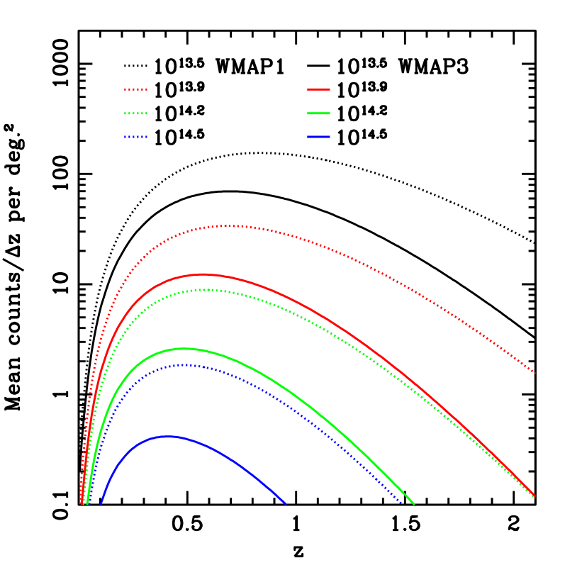
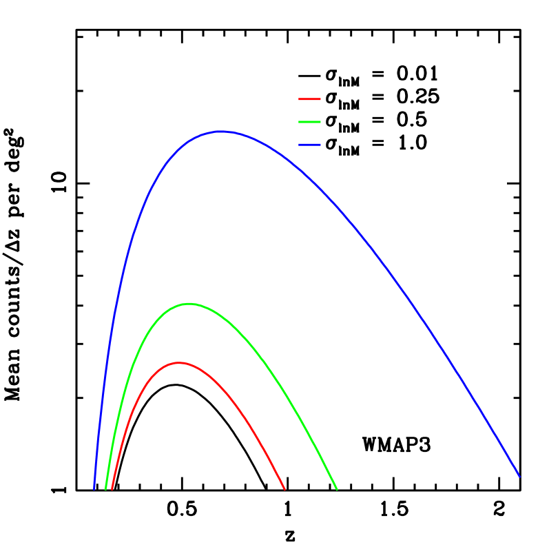
There are four commonly used cluster detection techniques for which large surveys are planned: optical, X-ray, Sunyaev-Zeldovich flux decrement, and weak lensing. For our Fisher matrix purposes, each of them is fully specified by a mass threshold, survey area, maximum redshift, and the parameters for the fiducial errors in $M^{\rm obs}$ and $z^{\rm p}$.

We show the mean number counts per redshift bin per sq. degree as a function of photometric redshift (with a constant scatter of $\sigma_{z}^{0}=0.02$) for several mass thresholds and scatters in Fig 1. The left plot shows the mean counts for $M^{\rm th}=10^{13.5}$, $10^{13.9}$, $10^{14.2}$, and $10^{14.2}h^{-1}M_{\odot}$, for a fixed scatter of $\sigma_{\ln M}=0.25$. The sensitivity of the counts to the mass threshold is apparent. The plot on the right shows the mean counts for $\sigma_{\ln M}=0.01$, $0.25$, $0.5$, $1.0$ with the threshold set to $M^{\rm th}=10^{14.2}h^{-1}M_{\odot}$. The increase of the scatter results in an increase in the total counts because the mass function falls exponentially with mass. It also causes flattening of the $\bar{m}(z)$ curve. The increase in the scatter implies an increase in the variance in counts, but a decrease in the shot noise. For perfectly known scatter, the decrease in shot noise outweighs the increase in variance implying that more scatter can yield better cosmological constraints. However, it is harder to constrain larger scatter and its evolution, and the assumption of Gaussianity may break down. This issue is particularly relevant for a WMAP3 cosmology, where there are fewer clusters compared to WMAP1.

Since the focus of this paper is on combining clusters in the same area of the sky, we limit our tests to surveys overlapping the South Pole Telescope (SPT) SZ Cluster survey. We thus set the area of the sky to 4000 square degrees, which we subdivide into 400 bins of 10 sq. degrees each. We assume SPT will be able to observe clusters with $M^{\rm obs}\geq 10^{14.2}h^{-1}M_{\odot}$ up to a redshift of 2 (see e.g. Carlstrom et al. (2002)). We assume that photometric redshifts will be available using DES+VISTA photometry. We parametrize the SZ mass bias and variance as

$${\rm ln}M^{\rm bias}(M,z) = {\rm ln}M^{\rm bias}_{0}+a_{1}(1+z)$$ (27)

$$= {\rm ln}M^{\rm bias}_{0}+{\rm ln}M^{\rm bias}(z)$$ (28)

$$\sigma_{\ln M}^{2}(M,z) = \sigma_{0}^{2}+\sum_{i=1}^{3}b_{i}z^{i}$$ (29)

$$= \sigma_{0}^{2}+\sigma_{\ln M}^{2}(z)$$ (30)

We set the fiducial mass scatter to $\sigma_{0}=0.25$, and all the other nuisance parameters to zero. In total, we use six nuisance parameters for the scatter and bias in mass (${\rm ln}M^{\rm bias}_{0}$, $a_{1}$, $\sigma_{0}^{2}$, $b_{i}$).

We assume a DES-like optical cluster survey with fiducial mass threshold of $M^{\rm th}=10^{13.5}h^{-1}M_{\odot}$ and maximum redshift of 1. Koester et al. (2007) and Johnston et al. (2007) were able to detect clusters with mass greater than $10^{13.5}h^{-1}M_{\odot}$ with a high level of purity and completeness using photometric data from the Sloan Digital Sky Survey (SDSS, (York, 2000)). The MaxBCG method used by these authors relies on red cluster galaxies occupying a distinct region in color space, the red sequence. The red sequence is known to be present in clusters at least to redshift of $1$ (see e.g. Gladders and Yee (2000)), so that we are justified in our choice for the expected DES mass threshold. Our choice of maximum redshift is somewhat conservative since with the addition of the IR filters from VISTA survey, DES+VISTA will have accurate redshifts (for field galaxies) up to $z\sim 1.5$. Conversely, the maximum redshift of 2 for SPT relies on the expectation that a deeper optical follow-up may be available for SPT-detected clusters. We show in §IV that if the cross-calibration is performed, the SZ clusters above $z\sim 1$ contribute very little to the cosmological constraints.

Different studies suggest a wide-range of scatter for optical observables, ranging from a constant $\sigma_{\ln M}=0.5$ (Wu et al., 2008) to a mass-dependent scatter in the range $0.75<\sigma_{\ln M}<1.2$ (Becker et al., 2007). After the submission of this paper, a couple of papers made more optimistic estimates for the scatter. Using weak lensing and X-ray analysis of MaxBCG selected optical clusters Rozo et al. (2008a) estimated a scatter of $\sim 0.45$ between weak lensing and optical richness estimates. In Rozo et al. (2008b) the authors show that improved richness estimators may reduce the optical scatter. As a conservative compromise, we choose a fiducial mass scatter of $\sigma_{\ln M}=0.5$ and allow for a cubic evolution in redshift and mass:

$${\rm ln}M^{\rm bias}(M,z) = {\rm ln}M^{\rm bias}_{0}+a_{1}(1+z)$$

$$+a_{2}({\rm ln}M^{\rm obs}-{\rm ln}M_{\rm pivot})$$

$$= {\rm ln}M^{\rm bias}_{0}+{\rm ln}M^{\rm bias}(z)+{\rm ln}M^{\rm bias}(M)$$

$$\sigma_{\ln M}^{2}(M,z) = \sigma_{0}^{2}+\sum_{i=1}^{3}b_{i}z^{i}$$

$$+\sum_{i=1}^{3}c_{i}({\rm ln}M^{\rm obs}-{\rm ln}M_{\rm pivot})^{i}.$$

$$= \sigma_{0}^{2}+\sigma_{\ln M}^{2}(M)+\sigma_{\ln M}^{2}(z)$$

We set $\ln(M_{\rm pivot})=34.5$ (with $M$ in units of $h^{-1}M_{\odot}$). In all, we have 10 nuisance parameters for the optical mass errors (${\rm ln}M^{\rm bias}_{0}$, $a_{1}$, $a_{2}$, $\sigma_{0}^{2}$, $b_{i}$, $c_{i}$). The results we obtain are sensitive to the choice of parametrization, particularly the number of nuisance parameters. There are few, if any, constraints on the number of parameters necessary to realistically describe the evolution of the variance and bias with mass for any technique. If simpler parametrizations than the ones we adopt here should prove to describe the variations in the errors well, than cosmological constraints would improve.

Figure 2: Optical-SZ mass bins in the redshift range (left) $0<z<1$ and (right) $1<z<2$. The black lines indicate the mass-threshold for the SZ and optical surveys. The gray lines show the boundaries of the mass bins. We do not use the SZ only region marked with the asterisk because there are very few clusters in that region.

III.1 Redshift/observables space

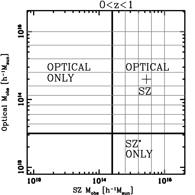
To calculate the SZ counts and sample variance, we use mass bins of width $\log(\Delta M^{\rm obs})=0.2$ with the exception of the highest mass bin, which we extend to infinity. We set the width of our redshift bins to $\Delta z^{\rm p}=0.1$. These bin sizes imply 5 bins of mass and 20 redshift bins for the SZ clusters. For the fiducial optical parameters, we divide the mass range $10^{13.5}\leq M^{\rm obs}_{\rm opt}\leq 10^{14.2}h^{-1}M_{\odot}$ into 5 bins and use the same mass binning as the SZ for $M^{\rm obs}_{\rm opt}>10^{14.2}h^{-1}M_{\odot}$, with a total of 10 mass bins and 10 redshift bins.

If the clusters detected by the optical and SZ surveys are in different parts of the sky, then the samples are independent. To estimate the joint constraints from both surveys one simply applies the single mass-observable analysis described in the previous section to each of the samples and sums the Fisher matrices.

If the clusters are all in the same part of the sky, then the samples are not independent. In addition, some regions of redshift/observable space contain clusters detected by both methods or only one. Our cross-calibration approach calculates the mean counts and clustering at all bins shown in Fig. 2. From Fig. 2 one can see that the observables parameter space is composed of four parts. One is defined as the set of clusters for which $10^{13.5}<M^{\rm obs}_{\rm opt}<10^{14.2}h^{-1}M_{\odot}$, $M^{\rm obs}_{\rm sz}<10^{14.2}h^{-1}M_{\odot}$, and $0<z<1$. Only optical clusters are detected in this region. We divide that interval of mass into 5 equally spaced bins and use $P(M^{\rm obs}_{\rm opt}|M)$ to estimate the counts in that region. The second region is defined as the clusters for which $M^{\rm obs}_{\rm sz}>10^{14.2}h^{-1}M_{\odot}$, $M^{\rm obs}_{\rm opt}>10^{13.5}h^{-1}M_{\odot}$ and $0<z<1$. The mass bins are simply the outer product of the optical and SZ vectors of bins of observables in that range. It is comprised of $5\times 10$ mass bins and $10$ redshift bins. Here we use $P(M^{\rm obs}_{\rm opt},M^{\rm obs}_{\rm sz}|M)$ to estimate the counts. The third region is defined by $M^{\rm obs}_{\rm sz}>10^{14.2}h^{-1}M_{\odot}$, $M^{\rm obs}_{\rm opt}<10^{13.5}h^{-1}M_{\odot}$ and $0<z<1$. Because there are almost no clusters detected in this region, we do not include it in our analysis. The fourth region is defined by $M^{\rm obs}_{\rm sz}>10^{14.2}h^{-1}M_{\odot}$ and $1<z<2$. Since only SZ clusters can be found in this region we estimate the counts using $P(M^{\rm obs}_{\rm sz}|M)$. The counts from the three regions we use are organized into a single vector of counts, and the corresponding covariance of the data (defined in Eq. 25) is given by a single matrix.

Fig. 1 hints that our choice of binning results in a large number of bins with mean counts substantially below unity. Such small number of clusters per bin brings about two concerns. The first is that in a real survey one would not be able to accurately estimate the mean of such bins. While this is true, our goal in this paper is to examine how much information is in the counts, which we can only be certain of extracting using a large number of bins. Our choice of binning does not yield overly optimistic results since the shot noise increases as the counts per bin become smaller. The bins with very few objects therefore do not contribute significantly to the Fisher matrix. We tested this using a total of 32 bins instead of 50 (in the region of overlap of the surveys) and found only negligible differences in the resulting dark energy constraints. When performing this analysis on real datasets, one would be advised to adopt a different binning strategy, perhaps using tree-structure algorithms to optimally subdivide the data, or hierarchical Bayesian classification algorithms, especially if more than two observables are used.

The second concern is that with few objects per bin the Gaussian approximation assumed when we defined Eq. (26) - see Lima and Hu (2004) for a derivation - is not valid. To test the impact of the Gaussian assumption, we performed the single-observable self-calibration analysis for the SZ survey using 5, 10, and 40 mass bins. The results are virtually identical if 5 or 10 bins are used, but degrade by a few percent for 40 bins. We did not investigate whether the degradation was a result of the breakdown of the Gaussian assumption or simply due to numerical noise. The important point is that excessive binning does not yield unrealistic improvements in the constraints.

IV Results

Unless stated otherwise, all results shown assume no priors on the nuisance parameters.

IV.1 Results for a single observable

Figure 3: Constraints on (left) $\Omega_{\rm DE}$ and (right) $w$ versus the maximum redshift of the survey for the fiducial optical and SZ surveys in WMAP1 and WMAP3 cosmologies.

Figure 4: Constraints on (left) $\Omega_{\rm DE}$ and (right) $w$ versus the mass threshold of the survey in a WMAP3 cosmology. The number of mass bins used in the calculation is different for each $M^{\rm th}$. At the lowest threshold $M^{\rm th}=10^{13.2}h^{-1}M_{\odot}$ and 16 bins of $M^{\rm obs}$ are used. We increase $M^{\rm th}$ in steps of $\Delta\ln M^{\rm obs}=0.1$ and decrease the number of mass bins by one at every step up to $M^{\rm th}=10^{14.7}h^{-1}M_{\odot}$. The solid black and solid gray lines are the marginalized constraints for the fiducial optical and SZ parametrizations. For the dashed black line we assume no mass dependence in the optical mass scatter, i.e. it uses the exact same parametrization as the fiducial SZ survey, except that $\sigma_{0}=0.5$ and the maximum redshift is 1.

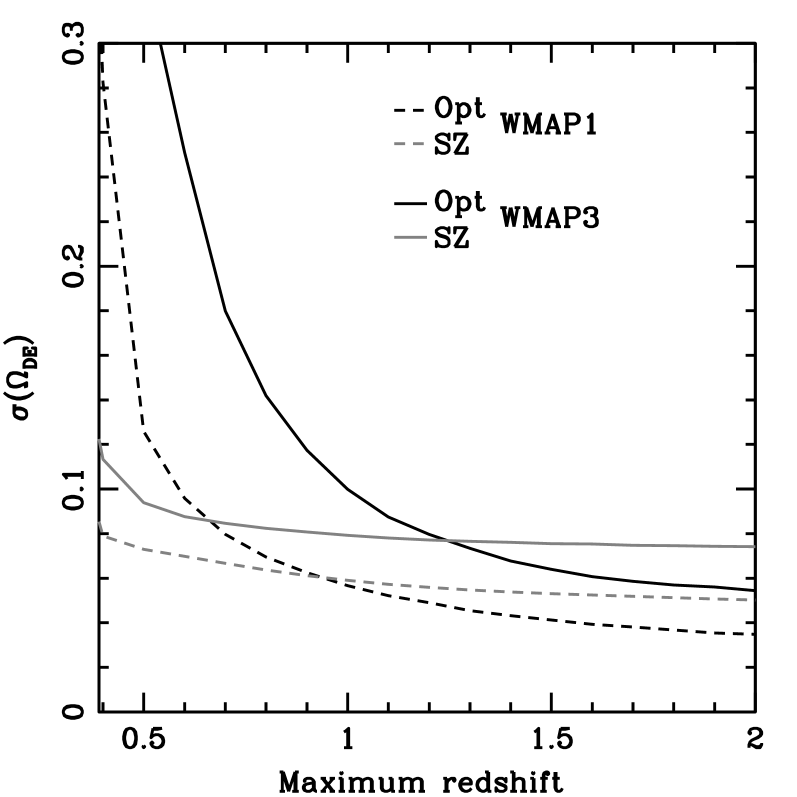
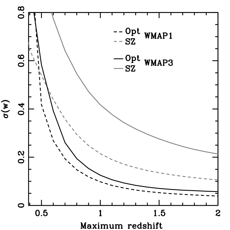
First, we present results for a single observable. Figure 3 shows the dependence of the constraints on $\Omega_{\rm DE}$ (left) and $w$ (right) on the maximum redshift of the survey ($z_{\rm max}$). The dashed and solid black lines are for the fiducial optical mass threshold, scatter and bias in WMAP1 and WMAP3 cosmologies, respectively. The dashed and solid gray lines are the corresponding results assuming the fiducial SZ survey. The rate of improvement in the $\Omega_{\rm DE}$ constraints with $z_{\rm max}$ decreases sharply after $z\sim 0.5$ for all cases except the optical results in WMAP3, where the break happens around $z\sim 1$. The constraints on $w$ show a more pronounced redshift dependence for both optical and SZ. In a WMAP3 cosmology, varying $z_{\rm max}$ from 1 to 2 results in $\sigma(w)$ decreasing by a factor of $\sim 2.5$ for the optical and $\sim 2.1$ for the SZ. The intersection of the dashed lines in both plots, or of the solid lines in the left plot mark the redshifts below which the optical survey yields tighter constraints than the SZ survey. At this point, Poisson noise in the counts is the dominant component of the error budget. The increase in counts due to the larger scatter of the optical observable compensates for the loss of information due to increased scatter.

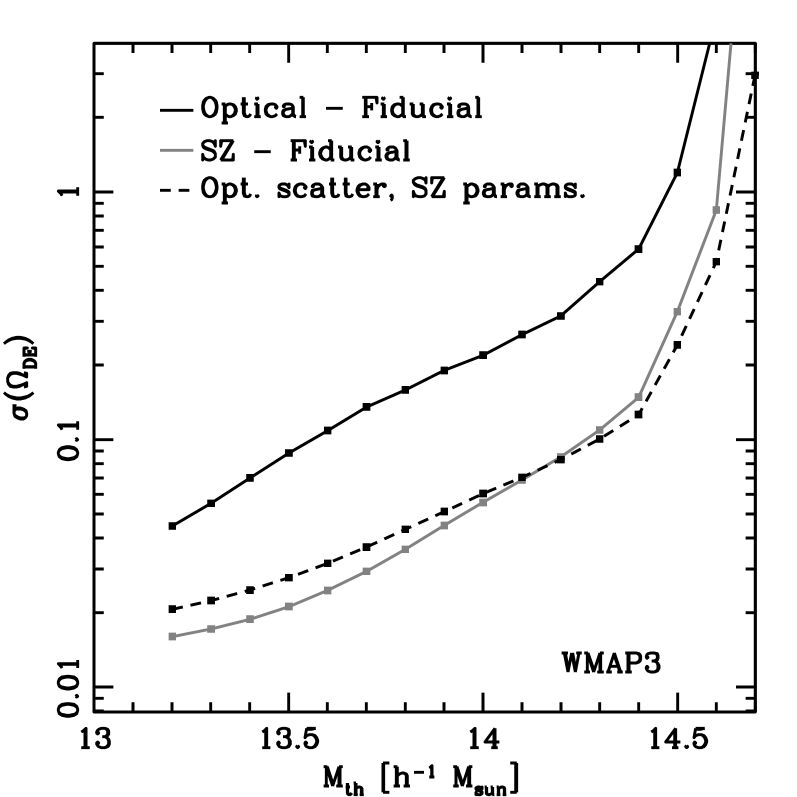
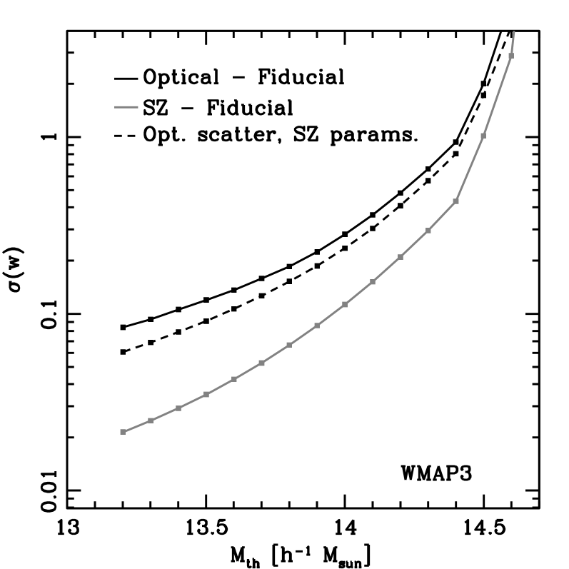
Figure 4 shows (left) $\sigma(\Omega_{\rm DE})$ and (right) $\sigma(w)$ versus the mass threshold of the survey in a WMAP3 cosmology. The number of mass bins used in the calculation is different for each $M^{\rm th}$. At the lowest threshold $M^{\rm th}=10^{13.2}h^{-1}M_{\odot}$ and there 16 bins of $M^{\rm obs}$. We increase $M^{\rm th}$ in steps of $\Delta\ln M^{\rm obs}=0.1$ and decrease the number of mass bins by one at every step up to $M^{\rm th}=10^{14.7}h^{-1}M_{\odot}$. The solid black and solid gray lines show the marginalized constraints for the fiducial optical and SZ parametrizations. For the dashed black line we assume no mass dependence in the optical mass scatter, i.e. we use the same parametrization as the fiducial SZ survey, except that $\sigma_{0}=0.5$, and the maximum redshift is 1. The fact that the dashed black line drops below the gray line in the left plot is another illustration of the point made in §III of larger scatter resulting in better cosmological constraints, despite the lower redshift range of the optical survey and no priors on the scatter. Allowing for mass dependence of $\ln M^{\rm bias}_{\rm opt}$ and $\sigma^{2}_{\rm opt}$ not only degrades $\sigma(\Omega_{\rm DE})$ but also increases the sensitivity of the constraints to $M^{\rm th}$. The constraints on $w$ are much less affected, because of the low maximum redshift of the optical survey.

IV.2 Results for two observables

Figure 5: $68\%$ confidence regions in the $\Omega_{\rm DE}-w$ plane in (left) WMAP1 and (right) WMAP3 cosmologies. The constraints from cross-calibration using only clusters detected simultaneously in optical and SZ (i.e. partial cross-calibration - with selection $M^{\rm obs}_{\rm sz}>10^{14.2}h^{-1}M_{\odot}$, $M^{\rm obs}_{\rm opt}>10^{13.5}h^{-1}M_{\odot}$ and $0<z<1$) are represented by the filled gray ellipses. The cross-calibration using all clusters (i.e. full cross-calibration) yields the filled black ellipses. For comparison, the long dashed red lines show constraints for the fiducial optical survey, and the short dashed blue lines show constraints for the fiducial SZ survey. Treating the optical and SZ surveys as independent and adding their Fisher matrices yields the solid black lines.

Figure 6: The filled light gray ellipse shows the constraints from summing the SZ and optical fisher matrices without clustering. The solid black line indicates the corresponding constraints when clustering is added. The filled dark gray and filled black ellipses show the full cross-calibration constraints without and with clustering, respectively.

Table 1: Marginalized constraints on cosmological parameters

	WMAP1		WMAP3
Survey	$\sigma(\Omega_{\rm DE})$	$\sigma(w)$	$\sigma(\Omega_{\rm DE})$	$\sigma(w)$
Intersection	0.058	0.093	0.070	0.15
Optical	0.057	0.098	0.10	0.13
SZ	0.050	0.11	0.074	0.21
Optical + SZ	0.032	0.062	0.057	0.092
Cross-Cal. (Full)c	0.021	0.030	0.025	0.045
Cross-Cal. ($z^{\rm SZ}_{max}<1.1$)c	0.022	0.032	0.026	0.047

^c Fixed $\rho=0$

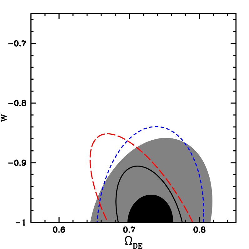
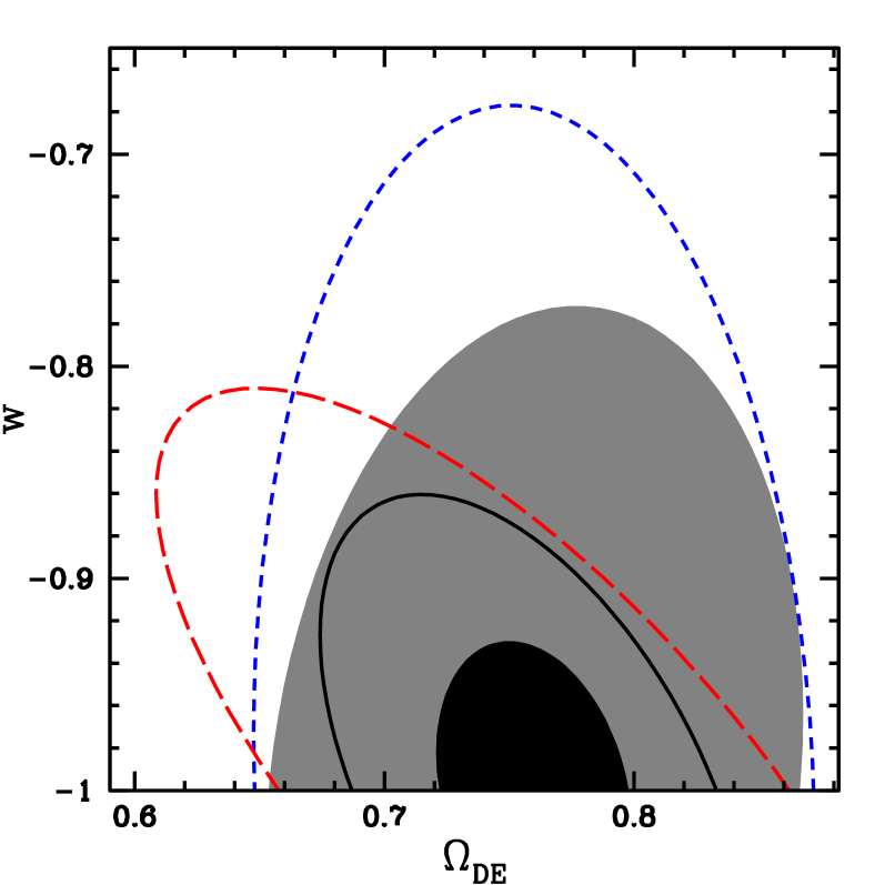
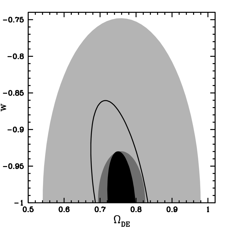
Figure 5 shows the $68\%$ confidence regions for $\Omega_{\rm DE}$ and $w$ in (left) WMAP1 and (right) WMAP3 cosmologies assuming no priors in the nuisance parameters and no correlation between the observables (i.e. $\rho=0$, fixed). Comparing both plots, we see that the low fiducial number of clusters in the WMAP3 cosmology implies weaker cosmological constraints. More interestingly, in a cosmology with fewer clusters the lower mass threshold of the optical technique makes it more constraining than the fiducial SZ even without any priors on the bias or scatter. The marginalized constraints are summarized in Table LABEL:tbl:constraints.

Performing the cross-calibration using only clusters detected by both methods (hereafter partial cross-calibration - represented in the plots by the filled gray ellipses) does not yield very good constraints. The partial cross-calibration is slightly more useful in a WMAP3 cosmology, because there are few clusters above $z=1$, so that not using that region of parameter space does not cause much degradation. Constraints using the cross-calibration with all clusters available (hereafter full cross-calibration - filled black ellipses) yields much better constraints than the partial cross-calibration. In fact, constraints on ${\Omega_{\rm DE}}$ and ${w}$ from the full cross-calibration are a factor $\sim 2$ better than constraints derived by simply adding the Fisher matrices of the optical and SZ techniques (the solid black line).

We demonstrate the importance of clustering in a WMAP3 cosmology to self- and cross-calibration in Fig. 6. Comparing the filled light gray ellipse with the solid black line, we see that clustering information tightens constraints on both $\Omega_{\rm DE}$ and $w$ significantly if we only sum the optical and SZ Fisher matrices. But comparing the filled dark gray ellipse with the filled black ellipse we see that clustering does not add as much information to the full cross-calibration. Constraints on $w$ are unchanged, and $\Omega_{\rm DE}$ constraints improve by a factor of $\sim 1.7$.

Figure 7: $\sigma(\Omega_{\rm DE})$ and $\sigma(w)$ for the full cross-calibration as a function of the optical mass threshold, $M_{\rm th}^{\rm opt}$ in both WMAP1 and WMAP3 cosmologies with correlation $\rho$ fixed at zero. The dots indicate boundaries of the mass bins for $M^{\rm obs}_{\rm opt}<10^{14.2}h^{-1}M_{\odot}$. Above $10^{14.2}$ we use the same bins as for $M^{\rm obs}_{\rm sz}$.

Figure 8: $\sigma(\Omega_{\rm DE})$ and $\sigma(w)$ for the full cross-calibration as a function of the maximum redshift of the optical survey, in WMAP1 and WMAP3 cosmologies with correlation $\rho$ fixed at zero.

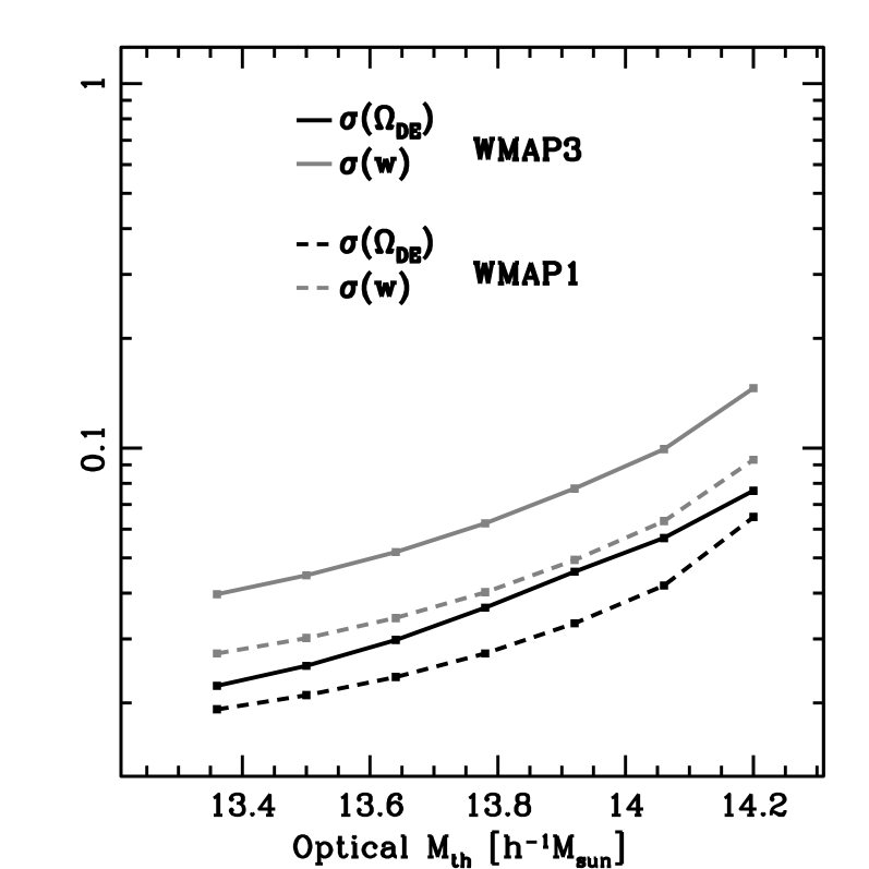
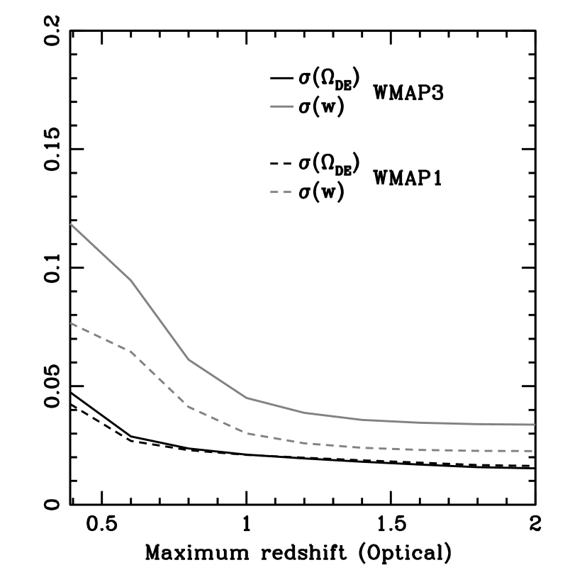
Figure 7 shows $\sigma(\Omega_{\rm DE})$ and $\sigma(w)$ for the full cross-calibration as a function of the optical mass threshold, $M_{\rm th}^{\rm opt}$, in both WMAP1 and WMAP3 cosmologies with $\rho$ fixed at zero. The dots indicate boundaries of the mass bins for $M^{\rm obs}_{\rm opt}<10^{14.2}h^{-1}M_{\odot}$. Above $10^{14.2}$ we use the same bins as the $M^{\rm obs}_{\rm sz}$. Constraints on $w$ are slightly less sensitive to $M^{\rm obs}_{\rm opt}$ than constraints on $\Omega_{\rm DE}$. Comparing the slopes of the curves in Figure 7 and Figure 4 we see that the full cross-calibration constraints are less sensitive to $M^{\rm th}$ than the self-calibrated constraints from optical or SZ alone. In Fig. 4 a change in $M^{\rm th}$ from $10^{13.5}h^{-1}M_{\odot}$ to $10^{14.2}h^{-1}M_{\odot}$ results in a degradation of $\sigma(w)$ and $\sigma(\Omega_{\rm DE})$ of $\sim 4.0$ and $\sim 3.6$, respectively, for optical only, and of $\sim 5.9$ and $\sim 4.0$ for SZ only. With the full cross-calibration, the degradation factor is only $\sim 3.0$ for $\sigma(\Omega_{\rm DE})$ and $\sim 3.3$ for $\sigma(w)$.

The full cross-calibration also reduces the sensitivity to the maximum redshift range of the surveys. Figure 8 shows $\sigma(\Omega_{\rm DE})$ and $\sigma(w)$ as a function of the maximum redshift of the optical survey for the full cross-calibration. Comparing to Figure 3 it is clear that the individual surveys are much more sensitive to $z_{\rm max}$ than the full cross-calibration. For example, if $z_{\rm max}$ changes from 1 to 2 in a WMAP3 cosmology, the optical-only and SZ-only constraints on $w$ improve by factors of $\sim 2.2$ and $\sim 2.0$, respectively. In comparison, the same change in $z_{\rm max}$ for the optical survey in the full cross-calibration improves $w$ constraints by only $\sim 1.3$. Cross-calibration constraints are even less sensitive to variations in the maximum redshift of the SZ survey. For a fixed optical $z_{\rm max}=1$, reducing the SZ $z_{\rm max}$ from $2$ to $1.1$ degrades constraints by only a few percent in both cosmologies. In this scenario, we find $\sigma(\Omega_{\rm DE},w)=(0.022,0.048)$ in a WMAP1 cosmology and $\sigma(\Omega_{\rm DE},w)=(0.027,0.073)$ in a WMAP3 cosmology.

All cross-calibration results shown heretofore assumed correlation coefficient $\rho$ fixed at zero. From Eq. (46) we see that $\rho=0$ implies $\sigma_{ab}=\sigma_{\rm opt-sz}=\infty$. Weak lensing and X-ray mass measurements of optically-selected clusters suggest that a more realistic guess would be $\sigma_{\rm opt-sz}\sim 0.3-0.7$, from which Eq. (46) implies that $0.19<|\rho|<0.55$. A value of $\rho>0.6$ corresponds to $\sigma_{\rm opt-sz}<0.19$. To obtain higher correlation values, one would need $\sigma_{ab}$ to be small compared to $\sigma_{a}$ and $\sigma_{b}$.

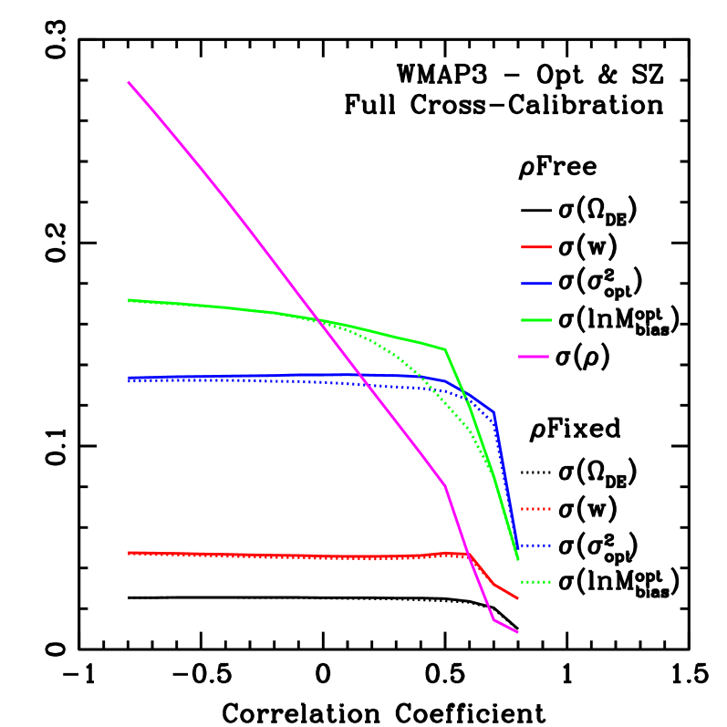
Figure (9) shows the dependence of the constraints on the dark energy and optical mass nuisance parameters on the correlation coefficient. From the left plot we see that the dark energy parameters are insensitive to the value of the correlation for $\rho<0.6$ for the full cross-calibration analysis. The very sharp drop in the uncertainties of both cosmological and nuisance parameters is largely due to the optical and SZ surveys having different fiducial scatters and mass thresholds. Given $\sigma_{\rm opt}$ and $\sigma_{\rm SZ}$, high values of the correlation imply very low values of $\sigma_{\rm opt-sz}$, the scatter between observables. High correlation means that the scatter in the optical is effectively that of the SZ survey. From the plot we see that $\rho=0.8$, the combination of optical and SZ results yields constraints very similar to a survey with optical $M^{\rm th}$ but with SZ scatter (cf. Fig. 4).

The constraints on $\rho$ improve as $\rho$ increases, though comparing constraints for fixed and free $\rho$, we see that dark energy constraints are fairly insensitive to $\sigma(\rho)$. This means that the correlation is sufficiently well determined by the cross-calibration analysis without need for additional priors.

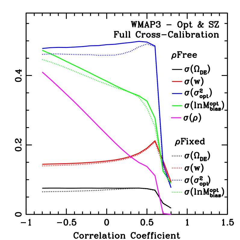
In the right plot, we see that for the cross-calibration using only clusters detected by both methods (i.e. the partial cross-calibration) the constraints are more dependent on the value of the correlation and on its uncertainty. The relation between $\rho$ and the optical bias is most pronounced. As mentioned in the discussion following Eq. (11), variations in the correlation change the distribution of number counts in $M^{\rm obs}_{a}-M^{\rm obs}_{b}$ space in ways that mimic bias and scatter in the observables. In the full cross-calibration, the relation between $\sigma(\rho)$ and $\sigma(lnM^{\rm bias}_{\rm opt})$ is less pronounced because the information from clusters detected only by optical (or SZ) helps to break the degeneracy between the correlation and the bias. Though not shown, the uncertainty in the bias and scatter of the SZ observable scales very similarly to that of the corresponding optical nuisance parameters.

Figure 9: $1-\sigma$ constraints on dark energy and optical-mass nuisance parameters as a function of correlation $\rho$ for (left) the full cross-calibration and (right) the partial cross-calibration. For the solid lines $\rho$ is a free parameter whereas the dotted lines are for $\rho$ fixed. Both plots are for a WMAP3 cosmology.

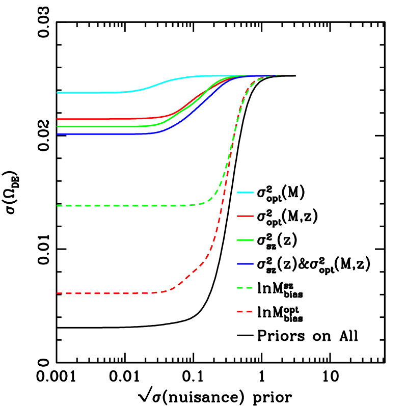
In Figure 10 we show $\sigma(\Omega_{DE})$ (left) and $\sigma(w)$ (right) as functions of the prior on the nuisance parameters for the full calibration analysis. Throughout we assume that $\sigma_{\rm prior}=\sigma_{\rm prior}(\sigma^{2}_{0})=\sigma_{\rm prior}(\ln M^{\rm bias}_{0})=0.5\sigma_{\rm prior}(a_{i})=0.5\sigma_{\rm prior}(b_{i})=0.5\sigma_{\rm prior}(c_{i})$. We see from the left plot that constraints on $\Omega_{\rm DE}$ are most sensitive to priors on the mass bias, especially the optical mass bias. A prior of $(0.1)^{2}$ on ${\ln M^{\rm bias}_{\rm opt}}$ improves $\sigma(\Omega_{\rm DE})$ by a factor of $\sim 3$. With priors of $(0.1)^{2}$ on all parameters (multiplied by two where appropriate) $\sigma(\Omega_{\rm DE})$ improves by approximately an order of magnitude!

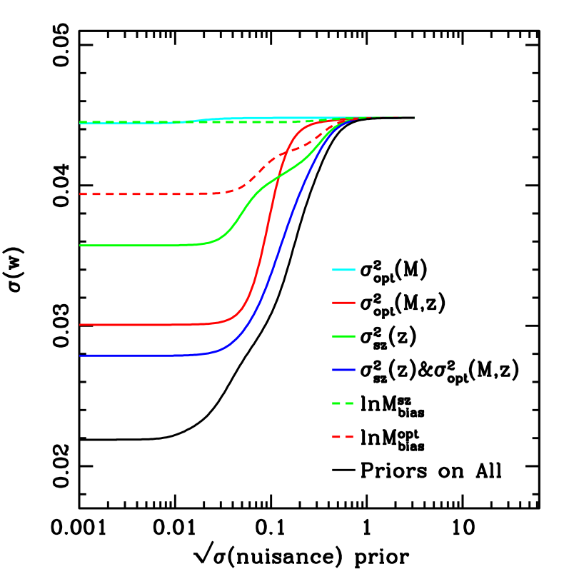
Constraints on $w$ are largely insensitive to priors on the mass-dependent part of the optical scatter, $\sigma^{2}_{opt}(M)$, or on the SZ mass bias parameters. Priors on the optical mass bias improve constraints by at most $12\%$. The constraints are most sensitive to priors on the redshift dependent scatter nuisance parameters, particularly the optical scatter. A prior of $(0.1)^{2}$ on $\sigma^{2}_{opt}(M,z)$ and $\sigma^{2}_{SZ}(z)$ decreases $\sigma(w)$ by a factor of $\sim 1.3$. The full cross-calibration can constrain the constant parts of both the SZ and optical scatter so that priors on them do not improve $w$ constraints. The full improvement requires priors of $(0.01)^{2}$ on all parameters and yields $\sigma(w)=0.022$.

Figure 10: $\sigma(\Omega_{DE})$(left) and $\sigma(w)$ (right) versus the prior on the nuisance parameters for the full calibration analysis. For the cyan lines, priors were applied on the mass dependent part of $\sigma^{2}_{\rm opt}$ only. For the solid red lines priors were applied on all parameters of $\sigma^{2}_{\rm opt}$. Applying priors to all terms of $\sigma^{2}_{\rm sz}$ yields the solid green lines. The blue lines were generated using priors on $\sigma^{2}_{\rm opt}$ and $\sigma^{2}_{\rm sz}$. The dashed green lines have priors on ${\ln M^{\rm bias}_{\rm sz}}$ and the dashed red lines have priors on ${\ln M^{\rm bias}_{\rm opt}}$. Applying priors to all nuisance parameters yields the black lines.

V Conclusions and future work

We developed a formalism to derive joint cosmological and cluster mass-observable constraints from cluster number counts and clustering sample variance of multiple cluster finding techniques. The improvement we find relative to previous works arises from our use of the interdependence of cluster measurements performed over the same patch of sky to cross-calibrate the mass-observable relations of the different techniques. When combining an SPT-like and DES-like survey, the full cross-calibration method yields $\sim 2$ times smaller constraints on $\Omega_{\rm DE}$ and $w$ compared to simply adding the Fisher matrices of the individual experiments. Furthermore, constraints from the full cross-calibration are less sensitive to $M^{\rm th}$ and $z_{\rm max}$ than the single mass-observable constraints.

The cross-calibration places tight constraints on the correlation between the observables without the need of additional priors. Conversely, priors on the mass-variance and bias can significantly improve the dark energy constraints. Constraints on $\Omega_{\rm DE}$ are most sensitive to priors on the mass biases. On the other hand, constraints on $w$ are more sensitive to priors on the redshift-dependent part of the scatters. Priors on the optical nuisance parameters are more relevant than priors on SZ nuisance parameters for both $\Omega_{\rm DE}$ and $w$ constraints.

Our technique can still be improved. Combining more than two techniques at a time should further improve constraints. But we can only combine multiple techniques if we use a more efficient binning strategy, to minimizes the number of mass bins needed to extract the useful information. It is possible that a more efficient binning may improve even the two observable case, particularly in cosmologies with low $\sigma_{8}$.

Work still needs to be done before the self-calibration or full cross-calibration can be applied to real data. The cross-calibration estimates presented here are sensitive to the parametrization of the mass errors. Simulations are needed to determine what parametrizations are robust to theoretical and experimental uncertainties. Our results assumed a perfect selection, but selection effects may bias the cosmological constraints. Wu et al. (2008) have shown that if the halo selection depends on halo concentration, and if the halo bias depends on the assembly history, the sample variance due to clustering will deviate from that of a random selection of halos with the same mass distribution. If the clustering sample variance is modeled incorrectly, the self-calibration may bias the recovered dark energy parameters. Since the different cluster surveys are expected to have selections with different dependence on the halo concentration, cross-calibration should mitigate selection effects, though we are yet to test this hypothesis. Finally, we must still account for the relation between photo-z and mass-observable errors. Regardless of the simplifications adopted here, we conclude that having overlap between surveys is very important to maximize the effectiveness of cross-calibration techniques.

Appendix A The probability distribution of multiple observables

Studies of the cluster mass-observable relation in the literature (e.g. Rykoff et al. (2008b); Johnston et al. (2007); Reyes et al. (2008)), using either simulations or observations, typically estimate $p({M^{\rm obs}}|M)$ (by measuring the scatter of $M^{\rm obs}(M)$) for a single mass-observable or the relation between two observables, $p({M^{\rm obs}}_{a}|M^{\rm obs}_{b})$, for a given $M$, or equivalently, assuming no evolution in $M$. Thus, it is useful to express $p({\bf M^{\rm obs}}|M)$ in terms of combinations of $p({M^{\rm obs}}|M)$ and $p({M^{\rm obs}}_{a}|M^{\rm obs}_{b})$. This can be done using the product rule of probability and Bayes’ theorem. For example, for two observables,

$$p({\bf M^{\rm obs}}|M) = p(M^{\rm obs}_{a},M^{\rm obs}_{b}|M)$$

$$=$$

References

- The Dark Energy Survey Collaboration (2005) The Dark Energy Survey Collaboration, ArXiv Astrophysics e-prints (2005), eprint astro-ph/0510346.
- Tyson and Wolff (2002) J. A. Tyson and S. Wolff, eds., Survey and Other Telescope Technologies and Discoveries, vol. 4836 of Presented at the Society of Photo-Optical Instrumentation Engineers (SPIE) Conference (2002).
- Ruhl et al. (2004) J. Ruhl et al., in Proceedings of the SPIE (2004), vol. 5498, pp. 11–29.
- Kosowsky (2003) A. Kosowsky, New Astronomy Review 47, 939 (2003), eprint arXiv:astro-ph/0402234.
- Predehl et al. (2007) P. Predehl et al., in UV, X-Ray, and Gamma-Ray Space Instrumentation for Astronomy XV. Edited by Siegmund, Oswald H. Proceedings of the SPIE, Volume 6686, pp. 668617-668617-9 (2007). (2007), vol. 6686 of Presented at the Society of Photo-Optical Instrumentation Engineers (SPIE) Conference.
- Majumdar and Mohr (2004) S. Majumdar and J. J. Mohr, Astrophys. J. 613, 41 (2004), eprint arXiv:astro-ph/0305341.
- Lima and Hu (2004) M. Lima and W. Hu, Phys. Rev. D 70, 043504 (2004), eprint arXiv:astro-ph/0401559.
- Lima and Hu (2005) M. Lima and W. Hu, Phys. Rev. D 72, 043006 (2005), eprint arXiv:astro-ph/0503363.
- Hu and Kravtsov (2003) W. Hu and A. V. Kravtsov, Astrophys. J. 584, 702 (2003), eprint arXiv:astro-ph/0203169.
- Rozo et al. (2007) E. Rozo, R. H. Wechsler, B. P. Koester, A. E. Evrard, and T. A. McKay, ArXiv Astrophysics e-prints (2007), eprint arXiv:astro-ph/0703574.
- Levine et al. (2002) E. S. Levine, A. E. Schulz, and M. White, Astrophys. J. 577, 569 (2002), eprint arXiv:astro-ph/0204273.
- Majumdar and Mohr (2003) S. Majumdar and J. J. Mohr, Astrophys. J. 585, 603 (2003), eprint arXiv:astro-ph/0208002.
- Younger et al. (2006) J. D. Younger, Z. Haiman, G. L. Bryan, and S. Wang, Astrophys. J. 653, 27 (2006), eprint arXiv:astro-ph/0605204.
- Jenkins et al. (2001) A. Jenkins, C. S. Frenk, S. D. M. White, J. M. Colberg, S. Cole, A. E. Evrard, H. M. P. Couchman, and N. Yoshida, Mon. Not. R. Astron. Soc. 321, 372 (2001), eprint arXiv:astro-ph/0005260.
- Tinker et al. (2008) J. L. Tinker, A. V. Kravtsov, A. Klypin, K. Abazajian, M. S. Warren, G. Yepes, S. Gottlober, and D. E. Holz, ArXiv e-prints 803 (2008), eprint 0803.2706.
- Warren et al. (2006) M. S. Warren, K. Abazajian, D. E. Holz, and L. Teodoro, Astrophys. J. 646, 881 (2006), eprint arXiv:astro-ph/0506395.
- Lima and Hu (2007) M. Lima and W. Hu, Phys. Rev. D 76, 123013 (2007), eprint arXiv:0709.2871.
- Shaw et al. (2007) L. D. Shaw, G. P. Holder, and P. Bode, ArXiv e-prints 710 (2007), eprint 0710.4555.
- Kravtsov et al. (2006) A. V. Kravtsov, A. Vikhlinin, and D. Nagai, Astrophys. J. 650, 128 (2006), eprint arXiv:astro-ph/0603205.
- Rykoff et al. (2008a) E. S. Rykoff, A. E. Evrard, T. A. McKay, M. R. Becker, D. E. Johnston, B. P. Koester, B. Nord, E. Rozo, E. S. Sheldon, R. Stanek, et al., Mon. Not. R. Astron. Soc. 387, L28 (2008a), eprint arXiv:0802.1069.
- Evrard et al. (2008) A. E. Evrard, J. Bialek, M. Busha, M. White, S. Habib, K. Heitmann, M. Warren, E. Rasia, G. Tormen, L. Moscardini, et al., Astrophys. J. 672, 122 (2008), eprint arXiv:astro-ph/0702241.
- Rykoff et al. (2008b) E. S. Rykoff, T. A. McKay, M. R. Becker, A. Evrard, D. E. Johnston, B. P. Koester, E. Rozo, E. S. Sheldon, and R. H. Wechsler, Astrophys. J. 675, 1106 (2008b), eprint arXiv:0709.1158.
- Cohn et al. (2007) J. D. Cohn, A. E. Evrard, M. White, D. Croton, and E. Ellingson, Red sequence cluster finding in the millennium simulation (2007), URL http://www.citebase.org/abstract?id=oai:arXiv.org:0706.0211.
- Sheth and Tormen (1999) R. K. Sheth and G. Tormen, Mon. Not. R. Astron. Soc. 308, 119 (1999), eprint arXiv:astro-ph/9901122.
- Hu and Cohn (2006) W. Hu and J. D. Cohn, Phys. Rev. D 73, 067301 (2006), eprint arXiv:astro-ph/0602147.
- Holder et al. (2001) G. Holder, Z. Haiman, and J. J. Mohr, Astrophys. J. Lett. 560, L111 (2001), eprint arXiv:astro-ph/0105396.
- Bennett et al. (2003) C. L. Bennett et al., Astrophys. J. Supp. 148, 1 (2003), eprint arXiv:astro-ph/0302207.
- Spergel et al. (2007) D. N. Spergel et al., Astrophys. J. Supp. 170, 377 (2007), eprint arXiv:astro-ph/0603449.
- Seljak and Zaldarriaga (1996) U. Seljak and M. Zaldarriaga, Astrophys. J. 469, 437 (1996), eprint arXiv:astro-ph/9603033.
- Carlstrom et al. (2002) J. E. Carlstrom, G. P. Holder, and E. D. Reese, Annu. Rev. Astron. Astrophys. 40, 643 (2002), eprint arXiv:astro-ph/0208192.
- York (2000) D. G. York, Astronomical Journal 120, 1579 (2000), URL http://www.citebase.org/abstract?id=oai:arXiv.org:astro-ph/00%06396.
- Koester et al. (2007) B. P. Koester, T. A. McKay, J. Annis, R. H. Wechsler, A. Evrard, L. Bleem, M. Becker, D. Johnston, E. Sheldon, R. Nichol, et al., Astrophys. J. 660, 239 (2007), eprint arXiv:astro-ph/0701265.
- Johnston et al. (2007) D. E. Johnston, E. S. Sheldon, R. H. Wechsler, E. Rozo, B. P. Koester, J. A. Frieman, T. A. McKay, A. E. Evrard, M. R. Becker, and J. Annis, ArXiv e-prints 709 (2007), eprint 0709.1159.
- Gladders and Yee (2000) M. D. Gladders and H. K. C. Yee, Astron. J. 120, 2148 (2000), eprint arXiv:astro-ph/0004092.
- Wu et al. (2008) H.-Y. Wu, E. Rozo, and R. H. Wechsler, ArXiv e-prints 803 (2008), eprint 0803.1491.
- Becker et al. (2007) M. R. Becker, T. A. McKay, B. Koester, R. H. Wechsler, E. Rozo, A. Evrard, D. Johnston, E. Sheldon, J. Annis, E. Lau, et al., Astrophys. J. 669, 905 (2007), eprint arXiv:0704.3614.
- Rozo et al. (2008a) E. Rozo, E. S. Rykoff, A. Evrard, M. Becker, T. McKay, R. H. Wechsler, B. P. Koester, J. Hao, S. Hansen, E. Sheldon, et al., Constraining the scatter in the mass-richness relation of maxbcg clusters with weak lensing and x-ray data (2008a), URL http://www.citebase.org/abstract?id=oai:arXiv.org:0809.2794.
- Rozo et al. (2008b) E. Rozo, E. S. Rykoff, B. P. Koester, T. McKay, J. Hao, A. Evrard, R. H. Wechsler, S. Hansen, E. Sheldon, D. Johnston, et al., An improved cluster richness estimator (2008b), URL http://www.citebase.org/abstract?id=oai:arXiv.org:0809.2797.
- Reyes et al. (2008) R. Reyes, R. Mandelbaum, C. M. Hirata, N. Bahcall, and U. Seljak, ArXiv e-prints 802 (2008), eprint 0802.2365.