NLO Higgs boson production via gluon fusion
matched with shower in POWHEG

Simone Alioli
Università di Milano-Bicocca and INFN, Sezione di Milano-Bicocca
Piazza della Scienza 3, 20126 Milan, Italy
E-mail
Simone.Alioli@mib.infn.it
   Paolo Nason
INFN, Sezione di Milano-Bicocca, Piazza della Scienza 3, 20126 Milan, Italy
E-mail
Paolo.Nason@mib.infn.it
   Carlo Oleari
Università di Milano-Bicocca and INFN, Sezione di Milano-Bicocca
Piazza della Scienza 3, 20126 Milan, Italy
E-mail
Carlo.Oleari@mib.infn.it
   Emanuele Re
Università di Milano-Bicocca and INFN, Sezione di Milano-Bicocca
Piazza della Scienza 3, 20126 Milan, Italy
E-mail
Emanuele.Re@mib.infn.it
Abstract:

We present a next-to-leading order calculation of Higgs boson production via gluon fusion interfaced to shower Monte Carlo programs, implemented according to the POWHEG method. A detailed comparison with MC@NLO and PYTHIA is carried out for several observables, for the Tevatron and LHC colliders. Comparisons with next-to-next-to-leading order results and with resummed ones are also presented.

QCD, Monte Carlo, NLO Computations, Resummation, Collider Physics

1 Introduction

Gluon fusion is the dominant Higgs boson production mechanism both at the Tevatron and at the LHC. Radiative corrections to this process are known to be large [1, 2, 3], and it is thus important that shower generators that do include them are made available to the experimental collaborations. In fact, one such generator already exists, namely the MC@NLO implementation [4] of Higgs boson production.

In this work we present a next-to-leading order (NLO) calculation of Higgs boson production via gluon fusion, interfaced to shower Monte Carlo programs according to the POWHEG method. Unlike the MC@NLO implementation, our generator produces events with positive (constant) weight, and, furthermore, is not tied to the HERWIG shower Monte Carlo program. It can be easily interfaced to any modern shower generator and, in fact, we show results of POWHEG interfaced to HERWIG [5, 6] and to PYTHIA [7].

The POWHEG method was first suggested in ref. [8]. In ref. [9] a detailed general description of its application to collider processes was given. Until now, the POWHEG method has been applied to ZZ𝑍𝑍ZZ pair hadroproduction [10], heavy-flavour production [11], e+esuperscript𝑒superscript𝑒e^{+}e^{-} annihilation into hadrons [12] and into top pairs [13], and Drell-Yan vector boson production [14, 15]. We have built our implementation of the Higgs boson production by following closely the formulae and results of ref. [9].

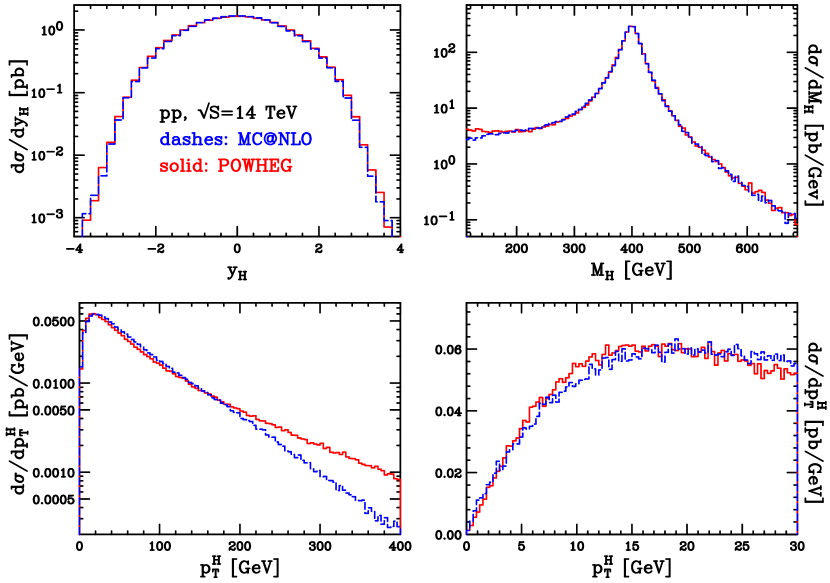
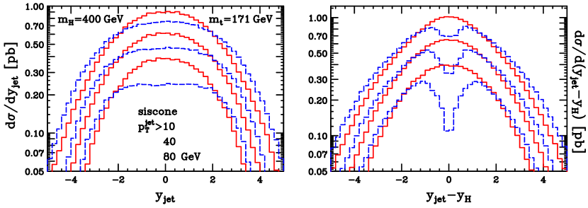
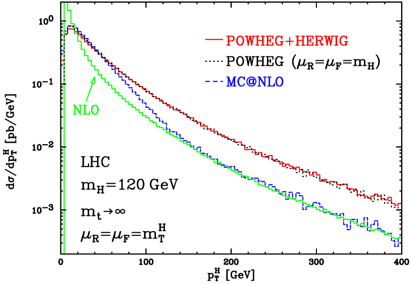
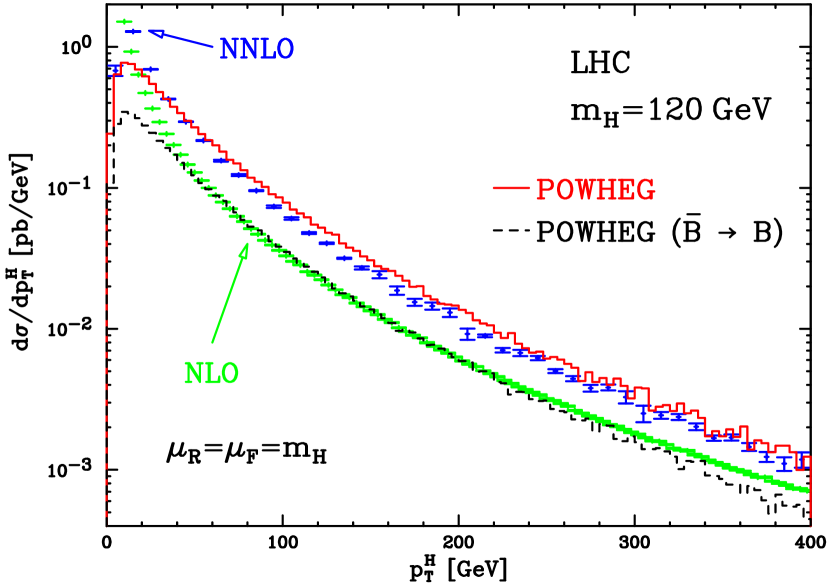
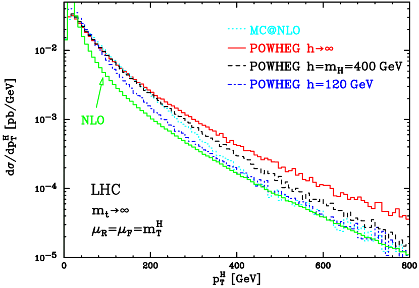
Much of our phenomenological section will be devoted to study the comparison of our result with that of MC@NLO. We find fair agreement between MC@NLO and POWHEG results, except for the pTsubscript𝑝Tp_{\mathchoice{\displaystyle}{\scriptstyle}{\scriptscriptstyle}{\scriptscriptstyle}\rm T} distribution of the Higgs boson, and consequently of the hardest jet, in the high-pTsubscript𝑝Tp_{\mathchoice{\displaystyle}{\scriptstyle}{\scriptscriptstyle}{\scriptscriptstyle}\rm T} region. In this region, the POWHEG distributions are generally harder. We have shown that this is due to next-to-next-to-leading order (NNLO) effects in the POWHEG formula for the differential cross section. We checked that these effects actually bring our result closer to the NNLO one [16]. Other relevant discrepancies are found in the rapidity difference of the Higgs boson and the hardest jet. The dip produced by the MC@NLO program, found in previous implementations [10, 11, 14], is present also here. We remark that this seems to be a general feature of MC@NLO, since other calculations do not find effects of this kind [17, 18, 19].

The paper is organized as follows. In sec. 2 we describe how we performed the calculation for the Higgs boson cross section at the next-to-leading order. In sec. 3 we discuss the POWHEG implementation. In sec. 4 we show our results for several kinematic variables and compare them with the MC@NLO [4] and PYTHIA 6.4 [7] shower Monte Carlo programs. A comparison with next-to-next-to-leading order results, as well as with analytical resummed ones is also carried out. In sec. 5, we give our conclusions.

2 Description of the calculation

In this section we fix our kinematic notation, and give the Higgs boson production differential cross sections up to next-to-leading order in the strong coupling αSsubscript𝛼S\alpha_{\mathchoice{\displaystyle}{\scriptstyle}{\scriptscriptstyle}{\scriptscriptstyle}\rm S}.

2.1 Kinematics

2.1.1 Born kinematics

The Born process has a single partonic contribution, ggH𝑔𝑔𝐻gg\to H. Following the notation of ref. [9], we denote with k¯subscript¯𝑘direct-sum\bar{k}_{{\mathchoice{\displaystyle}{\scriptstyle}{\scriptscriptstyle}{\scriptscriptstyle}\oplus}} and k¯subscript¯𝑘symmetric-difference\bar{k}_{{\mathchoice{\displaystyle}{\scriptstyle}{\scriptscriptstyle}{\scriptscriptstyle}\ominus}} the incoming gluon momenta, aligned along the plus and minus direction of the z𝑧z axis, and by k¯1subscript¯𝑘1\bar{k}_{1} the outgoing Higgs boson momentum. If Ksubscript𝐾direct-sumK_{\mathchoice{\displaystyle}{\scriptstyle}{\scriptscriptstyle}{\scriptscriptstyle}\oplus} and Ksubscript𝐾symmetric-differenceK_{\mathchoice{\displaystyle}{\scriptstyle}{\scriptscriptstyle}{\scriptscriptstyle}\ominus} are the momenta of the incoming hadrons, then we have

k¯   =x¯   K   ,subscript¯𝑘   subscript¯𝑥   subscript𝐾   \bar{k}_{\mathchoice{\makebox[8.55556pt]{\makebox[0.0pt]{\rule[1.9444pt]{4.27777pt}{0.24306pt}}\makebox[0.0pt]{\rule[0.48613pt]{4.27777pt}{0.24306pt}}\makebox[0.0pt]{\rule[0.48613pt]{0.4278pt}{2.91669pt}}\makebox[0.0pt]{$\displaystyle\bigcirc$}}}{\makebox[6.45555pt]{\makebox[0.0pt]{\rule[1.36108pt]{3.22777pt}{0.17014pt}}\makebox[0.0pt]{\rule[0.34029pt]{3.22777pt}{0.17014pt}}\makebox[0.0pt]{\rule[0.34029pt]{0.32278pt}{2.04167pt}}\makebox[0.0pt]{$\scriptstyle\bigcirc$}}}{\makebox[5.05554pt]{\makebox[0.0pt]{\rule[0.9722pt]{2.52777pt}{0.12152pt}}\makebox[0.0pt]{\rule[0.24306pt]{2.52777pt}{0.12152pt}}\makebox[0.0pt]{\rule[0.24306pt]{0.25279pt}{1.45833pt}}\makebox[0.0pt]{$\scriptscriptstyle\bigcirc$}}}{\makebox[5.05554pt]{\makebox[0.0pt]{\rule[0.9722pt]{2.52777pt}{0.12152pt}}\makebox[0.0pt]{\rule[0.24306pt]{2.52777pt}{0.12152pt}}\makebox[0.0pt]{\rule[0.24306pt]{0.25279pt}{1.45833pt}}\makebox[0.0pt]{$\scriptscriptstyle\bigcirc$}}}}=\bar{x}_{\mathchoice{\makebox[8.55556pt]{\makebox[0.0pt]{\rule[1.9444pt]{4.27777pt}{0.24306pt}}\makebox[0.0pt]{\rule[0.48613pt]{4.27777pt}{0.24306pt}}\makebox[0.0pt]{\rule[0.48613pt]{0.4278pt}{2.91669pt}}\makebox[0.0pt]{$\displaystyle\bigcirc$}}}{\makebox[6.45555pt]{\makebox[0.0pt]{\rule[1.36108pt]{3.22777pt}{0.17014pt}}\makebox[0.0pt]{\rule[0.34029pt]{3.22777pt}{0.17014pt}}\makebox[0.0pt]{\rule[0.34029pt]{0.32278pt}{2.04167pt}}\makebox[0.0pt]{$\scriptstyle\bigcirc$}}}{\makebox[5.05554pt]{\makebox[0.0pt]{\rule[0.9722pt]{2.52777pt}{0.12152pt}}\makebox[0.0pt]{\rule[0.24306pt]{2.52777pt}{0.12152pt}}\makebox[0.0pt]{\rule[0.24306pt]{0.25279pt}{1.45833pt}}\makebox[0.0pt]{$\scriptscriptstyle\bigcirc$}}}{\makebox[5.05554pt]{\makebox[0.0pt]{\rule[0.9722pt]{2.52777pt}{0.12152pt}}\makebox[0.0pt]{\rule[0.24306pt]{2.52777pt}{0.12152pt}}\makebox[0.0pt]{\rule[0.24306pt]{0.25279pt}{1.45833pt}}\makebox[0.0pt]{$\scriptscriptstyle\bigcirc$}}}}K_{\mathchoice{\makebox[8.55556pt]{\makebox[0.0pt]{\rule[1.9444pt]{4.27777pt}{0.24306pt}}\makebox[0.0pt]{\rule[0.48613pt]{4.27777pt}{0.24306pt}}\makebox[0.0pt]{\rule[0.48613pt]{0.4278pt}{2.91669pt}}\makebox[0.0pt]{$\displaystyle\bigcirc$}}}{\makebox[6.45555pt]{\makebox[0.0pt]{\rule[1.36108pt]{3.22777pt}{0.17014pt}}\makebox[0.0pt]{\rule[0.34029pt]{3.22777pt}{0.17014pt}}\makebox[0.0pt]{\rule[0.34029pt]{0.32278pt}{2.04167pt}}\makebox[0.0pt]{$\scriptstyle\bigcirc$}}}{\makebox[5.05554pt]{\makebox[0.0pt]{\rule[0.9722pt]{2.52777pt}{0.12152pt}}\makebox[0.0pt]{\rule[0.24306pt]{2.52777pt}{0.12152pt}}\makebox[0.0pt]{\rule[0.24306pt]{0.25279pt}{1.45833pt}}\makebox[0.0pt]{$\scriptscriptstyle\bigcirc$}}}{\makebox[5.05554pt]{\makebox[0.0pt]{\rule[0.9722pt]{2.52777pt}{0.12152pt}}\makebox[0.0pt]{\rule[0.24306pt]{2.52777pt}{0.12152pt}}\makebox[0.0pt]{\rule[0.24306pt]{0.25279pt}{1.45833pt}}\makebox[0.0pt]{$\scriptscriptstyle\bigcirc$}}}}\,, (1)

where x¯   subscript¯𝑥   \bar{x}_{\mathchoice{\makebox[8.55556pt]{\makebox[0.0pt]{\rule[1.9444pt]{4.27777pt}{0.24306pt}}\makebox[0.0pt]{\rule[0.48613pt]{4.27777pt}{0.24306pt}}\makebox[0.0pt]{\rule[0.48613pt]{0.4278pt}{2.91669pt}}\makebox[0.0pt]{$\displaystyle\bigcirc$}}}{\makebox[6.45555pt]{\makebox[0.0pt]{\rule[1.36108pt]{3.22777pt}{0.17014pt}}\makebox[0.0pt]{\rule[0.34029pt]{3.22777pt}{0.17014pt}}\makebox[0.0pt]{\rule[0.34029pt]{0.32278pt}{2.04167pt}}\makebox[0.0pt]{$\scriptstyle\bigcirc$}}}{\makebox[5.05554pt]{\makebox[0.0pt]{\rule[0.9722pt]{2.52777pt}{0.12152pt}}\makebox[0.0pt]{\rule[0.24306pt]{2.52777pt}{0.12152pt}}\makebox[0.0pt]{\rule[0.24306pt]{0.25279pt}{1.45833pt}}\makebox[0.0pt]{$\scriptscriptstyle\bigcirc$}}}{\makebox[5.05554pt]{\makebox[0.0pt]{\rule[0.9722pt]{2.52777pt}{0.12152pt}}\makebox[0.0pt]{\rule[0.24306pt]{2.52777pt}{0.12152pt}}\makebox[0.0pt]{\rule[0.24306pt]{0.25279pt}{1.45833pt}}\makebox[0.0pt]{$\scriptscriptstyle\bigcirc$}}}} are the momentum fractions, and momentum conservation reads

k¯+k¯=k¯1.subscript¯𝑘direct-sumsubscript¯𝑘symmetric-differencesubscript¯𝑘1\bar{k}_{\mathchoice{\displaystyle}{\scriptstyle}{\scriptscriptstyle}{\scriptscriptstyle}\oplus}+\bar{k}_{\mathchoice{\displaystyle}{\scriptstyle}{\scriptscriptstyle}{\scriptscriptstyle}\ominus}=\bar{k}_{1}\,. (2)

We introduce the Higgs boson invariant mass squared and rapidity

M2=k¯12,Y=12logk¯10+k¯13k¯10k¯13,formulae-sequencesuperscript𝑀2superscriptsubscript¯𝑘12𝑌12superscriptsubscript¯𝑘10superscriptsubscript¯𝑘13superscriptsubscript¯𝑘10superscriptsubscript¯𝑘13M^{2}=\bar{k}_{1}^{2},\qquad\quad Y=\frac{1}{2}\log\frac{\bar{k}_{1}^{0}+\bar{k}_{1}^{3}}{\bar{k}_{1}^{0}-\bar{k}_{1}^{3}}\,, (3)

so that the set of variables 𝚽¯1{M2,Y}subscript¯𝚽1superscript𝑀2𝑌{\bf\bar{\Phi}}_{1}\equiv\left\{M^{2},Y\right\} fully parametrizes the Born kinematics. From them, we can reconstruct the momentum fractions

x¯=M2SeY,x¯=M2SeY,formulae-sequencesubscript¯𝑥direct-sumsuperscript𝑀2𝑆superscript𝑒𝑌subscript¯𝑥symmetric-differencesuperscript𝑀2𝑆superscript𝑒𝑌\bar{x}_{{\mathchoice{\displaystyle}{\scriptstyle}{\scriptscriptstyle}{\scriptscriptstyle}\oplus}}=\sqrt{\frac{M^{2}}{S}}e^{Y},\qquad\quad\bar{x}_{{\mathchoice{\displaystyle}{\scriptstyle}{\scriptscriptstyle}{\scriptscriptstyle}\ominus}}=\sqrt{\frac{M^{2}}{S}}e^{-Y}, (4)

where S=(K+K)2𝑆superscriptsubscript𝐾direct-sumsubscript𝐾symmetric-difference2S=(K_{\mathchoice{\displaystyle}{\scriptstyle}{\scriptscriptstyle}{\scriptscriptstyle}\oplus}+K_{\mathchoice{\displaystyle}{\scriptstyle}{\scriptscriptstyle}{\scriptscriptstyle}\ominus})^{2} is the squared center-of-mass energy of the hadronic collider. The Born phase space, in terms of these variables, can be written as

d𝚽¯1=dx¯dx¯(2π)4δ4(k¯+k¯k¯1)d3k¯1(2π)32k¯10=2πSδ(M2mH2)dM2dY.𝑑subscript¯𝚽1𝑑subscript¯𝑥direct-sum𝑑subscript¯𝑥symmetric-differencesuperscript2𝜋4superscript𝛿4subscript¯𝑘direct-sumsubscript¯𝑘symmetric-differencesubscript¯𝑘1superscript𝑑3subscript¯𝑘1superscript2𝜋32superscriptsubscript¯𝑘102𝜋𝑆𝛿superscript𝑀2superscriptsubscript𝑚𝐻2𝑑superscript𝑀2𝑑𝑌d{\bf\bar{\Phi}}_{1}=d\bar{x}_{\mathchoice{\displaystyle}{\scriptstyle}{\scriptscriptstyle}{\scriptscriptstyle}\oplus}\,d\bar{x}_{\mathchoice{\displaystyle}{\scriptstyle}{\scriptscriptstyle}{\scriptscriptstyle}\ominus}(2\pi)^{4}\delta^{4}(\bar{k}_{\mathchoice{\displaystyle}{\scriptstyle}{\scriptscriptstyle}{\scriptscriptstyle}\oplus}+\bar{k}_{\mathchoice{\displaystyle}{\scriptstyle}{\scriptscriptstyle}{\scriptscriptstyle}\ominus}-\bar{k}_{1})\frac{d^{3}\bar{k}_{1}}{(2\pi)^{3}2\bar{k}_{1}^{0}}\,=\frac{2\pi}{S}\delta\!\left(M^{2}-m_{H}^{2}\right)dM^{2}\,dY\,. (5)

We generate the Higgs boson virtuality according to a Breit-Wigner distribution, i.e. we make the replacement111In order to compare our result with other programs, we have also used slightly different forms of the Breit-Wigner distribution, that will be illustrated in due time.

δ(M2mH2)1πM2ΓH/mH(M2mH2)2+(M2ΓH/mH)2.𝛿superscript𝑀2superscriptsubscript𝑚𝐻21𝜋superscript𝑀2subscriptΓ𝐻subscript𝑚𝐻superscriptsuperscript𝑀2superscriptsubscript𝑚𝐻22superscriptsuperscript𝑀2subscriptΓ𝐻subscript𝑚𝐻2\delta\!\left(M^{2}-m_{H}^{2}\right)\,\to\,\frac{1}{\pi}\frac{M^{2}\,\Gamma_{H}/m_{H}}{\left(M^{2}-m_{H}^{2}\right)^{2}+(M^{2}\,\Gamma_{H}/m_{H})^{2}}. (6)

The decay of the Higgs boson is left to the shower Monte Carlo program, since, being the Higgs boson a scalar, no spin correlation can arise.

2.1.2 Real-emission kinematics

The real emission processes have an additional final-state parton, so that momentum conservation reads

k+k=k1+k2,subscript𝑘direct-sumsubscript𝑘symmetric-differencesubscript𝑘1subscript𝑘2k_{\mathchoice{\displaystyle}{\scriptstyle}{\scriptscriptstyle}{\scriptscriptstyle}\oplus}+k_{\mathchoice{\displaystyle}{\scriptstyle}{\scriptscriptstyle}{\scriptscriptstyle}\ominus}=k_{1}+k_{2}\,, (7)

where k1subscript𝑘1k_{1} is the Higgs boson momentum and k2subscript𝑘2k_{2} is the momentum of the additional final-state parton in the laboratory frame and

k   =x   K   .subscript𝑘   subscript𝑥   subscript𝐾   k_{\mathchoice{\makebox[8.55556pt]{\makebox[0.0pt]{\rule[1.9444pt]{4.27777pt}{0.24306pt}}\makebox[0.0pt]{\rule[0.48613pt]{4.27777pt}{0.24306pt}}\makebox[0.0pt]{\rule[0.48613pt]{0.4278pt}{2.91669pt}}\makebox[0.0pt]{$\displaystyle\bigcirc$}}}{\makebox[6.45555pt]{\makebox[0.0pt]{\rule[1.36108pt]{3.22777pt}{0.17014pt}}\makebox[0.0pt]{\rule[0.34029pt]{3.22777pt}{0.17014pt}}\makebox[0.0pt]{\rule[0.34029pt]{0.32278pt}{2.04167pt}}\makebox[0.0pt]{$\scriptstyle\bigcirc$}}}{\makebox[5.05554pt]{\makebox[0.0pt]{\rule[0.9722pt]{2.52777pt}{0.12152pt}}\makebox[0.0pt]{\rule[0.24306pt]{2.52777pt}{0.12152pt}}\makebox[0.0pt]{\rule[0.24306pt]{0.25279pt}{1.45833pt}}\makebox[0.0pt]{$\scriptscriptstyle\bigcirc$}}}{\makebox[5.05554pt]{\makebox[0.0pt]{\rule[0.9722pt]{2.52777pt}{0.12152pt}}\makebox[0.0pt]{\rule[0.24306pt]{2.52777pt}{0.12152pt}}\makebox[0.0pt]{\rule[0.24306pt]{0.25279pt}{1.45833pt}}\makebox[0.0pt]{$\scriptscriptstyle\bigcirc$}}}}=x_{\mathchoice{\makebox[8.55556pt]{\makebox[0.0pt]{\rule[1.9444pt]{4.27777pt}{0.24306pt}}\makebox[0.0pt]{\rule[0.48613pt]{4.27777pt}{0.24306pt}}\makebox[0.0pt]{\rule[0.48613pt]{0.4278pt}{2.91669pt}}\makebox[0.0pt]{$\displaystyle\bigcirc$}}}{\makebox[6.45555pt]{\makebox[0.0pt]{\rule[1.36108pt]{3.22777pt}{0.17014pt}}\makebox[0.0pt]{\rule[0.34029pt]{3.22777pt}{0.17014pt}}\makebox[0.0pt]{\rule[0.34029pt]{0.32278pt}{2.04167pt}}\makebox[0.0pt]{$\scriptstyle\bigcirc$}}}{\makebox[5.05554pt]{\makebox[0.0pt]{\rule[0.9722pt]{2.52777pt}{0.12152pt}}\makebox[0.0pt]{\rule[0.24306pt]{2.52777pt}{0.12152pt}}\makebox[0.0pt]{\rule[0.24306pt]{0.25279pt}{1.45833pt}}\makebox[0.0pt]{$\scriptscriptstyle\bigcirc$}}}{\makebox[5.05554pt]{\makebox[0.0pt]{\rule[0.9722pt]{2.52777pt}{0.12152pt}}\makebox[0.0pt]{\rule[0.24306pt]{2.52777pt}{0.12152pt}}\makebox[0.0pt]{\rule[0.24306pt]{0.25279pt}{1.45833pt}}\makebox[0.0pt]{$\scriptscriptstyle\bigcirc$}}}}K_{\mathchoice{\makebox[8.55556pt]{\makebox[0.0pt]{\rule[1.9444pt]{4.27777pt}{0.24306pt}}\makebox[0.0pt]{\rule[0.48613pt]{4.27777pt}{0.24306pt}}\makebox[0.0pt]{\rule[0.48613pt]{0.4278pt}{2.91669pt}}\makebox[0.0pt]{$\displaystyle\bigcirc$}}}{\makebox[6.45555pt]{\makebox[0.0pt]{\rule[1.36108pt]{3.22777pt}{0.17014pt}}\makebox[0.0pt]{\rule[0.34029pt]{3.22777pt}{0.17014pt}}\makebox[0.0pt]{\rule[0.34029pt]{0.32278pt}{2.04167pt}}\makebox[0.0pt]{$\scriptstyle\bigcirc$}}}{\makebox[5.05554pt]{\makebox[0.0pt]{\rule[0.9722pt]{2.52777pt}{0.12152pt}}\makebox[0.0pt]{\rule[0.24306pt]{2.52777pt}{0.12152pt}}\makebox[0.0pt]{\rule[0.24306pt]{0.25279pt}{1.45833pt}}\makebox[0.0pt]{$\scriptscriptstyle\bigcirc$}}}{\makebox[5.05554pt]{\makebox[0.0pt]{\rule[0.9722pt]{2.52777pt}{0.12152pt}}\makebox[0.0pt]{\rule[0.24306pt]{2.52777pt}{0.12152pt}}\makebox[0.0pt]{\rule[0.24306pt]{0.25279pt}{1.45833pt}}\makebox[0.0pt]{$\scriptscriptstyle\bigcirc$}}}}\,. (8)

Since we regularize the infrared divergences in the Frixione, Kunszt and Signer (FKS) subtraction scheme [20, 21], we introduce the appropriate set of radiation variables. In the partonic center-of-mass frame, the final-state parton has momentum

k2=k2 0(1,sinθsinϕ,sinθcosϕ,cosθ),subscriptsuperscript𝑘2superscriptsubscript𝑘2 01𝜃italic-ϕ𝜃italic-ϕ𝜃k^{\prime}_{2}=k_{2}^{\prime\,0}\ (1,\sin\theta\sin\phi,\sin\theta\cos\phi,\cos\theta), (9)

and we use the set Φrad{ξ,y,ϕ}subscriptΦrad𝜉𝑦italic-ϕ\Phi_{\rm rad}\equiv\left\{\xi,y,\phi\right\} as radiation variables, where

k2 0=s2ξ,y=cosθ,formulae-sequencesuperscriptsubscript𝑘2 0𝑠2𝜉𝑦𝜃k_{2}^{\prime\,0}=\frac{\sqrt{s}}{2}\xi,\qquad y=\cos\theta\,, (10)

and

s=(k+k)2=M21ξ𝑠superscriptsubscript𝑘direct-sumsubscript𝑘symmetric-difference2superscript𝑀21𝜉s=\left(k_{\mathchoice{\displaystyle}{\scriptstyle}{\scriptscriptstyle}{\scriptscriptstyle}\oplus}+k_{\mathchoice{\displaystyle}{\scriptstyle}{\scriptscriptstyle}{\scriptscriptstyle}\ominus}\right)^{2}=\frac{M^{2}}{1-\xi} (11)

is the partonic center-of-mass energy squared. Since there are no final-state coloured partons at the Born level, we have to deal with initial-state singularities only. The soft singularity is characterized by ξ0𝜉0\xi\to 0, while the collinear limits (k2subscript𝑘2k_{2} parallel to the direct-sum{\mathchoice{\displaystyle}{\scriptstyle}{\scriptscriptstyle}{\scriptscriptstyle}\oplus} or symmetric-difference{\mathchoice{\displaystyle}{\scriptstyle}{\scriptscriptstyle}{\scriptscriptstyle}\ominus} incoming directions) are characterized by y1𝑦1y\to 1 and y1𝑦1y\to-1 respectively.

2.1.3 Inverse construction

The set of variables 𝚽2{M2,Y,ξ,y,ϕ}subscript𝚽2superscript𝑀2𝑌𝜉𝑦italic-ϕ{\bf\Phi}_{2}\equiv\left\{M^{2},Y,\xi,y,\phi\right\} fully specifies the real-emission kinematics. In fact, given these variables, we can reconstruct all the momenta. Using eq. (4), we can compute the underlying Born momentum fractions x¯   subscript¯𝑥   \bar{x}_{\mathchoice{\makebox[8.55556pt]{\makebox[0.0pt]{\rule[1.9444pt]{4.27777pt}{0.24306pt}}\makebox[0.0pt]{\rule[0.48613pt]{4.27777pt}{0.24306pt}}\makebox[0.0pt]{\rule[0.48613pt]{0.4278pt}{2.91669pt}}\makebox[0.0pt]{$\displaystyle\bigcirc$}}}{\makebox[6.45555pt]{\makebox[0.0pt]{\rule[1.36108pt]{3.22777pt}{0.17014pt}}\makebox[0.0pt]{\rule[0.34029pt]{3.22777pt}{0.17014pt}}\makebox[0.0pt]{\rule[0.34029pt]{0.32278pt}{2.04167pt}}\makebox[0.0pt]{$\scriptstyle\bigcirc$}}}{\makebox[5.05554pt]{\makebox[0.0pt]{\rule[0.9722pt]{2.52777pt}{0.12152pt}}\makebox[0.0pt]{\rule[0.24306pt]{2.52777pt}{0.12152pt}}\makebox[0.0pt]{\rule[0.24306pt]{0.25279pt}{1.45833pt}}\makebox[0.0pt]{$\scriptscriptstyle\bigcirc$}}}{\makebox[5.05554pt]{\makebox[0.0pt]{\rule[0.9722pt]{2.52777pt}{0.12152pt}}\makebox[0.0pt]{\rule[0.24306pt]{2.52777pt}{0.12152pt}}\makebox[0.0pt]{\rule[0.24306pt]{0.25279pt}{1.45833pt}}\makebox[0.0pt]{$\scriptscriptstyle\bigcirc$}}}} and, following sec. 5 of ref [9], we have

x=x¯1ξ2ξ(1y)2ξ(1+y),x=x¯1ξ2ξ(1+y)2ξ(1y),formulae-sequencesubscript𝑥direct-sumsubscript¯𝑥direct-sum1𝜉2𝜉1𝑦2𝜉1𝑦subscript𝑥symmetric-differencesubscript¯𝑥symmetric-difference1𝜉2𝜉1𝑦2𝜉1𝑦x_{\mathchoice{\displaystyle}{\scriptstyle}{\scriptscriptstyle}{\scriptscriptstyle}\oplus}=\frac{\bar{x}_{\mathchoice{\displaystyle}{\scriptstyle}{\scriptscriptstyle}{\scriptscriptstyle}\oplus}}{\sqrt{1-\xi}}\sqrt{\frac{2-\xi(1-y)}{2-\xi(1+y)}},\qquad x_{\mathchoice{\displaystyle}{\scriptstyle}{\scriptscriptstyle}{\scriptscriptstyle}\ominus}=\frac{\bar{x}_{\mathchoice{\displaystyle}{\scriptstyle}{\scriptscriptstyle}{\scriptscriptstyle}\ominus}}{\sqrt{1-\xi}}\sqrt{\frac{2-\xi(1+y)}{2-\xi(1-y)}}, (12)

with the kinematics constraints

0ξξM(y),0𝜉subscript𝜉M𝑦0\leq\xi\leq{\xi_{\mathchoice{\displaystyle}{\scriptstyle}{\scriptscriptstyle}{\scriptscriptstyle}\rm{M}}}(y)\ , (13)

where

ξM(y)=1maxsubscript𝜉M𝑦1max\displaystyle{\xi_{\mathchoice{\displaystyle}{\scriptstyle}{\scriptscriptstyle}{\scriptscriptstyle}\rm{M}}}(y)=1-{\rm max}\!\!\! {2(1+y)x¯2(1+x¯2)2(1y)2+16yx¯2+(1y)(1x¯2),\displaystyle\left\{\frac{2(1+y)\,\bar{x}_{\mathchoice{\displaystyle}{\scriptstyle}{\scriptscriptstyle}{\scriptscriptstyle}\oplus}^{2}}{\sqrt{(1+\bar{x}_{\mathchoice{\displaystyle}{\scriptstyle}{\scriptscriptstyle}{\scriptscriptstyle}\oplus}^{2})^{2}(1-y)^{2}+16\,y\,\bar{x}_{\mathchoice{\displaystyle}{\scriptstyle}{\scriptscriptstyle}{\scriptscriptstyle}\oplus}^{2}}+(1-y)(1-\bar{x}_{\mathchoice{\displaystyle}{\scriptstyle}{\scriptscriptstyle}{\scriptscriptstyle}\oplus}^{2})},\right. (14)
2(1y)x¯2(1+x¯2)2(1+y)216yx¯2+(1+y)(1x¯2)}.\displaystyle\phantom{\Bigg{\{}}\left.\frac{2(1-y)\,\bar{x}_{\mathchoice{\displaystyle}{\scriptstyle}{\scriptscriptstyle}{\scriptscriptstyle}\ominus}^{2}}{\sqrt{(1+\bar{x}_{\mathchoice{\displaystyle}{\scriptstyle}{\scriptscriptstyle}{\scriptscriptstyle}\ominus}^{2})^{2}(1+y)^{2}-16\,y\,\bar{x}_{\mathchoice{\displaystyle}{\scriptstyle}{\scriptscriptstyle}{\scriptscriptstyle}\ominus}^{2}}+(1+y)(1-\bar{x}_{\mathchoice{\displaystyle}{\scriptstyle}{\scriptscriptstyle}{\scriptscriptstyle}\ominus}^{2})}\right\}.

The momentum of the final-state parton in the partonic center-of-mass frame is given by eqs. (9) and (10). We then make a longitudinal boost 𝔹Lsubscript𝔹𝐿\mathbb{B}_{L} from the center-of-mass frame back to the laboratory frame, with boost velocity

β=xxx+x,𝛽subscript𝑥direct-sumsubscript𝑥symmetric-differencesubscript𝑥direct-sumsubscript𝑥symmetric-difference\beta=\frac{x_{\mathchoice{\displaystyle}{\scriptstyle}{\scriptscriptstyle}{\scriptscriptstyle}\oplus}-x_{\mathchoice{\displaystyle}{\scriptstyle}{\scriptscriptstyle}{\scriptscriptstyle}\ominus}}{x_{\mathchoice{\displaystyle}{\scriptstyle}{\scriptscriptstyle}{\scriptscriptstyle}\oplus}+x_{\mathchoice{\displaystyle}{\scriptstyle}{\scriptscriptstyle}{\scriptscriptstyle}\ominus}}\,, (15)

to obtain k2subscript𝑘2k_{2} from k2superscriptsubscript𝑘2k_{2}^{\prime}

k2=𝔹Lk2.subscript𝑘2subscript𝔹𝐿superscriptsubscript𝑘2k_{2}=\mathbb{B}_{L}\,k_{2}^{\prime}\,. (16)

From momentum conservation, we reconstruct the Higgs boson momentum

k1=xK+xKk2.subscript𝑘1subscript𝑥direct-sumsubscript𝐾direct-sumsubscript𝑥symmetric-differencesubscript𝐾symmetric-differencesubscript𝑘2k_{1}=x_{\mathchoice{\displaystyle}{\scriptstyle}{\scriptscriptstyle}{\scriptscriptstyle}\oplus}K_{\mathchoice{\displaystyle}{\scriptstyle}{\scriptscriptstyle}{\scriptscriptstyle}\oplus}+x_{\mathchoice{\displaystyle}{\scriptstyle}{\scriptscriptstyle}{\scriptscriptstyle}\ominus}K_{\mathchoice{\displaystyle}{\scriptstyle}{\scriptscriptstyle}{\scriptscriptstyle}\ominus}-k_{2}\,. (17)

Finally, the two-body phase space can be written in a factorized form in terms of the Born and radiation phase space

d𝚽2=dxdx(2π)4δ4(k+kk1k2)d3k1(2π)32k10d3k2(2π)32k20=d𝚽¯1dΦrad,𝑑subscript𝚽2𝑑subscript𝑥direct-sum𝑑subscript𝑥symmetric-differencesuperscript2𝜋4superscript𝛿4subscript𝑘direct-sumsubscript𝑘symmetric-differencesubscript𝑘1subscript𝑘2superscript𝑑3subscript𝑘1superscript2𝜋32superscriptsubscript𝑘10superscript𝑑3subscript𝑘2superscript2𝜋32superscriptsubscript𝑘20𝑑subscript¯𝚽1𝑑subscriptΦradd{\bf\Phi}_{2}=dx_{\mathchoice{\displaystyle}{\scriptstyle}{\scriptscriptstyle}{\scriptscriptstyle}\oplus}\,dx_{\mathchoice{\displaystyle}{\scriptstyle}{\scriptscriptstyle}{\scriptscriptstyle}\ominus}(2\pi)^{4}\delta^{4}(k_{\mathchoice{\displaystyle}{\scriptstyle}{\scriptscriptstyle}{\scriptscriptstyle}\oplus}+k_{\mathchoice{\displaystyle}{\scriptstyle}{\scriptscriptstyle}{\scriptscriptstyle}\ominus}-k_{1}-k_{2})\frac{d^{3}k_{1}}{(2\pi)^{3}2k_{1}^{0}}\frac{d^{3}k_{2}}{(2\pi)^{3}2k_{2}^{0}}=d{\bf\bar{\Phi}}_{1}\,d\Phi_{\rm rad}\,, (18)

where

dΦrad=M2(4π)3ξ(1ξ)2dξdydϕ.𝑑subscriptΦradsuperscript𝑀2superscript4𝜋3𝜉superscript1𝜉2𝑑𝜉𝑑𝑦𝑑italic-ϕd\Phi_{\rm rad}=\frac{M^{2}}{(4\pi)^{3}}\,\frac{\xi}{\left(1-\xi\right)^{2}}\,d\xi\,dy\,d\phi\,. (19)

2.2 Cross sections

In order to apply the POWHEG method, we need the Born, real and virtual contributions to the differential cross section, i.e. the squared amplitudes, averaged over colours and helicities of the incoming partons, and multiplied by the appropriate flux factor.

2.2.1 Born contribution

At Born level, Higgs boson production via gluon fusion proceeds through the coupling of the Higgs boson to a heavy-quark loop. The squared matrix element for the lowest-order contribution, averaged over colours and helicities of the incoming gluons, and multiplied by the flux factor 1/(2M2)12superscript𝑀21/(2M^{2}), is given by

gg=αS2π2GFM25762|32QτQ[1+(1τQ)f(τQ)]|2,subscript𝑔𝑔superscriptsubscript𝛼S2superscript𝜋2subscript𝐺𝐹superscript𝑀25762superscript32subscript𝑄subscript𝜏𝑄delimited-[]11subscript𝜏𝑄𝑓subscript𝜏𝑄2\mathcal{B}_{gg}=\frac{\alpha_{\mathchoice{\displaystyle}{\scriptstyle}{\scriptscriptstyle}{\scriptscriptstyle}\rm S}^{2}}{\pi^{2}}\frac{G_{F}\,M^{2}}{576\,\sqrt{2}}\,\Bigg{|}\,\frac{3}{2}\sum_{Q}\tau_{Q}\Big{[}1+(1-\tau_{Q})f(\tau_{Q})\Big{]}\Bigg{|}^{2}\,, (20)

where τQ=4mQ2/M2subscript𝜏𝑄4subscriptsuperscript𝑚2𝑄superscript𝑀2\tau_{Q}=4m^{2}_{Q}/M^{2}, and the sum runs over the heavy flavours with mass mQsubscript𝑚𝑄m_{Q} circulating in the loop. The function f𝑓f is given by

f(τQ)𝑓subscript𝜏𝑄\displaystyle f(\tau_{Q}) =\displaystyle= {arcsin21τQτQ1,14[log(1+(1τQ)1(1τQ))iπ]2τQ<1.casessuperscript21subscript𝜏𝑄subscript𝜏𝑄114superscriptdelimited-[]11subscript𝜏𝑄11subscript𝜏𝑄𝑖𝜋2subscript𝜏𝑄1\displaystyle\left\{\begin{array}[]{ll}{\displaystyle\arcsin^{2}\frac{1}{\sqrt{\tau_{Q}}}}&\tau_{Q}\geq 1\,,\\[11.38109pt] {\displaystyle-\frac{1}{4}\left[\log\left(\frac{1+\sqrt{(1-\tau_{Q})}}{1-\sqrt{(1-\tau_{Q})}}\right)-i\pi\right]^{2}}&\tau_{Q}<1.\end{array}\right. (23)

In our implementation we only retain the contribution coming from the top quark.

2.2.2 Virtual corrections

In the calculation of all NLO corrections, we have used an effective Lagrangian, where the heavy-quark degrees of freedom have been integrated out. This corresponds to take the mQsubscript𝑚𝑄m_{Q}\to\infty limit.

We have regularized the infrared divergences according to the conventional dimensional regularization method, i.e. we have set the space-time dimensions D=42ϵ𝐷42italic-ϵD=4-2\epsilon.

The finite soft-virtual term, obtained from the sum of the divergent virtual contributions and of the integral over the radiation variables of the counter-terms is given by (see eq. (2.99) of ref. [9])

𝒱gg=αS2π[(113CA43TFnf)logμF2μR2+113CA+2π23CA]gg.subscript𝒱𝑔𝑔subscript𝛼S2𝜋delimited-[]113subscript𝐶A43subscript𝑇Fsubscript𝑛𝑓superscriptsubscript𝜇F2superscriptsubscript𝜇R2113subscript𝐶A2superscript𝜋23subscript𝐶Asubscript𝑔𝑔\mathcal{V}_{gg}=\frac{\alpha_{\mathchoice{\displaystyle}{\scriptstyle}{\scriptscriptstyle}{\scriptscriptstyle}\rm S}}{2\pi}\left[-\left(\frac{11}{3}\,C_{\mathchoice{\displaystyle}{\scriptstyle}{\scriptscriptstyle}{\scriptscriptstyle}\rm A}-\frac{4}{3}\,T_{\mathchoice{\displaystyle}{\scriptstyle}{\scriptscriptstyle}{\scriptscriptstyle}\rm F}n_{f}\right)\log\frac{\mu_{\mathchoice{\displaystyle}{\scriptstyle}{\scriptscriptstyle}{\scriptscriptstyle}\rm F}^{2}}{\mu_{\mathchoice{\displaystyle}{\scriptstyle}{\scriptscriptstyle}{\scriptscriptstyle}\rm R}^{2}}+\frac{11}{3}C_{\mathchoice{\displaystyle}{\scriptstyle}{\scriptscriptstyle}{\scriptscriptstyle}\rm A}+\frac{2\pi^{2}}{3}C_{\mathchoice{\displaystyle}{\scriptstyle}{\scriptscriptstyle}{\scriptscriptstyle}\rm A}\right]\mathcal{B}_{gg}\,. (24)

In deriving this equation we have set ξc=1subscript𝜉𝑐1\xi_{c}=1. We indicate with μRsubscript𝜇R\mu_{\mathchoice{\displaystyle}{\scriptstyle}{\scriptscriptstyle}{\scriptscriptstyle}\rm R} and μFsubscript𝜇F\mu_{\mathchoice{\displaystyle}{\scriptstyle}{\scriptscriptstyle}{\scriptscriptstyle}\rm F} the renormalization and factorization scales, respectively.

2.2.3 Real corrections

At NLO, there are four subprocesses that contribute to Higgs boson production: ggHg𝑔𝑔𝐻𝑔gg\to Hg, gqHq𝑔𝑞𝐻𝑞gq\to Hq, qgHq𝑞𝑔𝐻𝑞qg\to Hq and qq¯Hg𝑞¯𝑞𝐻𝑔q\bar{q}\to Hg, where q𝑞q runs over all possible quark and antiquark flavours and q𝑞q and q¯¯𝑞\bar{q} are conjugate in flavour. The respective squared amplitudes, averaged over the incoming helicities and colours and multiplied by the flux factor 1/(2s)12𝑠1/(2s) are given by

ggsubscript𝑔𝑔\displaystyle{\cal R}_{gg} =\displaystyle= αS312πGF212ss4+t4+u4+M8stu,superscriptsubscript𝛼S312𝜋subscript𝐺𝐹212𝑠superscript𝑠4superscript𝑡4superscript𝑢4superscript𝑀8𝑠𝑡𝑢\displaystyle\frac{\alpha_{\mathchoice{\displaystyle}{\scriptstyle}{\scriptscriptstyle}{\scriptscriptstyle}\rm S}^{3}}{12\pi}\,\frac{G_{F}}{\sqrt{2}}\,\frac{1}{2s}\,\frac{s^{4}+t^{4}+u^{4}+M^{8}}{stu}\,, (25)
gqsubscript𝑔𝑞\displaystyle{\cal R}_{gq} =\displaystyle= αS327πGF212ss2+u2t,superscriptsubscript𝛼S327𝜋subscript𝐺𝐹212𝑠superscript𝑠2superscript𝑢2𝑡\displaystyle-\frac{\alpha_{\mathchoice{\displaystyle}{\scriptstyle}{\scriptscriptstyle}{\scriptscriptstyle}\rm S}^{3}}{27\pi}\,\frac{G_{F}}{\sqrt{2}}\,\frac{1}{2s}\,\frac{s^{2}+u^{2}}{t}\,, (26)
qgsubscript𝑞𝑔\displaystyle{\cal R}_{qg} =\displaystyle= αS327πGF212ss2+t2u,superscriptsubscript𝛼S327𝜋subscript𝐺𝐹212𝑠superscript𝑠2superscript𝑡2𝑢\displaystyle-\frac{\alpha_{\mathchoice{\displaystyle}{\scriptstyle}{\scriptscriptstyle}{\scriptscriptstyle}\rm S}^{3}}{27\pi}\,\frac{G_{F}}{\sqrt{2}}\,\frac{1}{2s}\,\frac{s^{2}+t^{2}}{u}\,, (27)
qq¯subscript𝑞¯𝑞\displaystyle{\cal R}_{q\bar{q}} =\displaystyle= 8αS381πGF212st2+u2s,8superscriptsubscript𝛼S381𝜋subscript𝐺𝐹212𝑠superscript𝑡2superscript𝑢2𝑠\displaystyle\frac{8\,\alpha_{\mathchoice{\displaystyle}{\scriptstyle}{\scriptscriptstyle}{\scriptscriptstyle}\rm S}^{3}}{81\pi}\,\frac{G_{F}}{\sqrt{2}}\,\frac{1}{2s}\,\frac{t^{2}+u^{2}}{s}\,, (28)

where

s=(k+k)2=M21ξ,t=(kk2)2=s2ξ(1+y),u=(kk2)2=s2ξ(1y).formulae-sequence𝑠superscriptsubscript𝑘direct-sumsubscript𝑘symmetric-difference2superscript𝑀21𝜉𝑡superscriptsubscript𝑘symmetric-differencesubscript𝑘22𝑠2𝜉1𝑦𝑢superscriptsubscript𝑘direct-sumsubscript𝑘22𝑠2𝜉1𝑦s=(k_{\mathchoice{\displaystyle}{\scriptstyle}{\scriptscriptstyle}{\scriptscriptstyle}\oplus}+k_{\mathchoice{\displaystyle}{\scriptstyle}{\scriptscriptstyle}{\scriptscriptstyle}\ominus})^{2}=\frac{M^{2}}{1-\xi},\quad t=(k_{\mathchoice{\displaystyle}{\scriptstyle}{\scriptscriptstyle}{\scriptscriptstyle}\ominus}-k_{2})^{2}=-\frac{s}{2}\,\xi\,(1+y),\quad u=(k_{\mathchoice{\displaystyle}{\scriptstyle}{\scriptscriptstyle}{\scriptscriptstyle}\oplus}-k_{2})^{2}=-\frac{s}{2}\,\xi\,(1-y). (29)

In terms of the FKS variables we then have

ggsubscript𝑔𝑔\displaystyle{\cal R}_{gg} =\displaystyle= αS312πGF214[8+(y4+6y2+1)ξ4+8(1ξ)4]1ξ2(1y2),superscriptsubscript𝛼S312𝜋subscript𝐺𝐹214delimited-[]8superscript𝑦46superscript𝑦21superscript𝜉48superscript1𝜉41superscript𝜉21superscript𝑦2\displaystyle\frac{\alpha_{\mathchoice{\displaystyle}{\scriptstyle}{\scriptscriptstyle}{\scriptscriptstyle}\rm S}^{3}}{12\pi}\,\frac{G_{F}}{\sqrt{2}}\,\frac{1}{4}\left[8+\left(y^{4}+6y^{2}+1\right)\xi^{4}+8(1-\xi)^{4}\right]\frac{1}{\xi^{2}(1-y^{2})}\,, (30)
gqsubscript𝑔𝑞\displaystyle{\cal R}_{gq} =\displaystyle= αS327πGF214[4+(1y)2ξ2]1ξ(1+y),superscriptsubscript𝛼S327𝜋subscript𝐺𝐹214delimited-[]4superscript1𝑦2superscript𝜉21𝜉1𝑦\displaystyle\frac{\alpha_{\mathchoice{\displaystyle}{\scriptstyle}{\scriptscriptstyle}{\scriptscriptstyle}\rm S}^{3}}{27\pi}\,\frac{G_{F}}{\sqrt{2}}\,\frac{1}{4}\left[4+(1-y)^{2}\xi^{2}\right]\frac{1}{\xi(1+y)}\,, (31)
qgsubscript𝑞𝑔\displaystyle{\cal R}_{qg} =\displaystyle= αS327πGF214[4+(1+y)2ξ2]1ξ(1y),superscriptsubscript𝛼S327𝜋subscript𝐺𝐹214delimited-[]4superscript1𝑦2superscript𝜉21𝜉1𝑦\displaystyle\frac{\alpha_{\mathchoice{\displaystyle}{\scriptstyle}{\scriptscriptstyle}{\scriptscriptstyle}\rm S}^{3}}{27\pi}\,\frac{G_{F}}{\sqrt{2}}\,\frac{1}{4}\left[4+(1+y)^{2}\xi^{2}\right]\frac{1}{\xi(1-y)}\,, (32)
qq¯subscript𝑞¯𝑞\displaystyle{\cal R}_{q\bar{q}} =\displaystyle= 8αS381πGF214[ξ2(1+y2)],8superscriptsubscript𝛼S381𝜋subscript𝐺𝐹214delimited-[]superscript𝜉21superscript𝑦2\displaystyle\frac{8\,\alpha_{\mathchoice{\displaystyle}{\scriptstyle}{\scriptscriptstyle}{\scriptscriptstyle}\rm S}^{3}}{81\pi}\,\frac{G_{F}}{\sqrt{2}}\,\frac{1}{4}\left[\xi^{2}\left(1+y^{2}\right)\right]\,, (33)

where the singular behavior for a soft (ξ0𝜉0\xi\to 0) or collinear gluon (y±1𝑦plus-or-minus1y\to\pm 1) is clearly manifest. Notice that the contribution qq¯subscript𝑞¯𝑞{\cal R}_{q\bar{q}} is not singular and has no underlying Born.

2.2.4 Collinear remnants

After the subtraction of the initial-state collinear singularities into the parton distribution functions, finite collinear remnants are left over. The kinematics of these terms is Born-like. More precisely, we can introduce two sets of variables, 𝚽¯1,   ={M2,Y,z}subscript¯𝚽1   superscript𝑀2𝑌𝑧\bar{\bf\Phi}_{1,{\mathchoice{\makebox[8.55556pt]{\makebox[0.0pt]{\rule[1.9444pt]{4.27777pt}{0.24306pt}}\makebox[0.0pt]{\rule[0.48613pt]{4.27777pt}{0.24306pt}}\makebox[0.0pt]{\rule[0.48613pt]{0.4278pt}{2.91669pt}}\makebox[0.0pt]{$\displaystyle\bigcirc$}}}{\makebox[6.45555pt]{\makebox[0.0pt]{\rule[1.36108pt]{3.22777pt}{0.17014pt}}\makebox[0.0pt]{\rule[0.34029pt]{3.22777pt}{0.17014pt}}\makebox[0.0pt]{\rule[0.34029pt]{0.32278pt}{2.04167pt}}\makebox[0.0pt]{$\scriptstyle\bigcirc$}}}{\makebox[5.05554pt]{\makebox[0.0pt]{\rule[0.9722pt]{2.52777pt}{0.12152pt}}\makebox[0.0pt]{\rule[0.24306pt]{2.52777pt}{0.12152pt}}\makebox[0.0pt]{\rule[0.24306pt]{0.25279pt}{1.45833pt}}\makebox[0.0pt]{$\scriptscriptstyle\bigcirc$}}}{\makebox[5.05554pt]{\makebox[0.0pt]{\rule[0.9722pt]{2.52777pt}{0.12152pt}}\makebox[0.0pt]{\rule[0.24306pt]{2.52777pt}{0.12152pt}}\makebox[0.0pt]{\rule[0.24306pt]{0.25279pt}{1.45833pt}}\makebox[0.0pt]{$\scriptscriptstyle\bigcirc$}}}}}=\left\{M^{2},Y,z\right\}, such that momentum conservation reads

zxK+xK=k1𝑧subscript𝑥direct-sumsubscript𝐾direct-sumsubscript𝑥symmetric-differencesubscript𝐾symmetric-differencesubscript𝑘1z\,x_{\mathchoice{\displaystyle}{\scriptstyle}{\scriptscriptstyle}{\scriptscriptstyle}\oplus}K_{\mathchoice{\displaystyle}{\scriptstyle}{\scriptscriptstyle}{\scriptscriptstyle}\oplus}+x_{\mathchoice{\displaystyle}{\scriptstyle}{\scriptscriptstyle}{\scriptscriptstyle}\ominus}K_{\mathchoice{\displaystyle}{\scriptstyle}{\scriptscriptstyle}{\scriptscriptstyle}\ominus}=k_{1} (34)

for the direct-sum{\mathchoice{\displaystyle}{\scriptstyle}{\scriptscriptstyle}{\scriptscriptstyle}\oplus} direction and

xK+zxK=k1subscript𝑥direct-sumsubscript𝐾direct-sum𝑧subscript𝑥symmetric-differencesubscript𝐾symmetric-differencesubscript𝑘1x_{\mathchoice{\displaystyle}{\scriptstyle}{\scriptscriptstyle}{\scriptscriptstyle}\oplus}K_{\mathchoice{\displaystyle}{\scriptstyle}{\scriptscriptstyle}{\scriptscriptstyle}\oplus}+z\,x_{\mathchoice{\displaystyle}{\scriptstyle}{\scriptscriptstyle}{\scriptscriptstyle}\ominus}K_{\mathchoice{\displaystyle}{\scriptstyle}{\scriptscriptstyle}{\scriptscriptstyle}\ominus}=k_{1} (35)

for the symmetric-difference{\mathchoice{\displaystyle}{\scriptstyle}{\scriptscriptstyle}{\scriptscriptstyle}\ominus} one. We can then associate an underlying Born configuration 𝚽¯1subscript¯𝚽1\bar{\bf\Phi}_{1} such that

k¯=zxK,k¯=xK,k¯1=k1formulae-sequencesubscript¯𝑘direct-sum𝑧subscript𝑥direct-sumsubscript𝐾direct-sumformulae-sequencesubscript¯𝑘symmetric-differencesubscript𝑥symmetric-differencesubscript𝐾symmetric-differencesubscript¯𝑘1subscript𝑘1\bar{k}_{\mathchoice{\displaystyle}{\scriptstyle}{\scriptscriptstyle}{\scriptscriptstyle}\oplus}=z\,x_{\mathchoice{\displaystyle}{\scriptstyle}{\scriptscriptstyle}{\scriptscriptstyle}\oplus}K_{\mathchoice{\displaystyle}{\scriptstyle}{\scriptscriptstyle}{\scriptscriptstyle}\oplus}\,,\qquad\bar{k}_{\mathchoice{\displaystyle}{\scriptstyle}{\scriptscriptstyle}{\scriptscriptstyle}\ominus}=x_{\mathchoice{\displaystyle}{\scriptstyle}{\scriptscriptstyle}{\scriptscriptstyle}\ominus}K_{\mathchoice{\displaystyle}{\scriptstyle}{\scriptscriptstyle}{\scriptscriptstyle}\ominus}\,,\qquad\bar{k}_{1}=k_{1} (36)

for the direct-sum{\mathchoice{\displaystyle}{\scriptstyle}{\scriptscriptstyle}{\scriptscriptstyle}\oplus} direction, and

k¯=xK,k¯=zxK,k¯1=k1formulae-sequencesubscript¯𝑘direct-sumsubscript𝑥direct-sumsubscript𝐾direct-sumformulae-sequencesubscript¯𝑘symmetric-difference𝑧subscript𝑥symmetric-differencesubscript𝐾symmetric-differencesubscript¯𝑘1subscript𝑘1\bar{k}_{\mathchoice{\displaystyle}{\scriptstyle}{\scriptscriptstyle}{\scriptscriptstyle}\oplus}=x_{\mathchoice{\displaystyle}{\scriptstyle}{\scriptscriptstyle}{\scriptscriptstyle}\oplus}K_{\mathchoice{\displaystyle}{\scriptstyle}{\scriptscriptstyle}{\scriptscriptstyle}\oplus}\,,\qquad\bar{k}_{\mathchoice{\displaystyle}{\scriptstyle}{\scriptscriptstyle}{\scriptscriptstyle}\ominus}=z\,x_{\mathchoice{\displaystyle}{\scriptstyle}{\scriptscriptstyle}{\scriptscriptstyle}\ominus}K_{\mathchoice{\displaystyle}{\scriptstyle}{\scriptscriptstyle}{\scriptscriptstyle}\ominus}\,,\qquad\bar{k}_{1}=k_{1} (37)

for the symmetric-difference{\mathchoice{\displaystyle}{\scriptstyle}{\scriptscriptstyle}{\scriptscriptstyle}\ominus} one.

The collinear remnants are given in eq. (2.102) of ref. [9], where we have fixed ξc=1subscript𝜉𝑐1\xi_{c}=1 and δI=2subscript𝛿𝐼2\delta_{I}=2 and chosen the MS¯¯MS{\rm\overline{MS}} renormalization scheme. For the direct-sum{\mathchoice{\displaystyle}{\scriptstyle}{\scriptscriptstyle}{\scriptscriptstyle}\oplus} direction and for the two different real-term contributions, they are given by

𝒢qg(𝚽¯1,)superscriptsubscript𝒢direct-sum𝑞𝑔subscript¯𝚽1direct-sum\displaystyle\mathcal{G}_{{\mathchoice{\displaystyle}{\scriptstyle}{\scriptscriptstyle}{\scriptscriptstyle}\oplus}}^{qg}\left(\bar{\bf\Phi}_{1,{\mathchoice{\displaystyle}{\scriptstyle}{\scriptscriptstyle}{\scriptscriptstyle}\oplus}}\right) =\displaystyle= αS2πCF{(1z)1+(1z)2z[(11z)+log(M2zμF2)\displaystyle\frac{\alpha_{\mathchoice{\displaystyle}{\scriptstyle}{\scriptscriptstyle}{\scriptscriptstyle}\rm S}}{2\pi}\,C_{\mathchoice{\displaystyle}{\scriptstyle}{\scriptscriptstyle}{\scriptscriptstyle}\rm F}\left\{(1-z)\frac{1+(1-z)^{2}}{z}\left[\left(\frac{1}{1-z}\right)_{\!\!+}\log\left(\frac{M^{2}}{z\mu^{2}_{F}}\right)\right.\right. (38)
+ 2(log(1z)1z)+]+z}gg,\displaystyle\hskip 142.26378pt\left.\left.+\ 2\left(\frac{\log(1-z)}{1-z}\right)_{\!\!+}\right]+z\right\}{\cal B}_{gg}\,,
𝒢gg(𝚽¯1,)superscriptsubscript𝒢direct-sum𝑔𝑔subscript¯𝚽1direct-sum\displaystyle\mathcal{G}_{{\mathchoice{\displaystyle}{\scriptstyle}{\scriptscriptstyle}{\scriptscriptstyle}\oplus}}^{gg}\left(\bar{\bf\Phi}_{1,{\mathchoice{\displaystyle}{\scriptstyle}{\scriptscriptstyle}{\scriptscriptstyle}\oplus}}\right)\! =\displaystyle= αS2π 2CA[z+(1z)2z+z(1z)2][(11z)+log(M2zμF2)\displaystyle\!\frac{\alpha_{\mathchoice{\displaystyle}{\scriptstyle}{\scriptscriptstyle}{\scriptscriptstyle}\rm S}}{2\pi}\,2C_{\mathchoice{\displaystyle}{\scriptstyle}{\scriptscriptstyle}{\scriptscriptstyle}\rm A}\left[z+\frac{(1-z)^{2}}{z}+z(1-z)^{2}\right]\!\left[\left(\frac{1}{1-z}\right)_{\!\!+}\log\left(\frac{M^{2}}{z\mu^{2}_{F}}\right)\right. (39)
+ 2(log(1z)1z)+]gg.\displaystyle\hskip 170.71652pt\left.+\ 2\left(\frac{\log(1-z)}{1-z}\right)_{\!\!+}\right]{\cal B}_{gg}\,.

The other two collinear remnants, 𝒢gq(𝚽¯1,)superscriptsubscript𝒢symmetric-difference𝑔𝑞subscript¯𝚽1symmetric-difference\mathcal{G}_{{\mathchoice{\displaystyle}{\scriptstyle}{\scriptscriptstyle}{\scriptscriptstyle}\ominus}}^{gq}(\bar{\bf\Phi}_{1,{\mathchoice{\displaystyle}{\scriptstyle}{\scriptscriptstyle}{\scriptscriptstyle}\ominus}}) and 𝒢gg(𝚽¯1,)superscriptsubscript𝒢symmetric-difference𝑔𝑔subscript¯𝚽1symmetric-difference\mathcal{G}_{{\mathchoice{\displaystyle}{\scriptstyle}{\scriptscriptstyle}{\scriptscriptstyle}\ominus}}^{gg}(\bar{\bf\Phi}_{1,{\mathchoice{\displaystyle}{\scriptstyle}{\scriptscriptstyle}{\scriptscriptstyle}\ominus}}), have the same functional form of 𝒢qg(𝚽¯1,)superscriptsubscript𝒢direct-sum𝑞𝑔subscript¯𝚽1direct-sum\mathcal{G}_{{\mathchoice{\displaystyle}{\scriptstyle}{\scriptscriptstyle}{\scriptscriptstyle}\oplus}}^{qg}\left(\bar{\bf\Phi}_{1,{\mathchoice{\displaystyle}{\scriptstyle}{\scriptscriptstyle}{\scriptscriptstyle}\oplus}}\right) and 𝒢gg(𝚽¯1,)superscriptsubscript𝒢direct-sum𝑔𝑔subscript¯𝚽1direct-sum\mathcal{G}_{{\mathchoice{\displaystyle}{\scriptstyle}{\scriptscriptstyle}{\scriptscriptstyle}\oplus}}^{gg}\left(\bar{\bf\Phi}_{1,{\mathchoice{\displaystyle}{\scriptstyle}{\scriptscriptstyle}{\scriptscriptstyle}\oplus}}\right) respectively, since ggsubscript𝑔𝑔{\cal B}_{gg} only depends upon k12superscriptsubscript𝑘12k_{1}^{2}.

3 POWHEG implementation

3.1 Generation of the Born variables

The first step in the POWHEG implementation is the generation of the Born kinematics. According to ref. [9], we introduce the B¯(𝚽¯1)¯𝐵subscript¯𝚽1\bar{B}\!\left(\bar{\bf\Phi}_{1}\right) function, defined as

B¯(𝚽¯1)¯𝐵subscript¯𝚽1\displaystyle\bar{B}\!\left(\bar{\bf\Phi}_{1}\right)\! =\displaystyle= Bgg(𝚽¯1)+Vgg(𝚽¯1)+dΦrad{R^gg(𝚽¯1,Φrad)\displaystyle B_{gg}\!\left(\bar{\bf\Phi}_{1}\right)+V_{gg}\!\left(\bar{\bf\Phi}_{1}\right)+\int d\Phi_{\rm rad}\bigg{\{}\hat{R}_{gg}\left(\bar{\bf\Phi}_{1},\Phi_{\rm rad}\right)
+q[R^qg(𝚽¯1,Φrad)+R^gq(𝚽¯1,Φrad)]}\displaystyle+\sum_{q}\left[\hat{R}_{qg}\left(\bar{\bf\Phi}_{1},\Phi_{\rm rad}\right)+\hat{R}_{gq}\left(\bar{\bf\Phi}_{1},\Phi_{\rm rad}\right)\right]\bigg{\}}
+x¯1dzz[Ggg(𝚽¯1,)+qGqg(𝚽¯1,)]+x¯1dzz[Ggg(𝚽¯1,)+qGgq(𝚽¯1,)],superscriptsubscriptsubscript¯𝑥direct-sum1𝑑𝑧𝑧delimited-[]superscriptsubscript𝐺direct-sum𝑔𝑔subscript¯𝚽1direct-sumsubscript𝑞superscriptsubscript𝐺direct-sum𝑞𝑔subscript¯𝚽1direct-sumsuperscriptsubscriptsubscript¯𝑥symmetric-difference1𝑑𝑧𝑧delimited-[]superscriptsubscript𝐺symmetric-difference𝑔𝑔subscript¯𝚽1symmetric-differencesubscript𝑞superscriptsubscript𝐺symmetric-difference𝑔𝑞subscript¯𝚽1symmetric-difference\displaystyle+\int_{\bar{x}_{{\mathchoice{\displaystyle}{\scriptstyle}{\scriptscriptstyle}{\scriptscriptstyle}\oplus}}}^{1}\frac{dz}{z}\left[G_{{\mathchoice{\displaystyle}{\scriptstyle}{\scriptscriptstyle}{\scriptscriptstyle}\oplus}}^{gg}(\bar{\bf\Phi}_{1,{\mathchoice{\displaystyle}{\scriptstyle}{\scriptscriptstyle}{\scriptscriptstyle}\oplus}})+\sum_{q}G_{{\mathchoice{\displaystyle}{\scriptstyle}{\scriptscriptstyle}{\scriptscriptstyle}\oplus}}^{qg}(\bar{\bf\Phi}_{1,{\mathchoice{\displaystyle}{\scriptstyle}{\scriptscriptstyle}{\scriptscriptstyle}\oplus}})\right]+\int_{\bar{x}_{{\mathchoice{\displaystyle}{\scriptstyle}{\scriptscriptstyle}{\scriptscriptstyle}\ominus}}}^{1}\frac{dz}{z}\left[G_{{\mathchoice{\displaystyle}{\scriptstyle}{\scriptscriptstyle}{\scriptscriptstyle}\ominus}}^{gg}(\bar{\bf\Phi}_{1,{\mathchoice{\displaystyle}{\scriptstyle}{\scriptscriptstyle}{\scriptscriptstyle}\ominus}})+\sum_{q}G_{{\mathchoice{\displaystyle}{\scriptstyle}{\scriptscriptstyle}{\scriptscriptstyle}\ominus}}^{gq}(\bar{\bf\Phi}_{1,{\mathchoice{\displaystyle}{\scriptstyle}{\scriptscriptstyle}{\scriptscriptstyle}\ominus}})\right],

where

Bgg(𝚽¯1)subscript𝐵𝑔𝑔subscript¯𝚽1\displaystyle B_{gg}\!\left(\bar{\bf\Phi}_{1}\right) =\displaystyle= gg(𝚽¯1)gg(x¯,x¯),subscript𝑔𝑔subscript¯𝚽1subscript𝑔𝑔subscript¯𝑥direct-sumsubscript¯𝑥symmetric-difference\displaystyle\mathcal{B}_{gg}\!\left(\bar{\bf\Phi}_{1}\right)\,{\cal L}_{gg}\!\left(\bar{x}_{{\mathchoice{\displaystyle}{\scriptstyle}{\scriptscriptstyle}{\scriptscriptstyle}\oplus}},\bar{x}_{{\mathchoice{\displaystyle}{\scriptstyle}{\scriptscriptstyle}{\scriptscriptstyle}\ominus}}\right), (41)
Vgg(𝚽¯1)subscript𝑉𝑔𝑔subscript¯𝚽1\displaystyle V_{gg}\!\left(\bar{\bf\Phi}_{1}\right) =\displaystyle= 𝒱gg(𝚽¯1)gg(x¯,x¯),subscript𝒱𝑔𝑔subscript¯𝚽1subscript𝑔𝑔subscript¯𝑥direct-sumsubscript¯𝑥symmetric-difference\displaystyle\mathcal{V}_{gg}\!\left(\bar{\bf\Phi}_{1}\right)\,{\cal L}_{gg}\!\left(\bar{x}_{{\mathchoice{\displaystyle}{\scriptstyle}{\scriptscriptstyle}{\scriptscriptstyle}\oplus}},\bar{x}_{{\mathchoice{\displaystyle}{\scriptstyle}{\scriptscriptstyle}{\scriptscriptstyle}\ominus}}\right), (42)
R^gg(𝚽¯1,Φrad)subscript^𝑅𝑔𝑔subscript¯𝚽1subscriptΦrad\displaystyle\hat{R}_{gg}(\bar{\bf\Phi}_{1},\Phi_{\rm rad}) =\displaystyle= ^gg(𝚽¯1,Φrad)gg(x,x),subscript^𝑔𝑔subscript¯𝚽1subscriptΦradsubscript𝑔𝑔subscript𝑥direct-sumsubscript𝑥symmetric-difference\displaystyle\hat{\mathcal{R}}_{gg}(\bar{\bf\Phi}_{1},\Phi_{\rm rad})\,{\cal L}_{gg}\!\left(x_{{\mathchoice{\displaystyle}{\scriptstyle}{\scriptscriptstyle}{\scriptscriptstyle}\oplus}},x_{{\mathchoice{\displaystyle}{\scriptstyle}{\scriptscriptstyle}{\scriptscriptstyle}\ominus}}\right), (43)
R^gq(𝚽¯1,Φrad)subscript^𝑅𝑔𝑞subscript¯𝚽1subscriptΦrad\displaystyle\hat{R}_{gq}(\bar{\bf\Phi}_{1},\Phi_{\rm rad}) =\displaystyle= ^gq(𝚽¯1,Φrad)gq(x,x),subscript^𝑔𝑞subscript¯𝚽1subscriptΦradsubscript𝑔𝑞subscript𝑥direct-sumsubscript𝑥symmetric-difference\displaystyle\hat{\mathcal{R}}_{gq}(\bar{\bf\Phi}_{1},\Phi_{\rm rad})\,{\cal L}_{gq}\!\left(x_{{\mathchoice{\displaystyle}{\scriptstyle}{\scriptscriptstyle}{\scriptscriptstyle}\oplus}},x_{{\mathchoice{\displaystyle}{\scriptstyle}{\scriptscriptstyle}{\scriptscriptstyle}\ominus}}\right), (44)
R^qg(𝚽¯1,Φrad)subscript^𝑅𝑞𝑔subscript¯𝚽1subscriptΦrad\displaystyle\hat{R}_{qg}(\bar{\bf\Phi}_{1},\Phi_{\rm rad}) =\displaystyle= ^qg(𝚽¯1,Φrad)qg(x,x),subscript^𝑞𝑔subscript¯𝚽1subscriptΦradsubscript𝑞𝑔subscript𝑥direct-sumsubscript𝑥symmetric-difference\displaystyle\hat{\mathcal{R}}_{qg}(\bar{\bf\Phi}_{1},\Phi_{\rm rad})\,{\cal L}_{qg}\!\left(x_{{\mathchoice{\displaystyle}{\scriptstyle}{\scriptscriptstyle}{\scriptscriptstyle}\oplus}},x_{{\mathchoice{\displaystyle}{\scriptstyle}{\scriptscriptstyle}{\scriptscriptstyle}\ominus}}\right), (45)
Ggg(𝚽¯1,)superscriptsubscript𝐺direct-sum𝑔𝑔subscript¯𝚽1direct-sum\displaystyle G_{{\mathchoice{\displaystyle}{\scriptstyle}{\scriptscriptstyle}{\scriptscriptstyle}\oplus}}^{gg}(\bar{\bf\Phi}_{1,{\mathchoice{\displaystyle}{\scriptstyle}{\scriptscriptstyle}{\scriptscriptstyle}\oplus}}) =\displaystyle= 𝒢gg(𝚽¯1,)gg(x¯z,x¯),superscriptsubscript𝒢direct-sum𝑔𝑔subscript¯𝚽1direct-sumsubscript𝑔𝑔subscript¯𝑥direct-sum𝑧subscript¯𝑥symmetric-difference\displaystyle\mathcal{G}_{{\mathchoice{\displaystyle}{\scriptstyle}{\scriptscriptstyle}{\scriptscriptstyle}\oplus}}^{gg}(\bar{\bf\Phi}_{1,{\mathchoice{\displaystyle}{\scriptstyle}{\scriptscriptstyle}{\scriptscriptstyle}\oplus}})\,{\cal L}_{gg}\!\left(\frac{\bar{x}_{{\mathchoice{\displaystyle}{\scriptstyle}{\scriptscriptstyle}{\scriptscriptstyle}\oplus}}}{z},\bar{x}_{{\mathchoice{\displaystyle}{\scriptstyle}{\scriptscriptstyle}{\scriptscriptstyle}\ominus}}\right), (46)
Gqg(𝚽¯1,)superscriptsubscript𝐺direct-sum𝑞𝑔subscript¯𝚽1direct-sum\displaystyle G_{{\mathchoice{\displaystyle}{\scriptstyle}{\scriptscriptstyle}{\scriptscriptstyle}\oplus}}^{qg}(\bar{\bf\Phi}_{1,{\mathchoice{\displaystyle}{\scriptstyle}{\scriptscriptstyle}{\scriptscriptstyle}\oplus}}) =\displaystyle= 𝒢qg(𝚽¯1,)qg(x¯z,x¯),superscriptsubscript𝒢direct-sum𝑞𝑔subscript¯𝚽1direct-sumsubscript𝑞𝑔subscript¯𝑥direct-sum𝑧subscript¯𝑥symmetric-difference\displaystyle\mathcal{G}_{{\mathchoice{\displaystyle}{\scriptstyle}{\scriptscriptstyle}{\scriptscriptstyle}\oplus}}^{qg}(\bar{\bf\Phi}_{1,{\mathchoice{\displaystyle}{\scriptstyle}{\scriptscriptstyle}{\scriptscriptstyle}\oplus}})\,{\cal L}_{qg}\!\left(\frac{\bar{x}_{{\mathchoice{\displaystyle}{\scriptstyle}{\scriptscriptstyle}{\scriptscriptstyle}\oplus}}}{z},\bar{x}_{{\mathchoice{\displaystyle}{\scriptstyle}{\scriptscriptstyle}{\scriptscriptstyle}\ominus}}\right), (47)
Ggg(𝚽¯1,)superscriptsubscript𝐺symmetric-difference𝑔𝑔subscript¯𝚽1symmetric-difference\displaystyle G_{{\mathchoice{\displaystyle}{\scriptstyle}{\scriptscriptstyle}{\scriptscriptstyle}\ominus}}^{gg}(\bar{\bf\Phi}_{1,{\mathchoice{\displaystyle}{\scriptstyle}{\scriptscriptstyle}{\scriptscriptstyle}\ominus}}) =\displaystyle= 𝒢gg(𝚽¯1,)gg(x¯,x¯z),superscriptsubscript𝒢symmetric-difference𝑔𝑔subscript¯𝚽1symmetric-differencesubscript𝑔𝑔subscript¯𝑥direct-sumsubscript¯𝑥symmetric-difference𝑧\displaystyle\mathcal{G}_{{\mathchoice{\displaystyle}{\scriptstyle}{\scriptscriptstyle}{\scriptscriptstyle}\ominus}}^{gg}(\bar{\bf\Phi}_{1,{\mathchoice{\displaystyle}{\scriptstyle}{\scriptscriptstyle}{\scriptscriptstyle}\ominus}})\,{\cal L}_{gg}\!\left(\bar{x}_{{\mathchoice{\displaystyle}{\scriptstyle}{\scriptscriptstyle}{\scriptscriptstyle}\oplus}},\frac{\bar{x}_{{\mathchoice{\displaystyle}{\scriptstyle}{\scriptscriptstyle}{\scriptscriptstyle}\ominus}}}{z}\right), (48)
Ggq(𝚽¯1,)superscriptsubscript𝐺symmetric-difference𝑔𝑞subscript¯𝚽1symmetric-difference\displaystyle G_{{\mathchoice{\displaystyle}{\scriptstyle}{\scriptscriptstyle}{\scriptscriptstyle}\ominus}}^{gq}(\bar{\bf\Phi}_{1,{\mathchoice{\displaystyle}{\scriptstyle}{\scriptscriptstyle}{\scriptscriptstyle}\ominus}}) =\displaystyle= 𝒢gq(𝚽¯1,)gq(x¯,x¯z),superscriptsubscript𝒢symmetric-difference𝑔𝑞subscript¯𝚽1symmetric-differencesubscript𝑔𝑞subscript¯𝑥direct-sumsubscript¯𝑥symmetric-difference𝑧\displaystyle\mathcal{G}_{{\mathchoice{\displaystyle}{\scriptstyle}{\scriptscriptstyle}{\scriptscriptstyle}\ominus}}^{gq}(\bar{\bf\Phi}_{1,{\mathchoice{\displaystyle}{\scriptstyle}{\scriptscriptstyle}{\scriptscriptstyle}\ominus}})\,{\cal L}_{gq}\!\left(\bar{x}_{{\mathchoice{\displaystyle}{\scriptstyle}{\scriptscriptstyle}{\scriptscriptstyle}\oplus}},\frac{\bar{x}_{{\mathchoice{\displaystyle}{\scriptstyle}{\scriptscriptstyle}{\scriptscriptstyle}\ominus}}}{z}\right), (49)

with x,xsubscript𝑥direct-sumsubscript𝑥symmetric-differencex_{{\mathchoice{\displaystyle}{\scriptstyle}{\scriptscriptstyle}{\scriptscriptstyle}\oplus}},x_{{\mathchoice{\displaystyle}{\scriptstyle}{\scriptscriptstyle}{\scriptscriptstyle}\ominus}} given in eq. (12) and the luminosity \mathcal{L} is defined in terms of the parton distribution functions ff   (x   ,μF2)superscriptsubscript𝑓𝑓   subscript𝑥   superscriptsubscript𝜇F2f_{f}^{{\mathchoice{\makebox[8.55556pt]{\makebox[0.0pt]{\rule[1.9444pt]{4.27777pt}{0.24306pt}}\makebox[0.0pt]{\rule[0.48613pt]{4.27777pt}{0.24306pt}}\makebox[0.0pt]{\rule[0.48613pt]{0.4278pt}{2.91669pt}}\makebox[0.0pt]{$\displaystyle\bigcirc$}}}{\makebox[6.45555pt]{\makebox[0.0pt]{\rule[1.36108pt]{3.22777pt}{0.17014pt}}\makebox[0.0pt]{\rule[0.34029pt]{3.22777pt}{0.17014pt}}\makebox[0.0pt]{\rule[0.34029pt]{0.32278pt}{2.04167pt}}\makebox[0.0pt]{$\scriptstyle\bigcirc$}}}{\makebox[5.05554pt]{\makebox[0.0pt]{\rule[0.9722pt]{2.52777pt}{0.12152pt}}\makebox[0.0pt]{\rule[0.24306pt]{2.52777pt}{0.12152pt}}\makebox[0.0pt]{\rule[0.24306pt]{0.25279pt}{1.45833pt}}\makebox[0.0pt]{$\scriptscriptstyle\bigcirc$}}}{\makebox[5.05554pt]{\makebox[0.0pt]{\rule[0.9722pt]{2.52777pt}{0.12152pt}}\makebox[0.0pt]{\rule[0.24306pt]{2.52777pt}{0.12152pt}}\makebox[0.0pt]{\rule[0.24306pt]{0.25279pt}{1.45833pt}}\makebox[0.0pt]{$\scriptscriptstyle\bigcirc$}}}}}(x_{\mathchoice{\makebox[8.55556pt]{\makebox[0.0pt]{\rule[1.9444pt]{4.27777pt}{0.24306pt}}\makebox[0.0pt]{\rule[0.48613pt]{4.27777pt}{0.24306pt}}\makebox[0.0pt]{\rule[0.48613pt]{0.4278pt}{2.91669pt}}\makebox[0.0pt]{$\displaystyle\bigcirc$}}}{\makebox[6.45555pt]{\makebox[0.0pt]{\rule[1.36108pt]{3.22777pt}{0.17014pt}}\makebox[0.0pt]{\rule[0.34029pt]{3.22777pt}{0.17014pt}}\makebox[0.0pt]{\rule[0.34029pt]{0.32278pt}{2.04167pt}}\makebox[0.0pt]{$\scriptstyle\bigcirc$}}}{\makebox[5.05554pt]{\makebox[0.0pt]{\rule[0.9722pt]{2.52777pt}{0.12152pt}}\makebox[0.0pt]{\rule[0.24306pt]{2.52777pt}{0.12152pt}}\makebox[0.0pt]{\rule[0.24306pt]{0.25279pt}{1.45833pt}}\makebox[0.0pt]{$\scriptscriptstyle\bigcirc$}}}{\makebox[5.05554pt]{\makebox[0.0pt]{\rule[0.9722pt]{2.52777pt}{0.12152pt}}\makebox[0.0pt]{\rule[0.24306pt]{2.52777pt}{0.12152pt}}\makebox[0.0pt]{\rule[0.24306pt]{0.25279pt}{1.45833pt}}\makebox[0.0pt]{$\scriptscriptstyle\bigcirc$}}}},\mu_{\mathchoice{\displaystyle}{\scriptstyle}{\scriptscriptstyle}{\scriptscriptstyle}\rm F}^{2})

ff(x,x)=ff(x,μF2)ff(x,μF2).subscript𝑓superscript𝑓subscript𝑥direct-sumsubscript𝑥symmetric-differencesuperscriptsubscript𝑓𝑓direct-sumsubscript𝑥direct-sumsuperscriptsubscript𝜇F2superscriptsubscript𝑓superscript𝑓symmetric-differencesubscript𝑥symmetric-differencesuperscriptsubscript𝜇F2{\cal L}_{ff^{\prime}}\!\left(x_{\mathchoice{\displaystyle}{\scriptstyle}{\scriptscriptstyle}{\scriptscriptstyle}\oplus},x_{\mathchoice{\displaystyle}{\scriptstyle}{\scriptscriptstyle}{\scriptscriptstyle}\ominus}\right)=f_{f}^{{\mathchoice{\displaystyle}{\scriptstyle}{\scriptscriptstyle}{\scriptscriptstyle}\oplus}}(x_{\mathchoice{\displaystyle}{\scriptstyle}{\scriptscriptstyle}{\scriptscriptstyle}\oplus},\mu_{\mathchoice{\displaystyle}{\scriptstyle}{\scriptscriptstyle}{\scriptscriptstyle}\rm F}^{2})\;f_{f^{\prime}}^{{\mathchoice{\displaystyle}{\scriptstyle}{\scriptscriptstyle}{\scriptscriptstyle}\ominus}}(x_{\mathchoice{\displaystyle}{\scriptstyle}{\scriptscriptstyle}{\scriptscriptstyle}\ominus},\mu_{\mathchoice{\displaystyle}{\scriptstyle}{\scriptscriptstyle}{\scriptscriptstyle}\rm F}^{2})\,. (50)

Observe that the qq¯subscript𝑞¯𝑞{\cal R}_{q\bar{q}} term does not appear in B¯¯𝐵\bar{B}, since it does not have a valid underlying Born. It is just generated separately, as described at the end of this section.

All the integrals appearing in eq. (3.1) are finite. In fact, according the the FKS subtraction scheme, the hatted functions

^ij=1ξ{12(1ξ)+[(11y)++(11+y)+]}[(1y2)ξ2ij]subscript^𝑖𝑗1𝜉12subscript1𝜉delimited-[]subscript11𝑦subscript11𝑦delimited-[]1superscript𝑦2superscript𝜉2subscript𝑖𝑗\hat{{\cal R}}_{ij}=\frac{1}{\xi}\left\{\frac{1}{2}\left(\frac{1}{\xi}\right)_{\!\!+}\left[\left(\frac{1}{1-y}\right)_{\!\!+}\!\!+\left(\frac{1}{1+y}\right)_{\!\!+}\right]\right\}\left[\left(1-y^{2}\right)\,\xi^{2}\,{\cal R}_{ij}\right] (51)

have only integrable divergences. Some care should still be used when dealing with the plus distributions. In order to illustrate this, we explicitly show how to deal with the ggsubscript𝑔𝑔{\cal R}_{gg} term, that is the most singular one. According to eq. (51), it can be written

^gg=αS312πGF2[2+y4+6y2+14ξ4+2(1ξ)4]{12(1ξ)+[(11y)++(11+y)+]}1ξ.subscript^𝑔𝑔superscriptsubscript𝛼S312𝜋subscript𝐺𝐹2delimited-[]2superscript𝑦46superscript𝑦214superscript𝜉42superscript1𝜉412subscript1𝜉delimited-[]subscript11𝑦subscript11𝑦1𝜉\hat{{\cal R}}_{gg}=\frac{\alpha_{\mathchoice{\displaystyle}{\scriptstyle}{\scriptscriptstyle}{\scriptscriptstyle}\rm S}^{3}}{12\pi}\,\frac{G_{F}}{\sqrt{2}}\left[2+\frac{y^{4}+6y^{2}+1}{4}\xi^{4}+2(1-\xi)^{4}\right]\left\{\frac{1}{2}\left(\frac{1}{\xi}\right)_{\!\!+}\left[\left(\frac{1}{1-y}\right)_{\!\!+}\!\!+\left(\frac{1}{1+y}\right)_{\!\!+}\right]\right\}\frac{1}{\xi}. (52)

Inserting now the expression (19) of dΦrad𝑑subscriptΦradd\Phi_{\rm rad} into eq. (3.1), we have

𝑑Φradgg(x,x)^gg=M2(4π)311𝑑y0ξM(y)𝑑ξξ(1ξ)202π𝑑ϕgg(x,x)^gg,differential-dsubscriptΦradsubscript𝑔𝑔subscript𝑥direct-sumsubscript𝑥symmetric-differencesubscript^𝑔𝑔superscript𝑀2superscript4𝜋3superscriptsubscript11differential-d𝑦superscriptsubscript0subscript𝜉M𝑦differential-d𝜉𝜉superscript1𝜉2superscriptsubscript02𝜋differential-ditalic-ϕsubscript𝑔𝑔subscript𝑥direct-sumsubscript𝑥symmetric-differencesubscript^𝑔𝑔\int d\Phi_{\rm rad}\,{\cal L}_{gg}\!\left(x_{\mathchoice{\displaystyle}{\scriptstyle}{\scriptscriptstyle}{\scriptscriptstyle}\oplus},x_{\mathchoice{\displaystyle}{\scriptstyle}{\scriptscriptstyle}{\scriptscriptstyle}\ominus}\right)\hat{{\cal R}}_{gg}=\frac{M^{2}}{(4\pi)^{3}}\int_{-1}^{1}dy\int_{0}^{{\xi_{\mathchoice{\displaystyle}{\scriptstyle}{\scriptscriptstyle}{\scriptscriptstyle}\rm{M}}}(y)}\!\!d\xi\,\frac{\xi}{\left(1-\xi\right)^{2}}\int_{0}^{2\pi}\!\!d\phi\;{\cal L}_{gg}\!\left(x_{\mathchoice{\displaystyle}{\scriptstyle}{\scriptscriptstyle}{\scriptscriptstyle}\oplus},x_{\mathchoice{\displaystyle}{\scriptstyle}{\scriptscriptstyle}{\scriptscriptstyle}\ominus}\right)\hat{{\cal R}}_{gg}\,, (53)

where ξM(y)subscript𝜉M𝑦{\xi_{\mathchoice{\displaystyle}{\scriptstyle}{\scriptscriptstyle}{\scriptscriptstyle}\rm{M}}}(y) is given in eq. (14). The integration over the azimuthal angle ϕitalic-ϕ\phi is straightforward, giving an overall multiplicative factor of 2π2𝜋2\pi. Considering then the (1/(1y))+subscript11𝑦(1/(1-y))_{+} term only, we get an integral of the form

I=11𝑑y0ξM(y)𝑑ξ(1ξ)+(11y)+f(ξ,y)gg(x,x)𝐼superscriptsubscript11differential-d𝑦superscriptsubscript0subscript𝜉M𝑦differential-d𝜉subscript1𝜉subscript11𝑦𝑓𝜉𝑦subscript𝑔𝑔subscript𝑥direct-sumsubscript𝑥symmetric-differenceI=\int_{-1}^{1}dy\int_{0}^{{\xi_{\mathchoice{\displaystyle}{\scriptstyle}{\scriptscriptstyle}{\scriptscriptstyle}\rm{M}}}(y)}\!\!d\xi\left(\frac{1}{\xi}\right)_{\!\!+}\left(\frac{1}{1-y}\right)_{\!\!+}\!f(\xi,y)\,{\cal L}_{gg}\!\left(x_{\mathchoice{\displaystyle}{\scriptstyle}{\scriptscriptstyle}{\scriptscriptstyle}\oplus},x_{\mathchoice{\displaystyle}{\scriptstyle}{\scriptscriptstyle}{\scriptscriptstyle}\ominus}\right) (54)

where

f(ξ,y)=αS312πGF2[2+y4+6y2+14ξ4+2(1ξ)4]12M2(4π)32π(1ξ)2.𝑓𝜉𝑦superscriptsubscript𝛼S312𝜋subscript𝐺𝐹2delimited-[]2superscript𝑦46superscript𝑦214superscript𝜉42superscript1𝜉412superscript𝑀2superscript4𝜋32𝜋superscript1𝜉2f(\xi,y)=\frac{\alpha_{\mathchoice{\displaystyle}{\scriptstyle}{\scriptscriptstyle}{\scriptscriptstyle}\rm S}^{3}}{12\pi}\,\frac{G_{F}}{\sqrt{2}}\left[2+\frac{y^{4}+6y^{2}+1}{4}\xi^{4}+2(1-\xi)^{4}\right]\frac{1}{2}\frac{M^{2}}{(4\pi)^{3}}\,\frac{2\pi}{\left(1-\xi\right)^{2}}\,. (55)

Recalling the definition of the plus distributions

01𝑑ξ(1ξ)+f(ξ)superscriptsubscript01differential-d𝜉subscript1𝜉𝑓𝜉\displaystyle\int_{0}^{1}d\xi\,\left(\frac{1}{\xi}\right)_{\!\!+}f(\xi) =\displaystyle= 01𝑑ξf(ξ)f(0)ξ,superscriptsubscript01differential-d𝜉𝑓𝜉𝑓0𝜉\displaystyle\int_{0}^{1}d\xi\,\frac{f(\xi)-f(0)}{\xi}\,, (56)
11𝑑y(11y)+f(y)superscriptsubscript11differential-d𝑦subscript11𝑦𝑓𝑦\displaystyle\int_{-1}^{1}dy\,\left(\frac{1}{1-y}\right)_{\!\!+}f(y) =\displaystyle= 11𝑑yf(y)f(1)1y,superscriptsubscript11differential-d𝑦𝑓𝑦𝑓11𝑦\displaystyle\int_{-1}^{1}dy\,\frac{f(y)-f(1)}{1-y}\,, (57)

and making the change of variable

ξ=ξM(y)ξ~,𝜉subscript𝜉M𝑦~𝜉\xi={\xi_{\mathchoice{\displaystyle}{\scriptstyle}{\scriptscriptstyle}{\scriptscriptstyle}\rm{M}}}(y)\,\tilde{\xi}\,, (58)

we are left with

I𝐼\displaystyle I =\displaystyle= 11𝑑y(11y)+01𝑑ξ~(1ξ~)+f(ξ,y)gg(x,x)superscriptsubscript11differential-d𝑦subscript11𝑦superscriptsubscript01differential-d~𝜉subscript1~𝜉𝑓𝜉𝑦subscript𝑔𝑔subscript𝑥direct-sumsubscript𝑥symmetric-difference\displaystyle\int_{-1}^{1}dy\left(\frac{1}{1-y}\right)_{\!\!+}\int_{0}^{1}d\tilde{\xi}\left(\frac{1}{\tilde{\xi}}\right)_{\!\!+}f\left(\xi,y\right)\,{\cal L}_{gg}\left(x_{\mathchoice{\displaystyle}{\scriptstyle}{\scriptscriptstyle}{\scriptscriptstyle}\oplus},x_{\mathchoice{\displaystyle}{\scriptstyle}{\scriptscriptstyle}{\scriptscriptstyle}\ominus}\right) (59)
+11𝑑y(11y)+f(0,y)logξM(y)gg(x¯,x¯)superscriptsubscript11differential-d𝑦subscript11𝑦𝑓0𝑦subscript𝜉M𝑦subscript𝑔𝑔subscript¯𝑥direct-sumsubscript¯𝑥symmetric-difference\displaystyle+\int_{-1}^{1}dy\left(\frac{1}{1-y}\right)_{\!\!+}f(0,y)\,\log{\xi_{\mathchoice{\displaystyle}{\scriptstyle}{\scriptscriptstyle}{\scriptscriptstyle}\rm{M}}}(y)\;{\cal L}_{gg}\!\left(\bar{x}_{\mathchoice{\displaystyle}{\scriptstyle}{\scriptscriptstyle}{\scriptscriptstyle}\oplus},\bar{x}_{\mathchoice{\displaystyle}{\scriptstyle}{\scriptscriptstyle}{\scriptscriptstyle}\ominus}\right)
=\displaystyle= 11𝑑y(11y)+01𝑑ξ~1ξ~[f(ξ,y)gg(x,x)f(0,y)gg(x¯,x¯)]superscriptsubscript11differential-d𝑦subscript11𝑦superscriptsubscript01differential-d~𝜉1~𝜉delimited-[]𝑓𝜉𝑦subscript𝑔𝑔subscript𝑥direct-sumsubscript𝑥symmetric-difference𝑓0𝑦subscript𝑔𝑔subscript¯𝑥direct-sumsubscript¯𝑥symmetric-difference\displaystyle\int_{-1}^{1}dy\left(\frac{1}{1-y}\right)_{\!\!+}\int_{0}^{1}d\tilde{\xi}\,\frac{1}{\tilde{\xi}}\Big{[}f\left(\xi,y\right){\cal L}_{gg}\!\left(x_{\mathchoice{\displaystyle}{\scriptstyle}{\scriptscriptstyle}{\scriptscriptstyle}\oplus},x_{\mathchoice{\displaystyle}{\scriptstyle}{\scriptscriptstyle}{\scriptscriptstyle}\ominus}\right)-f\left(0,y\right){\cal L}_{gg}\!\left(\bar{x}_{\mathchoice{\displaystyle}{\scriptstyle}{\scriptscriptstyle}{\scriptscriptstyle}\oplus},\bar{x}_{\mathchoice{\displaystyle}{\scriptstyle}{\scriptscriptstyle}{\scriptscriptstyle}\ominus}\right)\Big{]}
+11𝑑y11y[f(0,y)logξM(y)f(0,1)logξM(1)]gg(x¯,x¯)superscriptsubscript11differential-d𝑦11𝑦delimited-[]𝑓0𝑦subscript𝜉M𝑦𝑓01subscript𝜉M1subscript𝑔𝑔subscript¯𝑥direct-sumsubscript¯𝑥symmetric-difference\displaystyle+\int_{-1}^{1}dy\,\frac{1}{1-y}\Big{[}f(0,y)\,\log{\xi_{\mathchoice{\displaystyle}{\scriptstyle}{\scriptscriptstyle}{\scriptscriptstyle}\rm{M}}}(y)-f(0,1)\,\log{\xi_{\mathchoice{\displaystyle}{\scriptstyle}{\scriptscriptstyle}{\scriptscriptstyle}\rm{M}}}(1)\Big{]}{\cal L}_{gg}\!\left(\bar{x}_{\mathchoice{\displaystyle}{\scriptstyle}{\scriptscriptstyle}{\scriptscriptstyle}\oplus},\bar{x}_{\mathchoice{\displaystyle}{\scriptstyle}{\scriptscriptstyle}{\scriptscriptstyle}\ominus}\right)
=\displaystyle= 01dy~01dξ~11y~1ξ~{[f(ξ,y)gg(x,x)f(0,y)gg(x¯,x¯)]\displaystyle\int_{0}^{1}d\tilde{y}\int_{0}^{1}d\tilde{\xi}\,\frac{1}{1-\tilde{y}}\,\frac{1}{\tilde{\xi}}\Bigg{\{}\Big{[}f\left(\xi,y\right){\cal L}_{gg}\!\left(x_{\mathchoice{\displaystyle}{\scriptstyle}{\scriptscriptstyle}{\scriptscriptstyle}\oplus},x_{\mathchoice{\displaystyle}{\scriptstyle}{\scriptscriptstyle}{\scriptscriptstyle}\ominus}\right)-f\left(0,y\right){\cal L}_{gg}\!\left(\bar{x}_{\mathchoice{\displaystyle}{\scriptstyle}{\scriptscriptstyle}{\scriptscriptstyle}\oplus},\bar{x}_{\mathchoice{\displaystyle}{\scriptstyle}{\scriptscriptstyle}{\scriptscriptstyle}\ominus}\right)\Big{]}
[f(ξ,1)gg(x¯1ξ,x¯)f(0,1)gg(x¯,x¯)]}\displaystyle\hskip 98.16191pt-\left[f\left(\xi,1\right){\cal L}_{gg}\!\left(\frac{\bar{x}_{\mathchoice{\displaystyle}{\scriptstyle}{\scriptscriptstyle}{\scriptscriptstyle}\oplus}}{1-\xi},\bar{x}_{\mathchoice{\displaystyle}{\scriptstyle}{\scriptscriptstyle}{\scriptscriptstyle}\ominus}\right)-f\left(0,1\right){\cal L}_{gg}\!\left(\bar{x}_{\mathchoice{\displaystyle}{\scriptstyle}{\scriptscriptstyle}{\scriptscriptstyle}\oplus},\bar{x}_{\mathchoice{\displaystyle}{\scriptstyle}{\scriptscriptstyle}{\scriptscriptstyle}\ominus}\right)\right]\Bigg{\}}
+01𝑑y~11y~[f(0,y)logξM(y)f(0,1)logξM(1)]gg(x¯,x¯),superscriptsubscript01differential-d~𝑦11~𝑦delimited-[]𝑓0𝑦subscript𝜉M𝑦𝑓01subscript𝜉M1subscript𝑔𝑔subscript¯𝑥direct-sumsubscript¯𝑥symmetric-difference\displaystyle+\int_{0}^{1}d\tilde{y}\,\frac{1}{1-\tilde{y}}\Big{[}f(0,y)\,\log{\xi_{\mathchoice{\displaystyle}{\scriptstyle}{\scriptscriptstyle}{\scriptscriptstyle}\rm{M}}}(y)-f(0,1)\,\log{\xi_{\mathchoice{\displaystyle}{\scriptstyle}{\scriptscriptstyle}{\scriptscriptstyle}\rm{M}}}(1)\Big{]}{\cal L}_{gg}\!\left(\bar{x}_{\mathchoice{\displaystyle}{\scriptstyle}{\scriptscriptstyle}{\scriptscriptstyle}\oplus},\bar{x}_{\mathchoice{\displaystyle}{\scriptstyle}{\scriptscriptstyle}{\scriptscriptstyle}\ominus}\right),

where we have used the expression of x   subscript𝑥   x_{\mathchoice{\makebox[8.55556pt]{\makebox[0.0pt]{\rule[1.9444pt]{4.27777pt}{0.24306pt}}\makebox[0.0pt]{\rule[0.48613pt]{4.27777pt}{0.24306pt}}\makebox[0.0pt]{\rule[0.48613pt]{0.4278pt}{2.91669pt}}\makebox[0.0pt]{$\displaystyle\bigcirc$}}}{\makebox[6.45555pt]{\makebox[0.0pt]{\rule[1.36108pt]{3.22777pt}{0.17014pt}}\makebox[0.0pt]{\rule[0.34029pt]{3.22777pt}{0.17014pt}}\makebox[0.0pt]{\rule[0.34029pt]{0.32278pt}{2.04167pt}}\makebox[0.0pt]{$\scriptstyle\bigcirc$}}}{\makebox[5.05554pt]{\makebox[0.0pt]{\rule[0.9722pt]{2.52777pt}{0.12152pt}}\makebox[0.0pt]{\rule[0.24306pt]{2.52777pt}{0.12152pt}}\makebox[0.0pt]{\rule[0.24306pt]{0.25279pt}{1.45833pt}}\makebox[0.0pt]{$\scriptscriptstyle\bigcirc$}}}{\makebox[5.05554pt]{\makebox[0.0pt]{\rule[0.9722pt]{2.52777pt}{0.12152pt}}\makebox[0.0pt]{\rule[0.24306pt]{2.52777pt}{0.12152pt}}\makebox[0.0pt]{\rule[0.24306pt]{0.25279pt}{1.45833pt}}\makebox[0.0pt]{$\scriptscriptstyle\bigcirc$}}}} of eq. (12) and ξM(1)=1x¯subscript𝜉M11subscript¯𝑥direct-sum{\xi_{\mathchoice{\displaystyle}{\scriptstyle}{\scriptscriptstyle}{\scriptscriptstyle}\rm{M}}}(1)=1-\bar{x}_{\mathchoice{\displaystyle}{\scriptstyle}{\scriptscriptstyle}{\scriptscriptstyle}\oplus} (see eq. (14)). In the last line we have made the further change of variable

y=1+2y~,𝑦12~𝑦y=-1+2\,\tilde{y}\,, (60)

so that all radiation variables are mapped into a cubic unit volume. The integral I𝐼I is now manifestly finite and can be computed numerically.

The same manipulations should be applied to the z𝑧z integration of the collinear remnants in eq. (3.1). For example, concentrating on the two plus distributions in the 𝒢ggsuperscriptsubscript𝒢direct-sum𝑔𝑔\mathcal{G}_{{\mathchoice{\displaystyle}{\scriptstyle}{\scriptscriptstyle}{\scriptscriptstyle}\oplus}}^{gg} term, we have to deal with integrals of the form

x¯1𝑑z(11z)+f(z)superscriptsubscriptsubscript¯𝑥direct-sum1differential-d𝑧subscript11𝑧𝑓𝑧\displaystyle\int_{\bar{x}_{{\mathchoice{\displaystyle}{\scriptstyle}{\scriptscriptstyle}{\scriptscriptstyle}\oplus}}}^{1}dz\left(\frac{1}{1-z}\right)_{+}f(z) =\displaystyle= log(1x¯)f(1)+01𝑑ξ~f(z)f(1)1ξ~,1subscript¯𝑥direct-sum𝑓1superscriptsubscript01differential-d~𝜉𝑓𝑧𝑓11~𝜉\displaystyle\log(1-\bar{x}_{{\mathchoice{\displaystyle}{\scriptstyle}{\scriptscriptstyle}{\scriptscriptstyle}\oplus}})f(1)+\int_{0}^{1}d\tilde{\xi}\,\frac{f(z)-f(1)}{1-\tilde{\xi}}\,, (61)
x¯1𝑑z(log(1z)1z)+f(z)superscriptsubscriptsubscript¯𝑥direct-sum1differential-d𝑧subscript1𝑧1𝑧𝑓𝑧\displaystyle\int_{\bar{x}_{{\mathchoice{\displaystyle}{\scriptstyle}{\scriptscriptstyle}{\scriptscriptstyle}\oplus}}}^{1}dz\left(\frac{\log(1-z)}{1-z}\right)_{+}f(z) =\displaystyle= 12log2(1x¯)f(1)+01𝑑ξ~log(1z)1ξ~[f(z)f(1)],12superscript21subscript¯𝑥direct-sum𝑓1superscriptsubscript01differential-d~𝜉1𝑧1~𝜉delimited-[]𝑓𝑧𝑓1\displaystyle\frac{1}{2}\log^{2}(1-\bar{x}_{{\mathchoice{\displaystyle}{\scriptstyle}{\scriptscriptstyle}{\scriptscriptstyle}\oplus}})f(1)+\int_{0}^{1}d\tilde{\xi}\,\frac{\log(1-z)}{1-\tilde{\xi}}\left[f(z)-f(1)\right],\phantom{aaaa} (62)

where f(z)𝑓𝑧f(z) is finite in the z1𝑧1z\to 1 limit and we have made the change of variable

z=x¯+ξ~(1x¯).𝑧subscript¯𝑥direct-sum~𝜉1subscript¯𝑥direct-sumz=\bar{x}_{{\mathchoice{\displaystyle}{\scriptstyle}{\scriptscriptstyle}{\scriptscriptstyle}\oplus}}+\tilde{\xi}\left(1-\bar{x}_{{\mathchoice{\displaystyle}{\scriptstyle}{\scriptscriptstyle}{\scriptscriptstyle}\oplus}}\right)\,. (63)

At the end of this procedure, the most general form one can obtain for B¯¯𝐵\bar{B} is

B¯(𝚽¯1)=D(𝚽¯1)+01𝑑ξ~E(𝚽¯1,ξ~)+01𝑑y~01𝑑ξ~F(𝚽¯1,ξ~,y~),¯𝐵subscript¯𝚽1𝐷subscript¯𝚽1superscriptsubscript01differential-d~𝜉𝐸subscript¯𝚽1~𝜉superscriptsubscript01differential-d~𝑦superscriptsubscript01differential-d~𝜉𝐹subscript¯𝚽1~𝜉~𝑦\bar{B}\!\left(\bar{\bf\Phi}_{1}\right)=D\!\left(\bar{\bf\Phi}_{1}\right)+\int_{0}^{1}d\tilde{\xi}\,E\!\left(\bar{\bf\Phi}_{1},\tilde{\xi}\right)+\int_{0}^{1}d\tilde{y}\int_{0}^{1}d\tilde{\xi}\,F\!\left(\bar{\bf\Phi}_{1},\tilde{\xi},\tilde{y}\right), (64)

and we can define the function

B~(𝚽¯1,ξ~,y~)=D(𝚽¯1)+E(𝚽¯1,ξ~)+F(𝚽¯1,ξ~,y~),~𝐵subscript¯𝚽1~𝜉~𝑦𝐷subscript¯𝚽1𝐸subscript¯𝚽1~𝜉𝐹subscript¯𝚽1~𝜉~𝑦\tilde{B}\!\left(\bar{\bf\Phi}_{1},\tilde{\xi},\tilde{y}\right)=D\!\left(\bar{\bf\Phi}_{1}\right)+E\!\left(\bar{\bf\Phi}_{1},\tilde{\xi}\right)+F\!\left(\bar{\bf\Phi}_{1},\tilde{\xi},\tilde{y}\right)\,, (65)

so that

B¯(𝚽¯1)=01𝑑y~01𝑑ξ~B~(𝚽¯1,ξ~,y~).¯𝐵subscript¯𝚽1superscriptsubscript01differential-d~𝑦superscriptsubscript01differential-d~𝜉~𝐵subscript¯𝚽1~𝜉~𝑦\bar{B}\!\left(\bar{\bf\Phi}_{1}\right)=\int_{0}^{1}d\tilde{y}\int_{0}^{1}d\tilde{\xi}\,\tilde{B}\!\left(\bar{\bf\Phi}_{1},\tilde{\xi},\tilde{y}\right). (66)

In order to generate the underlying Born kinematics, we first compute the two distinct contributions to the total cross section, defined by

σtot=σB¯+qσRqq¯,subscript𝜎totsubscript𝜎¯𝐵subscript𝑞subscript𝜎subscript𝑅𝑞¯𝑞\sigma_{\rm tot}=\sigma_{\scriptscriptstyle\bar{B}}+\sum_{q}\sigma_{\scriptscriptstyle R_{q\bar{q}}}\,, (67)

where

σB¯subscript𝜎¯𝐵\displaystyle\sigma_{\scriptscriptstyle\bar{B}} =\displaystyle= 𝑑𝚽¯1B¯(𝚽¯1),differential-dsubscript¯𝚽1¯𝐵subscript¯𝚽1\displaystyle\int d\bar{\bf\Phi}_{1}\,\bar{B}\!\left(\bar{\bf\Phi}_{1}\right),
σRqq¯subscript𝜎subscript𝑅𝑞¯𝑞\displaystyle\sigma_{\scriptscriptstyle R_{q\bar{q}}} =\displaystyle= 𝑑𝚽¯1𝑑ΦradRqq¯(𝚽¯1,Φrad),differential-dsubscript¯𝚽1differential-dsubscriptΦradsubscript𝑅𝑞¯𝑞subscript¯𝚽1subscriptΦrad\displaystyle\int d\bar{\bf\Phi}_{1}\,d\Phi_{\rm rad}\,R_{q\bar{q}}(\bar{\bf\Phi}_{1},\Phi_{\rm rad})\;, (68)

and

Rqq¯(𝚽¯1,Φrad)=qq¯(𝚽¯1,Φrad)qq¯(x,x).subscript𝑅𝑞¯𝑞subscript¯𝚽1subscriptΦradsubscript𝑞¯𝑞subscript¯𝚽1subscriptΦradsubscript𝑞¯𝑞subscript𝑥direct-sumsubscript𝑥symmetric-differenceR_{q\bar{q}}(\bar{\bf\Phi}_{1},\Phi_{\rm rad})={\cal R}_{q\bar{q}}(\bar{\bf\Phi}_{1},\Phi_{\rm rad})\,{\cal L}_{q\bar{q}}(x_{\mathchoice{\displaystyle}{\scriptstyle}{\scriptscriptstyle}{\scriptscriptstyle}\oplus},x_{\mathchoice{\displaystyle}{\scriptstyle}{\scriptscriptstyle}{\scriptscriptstyle}\ominus})\,. (69)

We then decide whether the event is a B¯¯𝐵\bar{B} event or a Rqq¯subscript𝑅𝑞¯𝑞R_{q\bar{q}} one, with a probability equal to σB¯/σtotsubscript𝜎¯𝐵subscript𝜎tot\sigma_{\scriptscriptstyle\bar{B}}/\sigma_{\rm tot} and σRqq¯/σtotsubscript𝜎subscript𝑅𝑞¯𝑞subscript𝜎tot\sigma_{\scriptscriptstyle R_{q\bar{q}}}/\sigma_{\rm tot} respectively. In case of a B¯¯𝐵\bar{B} event, the generation of the Born variables 𝚽¯1subscript¯𝚽1\bar{\bf\Phi}_{1} is performed by using the integrator-unweighter program MINT [22] that, after a single integration of the function B~(𝚽¯1,ξ~,y~)~𝐵subscript¯𝚽1~𝜉~𝑦\tilde{B}(\bar{\bf\Phi}_{1},\tilde{\xi},\tilde{y}) over the Born and radiation variables, can generate a set of values for the variables {𝚽¯1,ξ~,y~}subscript¯𝚽1~𝜉~𝑦\{\bar{\bf\Phi}_{1},\tilde{\xi},\tilde{y}\}, distributed according to the weight B~(𝚽¯1,ξ~,y~)~𝐵subscript¯𝚽1~𝜉~𝑦\tilde{B}(\bar{\bf\Phi}_{1},\tilde{\xi},\tilde{y}). We then keep the 𝚽¯1subscript¯𝚽1\bar{\bf\Phi}_{1} generated values only, and neglect all the others, which corresponds to integrate over them. The event is then further processed, to generate the radiation variables, as illustrated in the following section. In case of a Rqq¯subscript𝑅𝑞¯𝑞R_{q\bar{q}} event, one uses the same method used for the B¯¯𝐵\bar{B} case, except that, at the end, one keeps the whole set of Born plus radiation variables, that fully defines the kinematics of a real event. In this last case, one does not need to do anything else, and the event is passed to the Les Houches Interface, to be further showered by the Monte Carlo program.

3.2 Generation of the radiation variables

Radiation kinematics is generated using the POWHEG Sudakov form factor

Δ(𝚽¯1,pT)Δsubscript¯𝚽1subscript𝑝T\displaystyle\Delta\!\left(\bar{\bf\Phi}_{1},p_{\mathchoice{\displaystyle}{\scriptstyle}{\scriptscriptstyle}{\scriptscriptstyle}\rm T}\right) =\displaystyle= exp{𝑑ΦradR(𝚽¯1,Φrad)B(𝚽¯1)θ(kTpT)},differential-dsubscriptΦrad𝑅subscript¯𝚽1subscriptΦrad𝐵subscript¯𝚽1𝜃subscript𝑘Tsubscript𝑝T\displaystyle\exp\left\{-\int d\Phi_{\rm rad}\,\frac{R\left(\bar{\bf\Phi}_{1},\Phi_{\rm rad}\right)}{B\!\left(\bar{\bf\Phi}_{1}\right)}\,\theta\!\left(k_{\mathchoice{\displaystyle}{\scriptstyle}{\scriptscriptstyle}{\scriptscriptstyle}\rm T}-p_{\mathchoice{\displaystyle}{\scriptstyle}{\scriptscriptstyle}{\scriptscriptstyle}\rm T}\right)\!\right\}\!, (70)

where we have defined

R(𝚽¯1,Φrad)𝑅subscript¯𝚽1subscriptΦrad\displaystyle R\left(\bar{\bf\Phi}_{1},\Phi_{\rm rad}\right) =\displaystyle= Rgg(𝚽¯1,Φrad)+q[Rqg(𝚽¯1,Φrad)+Rgq(𝚽¯1,Φrad)],subscript𝑅𝑔𝑔subscript¯𝚽1subscriptΦradsubscript𝑞delimited-[]subscript𝑅𝑞𝑔subscript¯𝚽1subscriptΦradsubscript𝑅𝑔𝑞subscript¯𝚽1subscriptΦrad\displaystyle R_{gg}\left(\bar{\bf\Phi}_{1},\Phi_{\rm rad}\right)+\sum_{q}\left[R_{qg}\left(\bar{\bf\Phi}_{1},\Phi_{\rm rad}\right)+R_{gq}\left(\bar{\bf\Phi}_{1},\Phi_{\rm rad}\right)\right]\,, (71)
B(𝚽¯1)𝐵subscript¯𝚽1\displaystyle B\!\left(\bar{\bf\Phi}_{1}\right) =\displaystyle= Bgg(𝚽¯1),subscript𝐵𝑔𝑔subscript¯𝚽1\displaystyle B_{gg}\!\left(\bar{\bf\Phi}_{1}\right)\,, (72)

and

kT2=s4ξ2(1y2)=M24(1ξ)ξ2(1y2)superscriptsubscript𝑘T2𝑠4superscript𝜉21superscript𝑦2superscript𝑀241𝜉superscript𝜉21superscript𝑦2k_{\mathchoice{\displaystyle}{\scriptstyle}{\scriptscriptstyle}{\scriptscriptstyle}\rm T}^{2}=\frac{s}{4}\,\xi^{2}\left(1-y^{2}\right)=\frac{M^{2}}{4(1-\xi)}\,\xi^{2}\left(1-y^{2}\right) (73)

is the exact squared transverse momentum of the radiated parton. The factorization and renormalization scales in eq. (70) should be taken equal to kT2superscriptsubscript𝑘T2k_{\mathchoice{\displaystyle}{\scriptstyle}{\scriptscriptstyle}{\scriptscriptstyle}\rm T}^{2}, in order to recover the correct leading logarithm (LL) Sudakov behavior222We will show in sec. 4.4 how it is possible to reach next-to-leading logarithmic accuracy for this particular process..

To generate the radiation variables, we use the veto method. This requires to find a simple upper bound for the integrand in eq. (70)

M2(4π)3ξ(1ξ)2R(𝚽¯1,Φrad)B(𝚽¯1).superscript𝑀2superscript4𝜋3𝜉superscript1𝜉2𝑅subscript¯𝚽1subscriptΦrad𝐵subscript¯𝚽1\frac{M^{2}}{(4\pi)^{3}}\,\frac{\xi}{\left(1-\xi\right)^{2}}\,\frac{R\!\left(\bar{\bf\Phi}_{1},\Phi_{\rm rad}\right)}{B\!\left(\bar{\bf\Phi}_{1}\right)}\,. (74)

A suitable upper bounding function is given by

U=NαS(kT2)ξ(1y2),𝑈𝑁subscript𝛼Ssuperscriptsubscript𝑘T2𝜉1superscript𝑦2U=N\,\frac{\alpha_{\mathchoice{\displaystyle}{\scriptstyle}{\scriptscriptstyle}{\scriptscriptstyle}\rm S}\!\left(k_{\mathchoice{\displaystyle}{\scriptstyle}{\scriptscriptstyle}{\scriptscriptstyle}\rm T}^{2}\right)}{\xi\left(1-y^{2}\right)}\,, (75)

where N𝑁N is determined by spanning randomly the whole phase space and imposing that U𝑈U is larger than the integrand function. The generation of the event according to the bound (75) is documented in great detail in Appendix D of ref. [23], and we do not repeat it here.

The POWHEG differential cross section for the generation of the hardest event is given by

dσ𝑑𝜎\displaystyle d\sigma =\displaystyle= B¯(𝚽¯1)d𝚽¯1{Δ(𝚽¯1,pTmin)+Δ(𝚽¯1,pT)R(𝚽¯1,Φrad)B(𝚽¯1)dΦrad}¯𝐵subscript¯𝚽1𝑑subscript¯𝚽1Δsubscript¯𝚽1superscriptsubscript𝑝TΔsubscript¯𝚽1subscript𝑝T𝑅subscript¯𝚽1subscriptΦrad𝐵subscript¯𝚽1𝑑subscriptΦrad\displaystyle\bar{B}(\bar{\bf\Phi}_{1})\,d\bar{\bf\Phi}_{1}\left\{\Delta\!\left(\bar{\bf\Phi}_{1},{p_{\mathchoice{\displaystyle}{\scriptstyle}{\scriptscriptstyle}{\scriptscriptstyle}\rm T}^{\min}}\right)+\Delta\!\left(\bar{\bf\Phi}_{1},p_{\mathchoice{\displaystyle}{\scriptstyle}{\scriptscriptstyle}{\scriptscriptstyle}\rm T}\right)\,\frac{R\left(\bar{\bf\Phi}_{1},\Phi_{\rm rad}\right)}{B\!\left(\bar{\bf\Phi}_{1}\right)}\,d\Phi_{\rm rad}\right\} (76)
+qRqq¯(𝚽¯1,Φrad)d𝚽¯1dΦrad,subscript𝑞subscript𝑅𝑞¯𝑞subscript¯𝚽1subscriptΦrad𝑑subscript¯𝚽1𝑑subscriptΦrad\displaystyle\hskip 184.9429pt+\ \sum_{q}R_{q\bar{q}}\left(\bar{\bf\Phi}_{1},\Phi_{\rm rad}\right)d\bar{\bf\Phi}_{1}d\Phi_{\rm rad}\,,\qquad

where the last term in the sum is the non-singular real contribution. In the B¯¯𝐵\bar{B} and Rqq¯subscript𝑅𝑞¯𝑞R_{q\bar{q}} functions, the renormalization and factorization scales, μRsubscript𝜇R\mu_{\mathchoice{\displaystyle}{\scriptstyle}{\scriptscriptstyle}{\scriptscriptstyle}\rm R} and μFsubscript𝜇F\mu_{\mathchoice{\displaystyle}{\scriptstyle}{\scriptscriptstyle}{\scriptscriptstyle}\rm F}, should be taken of the order of the hard scale of the process, i.e. the Higgs boson mass or its transverse mass. During the generation of radiation, the two scales should instead be taken equal to the transverse momentum of the produced radiation, in order to recover the correct Sudakov form factor.

We remark that, in the formula for the strong coupling constant used for the generation of radiation, we have properly taken into account the heavy-flavour thresholds. That is to say, when the renormalization scale μRsubscript𝜇R\mu_{\mathchoice{\displaystyle}{\scriptstyle}{\scriptscriptstyle}{\scriptscriptstyle}\rm R} crosses a heavy-flavour mass threshold, we change the number of active flavours accordingly. Furthermore, as discussed in refs. [9, 10], we use a rescaled value ΛMC=1.569ΛMS¯(5)subscriptΛMC1.569superscriptsubscriptΛ¯MS5\Lambda_{\scriptscriptstyle\rm{MC}}=1.569\,\Lambda_{\scriptscriptstyle\overline{\rm MS}}^{(5)} in the expression for αSsubscript𝛼S\alpha_{\mathchoice{\displaystyle}{\scriptstyle}{\scriptscriptstyle}{\scriptscriptstyle}\rm S}, in order to achieve next-to-leading logarithmic accuracy in the Sudakov form factor (see sec. 4.4 for more details).

4 Results

In this section we present our results, obtained for the Tevatron and the LHC, and the comparison done with MC@NLO and PYTHIA. We have used the CTEQ6M [24] set for the parton distribution functions and the corresponding returned value ΛMS¯(5)=0.226superscriptsubscriptΛ¯MS50.226\Lambda_{\scriptscriptstyle\overline{\rm MS}}^{(5)}=0.226 GeV. In the generation of the radiation, we have fixed the lower cutoff of the transverse momentum to the value pTmin=5ΛMCsuperscriptsubscript𝑝T5subscriptΛMC{p_{\mathchoice{\displaystyle}{\scriptstyle}{\scriptscriptstyle}{\scriptscriptstyle}\rm T}^{\min}}=\sqrt{5}\,\Lambda_{\scriptscriptstyle\rm{MC}}. The renormalization and factorization scales have been taken equal to the Higgs boson transverse mass mTH=mH2+(pTH)2subscriptsuperscript𝑚𝐻Tsubscriptsuperscript𝑚2𝐻superscriptsuperscriptsubscript𝑝T𝐻2m^{H}_{\mathchoice{\displaystyle}{\scriptstyle}{\scriptscriptstyle}{\scriptscriptstyle}\rm T}=\sqrt{m^{2}_{H}+(p_{\mathchoice{\displaystyle}{\scriptstyle}{\scriptscriptstyle}{\scriptscriptstyle}\rm T}^{H})^{2}}.

No acceptance cuts have been applied in any of the following plots.

4.1 POWHEG - MC@NLO comparison

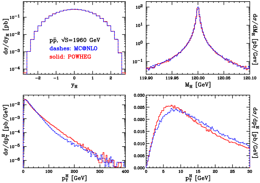
We have compared our results with MC@NLO, the only existing program where NLO Higgs boson production via gluon fusion is merged with a shower Monte Carlo program. Since MC@NLO uses only the HERWIG [5, 6] angular-ordered shower, we have also interfaced POWHEG with HERWIG, in order to minimize effects due to differences in the shower and hadronization algorithms.

MC@NLO generates the Higgs boson virtuality M2superscript𝑀2M^{2} according to the Breit-Wigner form

1πmHΓH(M2mH2)2+(mHΓH)2.1𝜋subscript𝑚𝐻subscriptΓ𝐻superscriptsuperscript𝑀2superscriptsubscript𝑚𝐻22superscriptsubscript𝑚𝐻subscriptΓ𝐻2\frac{1}{\pi}\frac{m_{H}\,\Gamma_{H}}{\left(M^{2}-m_{H}^{2}\right)^{2}+(m_{H}\,\Gamma_{H})^{2}}\,. (77)

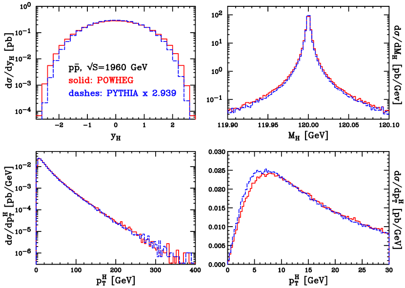
For the purpose of this comparison we have thus used the same form. We have considered two different sets of values for the Higgs boson mass and width: mH=120subscript𝑚𝐻120m_{H}=120 GeV with ΓH=3.605subscriptΓ𝐻3.605\Gamma_{H}=3.605 MeV and mH=400subscript𝑚𝐻400m_{H}=400 GeV with ΓH=28.89subscriptΓ𝐻28.89\Gamma_{H}=28.89 GeV.

Both in POWHEG and in MC@NLO there is the option to retain the full top-mass dependence in the Born cross section, i.e. to use a finite τQsubscript𝜏𝑄\tau_{Q} value in eq. (20). We have then the choice to generate our Born variables by fixing mt=171subscript𝑚𝑡171m_{t}=171 GeV in the B¯¯𝐵\bar{B} term in eq. (3.1) or by sending mtsubscript𝑚𝑡m_{t}\to\infty. Since we have computed the real-radiation term only in the mtsubscript𝑚𝑡m_{t}\to\infty limit, we have to use the same limit in the calculation of the Born term in the Sudakov form factor (70), in order to recover the correct Altarelli-Parisi behavior when the collinear limit is approached.

4.1.1 Tevatron results
Refer to caption
Figure 1: Comparison between POWHEG and MC@NLO for the rapidity, invariant mass and transverse-momentum distributions of a Higgs boson with mH=120subscript𝑚𝐻120m_{H}=120 GeV, at Tevatron pp¯𝑝¯𝑝p\bar{p} collider.
Refer to caption
Figure 2: Comparison between POWHEG and MC@NLO for the rapidity of the leading jet and the rapidity difference of the Higgs boson and the leading jet, defined according to the SISCONE algorithm, with different jet cuts.
Refer to caption
Figure 3: Comparison between POWHEG and MC@NLO for the transverse-momentum distributions of the leading jet, defined according to the SISCONE and the KT jet algorithms.

In fig. 1 we show a comparison between POWHEG and MC@NLO for the rapidity, invariant mass and transverse-momentum distributions of a Higgs boson with mass mH=120subscript𝑚𝐻120m_{H}=120 GeV, at the Tevatron pp¯𝑝¯𝑝p\bar{p} collider. The lowest order mtsubscript𝑚𝑡m_{t}-dependence is retained. A blowup of the transverse-momentum distribution near the low-pTsubscript𝑝Tp_{\mathchoice{\displaystyle}{\scriptstyle}{\scriptscriptstyle}{\scriptscriptstyle}\rm T} region is also shown. There is good agreement between the two programs, except for the transverse momentum distribution at high pTsubscript𝑝Tp_{\mathchoice{\displaystyle}{\scriptstyle}{\scriptscriptstyle}{\scriptscriptstyle}\rm T} (we will comment more on this issue in sec. 4.3).

In fig. 2 we compare the leading jet rapidity and the difference in the rapidity of the leading jet and the Higgs boson. The jet is defined using the SISCONE algorithm [25] as implemented in the FASTJET package [26], setting the jet radius R=0.7𝑅0.7R=0.7 and the overlapping fraction f=0.5𝑓0.5f=0.5. As in previous POWHEG implementations, we notice a dip in the MC@NLO jet rapidity distribution, which is enhanced in the difference. We have already extensively discussed this fact in sec. 4.3 of ref. [14].

In fig. 3, we compare the transverse-momentum distributions of the leading jet, reconstructed with the SISCONE and the kTsubscript𝑘𝑇k_{T} algorithms (included in FASTJET). A lower 101010 GeV cut on jet transverse momentum is imposed. The high-pTsubscript𝑝Tp_{\mathchoice{\displaystyle}{\scriptstyle}{\scriptscriptstyle}{\scriptscriptstyle}\rm T} discrepancy reflects the same behavior found for the Higgs boson transverse-momentum distribution (see sec. 4.3).

4.1.2 LHC results
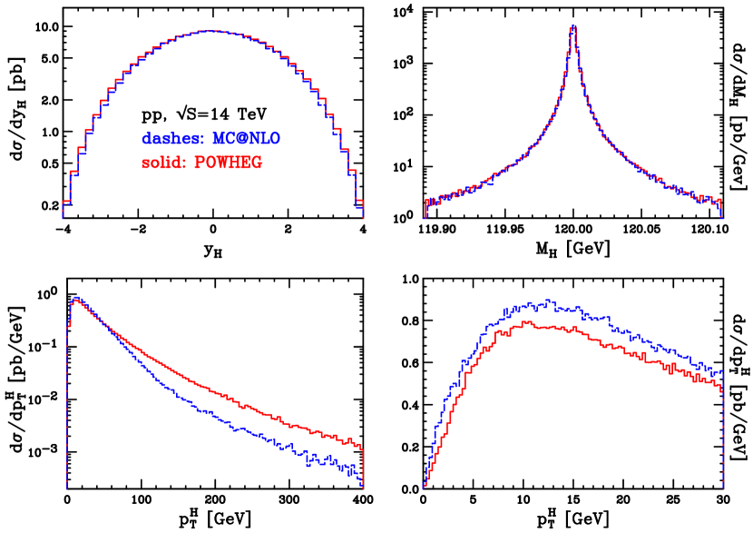
Refer to caption
Figure 4: Comparison between POWHEG and MC@NLO for the rapidity, invariant mass and transverse-momentum distributions of a Higgs boson with mH=120subscript𝑚𝐻120m_{H}=120 GeV, at the LHC pp𝑝𝑝pp collider.
Refer to caption
Figure 5: Comparison between POWHEG and MC@NLO for the rapidity of the leading jet and the rapidity difference of the Higgs boson and the leading jet, defined according to the SISCONE algorithm, with different jet cuts.
Refer to caption
Figure 6: Comparison between POWHEG and MC@NLO for the transverse-momentum distributions of the leading jet, defined according to the SISCONE and the KT algorithms.
Refer to caption
Figure 7: Comparison between POWHEG and MC@NLO for the rapidity, invariant mass and transverse-momentum distributions of a Higgs boson with mH=400subscript𝑚𝐻400m_{H}=400 GeV, at the LHC pp𝑝𝑝pp collider.
Refer to caption
Figure 8: Comparison between POWHEG and MC@NLO for the rapidity of the leading jet and the rapidity difference of the Higgs boson and the leading jet, defined according to the SISCONE algorithm, with different jet cuts.

From fig. 4 to 6 we carry out a similar analysis for the LHC pp𝑝𝑝pp collider. The difference in the hardness of the pTsubscript𝑝Tp_{\mathchoice{\displaystyle}{\scriptstyle}{\scriptscriptstyle}{\scriptscriptstyle}\rm T} distributions is more evident here than at the Tevatron. The other plots show instead a good agreement between the two codes, apart from the aforementioned dip in the leading-jet rapidity distributions.

We have also made some comparisons with a different value of the Higgs boson mass. We have chosen mH=400subscript𝑚𝐻400m_{H}=400 GeV, where the ratio between the Born cross sections evaluated with mt=171subscript𝑚𝑡171m_{t}=171 GeV and mtsubscript𝑚𝑡m_{t}\to\infty is close to its maximum value and roughly equals 3. The results are shown in fig. 7 and 8. We see that, in this case, the dip in the rapidity of the hardest jet in MC@NLO is extremely marked.

In the study of ref. [17], carried out in the framework of heavy-flavour production, the origin of the rapidity dip was tracked back to an even stronger dip in the pure HERWIG distribution, that the MC@NLO correction was not able to properly fill. The same pattern is also observed in the present context, as can be seen in fig. 9.
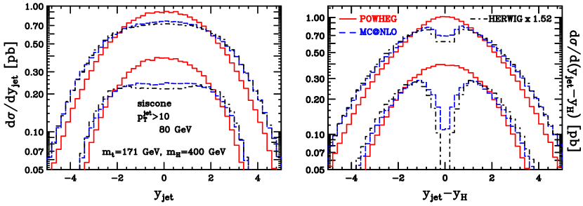
Refer to caption
Figure 9: Comparison of POWHEG, MC@NLO and HERWIG (without matrix-element corrections), for the rapidity of the leading jet and the rapidity difference of the Higgs boson and the leading jet, defined according to the SISCONE algorithm, with different jet cuts.

4.2 POWHEG - PYTHIA  comparison
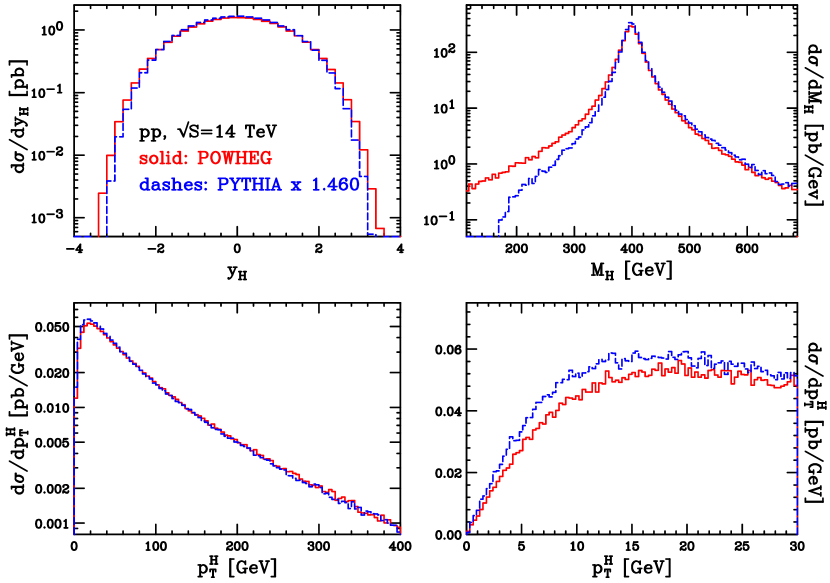
Refer to caption
Figure 10: Comparison between POWHEG and PYTHIA for the rapidity, invariant mass and transverse-momentum distributions of a Higgs boson with mH=120subscript𝑚𝐻120m_{H}=120 GeV, at Tevatron pp¯𝑝¯𝑝p\bar{p} collider. PYTHIA outputs normalized to the POWHEG cross section.
Refer to caption
Figure 11: Comparison between POWHEG and PYTHIA for the rapidity of the leading jet and the rapidity difference of the Higgs boson and the leading jet, defined according to the SISCONE algorithm, with different jet cuts. PYTHIA outputs are normalized to the POWHEG cross section.
Refer to caption
Figure 12: Comparison between POWHEG and PYTHIA for the transverse-momentum distributions of the leading jet, defined according to the SISCONE and the KT algorithms. PYTHIA outputs are normalized to the POWHEG cross section.
Refer to caption
Figure 13: Comparison between POWHEG and PYTHIA for the rapidity, invariant mass and transverse-momentum distributions of a Higgs boson with mH=120subscript𝑚𝐻120m_{H}=120 GeV, at the LHC. PYTHIA outputs are normalized to the POWHEG cross section.
Refer to caption
Figure 14: Comparison between POWHEG and PYTHIA for the rapidity of the leading jet and the rapidity difference of the Higgs boson and the leading jet, defined according to the SISCONE algorithm, with different jet cuts. PYTHIA outputs are normalized to the POWHEG cross section.
Refer to caption
Figure 15: Comparison between POWHEG and PYTHIA for the transverse-momentum distributions of the leading jet, defined according to the SISCONE and the KT algorithms. PYTHIA outputs are normalized to the POWHEG cross section.
Refer to caption
Figure 16: Comparison between POWHEG and PYTHIA for the rapidity, invariant mass and transverse-momentum distributions of a Higgs boson with mH=400subscript𝑚𝐻400m_{H}=400 GeV, at the LHC. PYTHIA outputs are normalized to the POWHEG cross section.

We now compare POWHEG and PYTHIA. The Higgs boson production implementation in PYTHIA includes matrix-element corrections, so that the pTsubscript𝑝Tp_{\mathchoice{\displaystyle}{\scriptstyle}{\scriptscriptstyle}{\scriptscriptstyle}\rm T} distribution of the Higgs boson is accurate at large pTsubscript𝑝Tp_{\mathchoice{\displaystyle}{\scriptstyle}{\scriptscriptstyle}{\scriptscriptstyle}\rm T}. In our comparisons, we always normalize the PYTHIA results to the full NLO cross section of POWHEG. We use the new pTsubscript𝑝Tp_{\mathchoice{\displaystyle}{\scriptstyle}{\scriptscriptstyle}{\scriptscriptstyle}\rm T}-ordered shower defined in the PYEVNW routine of PYTHIA, that should be more appropriate when interfacing to POWHEG.

The only difference with respect to the POWHEG-MC@NLO comparisons is in the generation of the Higgs boson virtuality, distributed now according to

1πM2ΓH/mH(M2mH2)2+(M2ΓH/mH)2,1𝜋superscript𝑀2subscriptΓ𝐻subscript𝑚𝐻superscriptsuperscript𝑀2superscriptsubscript𝑚𝐻22superscriptsuperscript𝑀2subscriptΓ𝐻subscript𝑚𝐻2\frac{1}{\pi}\frac{M^{2}\,\Gamma_{H}/m_{H}}{\left(M^{2}-m_{H}^{2}\right)^{2}+(M^{2}\,\Gamma_{H}/m_{H})^{2}}\,, (78)

which is very similar to the form used in PYTHIA, except for the fact that PYTHIA includes threshold effects in the calculation of the Higgs boson width. In fact, PYTHIA uses a running ΓH(M2)subscriptΓ𝐻superscript𝑀2\Gamma_{H}(M^{2}), that increases when a decay channel opens up. The effects of using a fixed or a running ΓHsubscriptΓ𝐻\Gamma_{H} are more evident for a heavy Higgs boson, as will be shown in the following.

In figs. 10 through 12 we compare results for the Tevatron pp¯𝑝¯𝑝p\bar{p} collider, while in figs. 13 through 15 we present results for the LHC. In all the plots we have set mH=120subscript𝑚𝐻120m_{H}=120 GeV. Results are in an impressive good agreement, both for inclusive quantities and for more exclusive ones. The only visible difference is in the transverse Higgs boson momentum distribution at low pTsubscript𝑝Tp_{\mathchoice{\displaystyle}{\scriptstyle}{\scriptscriptstyle}{\scriptscriptstyle}\rm T} at the LHC. This could be due to the different choice of the renormalization and factorization scale in the generation of radiation, our choice being constrained by the requirement of next-to-leading logarithmic accuracy in the Sudakov form factor.

In fig. 16 we present a comparison with mH=400subscript𝑚𝐻400m_{H}=400 GeV. Mass thresholds effects in ΓHsubscriptΓ𝐻\Gamma_{H} are evident in the invariant-mass distribution generated by PYTHIA. Below 2mt2subscript𝑚𝑡2\,m_{t} the total width is smaller than the fixed one we are using, and PYTHIA results are accordingly lower than ours. All other plots show instead good agreement with POWHEG.

The good agreement between POWHEG and PYTHIA was to some extent expected. As already observed in refs. [9, 14], the matrix-element correction method used in PYTHIA [27, 28] bears considerable similarities to POWHEG.

4.3 The 𝒑𝐓subscript𝒑𝐓\boldsymbol{p_{\mathchoice{\displaystyle}{\scriptstyle}{\scriptscriptstyle}{\scriptscriptstyle}\rm T}} distribution in POWHEG

Refer to caption
Figure 17: Comparison between POWHEG, MC@NLO and the NLO calculation, for mH=120subscript𝑚𝐻120m_{H}=120 GeV at the LHC. All calculations are performed in the mtsubscript𝑚𝑡m_{t}\to\infty approximation. Shower and hadronization are included in the MC results. The POWHEG result is also presented without shower and hadronization, and with a fixed-scale choice.
Refer to caption
Figure 18: Comparison between POWHEG and fixed NLO and NNLO distributions for the transverse-momentum of the Higgs boson. Plots are done for mH=120subscript𝑚𝐻120m_{H}=120 GeV at the LHC.

In this section we address the discrepancy in the pTsubscript𝑝Tp_{\mathchoice{\displaystyle}{\scriptstyle}{\scriptscriptstyle}{\scriptscriptstyle}\rm T} distributions in POWHEG and in MC@NLO. First of all, we show in fig. 17 a comparison between the pTsubscript𝑝Tp_{\mathchoice{\displaystyle}{\scriptstyle}{\scriptscriptstyle}{\scriptscriptstyle}\rm T} spectrum of POWHEG, MC@NLO and the NLO calculation. For sake of comparison, we have used in POWHEG and in the NLO calculation the same scale choice adopted in MC@NLO. We point out, however, that using a scale that depends upon the transverse momentum of radiation in POWHEG can only affect the B¯¯𝐵\bar{B} function. More specifically, one ends up using a transverse momentum dependent scale only in calculation of the real contributions in B¯¯𝐵\bar{B}, since the transverse momentum is zero for the Born, virtual and collinear remnant terms. Thus, this scale does not depend upon the transverse momentum of the real radiation, that is generated afterwards using the POWHEG Sudakov form factor. The choice of scale for radiation affects instead a single power of the coupling constant, since the Sudakov exponent is proportional to αSsubscript𝛼S\alpha_{\mathchoice{\displaystyle}{\scriptstyle}{\scriptscriptstyle}{\scriptscriptstyle}\rm S}. At low transverse momentum, this scale cannot be changed without spoiling the NLL accuracy of the Sudakov form factor. It can be changed, however, at large transverse momentum to explore further uncertainties. However, we have preferred not to implement this possibility. One should recall, in fact, that this scale only affects a single power of αSsubscript𝛼S\alpha_{\mathchoice{\displaystyle}{\scriptstyle}{\scriptscriptstyle}{\scriptscriptstyle}\rm S}, and it thus has a much smaller effect than a scale change in the NLO cross section.

We see from fig. 17 that MC@NLO agrees better than POWHEG with the NLO calculation at large pTsubscript𝑝Tp_{\mathchoice{\displaystyle}{\scriptstyle}{\scriptscriptstyle}{\scriptscriptstyle}\rm T}. Since the difference between MC@NLO and POWHEG should be of next-to-next-to-leading order (NNLO), the difference between POWHEG and the NLO result should also be of NNLO. In fact we can easily trace the origin of this difference. From eq. (76), we infer that, at large pTsubscript𝑝Tp_{\mathchoice{\displaystyle}{\scriptstyle}{\scriptscriptstyle}{\scriptscriptstyle}\rm T}, the POWHEG differential cross section can be written as

dσ=[B¯(𝚽¯1)R(𝚽2)B(𝚽¯1)+qRqq¯(𝚽2)]d𝚽¯1dΦrad,𝑑𝜎delimited-[]¯𝐵subscript¯𝚽1𝑅subscript𝚽2𝐵subscript¯𝚽1subscript𝑞subscript𝑅𝑞¯𝑞subscript𝚽2𝑑subscript¯𝚽1𝑑subscriptΦradd\sigma=\left[\bar{B}(\bar{\bf\Phi}_{1})\,\frac{R\left({\bf\Phi}_{2}\right)}{B\!\left(\bar{\bf\Phi}_{1}\right)}+\sum_{q}R_{q\bar{q}}\left({\bf\Phi}_{2}\right)\right]\,d\bar{\bf\Phi}_{1}\,d\Phi_{\rm rad}\,, (79)

since the Sudakov form factor approaches 1 in this region. Neglecting the subdominant qq¯𝑞¯𝑞q\bar{q} real contribution, this differs from the pure NLO result because of the presence of the factor

B¯(𝚽¯1)B(𝚽¯1)=1+𝒪(αS).¯𝐵subscript¯𝚽1𝐵subscript¯𝚽11𝒪subscript𝛼S\frac{\bar{B}(\bar{\bf\Phi}_{1})}{B\!\left(\bar{\bf\Phi}_{1}\right)}=1+{\cal O}(\alpha_{\mathchoice{\displaystyle}{\scriptstyle}{\scriptscriptstyle}{\scriptscriptstyle}\rm S})\;. (80)

It is known that radiative corrections in Higgs boson production are large, so that the 𝒪(αS)𝒪subscript𝛼S{\cal O}(\alpha_{\mathchoice{\displaystyle}{\scriptstyle}{\scriptscriptstyle}{\scriptscriptstyle}\rm S}) term is in fact of order 1, and thus we find an enhancement that approaches a factor of two.333We recall that normally the numerator and denominator in this factor are evaluated at different scales, since in B¯¯𝐵\bar{B} one uses a scale of the order of the Higgs boson transverse mass, while in the B𝐵B term, one uses the transverse momentum. However, at large pTsubscript𝑝Tp_{\mathchoice{\displaystyle}{\scriptstyle}{\scriptscriptstyle}{\scriptscriptstyle}\rm T}, the two scales become of the same order. We have performed a clear cut test of this interpretation of the discrepancy. We have replaced the B¯¯𝐵\bar{B} function with the Born term B𝐵B in the POWHEG program. The result of this calculation is shown in comparison with the NLO curve in fig. 18. Since, as shown in fig. 17, the shower and hadronization are irrelevant for this distribution, we do not include them in the figure. In fig. 18 we have chosen to use pTsubscript𝑝Tp_{\mathchoice{\displaystyle}{\scriptstyle}{\scriptscriptstyle}{\scriptscriptstyle}\rm T} independent renormalization and factorization scales, in order to perform a consistent comparison. Notice that, with this choice of scales, the NLO distribution is harder than the one shown in fig. 17. This is easily explained by the fact that the NLO process is proportional to αS3(μR)superscriptsubscript𝛼S3subscript𝜇R\alpha_{\mathchoice{\displaystyle}{\scriptstyle}{\scriptscriptstyle}{\scriptscriptstyle}\rm S}^{3}(\mu_{\mathchoice{\displaystyle}{\scriptstyle}{\scriptscriptstyle}{\scriptscriptstyle}\rm R}), and thus a pTsubscript𝑝Tp_{\mathchoice{\displaystyle}{\scriptstyle}{\scriptscriptstyle}{\scriptscriptstyle}\rm T} dependent renormalization scale can alter significantly the pTsubscript𝑝Tp_{\mathchoice{\displaystyle}{\scriptstyle}{\scriptscriptstyle}{\scriptscriptstyle}\rm T} distribution.

At this point, we can ask whether the higher order terms included in POWHEG with the mechanism illustrated above do in fact give a reasonable estimate of true NNLO effects. We thus include in fig. 18 the NNLO result, obtained from the HNNLO program of ref. [16]. The result shows a rather good agreement between the NNLO result and POWHEG. Thus, our seemingly large corrections to the Higgs boson pTsubscript𝑝Tp_{\mathchoice{\displaystyle}{\scriptstyle}{\scriptscriptstyle}{\scriptscriptstyle}\rm T} distributions are in fact very similar in size to the full NNLO result. Observe that in fig. 18 we have used a fixed scale choice for all the results. We were forced to do this, since the HNNLO program does not allow for other choices. However, because of the good agreement of the two POWHEG results in fig. 17, and because of the smaller scale dependence of the NNLO result, this should not make a severe difference.

Because of a fortuitous circumstance, we did not need to worry about correcting for the large difference between the POWHEG and the NLO result at large radiation transverse momentum, since the known NNLO result seems to support the POWHEG one. We remark, however, that, had this not been the case, it is very easy to modify the POWHEG algorithm so to obtain a pTsubscript𝑝Tp_{\mathchoice{\displaystyle}{\scriptstyle}{\scriptscriptstyle}{\scriptscriptstyle}\rm T} spectrum that agrees with the NLO calculation at large pTsubscript𝑝Tp_{\mathchoice{\displaystyle}{\scriptstyle}{\scriptscriptstyle}{\scriptscriptstyle}\rm T}. This can be done as follows. Instead of using the full real cross section for the computation of the B¯¯𝐵\bar{B} function and of the Sudakov form factor, we can instead use a reduced real contribution

Rred=R×F,superscript𝑅red𝑅𝐹R^{\rm red}=R\times F\,, (81)

where F𝐹F is a function of the real phase space, with F<1𝐹1F<1 everywhere, such that F𝐹F approaches 1 for small transverse momenta, and approaches zero for large transverse momenta. We perform the POWHEG generation using Rredsuperscript𝑅redR^{\rm red} instead of R𝑅R, and treat the remaining R×(1F)𝑅1𝐹R\times(1-F) contribution to the cross section with the same method that we used for the Rqq¯subscript𝑅𝑞¯𝑞R_{q\bar{q}} contribution. This can be done, since R×(1F)𝑅1𝐹R\times(1-F) is dumped by the 1F1𝐹1-F factor in the singular region. It will then follow that, for large transverse momentum, the result would agree with the NLO calculation, since it would be dominated by the R×(1F)𝑅1𝐹R\times(1-F) contribution. It turned out that, in all previous implementations, it was not necessary to use such procedure. As remarked before, thanks to the known properties of the NNLO result, this was not necessary even in this case. We have however performed such study, just in order to illustrate the flexibility of the POWHEG method. We have chosen for F𝐹F the following form

F=h2pT2+h2.𝐹superscript2superscriptsubscript𝑝T2superscript2F=\frac{h^{2}}{p_{\mathchoice{\displaystyle}{\scriptstyle}{\scriptscriptstyle}{\scriptscriptstyle}\rm T}^{2}+h^{2}}\,. (82)

The resulting transverse-momentum distribution at the LHC, for a Higgs boson mass of 400 GeV, is shown in fig. 19 for hh\to\infty (standard POWHEG), h=120120h=120 GeV and h=400400h=400 GeV.

Refer to caption
Figure 19: Comparison of the predictions of MC@NLO, standard POWHEG (hh\to\infty) and POWHEG with two different values of the parameter hh (h=120120h=120 GeV and h=mH=400subscript𝑚𝐻400h=m_{H}=400 GeV) in the function F𝐹F of eq. (82), for the transverse-momentum distributions of a Higgs boson, at the LHC pp𝑝𝑝pp collider.

One can see that it is not difficult to get distributions that undershoot the MC@NLO one in the intermediate range of pTsubscript𝑝Tp_{\mathchoice{\displaystyle}{\scriptstyle}{\scriptscriptstyle}{\scriptscriptstyle}\rm T}. We also observe that, with this procedure, no undesired features of other distributions appear. In particular, the distribution in the rapidity of the hardest jet, and in the rapidity difference between the hardest jet and the Higgs boson remain qualitatively the same, as shown in fig. 20.
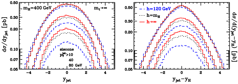
Refer to caption
Figure 20: Comparison of the predictions of the standard POWHEG (hh\to\infty), and POWHEG with two different values of the parameter hh (h=120120h=120 GeV and h=mH=400subscript𝑚𝐻400h=m_{H}=400 GeV) in the function F𝐹F of eq. (82), for the rapidity of the leading jet and the rapidity difference of the Higgs boson and the leading jet, defined according to the SISCONE algorithm, with different jet cuts, at the LHC.

4.4 Next-to-leading logarithmic resummation
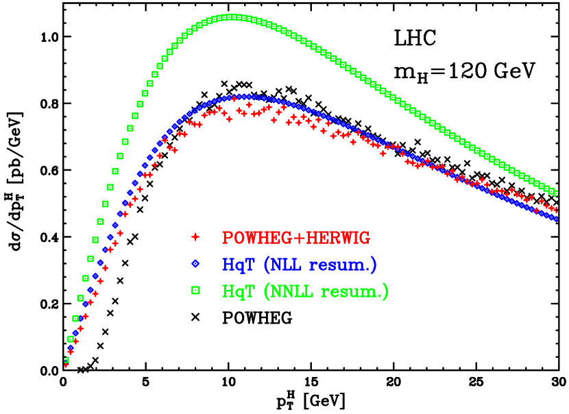
Refer to caption
Figure 21: Comparison between POWHEG and HqT for the transverse-momentum distributions of a Higgs boson, at the LHC. The POWHEG result without shower and hadronization is also shown.

As explained in section (4.4) of ref. [9], one can reach next-to-leading logarithmic (NLL) accuracy of soft gluon resummation if the number of coloured partons involved in the hard scattering is less or equal to three. This can be obtained by replacing the strong coupling constant in the Sudakov exponent with [29]

αSA(αS(kT2)),A(αS)=αS{1+αS2π[(6718π26)CA59nf]},formulae-sequencesubscript𝛼S𝐴subscript𝛼Ssuperscriptsubscript𝑘T2𝐴subscript𝛼Ssubscript𝛼S1subscript𝛼S2𝜋delimited-[]6718superscript𝜋26subscript𝐶A59subscript𝑛f\alpha_{\mathchoice{\displaystyle}{\scriptstyle}{\scriptscriptstyle}{\scriptscriptstyle}\rm S}\rightarrow A\left(\alpha_{\mathchoice{\displaystyle}{\scriptstyle}{\scriptscriptstyle}{\scriptscriptstyle}\rm S}\left(k_{\mathchoice{\displaystyle}{\scriptstyle}{\scriptscriptstyle}{\scriptscriptstyle}\rm T}^{2}\right)\right),\qquad A(\alpha_{\mathchoice{\displaystyle}{\scriptstyle}{\scriptscriptstyle}{\scriptscriptstyle}\rm S})=\alpha_{\mathchoice{\displaystyle}{\scriptstyle}{\scriptscriptstyle}{\scriptscriptstyle}\rm S}\left\{1+\frac{\alpha_{\mathchoice{\displaystyle}{\scriptstyle}{\scriptscriptstyle}{\scriptscriptstyle}\rm S}}{2\pi}\left[\left(\frac{67}{18}-\frac{\pi^{2}}{6}\right)C_{\mathchoice{\displaystyle}{\scriptstyle}{\scriptscriptstyle}{\scriptscriptstyle}\rm A}-\frac{5}{9}n_{\rm f}\right]\right\}, (83)

where the MS¯¯MS\overline{{\rm MS}}, 1-loop expression of αSsubscript𝛼S\alpha_{\mathchoice{\displaystyle}{\scriptstyle}{\scriptscriptstyle}{\scriptscriptstyle}\rm S} should be used. The previous replacement may also be implemented by a simple redefinition of the strong scale ΛΛ\Lambda, which, for five active flavours (nf=5subscript𝑛f5n_{\rm f}=5), becomes ΛMC1.569ΛMS¯(5)subscriptΛMC1.569superscriptsubscriptΛ¯MS5\Lambda_{\scriptscriptstyle\rm{MC}}\equiv 1.569\,\Lambda_{\scriptscriptstyle\overline{\rm MS}}^{(5)}. We have exploited this possibility in our code, so that our result should agree with the NLL resummed one. A comparison has been thus carried out with the HqT [30] program, that performs such a resummation. We have adopted fixed renormalization and factorization scales. Results are shown in fig. 21, together with next-to-next-to-leading logarithmic (NNLL) resummation, always from HqT, just for reference purposes. We see a fair agreement between the POWHEG result and the NLL analytic one, as expected. The different behaviour of the POWHEG result without shower and hadronization at very low pTsubscript𝑝Tp_{\mathchoice{\displaystyle}{\scriptstyle}{\scriptscriptstyle}{\scriptscriptstyle}\rm T} may be ascribed to the particular implementation of the minimum transverse momentum that we use, that is, to a large extent, arbitrary.

We observe that, in all cases, we do not expect full agreement between the POWHEG result without shower, and the NLL calculation. In fact, the POWHEG curve without shower represents the Sudakov form factor for the pTsubscript𝑝Tp_{\mathchoice{\displaystyle}{\scriptstyle}{\scriptscriptstyle}{\scriptscriptstyle}\rm T} of the hardest emission, while, in the NLL calculation, the total pTsubscript𝑝Tp_{\mathchoice{\displaystyle}{\scriptstyle}{\scriptscriptstyle}{\scriptscriptstyle}\rm T} distribution (i.e. the sum of the transverse momenta of all emissions) is considered. Thus, it is only after the inclusion of the full shower effects that the two distributions have a meaningful comparison.

5 Conclusions

In this paper we have reported on a complete implementation of Higgs boson production via gluon fusion at next-to-leading order in QCD, in the POWHEG framework. The calculation was performed within the Frixione-Kunszt-Signer [20, 21] subtraction approach. We have also shown how to deal with non-singular real contributions, that do not present a valid underlying Born matrix element.

The results of our work have been compared extensively with MC@NLO and PYTHIA shower Monte Carlo programs. The PYTHIA results, normalized to the total NLO cross section, are in good agreement with POWHEG, except for differences in the low transverse-momentum distributions of the Higgs boson at the LHC. The MC@NLO results are in fair agreement with POWHEG, except for the pTsubscript𝑝Tp_{\mathchoice{\displaystyle}{\scriptstyle}{\scriptscriptstyle}{\scriptscriptstyle}\rm T} distribution of the Higgs boson, and consequently of the hardest jet, in the high-pTsubscript𝑝Tp_{\mathchoice{\displaystyle}{\scriptstyle}{\scriptscriptstyle}{\scriptscriptstyle}\rm T} region. In this region the POWHEG distributions are generally harder. We have shown that this is due to NNLO effects in the POWHEG formula for the differential cross section. We checked that these effects actually bring our result closer to the NNLO one [16]. The low-pTsubscript𝑝Tp_{\mathchoice{\displaystyle}{\scriptstyle}{\scriptscriptstyle}{\scriptscriptstyle}\rm T} region was instead tested against the analytic resummed results [30]. We find again good agreement up to NLL accuracy.

Furthermore, we have also examined the distributions in the difference of the hardest jet and the Higgs boson rapidity. The dip found in previous implementations [10, 11, 14] is still present. We remark that this seems to be a general feature of MC@NLO, since other calculations do not find effects of this kind [17, 18, 19].

The computer code for the POWHEG implementations presented in this paper is available, together with the manual, at the site

http://moby.mib.infn.it/~nason/POWHEG

References

  • [1] S. Dawson, Radiative corrections to Higgs boson production, Nucl. Phys. B359 (1991) 283–300.
  • [2] A. Djouadi, M. Spira, and P. M. Zerwas, Production of Higgs bosons in proton colliders: QCD corrections, Phys. Lett. B264 (1991) 440–446.
  • [3] M. Spira, A. Djouadi, D. Graudenz, and P. M. Zerwas, Higgs boson production at the LHC, Nucl. Phys. B453 (1995) 17–82, [hep-ph/9504378].
  • [4] S. Frixione and B. R. Webber, Matching NLO QCD computations and parton shower simulations, JHEP 06 (2002) 029, [hep-ph/0204244].
  • [5] G. Corcella et al., HERWIG 6: An event generator for hadron emission reactions with interfering gluons (including supersymmetric processes), JHEP 01 (2001) 010, [hep-ph/0011363].
  • [6] G. Corcella et al., Herwig 6.5 release note, hep-ph/0210213.
  • [7] T. Sjostrand, S. Mrenna, and P. Skands, Pythia 6.4 physics and manual, JHEP 05 (2006) 026, [hep-ph/0603175].
  • [8] P. Nason, A new method for combining NLO QCD with shower Monte Carlo algorithms, JHEP 11 (2004) 040, [hep-ph/0409146].
  • [9] S. Frixione, P. Nason, and C. Oleari, Matching NLO QCD computations with Parton Shower simulations: the POWHEG method, JHEP 11 (2007) 070, [arXiv:0709.2092 [hep-ph]].
  • [10] P. Nason and G. Ridolfi, A positive-weight next-to-leading-order Monte Carlo for Z𝑍Z pair hadroproduction, JHEP 08 (2006) 077, [hep-ph/0606275].
  • [11] S. Frixione, P. Nason, and G. Ridolfi, A Positive-Weight Next-to-Leading-Order Monte Carlo for Heavy Flavour Hadroproduction, JHEP 09 (2007) 126, [arXiv:0707.3088 [hep-ph]].
  • [12] O. Latunde-Dada, S. Gieseke, and B. Webber, A positive-weight next-to-leading-order Monte Carlo for e+esuperscript𝑒superscript𝑒e^{+}e^{-} annihilation to hadrons, JHEP 02 (2007) 051, [hep-ph/0612281].
  • [13] O. Latunde-Dada, Applying the POWHEG method to top pair production and decays at the ILC, 0806.4560.
  • [14] S. Alioli, P. Nason, C. Oleari, and E. Re, NLO vector-boson production matched with shower in POWHEG, JHEP 07 (2008) 060, [0805.4802].
  • [15] K. Hamilton, P. Richardson, and J. Tully, A Positive-Weight Next-to-Leading Order Monte Carlo Simulation of Drell-Yan Vector Boson Production, JHEP 10 (2008) 015, [0806.0290].
  • [16] S. Catani and M. Grazzini, An NNLO subtraction formalism in hadron collisions and its application to Higgs boson production at the LHC, Phys. Rev. Lett. 98 (2007) 222002, [hep-ph/0703012].
  • [17] M. L. Mangano, M. Moretti, F. Piccinini, and M. Treccani, Matching matrix elements and shower evolution for top-quark production in hadronic collisions, JHEP 01 (2007) 013, [hep-ph/0611129].
  • [18] J. Alwall et al., Comparative study of various algorithms for the merging of parton showers and matrix elements in hadronic collisions, Eur. Phys. J. C53 (2008) 473–500, [arXiv:0706.2569 [hep-ph]].
  • [19] S. Dittmaier, P. Uwer, and S. Weinzierl, Hadronic top-quark pair production in association with a hard jet at next-to-leading order QCD: Phenomenological studies for the Tevatron and the LHC, arXiv:0810.0452 [hep-ph].
  • [20] S. Frixione, Z. Kunszt, and A. Signer, Three-jet cross sections to next-to-leading order, Nucl. Phys. B467 (1996) 399–442, [hep-ph/9512328].
  • [21] S. Frixione, A general approach to jet cross sections in QCD, Nucl. Phys. B507 (1997) 295–314, [hep-ph/9706545].
  • [22] P. Nason, MINT: a Computer Program for Adaptive Monte Carlo Integration and Generation of Unweighted Distributions, arXiv:0709.2085 [hep-ph].
  • [23] P. Nason and G. Ridolfi, A positive-weight next-to-leading-order Monte Carlo for Z𝑍Z pair hadroproduction, JHEP 08 (2006) 077, [hep-ph/0606275].
  • [24] J. Pumplin et al., New generation of parton distributions with uncertainties from global QCD analysis, JHEP 07 (2002) 012, [hep-ph/0201195].
  • [25] G. P. Salam and G. Soyez, A practical Seedless Infrared-Safe Cone jet algorithm, JHEP 05 (2007) 086, [arXiv:0704.0292 [hep-ph]].
  • [26] M. Cacciari and G. P. Salam, Dispelling the N3superscript𝑁3N^{3} myth for the kTsubscript𝑘𝑇k_{T} jet-finder, Phys. Lett. B641 (2006) 57–61, [hep-ph/0512210].
  • [27] M. Bengtsson and T. Sjostrand, Coherent Parton Showers Versus Matrix Elements: Implications of PETRA - PEP Data, Phys. Lett. B185 (1987) 435.
  • [28] T. Sjostrand, Monte Carlo generators, hep-ph/0611247.
  • [29] S. Catani, B. R. Webber, and G. Marchesini, QCD coherent branching and semiinclusive processes at large x𝑥x, Nucl. Phys. B349 (1991) 635–654.
  • [30] G. Bozzi, S. Catani, D. de Florian, and M. Grazzini, Transverse-momentum resummation and the spectrum of the Higgs boson at the LHC, Nucl. Phys. B737 (2006) 73–120, [hep-ph/0508068].