Lab/UFR-HEP-0807-rev/GNPHE-0807-rev
Topological String on Toric CY3s in Large Complex Structure Limit

Abstract

We develop a non planar topological vertex formalism and we use it to study the A-model partition function $\mathcal{Z}_{top}$ of topological string on the class of toric Calabi-Yau threefolds (CY3) in large complex structure limit. To that purpose, we first consider the $T^{2}\times R$ special Lagrangian fibration of generic CY3-folds and we give the realization of the class of large $\mu$ toric CY3-folds in terms of supersymmetric gauged linear sigma model with non zero gauge invariant superpotentials $\mathcal{W}\left(\Phi\right)$. Then, we focus on a one complex parameter supersymmetric $U\left(1\right)$ gauged model involving six chiral superfields $\left\{\Phi_{i}\right\}$ with $\mathcal{W}=\mu\left(\prod\nolimits_{i=0}^{5}\Phi_{i}\right)$ and we use it to compute the function $\mathcal{Z}_{top}$ for the case of the local elliptic curve in the limit $\mu\rightarrow\infty$.
Key words: CY3-folds with large complex structures, topological string theory on CY3s, topological 3-vertex formalism and beyond.
E-mails:   drissilb@gmail.com,   jehjouh@gmail.com,   h-saidi@fsr.ac.ma

1 Introduction

The discovery of topological tri-vertex formalism by Aganagic et al [1] and the developments that followed [2]-[17] have given a big impulse to the study of topological string on local Calabi-Yau threefolds $X_{3}$. Amongst the multiple results obtained in this direction, we mention too particularly: (i) the explicit computation of the A model topological string amplitudes for the set of toric Calabi-Yau threefolds (CY3s) [1, 8]. (ii) the works of Bryan and Pandharipande who determined completely the local invariants of nonsingular g-genus curves [31, 32]; and (iii) the derivation of the generating function of Gromov–Witten invariants of toric Calabi–Yau threefolds, which can be also expressed in terms of the topological vertex [33]. However, in most of these studies, a special interest has been devoted to topological strings on those toric CY3s which have a realization in terms of $2D$ $\mathcal{N}=2$ supersymmetric gauged linear sigma model without chiral matter superpotential; that is $\mathcal{W}\left(\Phi\right)=0$.
In this paper, we investigate the general situation where non zero chiral superpotentials $\mathcal{W}\left(\Phi\right)\neq 0$ are implemented and we study topological strings on that special class of toric Calabi-Yau threefolds $H_{3}$ describing backgrounds with $\mathcal{W}\left(\Phi\right)\neq 0$.
For this case, $\mathcal{W}\left(\Phi\right)\neq 0$, we will show amongst others that the topological vertex formalism involves a non planar (np) topological vertex C^(np) rather than the standard planar one of ref [1]. Moreover, considering toric CY3s $H_{3}$ embedded in complex Kahler 4-folds $\mathcal{X}_{4}$; we show equally that their topological vertex C^(np) shares basic features of the topological 4- vertex associated with the ambient space $\mathcal{X}_{4}$. The interpretation of C^(np) in terms of 3d- partitions was exhibited in [18]; but here we make a step further towards a formalism based on 2d-partitions by mainly using the decomposition property of 3d- partitions (known as well as plane partitions) in terms of Young diagrams [19, 20, 34].
Before going ahead, it is interesting to note that to deal with C^(np) with rigor, sophisticated mathematical tools are needed. Below, we will use rather a physical approach to shed more light on C^(np) by taking advantage of the link between Calabi-Yau manifolds and supersymmetric gauged linear sigma models. In this optic, we first give useful tools on toric geometry [21, 22, 23] by focusing on the T${}^{2}\times R$ special Lagrangian fibration of Calabi-Yau threefolds [24, 25, 26] associated to supersymmetric linear sigma models with non zero gauge invariant superpotentials $\mathcal{W}\left(\Phi\right)$. Then, we study the explicit expressions of the various hamiltonians of the $T^{2}\times R$ fibration of toric CY3s and we determine explicitly the values of the shrinking cycles of the non planar vertices solving the Calabi-Yau condition. This CY condition is physically interpreted in terms of the conservation of total momenta at each vertex of the toric web diagram in the same spirit as in the case of Feynman graph vertices of quantum field theory (QFT).
As an illustration of the construction, we compute the A model topological string partition function of the local elliptic curve in the large complex structure limit by using the cutting and gluing method gotten by mimicking the Aganagic et al approach.

The organization of this paper is as follows: In section 2, we briefly describe the supersymmetric field theoretical set up of Calabi-Yau threefolds with large complex structures. In section 3, we introduce helpful tools for later use. We study the toric representations of local normal bundle $NP^{n-1}$ for lower values of $n\leq 4$, by using supersymmetric gauged linear sigma model. We also give useful results on these toric CY3s, make comments on $T^{n-1}\times R$ special Lagrangian fibration and determine the corresponding hamiltonians. In section 4, we study the simplest example involving one gauge superfield $V$ and six chiral superfields $\left\{\Phi_{0},\Phi_{1},\Phi_{2},\Phi_{3},\Phi_{4},\Phi_{5}\right\}$ with chiral superpotential $\mathcal{W}\left(\Phi\right)=\mathrm{\mu}\prod\nolimits_{i=0}^{5}\Phi_{i},$ $\mu\neq 0$. This gauge invariant superfield model describes the local 2-torus in the large complex structure limit. In section 5, we study the topological vertex formalism for topological string on the local elliptic curve by using the non planar vertex . In section 6, we give a conclusion and perspectives and in section 7, we give an appendix on local Gromov–Witten invariants of curves in a Calabi–Yau threefold [8, 31] and their relationship with the non planar topological vertex presented in this paper.

2 CY3s in large complex structure limit

To deal with the field theoretical set up of the complex deformations of CY3s captured by gauge invariant chiral superpotential monomials, we start by recalling the $2D$ $\mathcal{N}=2$ supersymmetric (or equivalently $4D$ $\mathcal{N}=1$) gauged linear sigma model with Lagrangian density [27],

$$L_{0}\left(x\right)=\int d^{2}\theta d^{2}\overline{\theta}\mathcal{L}\left(\Phi_{i},V_{a},\overline{\Phi}_{i};t^{a}\right)$$ ,

(2.1)

describing the Kahler deformations of CY3s. In this relation, the Lagrangian super- density $\mathcal{L}\left(\Phi_{i},V_{a},\overline{\Phi}_{i};t^{a}\right)$ is invariant under the following $U^{r}\left(1\right)$ abelian gauge symmetry,

$$\Phi_{i}^{\prime}=\left(e^{\mathrm{i}\left(\sum_{a=1}^{r}\mathrm{q}_{i}^{a}\Lambda_{a}\right)}\right)\Phi_{i},$$ ,

,

(2.2)

with the $\mathrm{q}_{i}^{a}$ integers being the gauge charges of the matter superfields and $\Lambda_{a}$ standing for chiral superfield gauge parameters. The real superfields

$$V^{a}\sim\left(A_{\mu}^{a},\text{ }\lambda_{\text{{\tiny Majorana}}}^{a},\text{ }D^{a}\right),$$ (2.3)

appearing in eq(2.1) are $U^{r}\left(1\right)$ abelian gauge superfields; the $t^{a}$s are Kahler parameters and the hermitian super- density $\mathcal{L}\left(\Phi_{i},V_{a},\overline{\Phi}_{i};t^{a}\right)$ describes the gauge invariant interacting dynamics of the $2D$ $\mathcal{N}=2$ chiral superfields $\Phi_{i}$ and $\overline{\Phi}_{i}$.

D-terms and CY3s
In this field theoretical formulation, the defining equation of local Calabi-Yau threefolds $X_{3}$ is given by the usual equations of motion of the auxiliary D-terms

$$X_{3}:\qquad\frac{\delta L_{0}}{\delta D_{a}}=\sum_{i=1}^{3+r}q_{i}^{a}\left|\phi_{i}\right|^{2}-t^{a}=0,\qquad a=1,...,r$$ ,

(2.4)

where $\phi_{i}=\Phi_{i}$$|$_θ=0 are complex scalar fields, often denoted as $z_{i}$, and where the real numbers $t^{a}$ are the Fayet-Iliopoulos (FI) real coupling constants. The real numbers $t^{a}$’s are interpreted geometrically as Kahler parameters capturing Kahler deformations of the toric CY3 (2.4). The Calabi-Yau condition, requiring the vanishing of the first Chern class $\mathcal{C}_{1}\left(X_{3}\right)=0$, translates in the superfield approach into the following condition on the $U^{r}\left(1\right)$ charges $q_{i}^{a}$ of the matter superfields;

$$\sum_{i=1}^{n}q_{i}^{a}=0,\qquad a=1,...,n-3,$$ (2.5)

encoding the conformal behavior of the field theoretic model in the infrared [28, 29, 30].

Eqs(2.1-2.5) are very well known in literature and they are not our main purpose here; they are just tools towards the study of topological strings on a special class of toric Calabi-Yau threefolds $H_{3}$ going beyond the set of $X_{3}$’s described by eq(2.4). Below, we shall give details on the construction of the $H_{3}$s; but before notice that our interest into this class of CY3s have been first motivated by looking for the extension of the Aganagic et al topological 3- vertex formalism to the general case where the interacting gauge invariant dynamics of the scalar fields $\phi_{i}$ contain, in addition to the usual gauge-matter couplings namely,

$$\int d^{4}\theta\sum_{a}\left(\sum_{i}q_{i}^{a}V_{a}\left|\Phi^{i}\right|^{2}-t^{a}V_{a}\right),$$ (2.6)

matter self- interactions captured by a non zero superpotential $\mathcal{W}\left(\Phi\right)$ [27]-[29].

F- terms and the class of H₃ CY3s
In the case where there are matter self- interactions, $\mathcal{W}\left(\Phi\right)\neq 0$, the above Lagrangian density $L_{0}$ extends as,

$$L=L_{0}+\int d^{2}\theta\mathcal{W}\left(\Phi_{1},..,\Phi_{n};\mu_{i}\right)+\int d^{2}\overline{\theta}\overline{\mathcal{W}}\left(\overline{\Phi}_{1},..,\overline{\Phi}_{n};\overline{\mu}_{i}\right),$$ (2.7)

where the complex coupling constants $\mu_{i}$ geometrically interpreted as complex moduli of the underlying CY3. But gauge invariance of the supersymmetric model severely restricts the family of the allowed polynomial chiral superpotentials since, under the gauge change (2.2), we should have

$$\mathcal{W}\left(\Phi_{1}^{\prime},...,\Phi_{n}^{\prime};\mu_{i}\right)$$ ,

.

(2.8)

Eqs(2.8) put then a strong constraint on the allowed $\mathcal{W}\left(\Phi\right)$s. A complex one parameter gauge invariant model for the chiral superpotential $\mathcal{W}\left(\Phi\right)$ is given by the typical monomial,

$$\mathcal{W}\left(\Phi\right)\text{ }\sim\text{ }\mu\prod\limits_{i=1}^{n}\Phi_{i},\qquad\overline{\mathcal{W}}\left(\overline{\Phi}\right)\text{ }\sim\text{ }\overline{\mu}\prod\limits_{i=1}^{n}\overline{\Phi}_{i},$$ (2.9)

where $\mu$ is a complex coupling constant; describing a specific complex modulus of the CY3. In the example (2.9), it is not difficult to see that the constraint eqs(2.8) are fulfilled due to the Calabi-Yau condition eq(2.5).
The supersymmetric equations of motion following from eq(2.7) are given by $\frac{\delta L}{\delta D_{a}}=\frac{\delta L_{0}}{\delta D_{a}}=0$ eq(2.4); as well as the complex homomorphic ones,

$$\frac{\delta\mathcal{W}}{\delta F_{i}}=0\qquad,\qquad\frac{\delta\overline{\mathcal{W}}}{\delta\overline{F}_{i}}=0$$ ,

(2.10)

where $F$ and $\overline{F}$ are the well known auxiliary F-terms. We have

$$\sum_{i=1}^{4+r}q_{i}^{a}\left|\phi_{i}\right|^{2}-\zeta^{a}=0$$ , ,

(2.11)

together with

$$\mu\left(\prod\limits_{k=1,k\neq i}^{4+r}\phi_{k}\right)=0$$ , .

(2.12)

From these relations, we learn that we should distinguish two main cases:
(a) the case $\mu=0$, which corresponds to the usual supersymmetric gauged linear sigma models. It mainly deals with Kahler deformation moduli.
(b) the case $\mu\neq 0$ describing a toric CY3- fold embedded in a higher complex dimension Kahler manifold.
Below, we will be interested by the large complex structure limit case

$$\mu\mathrm{\qquad}\rightarrow\qquad\infty,$$ (2.13)

so that (2.9) is thought of as the dominant term in the superpotential $\mathcal{W}\left(\Phi\right)$. A priori, a refined study involving more than one complex parameter could be done without difficulty just by implementing other gauge invariant monomials in $\mathcal{W}\left(\Phi\right)$.

A field model for the local elliptic curve
To be more explicit, we consider hereafter one of the simplest supersymmetric gauged model; namely the one involving the following degrees of freedom:
(1) One abelian gauge superfield $V:$ $r=1$.
(2) Six chiral superfields $\Phi_{0},$ $\Phi_{1},$ $\Phi_{2},$ $\Phi_{3},$ $\Phi_{4},$ $\Phi_{5}$. For later use, we denote $\Phi_{5}$ as $\Upsilon$.
(3) The total matter gauge invariant superpotential monomial,

$$\mathcal{W}\left(\Phi\right)=\mu\left(\Upsilon\prod\nolimits_{i=0}^{4}\Phi_{i}\right),\qquad\mu\neq 0.$$ (2.14)

The CY condition (2.5) for this model is solved as

$$\left(q_{i}\right)=\left(-m,1,1,1,m,-3\right),$$ (2.15)

with $m$ an arbitrary integer which, for simplicity, we shall fix it to $m=3$.
For the case $\mu=0$, the target space parameterized by the six complex scalars $\phi_{i}$ describe the CY5- fold $\mathcal{O}(-m)\oplus\mathcal{O}(-3)\rightarrow WP_{1,1,1,m}^{3}$ where $WP_{1,1,1,m}^{3}$ stands for the complex 3- dimension weighted projective space with the weights $\left(1,1,1,m\right)$.
For the case $\mu\neq 0$, the eqs of motions of the F-terms (2.10) are non trivial since they capture extra constraints on the scalar fields as shown below

$$\frac{\partial W}{\partial\phi_{i}}=\mu\left({\small\gamma}\prod\limits_{k\neq i}\phi_{k}\right)$$ ,

(2.16)

and

$$\frac{\partial W}{\partial\Upsilon}=\mu\left(\prod\limits_{k=0}^{4}\phi_{k}\right)$$ .

(2.17)

In this case, the five eqs (2.16) can be collectively solved by taking $\gamma=0$ restricting the holomorphic set of field constraints to eq(2.17). Putting this value $\gamma=0$ back into eqs(2.12), we get

$$t = -m\left|\phi_{0}\right|^{2}+\left|\phi_{1}\right|^{2}+\left|\phi_{2}\right|^{2}+\left|\phi_{3}\right|^{2}+m\left|\phi_{4}\right|^{2},$$ (2.18)

$$0 = \prod\limits_{k=0}^{4}\phi_{k},\qquad\mu\neq 0.$$ (2.19)

The first relation of these eqs describe a complex 4 dimension Kahler sub- manifold of the CY5- fold $\mathcal{O}(-m)\oplus\mathcal{O}(-3)\rightarrow WP_{1,1,1,m}^{3}$. This sub- manifold is just $\mathcal{X}_{4}=\mathcal{O}(-m)\rightarrow WP_{1,1,1,m}^{3}$; but eq(2.18) together with the relation (2.19) describe the Calabi-Yau threefold,

$$H_{3}^{\left(m,-m,0\right)}=\mathcal{O}(m)\oplus\mathcal{O}(-m)\rightarrow E,$$ (2.20)

with $E$ being a complex curve given by three intersecting projective lines $E=P_{1}^{1}\cup P_{2}^{1}\cup P_{3}^{1}$ with matrix intersection $\mathcal{I}_{\alpha\beta}=P_{\alpha}^{1}\cap P_{\beta}^{1}$ as follows:

$$\mathcal{I}_{\alpha\beta}=\left(\begin{array}[]{ccc}-2&1&1\\ 1&-2&1\\ 1&1&-2\end{array}\right),\qquad\alpha,\beta=1,2,3.$$ (2.21)

In the language of toric geometry where the projective lines $P^{1}$ are described by segments and the projective plane $P^{2}$ is represented by a triangle $\Delta$, the complex curve $E$ can be imagined as the toric boundary $\left(\partial P^{2}\right)$ of the complex projective plane $P^{2}$. It can be thought as well as the toric realization of the elliptic curve in the large complex structure limit; $\mathrm{\mu}\rightarrow\infty$. The toric web diagram of E is given by the boundary of the triangle $\left(\partial\Delta\right)$.
The toric Calabi-Yau threefold (2.20) is then recovered by gluing the toric threefolds

$$Y_{\alpha}=\mathcal{O}(m)\oplus\mathcal{O}(-m)\rightarrow P_{\alpha}^{1},\alpha=1,2,3,$$

with matrix intersection $\mathcal{I}_{\alpha\beta}$ in the base manifold as in eq(2.21). As we will see later, the non planar topological vertex C^(np) associated with the toric $H_{3}^{\left(m,-m,0\right)}$ turns out to be given by the fusion of at least two planar topological vertices belonging to different planes; more details are exhibited in sections 4 and 5.

3 Toric representations of local $NP^{n-1}$

In this section we review useful aspects of the $NP^{n-1}$ toric model for lower values of $n$, namely $n=2,3$ and $4$. The Calabi-Yau manifolds $NP^{n-1}$ are the simplest toric Calabi-Yau varieties on which we can illustrate most of the basic geometric properties of local Calabi-Yau manifolds. But before going ahead, let us recall briefly the field content and the superfield action of $NP^{n-1}$ for $n\geq 2$.
In the $4D$ $\mathcal{N}=1$ superfield set up which is equivalent to $2D$ $\mathcal{N}=2$ formalism, the complex $n$ dimension local manifold

$$NP^{n-1}\equiv\mathcal{O}\left(-n\right)\rightarrow P^{n-1},$$

is the target space of the $U\left(1\right)$ gauged supersymmetric linear sigma model consisting of:
(1) $\left(n+1\right)$ chiral superfields $\left\{\Phi_{0},\Phi_{1},\ldots,\Phi_{n}\right\}$ carrying the $U\left(1\right)$ charges$\ \left(-n,1,\ldots,1\right)$ that satisfy the Calabi-Yau condition $\sum_{i=0}^{n}q_{i}=0$.
(2) An abelian $U\left(1\right)$ gauge superfield $V$ which reads, in terms of the $4D$ $\mathcal{N}=1$ superspace coordinates $\left(x,\theta,\overline{\theta}\right)$ and the component fields $\left(A_{\mu},\lambda^{a},\overline{\lambda}_{\dot{a}},D\right)$, as follows,

$$V\left(x,\theta,\overline{\theta}\right)=-\theta\sigma^{\mu}\overline{\theta}A_{\mu}-i\overline{\theta}^{2}\theta\lambda+i\theta^{2}\overline{\theta}\overline{\lambda}+\frac{1}{2}\theta^{2}\overline{\theta}^{2}D.$$ (3.1)

The associated superfield Lagrangian density is

$$L_{NP^{n-1}}=\int d^{4}\theta\left(\sum_{i=0}^{n}\overline{\Phi}_{i}e^{2q_{i}V}\Phi_{i}-2tV\right)+L_{gauge}\left(A_{\mu},\lambda^{a},\overline{\lambda}_{\dot{a}},D\right).$$ (3.2)

Notice that the equation of motion of the auxiliary D-field, namely $\left(\partial L_{NP^{n-1}}/\partial D\right)=0,$ leads to the defining equation of $O\left(-n\right)\rightarrow P^{n-1}$:

$$-n\left|z_{0}\right|^{2}+\sum_{i=1}^{n}\left|z_{i}\right|^{2}=t.$$ (3.3)

In the following we focus our interest on the leading $n=2,3,4$ local manifolds $NP^{n-1}$ that are relevant for the study of:
(i) Low energy supersymmetric effective field theory limit of 10D type IIA superstring compactification down to lower dimensions, in particular to four space time dimensions.
(ii) Topological string on Calabi-Yau threefolds which is a powerful method to deal with the type II superstring perturbation theory. The fact that these $NP^{n-1}$ manifolds are toric is an important property for the use of the Aganagic et al topological vertex method for computing topological string amplitudes.

3.1 $NP^{1}$ as a linear geometry

We first study the $T^{2}$ fibration of $NP^{1}$ and then we consider its $S^{1}\times R$ special fibration. This analysis should be understood as an illustration of the main idea.

3.1.1 $T^{2}$ fibration of $NP^{1}$

First of all, notice that algebraically, the toric diagram describing the complex projective line $P^{1}$ is given by the dimension 1-simplex $B_{1}$ fibered by a circle $S^{1}$. The base $B_{1}$ is a segment in the real plane as shown below:

$$B_{1}=\left\{\left(x_{1},x_{2}\right)\in R_{+}^{2}\text{ }|\text{ }x_{1}+x_{2}=t\right\},$$ (3.4)

On each point $\left\{x\right\}$ of the base $B_{1}$ lives a real 1-cycle $S_{x}^{1}$ so that the projective line $P^{1}$ can be thought of as

$$P^{1}\text{ }\sim\text{ }\mathop{\displaystyle\coprod}\limits_{x\in B_{1}}\left(\left\{x\right\}\times S_{x}^{1}\right).$$ (3.5)

The $S_{x}^{1}$ fiber shrinks to zero on the two base’s ends $\left(x_{1},x_{2}\right)=\left(t,0\right)$ and $\left(0,t\right)$. Geometrically, the base $B_{1}$ is a finite straight line in the $\frac{1}{4}$- plane $\left(x_{1},x_{2}\right)$ since $x_{1},$ $x_{2}\geq 0$. In the limit $t$ goes to zero, we have

$$x_{1},\text{ }x_{2}\longrightarrow 0$$ (3.6)

and the 1-simplex $B_{1}$ shrinks to the origin of the plane where lives an $SU\left(2\right)$ singularity described by the ALE space $NP^{1}$.

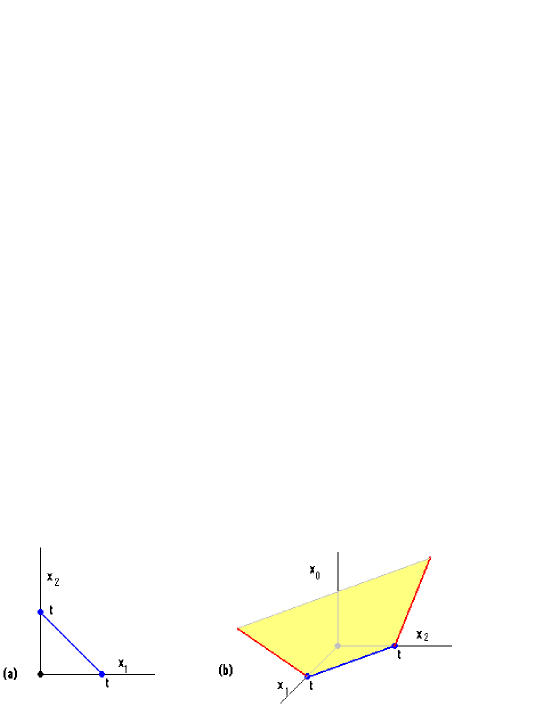
Figure 1: (a) Toric diagram of $P^{1},$ (b) Toric diagram of $\mathcal{O}\left(-2\right)\rightarrow P^{1}$

Recall also that the local space $NP^{1}$ is a toric complex surface capturing a natural $T^{2}$ fiber parameterized by the phases $\vartheta_{i}$ of the three complex variables $z_{0}$, $z_{1}$ and $z_{2}$, moded out by the $U\left(1\right)$ gauge symmetry of eq(3.3). The corresponding toric graph is given by a non compact real surface $B_{2}$,

$$x_{0}=\frac{1}{2}\left(x_{1}+x_{2}-t\right)\text{ },\qquad x_{i}\geq 0\text{ \ },$$ (3.7)

with a $T^{2}$ fiber.We have

$$NP^{1}=\cup_{p\in B_{2}}\left(\left\{p\right\}\times T_{p}^{2}\right),\qquad p=\left(x,y\right),$$ (3.8)

which we we denote formally as $T^{2}\times B_{2}$. Note that $NP^{1}$ is a toric surface, its boundary $\partial\left(NP^{1}\right)$ is also toric and is given by a $S_{x}^{1}$ fibration over the boundary real line

$$L=L_{1}\cup L_{2}\cup L_{0}$$ (3.9)

with

$$\left\{\begin{array}[]{c}L_{1}:x_{2}-2x_{0}-t=0,\qquad x_{1}=0\\ L_{2}:x_{1}-2x_{0}-t=0,\qquad x_{2}=0\\ L_{0}:x_{1}+x_{2}-t=0,\qquad x_{0}=0\end{array}\right..$$ (3.10)

The corresponding toric diagrams of eqs(3.7-3.10) are reported in figure (1a)-(1b).
For later use, it is interesting to consider the $S^{1}\times R$ fibration of $NP^{1}$ where the previous $T^{2}=S^{1}\times S^{1}$ fiber eq(3.8) gets replaced by $S^{1}\times R$. The second $S^{1}$ of $T^{2}$ has been decompactified to $R$. More details are given below.

3.1.2 $S^{1}\times R$ fibration of $NP^{1}$

In this setting, the local surface $NP^{1}$, and in general any smooth Calabi-Yau 2-fold, can be obtained by gluing together $C^{2}$ patches in a way that is consistent with Ricci-flatness. The geometry of $NP^{1}$ (and any Calabi-Yau 2-fold) is encoded in the one dimensional graph $\Gamma_{1}$ in the base that corresponds to the degeneration locus of the fibration. In the example of $NP^{1}$, shown on figure 2, we have two (bivalent) vertices $V_{1}$ and $V_{2}$. The edges $E_{1},$ $E_{2}$ and $E_{3}$ of the graph $\Gamma_{1}$ are oriented straight lines labeled by integers $p_{i}\in Z^{\ast}$ describing the shrinking 1-cycle $a_{i}\in H_{1}\left(S^{1}\right)$.

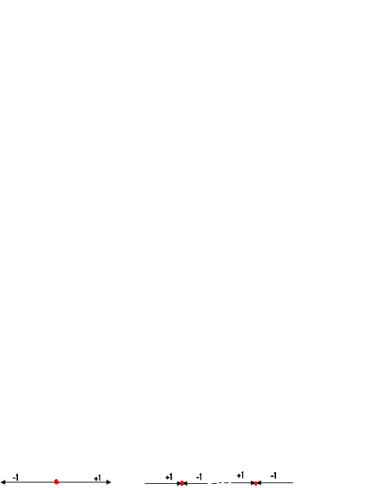
Figure 2: The graph of $S^{1}\times R$ fibration of $O\left(-2\right)\rightarrow P^{1}$. The local complex surface is built out of two $C^{2}$ patches with orientations as indicated in the figure. The transition functions correspond to a Z₂ transformation of the $S^{1}$ fibers as one goes from one patch to the other.

The condition of being a smooth Calabi-Yau is equivalent to the condition that on each vertex $V$, if we choose the edges to be outgoing with charges $p_{i}$, we must have

$$p_{1}+p_{2}=0.$$ (3.11)

For the case at hand, we have

$$\left\{\begin{array}[]{c}\text{vertex }V_{1}:\text{ }p_{11}+p_{12}=0\\ \text{vertex }V_{2}:\text{ }p_{21}+p_{22}=0\end{array}\right..$$ (3.12)

Changing the orientation on each edge $E_{i}$ corresponds to replacing $p_{i}\rightarrow-p_{i}$ which does not change the Calabi-Yau geometry. The graph of the $S^{1}\times R$ fibration of the local surface $NP^{1}$, which involves two open sets

$$U_{1}\left(z_{0},z_{1}\right)\simeq C^{2},\qquad U_{2}\left(z_{0},z_{2}\right)\simeq C^{2},$$ (3.13)

can be obtained as follows:
Let $z_{i}$ be local complex coordinates on $C^{2}$, $i=0,1$. In the patch $U_{1}\left(z_{0},z_{1}\right)$, the base of the $S^{1}$ fibration is the image of the moment map

$$r_{\alpha}=\left|z_{1}\right|^{2}-\left|z_{0}\right|^{2},$$ (3.14)

which reads in the patch $U_{2}\left(z_{0},z_{2}\right)$ as

$$r_{\alpha}=-\left|z_{2}\right|^{2}\ +\left|z_{0}\right|^{2}+t.$$

The non compact direction R is generated by $r_{\beta}=\mathop{\mathrm{I}m}\left(z_{0}z_{1}z_{2}\right)$. The special Lagrangian fiber is then generated by the action of the two “Hamiltonians” $r_{\alpha}$ and $r_{\beta}$ on $C^{2}$ via the standard symplectic form $\omega=i\left(dz_{0}\wedge d\overline{z}_{0}+dz_{1}\wedge d\overline{z}_{1}\right)$ on $C^{2}$ and the Poisson brackets $\partial z_{i}=\left\{r_{\alpha},z_{i}\right\}_{\omega}$. Note that the $S^{1}$ fiber is generated by the $U\left(1\right)$ action

$$e^{i\alpha r_{\alpha}}:\left(z_{0},z_{1}\right)\rightarrow\left(e^{-i\alpha}z_{0},e^{i\alpha}z_{1}\right),$$ (3.15)

which degenerates over $z_{0}=0=z_{1}$.

3.2 $NP^{2}$ as a planar geometry

3.2.1 $T^{3}$ fibration of $\mathcal{O}\left(-3\right)\rightarrow\mathbb{P}^{2}$

The toric diagram describing the complex projective surface $P^{2}$ is given by $T^{2}$ fibration over the dimension 2-simplex

$$B_{2}:x_{1}+x_{2}+x_{3}=t,$$ (3.16)

where $t$ is the $P^{2}$ Kahler parameter. $B_{2}$ is a finite equilateral triangle embedded in the $\mathbb{R}_{+}^{3}$ octant $\left(x_{1},x_{2},x_{3}\right)$. In the limit $t$ goes to zero, $B_{2}$ shrinks to the origin of the octant where lives a $P^{2}$ singularity.

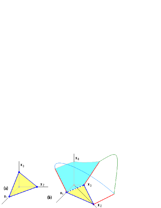
Figure 3: (a) Toric diagram of ${\small P}^{2}$. (b) Toric diagram of $\mathcal{O}\left(-3\right)\rightarrow P^{2}$ where divisors have been also represented.

In the case of the normal bundle $\mathcal{O}\left(-3\right)\rightarrow P^{2}$ viewed as a $T^{3}$ fibration over a real base $B_{3}$, the corresponding toric graph is given by,

$$x_{0}=\frac{1}{3}\left(x_{1}+x_{2}+x_{3}-t\right),\qquad x_{i}\geq 0.$$ (3.17)

with a $T^{3}$ fiber; i.e

$$NP^{2}\sim T^{3}\times B_{3}.$$ (3.18)

Note that $NP^{2}$ is toric and its boundary (divisor) is toric given by a $T^{2}$ fibration over the real surface

$$D=D_{0}\cup D_{1}\cup D_{3}\cup D_{4},$$ (3.19)

with,

$$\left\{\begin{array}[]{c}D_{0}:x_{1}+x_{2}+x_{3}-t=0,\qquad x_{0}=0\\ D_{1}:x_{2}+x_{3}-3x_{0}-t=0,\qquad x_{1}=0\\ D_{2}:x_{1}+x_{3}-3x_{0}-t=0,\qquad x_{2}=0\\ D_{3}:x_{1}+x_{2}-3x_{0}-t=0,\qquad x_{3}=0\end{array}\right.$$ (3.20)

The corresponding diagrams of eqs(3.17-3.20) are reported in figure (2a) and (2b).

3.2.2 $T^{2}\times R$ fibration of $NP^{2}$

The local surface $NP^{2}$, and in general any smooth toric Calabi-Yau 3-fold, can be obtained by gluing together $C^{3}$ patches in a way that is consistent with Ricci-flatness. The geometry of $NP^{2}$ (and any Calabi-Yau 3-fold) is encoded in a planar graph $\Gamma_{2}$ in the base that corresponds to the degeneration locus of the fibration. In the present example, shown on figure 3, we have three (trivalent) vertices $V_{1}$, $V_{2}$ and $V_{3}$. The edges $E_{i}\$of the graph $\Gamma_{2}$ are oriented straight lines labeled by integer 2-vectors

$$\mathbf{v}_{i}=\left(p_{i},q_{i}\right)\in Z^{2}$$ (3.21)

describing the shrinking 1-cycle $a_{i}\in H_{1}\left(T^{2}\right)$.

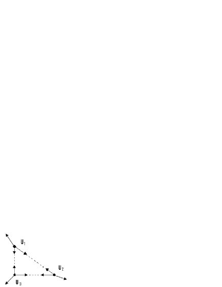
Figure 4: The graph of $T^{2}\times R$ fibration of $O\left(-3\right)\rightarrow P^{2}$. It is built out of three $C^{3}$ patches as indicated in the figure.

The condition of being a smooth toric Calabi-Yau is equivalent to the condition that on each vertex $V_{i}$, if we choose the edges to be outgoing with charges $\mathbf{v}_{i}$, we must have

$$\sum_{i=1}^{3}\mathbf{v}_{i}=0.$$ (3.22)

For the case at hand, we have

$$\left\{\begin{array}[]{c}\text{vertex }V_{1}:\text{ }\mathbf{v}_{11}+\mathbf{v}_{12}+\mathbf{v}_{13}=0\\ \text{vertex }V_{2}:\text{ }\mathbf{v}_{21}+\mathbf{v}_{22}+\mathbf{v}_{23}=0\\ \text{vertex }V_{3}:\text{ }\mathbf{v}_{31}+\mathbf{v}_{32}+\mathbf{v}_{33}=0\end{array}\right..$$ (3.23)

Changing the orientation on each edge $E_{i}$ corresponds to replacing $\mathbf{v}_{i}\rightarrow-\mathbf{v}_{i}$ which does not change the Calabi-Yau geometry. The graph of the $T^{2}\times\mathbb{R}$ fibration of the local surface $NP^{2}$ involves three patches

$$U_{1}\left(z_{0},z_{2},z_{3}\right)\simeq$$ , , ,

(3.24)

and can be obtained as follows:
In the local patch $U_{3}\left(z_{0},z_{1},z_{2}\right)$, the base of the $T^{2}$ fibration is the image of moment maps

$$\left\{\begin{array}[]{c}r_{\alpha}=-\left|z_{0}\right|^{2}+\left|z_{1}\right|^{2}\\ r_{\beta}=-\left|z_{0}\right|^{2}+\left|z_{2}\right|^{2}\end{array}\right..$$ (3.25)

From these relations, one can read the $U\left(1\right)\times U\left(1\right)$ charges $\left(\alpha,\beta\right)$ of the $z_{i}$ variables. We have for $z_{0}$, $z_{1}$ and $z_{2}$ respectively

$$\mathbf{v}_{11}=\left(-1,-1\right)$$ , ,

(3.26)

Similarly, we write down the $r_{\alpha}$ and $r_{\beta}$ maps in the patch $U_{2}\left(z_{0},z_{1},z_{3}\right)$ and so the corresponding $\mathbf{v}_{2i}$ vectors. We have:

$$r_{\alpha}=-\left|z_{0}\right|^{2}+\left|z_{1}\right|^{2}$$ ,

,

(3.27)

and

$$\left\{\begin{array}[]{c}\mathbf{v}_{21}=\left(-1,2\right)\\ \mathbf{v}_{22}=\left(1,-1\right)\\ \mathbf{v}_{23}=\left(0,-1\right)\end{array},\qquad\mathbf{v}_{21}+\mathbf{v}_{22}+\mathbf{v}_{23}=0\right.$$ (3.28)

An analogous analysis for the local patch $U_{1}\left(z_{0},z_{2},z_{3}\right)$ leads to:

$$r_{\alpha}=2\left|z_{0}\right|^{2}-\left|z_{2}\right|^{2}-\left|z_{3}\right|^{2}+t$$ ,

,

(3.29)

and

$$\left\{\begin{array}[]{c}\mathbf{v}_{31}=\left(2,-1\right)\\ \mathbf{v}_{32}=\left(-1,1\right)\\ \mathbf{v}_{33}=\left(-1,0\right)\end{array},\qquad\mathbf{v}_{31}+\mathbf{v}_{32}+\mathbf{v}_{33}=0\right.$$ (3.30)

The non compact direction $R$ is generated by $r_{\gamma}=\mathop{\mathrm{I}m}\left(z_{0}z_{1}z_{2}z_{3}\right)$. The special Lagrangian fiber is then generated by the action of the three “Hamiltonians” $r_{\alpha},$ $r_{\beta}$ and $r_{\gamma}$ on $C^{3}$ via the standard symplectic form $\omega=i\sum_{i}dz_{i}\wedge d\overline{z}_{i}$ and the Poisson bracket $\partial z_{i}=\left\{r,z_{i}\right\}_{\omega}$. Note that the $T^{2}$ fiber generated by $U\left(1\right)\times U\left(1\right)$ action,

$$e^{i\alpha r_{\alpha}+i\beta r_{\beta}}:\left(z_{0},z_{1},z_{2}\right)\rightarrow\left(e^{-i\left(\alpha+\beta\right)}z_{0},e^{i\alpha}z_{1},e^{i\beta}z_{2}\right),$$ (3.31)

degenerates over $z_{0}=0=z_{1}=z_{2}$.

3.3 $NP^{3}$ as a non planar geometry

3.3.1 $T^{4}$ fibration of $NP^{3}$

The previous analysis extends naturally to the present case. The toric diagram of the complex projective space $P^{3}$ is given by $T^{3}$ fibration over the 3-simplex

$$B_{3}:x_{1}+x_{2}+x_{3}+x_{4}=t.$$ (3.32)

The latter is a finite tetrahedron (a pyramid) embedded in $R_{+}^{4}$ parameterized by $\left(x_{1},x_{2},x_{3},x_{4}\right)$ which, in the limit $t$ goes to zero, shrinks to the origin of $R_{+}^{4}$ where lives a $P^{3}$ singularity.

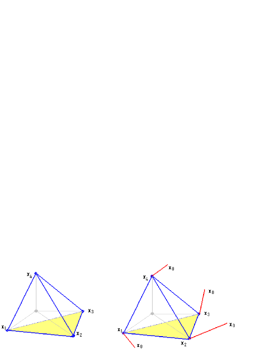
Figure 5: On left: toric diagram of P³. On right toric diagram of $\mathcal{O}\left(-4\right)\rightarrow P^{3}$.

The toric graph of the normal bundle $NP^{3}$ viewed as a $T^{4}$ fibration over a real base $B_{4}$ is given by

$$x_{0}=\frac{1}{4}\left(x_{1}+x_{2}+x_{3}+x_{4}-t\right),\qquad x_{i}\geq 0.$$ (3.33)

with a $T^{4}$ fiber. Notice that $NP^{3}$ is toric; its boundary is also toric and is given by an $T^{3}$ fibration over the real 3-spaces $D_{i}$:

$$\left\{\begin{array}[]{c}D_{0}:x_{1}+x_{2}+x_{3}+x_{4}-t=0,\qquad x_{0}=0\\ D_{1}:x_{2}+x_{3}+x_{4}-3x_{0}-t=0,\qquad x_{1}=0\\ D_{2}:x_{1}+x_{3}+x_{4}-3x_{0}-t=0,\qquad x_{2}=0\\ D_{3}:x_{1}+x_{2}+x_{4}-3x_{0}-t=0,\qquad x_{3}=0\\ D_{4}:x_{1}+x_{2}+x_{3}-3x_{0}-t=0,\qquad x_{4}=0\end{array}\right.$$ (3.34)

The toric diagrams of $P^{3}$ and $NP^{3}$ are reported in figure (3a) and (3b).

3.3.2 $T^{3}\times R$ fibration of $NP^{3}$

The local surface $NP^{3}$ and in general any smooth Calabi-Yau 4-fold can be obtained by gluing together $C^{4}$ patches in a way that is consistent with Ricci-flatness. For each $C^{4}$ patch, we have four outgoing 3-vectors adding to zero as indicated on the example given by figure 6,

Figure 6: The graph of $C^{4}$

The geometry of full $NP^{3}$ is then encoded in a non planar 3-dimensional graph $\Gamma_{3}$ in the base that corresponds to the degeneration locus of the fibration $T^{3}\times R$. In the present example, shown on figure 7, we have four (tetravalent) vertices $V_{1}$, $V_{2}$, $V_{3}$ and $V_{4}$. The edges $E_{i}\$of the graph $\Gamma_{3}$ are oriented straight lines labeled by integer 3-vectors

$$\mathbf{v}_{i}=\left(p_{i},q_{i},s_{i}\right)\in Z^{3},$$ (3.35)

describing the shrinking 1-cycle $a_{i}\in H_{1}\left(T^{3}\right)$.

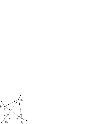
Figure 7: The graph of $T^{3}\times R$ fibration of $O\left(-4\right)\rightarrow P^{3}$. It is built out of four $C^{4}$ patches as in the figure.

The condition of being a smooth toric Calabi-Yau is equivalent to the condition that on each vertex $V_{i}$, if we choose the edges to be outgoing with charges $\mathbf{v}_{i}$, we must have

$$\sum_{i=1}^{4}\mathbf{v}_{i}=0.$$ (3.36)

For the case at hand, we have

$$\left\{\begin{array}[]{c}\text{vertex }V_{1}:\text{ }\mathbf{v}_{11}+\mathbf{v}_{12}+\mathbf{v}_{13}+\mathbf{v}_{14}=0\\ \text{vertex }V_{2}:\text{ }\mathbf{v}_{21}+\mathbf{v}_{22}+\mathbf{v}_{23}+\mathbf{v}_{24}=0\\ \text{vertex }V_{3}:\text{ }\mathbf{v}_{31}+\mathbf{v}_{32}+\mathbf{v}_{33}+\mathbf{v}_{34}=0\\ \text{vertex }V_{4}:\text{ }\mathbf{v}_{41}+\mathbf{v}_{42}+\mathbf{v}_{43}+\mathbf{v}_{44}=0\end{array}\right..$$ (3.37)

As we see, changing the orientation on each edge $E_{i}$ corresponds to replacing $\mathbf{v}_{i}\rightarrow-\mathbf{v}_{i}$ which does not change the Calabi-Yau geometry. The graph of the $T^{3}\times R$ fibration of  $NP^{3}$ involves four patches

$$U_{1}\left(z_{0},z_{2},z_{3},z_{4}\right)\simeq$$ , ,

, ,

(3.38)

and can be obtained as follows:
In the local patch $U_{4}\left(z_{0},z_{1},z_{2},z_{3}\right)$, the base of the $T^{3}$ fibration is the image of the moment maps

$$\left\{\begin{array}[]{c}r_{\alpha}=-\left|z_{0}\right|^{2}+\left|z_{1}\right|^{2},\\ r_{\beta}=-\left|z_{0}\right|^{2}+\left|z_{2}\right|^{2},\\ r_{\gamma}=-\left|z_{0}\right|^{2}+\left|z_{3}\right|^{2}.\end{array}\right.$$ (3.39)

From these relations, one can read the $U^{3}\left(1\right)$ charges $\left(\alpha,\beta,\gamma\right)$ of the $z_{i}$ variables. We have, see also the corresponding figure,

$$\left\{\begin{tabular}[]{lll}$\mathbf{v}_{41}$&$=$&$\left(-1,-1,-1\right)$\\ $\mathbf{v}_{42}$&$=$&$\left(1,0,0\right)$\\ $\mathbf{v}_{43}$&$=$&$\left(0,1,0\right)$\\ $\mathbf{v}_{44}$&$=$&$\left(0,0,1\right)$\end{tabular}\ ,\qquad\mathbf{v}_{41}+\mathbf{v}_{42}+\mathbf{v}_{43}+\mathbf{v}_{44}=0\right..$$ (3.40)

In the local patch $U_{1}\left(z_{0},z_{2},z_{3},z_{4}\right)$, the maps as well as the corresponding $\mathbf{v}_{1i}$ vectors are:

$$\left\{\begin{tabular}[]{lll}$r_{\alpha}$&$=$&$3\left|z_{0}\right|^{2}-\left|z_{2}\right|^{2}-\left|z_{3}\right|^{2}-\left|z_{4}\right|^{2}+t$\\ $r_{\beta}$&$=$&$-\left|z_{0}\right|^{2}+\left|z_{2}\right|^{2}$\\ $r_{\gamma}$&$=$&$-\left|z_{0}\right|^{2}+\left|z_{3}\right|^{2}$\end{tabular}\ \right.$$ (3.44)

$$\left\{\begin{tabular}[]{lll}$\mathbf{v}_{11}$&$=$&$\left(3,-1,-1\right)$\\ $\mathbf{v}_{12}$&$=$&$\left(-1,1,0\right)$\\ $\mathbf{v}_{13}$&$=$&$\left(-1,0,1\right)$\\ $\mathbf{v}_{14}$&$=$&$\left(-1,0,0\right)$\end{tabular}\ ,\qquad\mathbf{v}_{11}+\mathbf{v}_{12}+\mathbf{v}_{13}+\mathbf{v}_{14}=0\right.$$ (3.49)

Similarly, we can write down the hamiltonian maps and the vectors $\mathbf{v}_{2i}$ in the patch $U_{2}\left(z_{0},z_{1},z_{3},z_{4}\right)$. We have,

$$\left\{\begin{tabular}[]{llll}$r_{\alpha}$&$=$&$-\left|z_{0}\right|^{2}+\left|z_{1}\right|^{2}$&$,$\\ $r_{\beta}$&$=$&$3\left|z_{0}\right|^{2}-\left|z_{1}\right|^{2}-\left|z_{3}\right|^{2}-\left|z_{4}\right|^{2}+t$&$,$\\ $r_{\gamma}$&$=$&$-\left|z_{0}\right|^{2}+\left|z_{3}\right|^{2}$&$.$\end{tabular}\ \right.$$ (3.53)

$$\left\{\begin{tabular}[]{lll}$\mathbf{v}_{21}$&$=$&$\left(-1,3,-1\right)$\\ $\mathbf{v}_{22}$&$=$&$\left(1,-1,0\right)$\\ $\mathbf{v}_{23}$&$=$&$\left(0,-1,1\right)$\\ $\mathbf{v}_{24}$&$=$&$\left(0,-1,0\right)$\end{tabular}\ ,\qquad\mathbf{v}_{21}+\mathbf{v}_{22}+\mathbf{v}_{23}+\mathbf{v}_{24}=0\right.$$ (3.58)

We also have for the local patch $U_{3}\left(z_{0},z_{1},z_{2},z_{4}\right)$:

$$\left\{\begin{tabular}[]{llll}$r_{\alpha}$&$=$&$-\left|z_{0}\right|^{2}+\left|z_{1}\right|^{2}$&$,$\\ $r_{\beta}$&$=$&$-\left|z_{0}\right|^{2}+\left|z_{2}\right|^{2}$&$,$\\ $r_{\gamma}$&$=$&$3\left|z_{0}\right|^{2}-\left|z_{1}\right|^{2}-\left|z_{2}\right|^{2}-\left|z_{4}\right|^{2}+t$&$.$\end{tabular}\ \right.$$ (3.62)

$$\left\{\begin{tabular}[]{lll}$\mathbf{v}_{31}$&$=$&$\left(-1,-1,3\right)$\\ $\mathbf{v}_{32}$&$=$&$\left(1,0,-1\right)$\\ $\mathbf{v}_{33}$&$=$&$\left(0,1,-1\right)$\\ $\mathbf{v}_{34}$&$=$&$\left(0,0,-1\right)$\end{tabular}\ ,\qquad\mathbf{v}_{31}+\mathbf{v}_{32}+\mathbf{v}_{33}+\mathbf{v}_{34}=0\right..$$ (3.67)

The non compact direction $R$ is generated by $r_{\delta}=\mathop{\mathrm{I}m}\left(z_{0}z_{1}z_{2}z_{3}z_{4}\right)$. This analysis generalizes immediately to $\mathcal{O}\left(-n\right)\rightarrow P^{n-1}$ with $n>4$.

4 Local degenerate elliptic curve

Always interested in the study of local Calabi-Yau threefold, we focus in this section on the particular local degenerate elliptic curve,

$$H_{3}=\mathcal{O}(+3)\oplus\mathcal{O}(-3)\rightarrow E^{\left(t,\infty\right)}$$ , .

(4.1)

The elliptic curve can be generally denoted as $E^{\left(t,\mu\right)}$ as it has one Kahler parameter $t$ and one complex parameter $\mu$. Below, we will consider the limit $\mu\rightarrow\infty$ so that $E^{\left(t,\infty\right)}$ can be identified with $E=P_{1}^{1}\cup P_{2}^{1}\cup P_{3}^{1}$ with matrix intersection (2.21)

4.1 Embedding local $E^{\left(t,\infty\right)}$ in NP³

First, notice that there exist various ways to describe the above local elliptic curve $E^{\left(t,\infty\right)}$ in $NP^{3}$. One way to do is to think about $NP^{3}$ as a fibration of the compact line bundle $\mathcal{O}\left(+3\right)$ over the local complex surface $X_{2}=\mathcal{O}\left(-3\right)\rightarrow E^{\left(t,\infty\right)}$. In this case, the base $E^{\left(t,\infty\right)}$ ($E$ for short) is a toric line realized by the special toric curve $P_{1}^{1}\cup P_{2}^{1}\cup P_{3}^{1}$. Then, $E$ is the toric boundary of the complex projective plane $P^{2}$,

$$E=\partial\left(P^{2}\right).$$ (4.2)

So, the toric graph of the compact part of $H_{3}$ consists of three intersecting triangles forming the boundary surface of a hollow tetrahedron. The toric graph of the shrinking 1-cycles of $\mathcal{O}\left(+3\right)\rightarrow X_{2}$ is given by figure 11.

Figure 8: Non planar toric web-diagram of  $\mathcal{O}\left(+3\right)\oplus\mathcal{O}\left(-3\right)\rightarrow E^{\left(t,\infty\right)}$. This is a toric CY3 divisor of the four dimension complex Kahler manifold $\mathcal{O}\left(+3\right)\oplus\mathcal{O}\left(-3\right)\rightarrow P^{2}$  The hollow triangle ABC refers to the degenerate elliptic curve $E^{\left(t,\infty\right)}$. The full triangles ABD, ZCD, BCD refer to the three other projective planes.

This non standard Calabi-Yau threefold $X_{3}=\mathcal{O}\left(+3\right)\oplus X_{2}$, with $X_{2}=\mathcal{O}\left(-3\right)\rightarrow E$ involves non planar toric graphs.
Because of the nature of the base $E$ which is built out of the three intersecting projective lines $P_{1}^{1},$ $P_{2}^{1},$ $P_{3}^{1}$ of $P^{2}$ and because of the $\mathcal{O}\left(+3\right)$ fibration, the toric data of the variety $X_{3}$ can be deduced from that of the normal bundle of the complex three dimension weighted projective space W$\mathbb{P}_{1113}^{3}$.
An other way to thinking about $X_{3}$ is

$$X_{3}=\mathcal{O}\left(-3\right)\rightarrow X_{2}^{\prime},$$ (4.3)

with

$$X_{2}^{\prime}=\mathcal{O}\left(+3\right)\rightarrow E.$$ (4.4)

describing the toric boundary surface of the complex dimension three weighted projective space;  i.e

$$X_{2}^{\prime}\subset WP_{1,1,1,3}^{3}$$ (4.5)

As we know $WP_{1,1,1,3}^{3}$, which roughly looks like $P^{3}$, has a non planar toric graph with:
- Four faces (divisors) F₁, F₂, F₃ and F₄,
- Six edges E₁, E₂, E₃, E₄, E₅, E₆; and
- Four vertices V₁, V₂, V₃ and V₄.
By supplying the $\mathcal{O}\left(-3\right)$ fibration, the toric threefold $X_{3}$ can be viewed as a local Calabi-Yau submanifold of a complex four dimension Kahler manifold $Y_{4}$; that is:

$$X_{3}\subset Y_{4}:$$ .

(4.6)

In the framework of the topological string setting, the 4- vertices are described by local patches $U_{i}\simeq$ $C^{4}$,

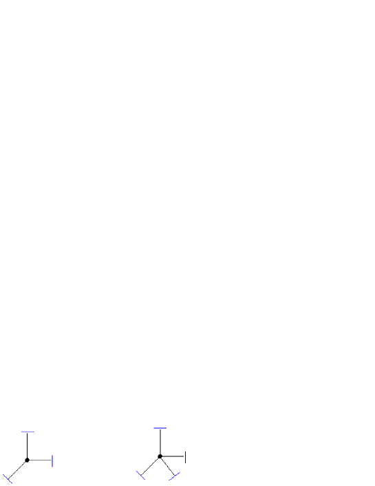
Figure 9: On left the graph of topological 3-vertex where each leg ends on a lagrangian submanifold. On right, we have the 4-vertex analog.

We will address this question with some details later on; but before that we first focus on the toric data of

$$\mathcal{O}\left(-3\right)\rightarrow WP_{1,1,1,3}^{3}$$ (4.7)

and its toric submanifold

$$\mathcal{O}\left(-3\right)\rightarrow\partial\left(WP_{1,1,1,3}^{3}\right).$$ (4.8)

Generally, a toric CY4- fold with local patches $C^{4}$ parameterized by complex coordinates $\left\{w_{i}\right\}$ has the natural toric (trivial) fibration

$$B_{4}\times T^{4},$$ (4.9)

with real base $B_{4}\subset R^{4}$ and a Kahler form $J=i\sum_{i,j=1}^{4}\ dw_{i}\wedge d\overline{w}_{i}$. This form splits in the $\left(\left|w_{i}\right|^{2},\vartheta_{i}\right)$ polar coordinates as

$$\mathbf{J}=\sum_{i=1}^{4}d\rho_{i}^{2}\wedge d\vartheta_{i}$$ , , .

(4.10)

A Lagrangian submanifold $L_{4}$ of $C^{4}$ is a real 4-dimensional subspace satisfying the usual property,

$$\mathbf{J}\mid_{L_{4}}=0.$$ (4.11)

By using eq(4.10), we see that this constraint eq can be solved in different ways; for instance by taking $\rho_{i}^{2}$ = constant ($d\rho_{i}^{2}=0$) or by setting $\vartheta_{i}$ = constant ($d\vartheta_{i}=0$).
One can also build special Lagrangian submanifolds $\mathcal{L}$ satisfying, in addition to eq(4.11), the constraint eq

$$\left(\mathop{\mathrm{I}m}\Omega\right)\mid_{\mathcal{L}}=0$$ (4.12)

where $\Omega$ is the usual holomorphic $\left(4,0\right)$ form.
In the present study, we are interested in the $T^{2}\times R$ special Lagrangian fibration of the toric Calabi-Yau threefold $\mathcal{O}\left(-3\right)\rightarrow\partial\left(WP_{1,1,1,3}^{3}\right)$. This fibration extends to a $T^{3}\times R$ fibration of the ambient space $\mathcal{O}\left(-3\right)\rightarrow WP_{1,1,1,3}^{3}$.

4.1.1 Toric graph of $\mathcal{O}\left(-3\right)\rightarrow\partial\left(WP_{1,1,1,3}^{3}\right)$

The toric graph of the Calabi-Yau threefold $\mathcal{O}\left(-3\right)\rightarrow\partial\left(WP_{1,1,1,3}^{3}\right)$ can be determined from the graph of the manifold $\mathcal{O}\left(-3\right)\rightarrow WP_{1,1,1,3}^{3}$. Both of these Kahler manifolds are realized as a complex 3- and  complex 4- dimension toric hypersurfaces embedded in $C^{5}$. For the case of $\mathcal{O}\left(-3\right)\rightarrow WP_{1,1,1,3}^{3}$, the defining equation is given by

$$\sum_{i=1}^{3}|w_{i}|^{2}+3|w_{4}|^{2}-3|w_{0}|^{2}=t.$$ (4.13)

For $O\left(-3\right)\rightarrow\partial\left(WP_{1,1,1,3}^{3}\right)$ we have, in addition to 4.13, the extra condition

$$w_{1}w_{2}w_{3}=0.$$ (4.14)

As mentioned earlier, eq(4.14) may be solved in three ways; either by $w_{1}=0$ whatever $w_{2}$ and $w_{3}$ are, or by taking$\ w_{2}=0$ or again by setting $w_{3}=0$. Notice that both eqs(4.13-4.14) are invariant under the $U\left(1\right)$ transformations of the complex variables

$$w_{j}\equiv e^{i\alpha q_{j}}w_{j}.$$ (4.15)

Notice also that the sum of the $U\left(1\right)$ charges

$$\left(q_{0},q_{1},q_{2},q_{3},q_{4}\right)=\left(-3,1,1,1,3\right)$$ (4.16)

is non zero;

$$\sum_{j=0}^{4}q_{j}=3.$$ (4.17)

It shows that $O\left(-3\right)\rightarrow WP_{1,1,1,3}^{3}$ is not a Calabi-Yau 4-fold; while $\mathcal{O}\left(-3\right)\rightarrow\partial\left(WP_{1,1,1,3}^{3}\right)$ is a Calabi-Yau threefold. To handle the relations (4.13-4.14), we shall proceed as follows: First deal with eq(4.13) and then implement the constraint eq(4.14).

4.1.2 Analysis of eq(4.13)

We start from equation $\sum_{i=1}^{3}|w_{i}|^{2}+3|w_{4}|^{2}-3|w_{0}|^{2}=t$ and solve it in four different ways according to which set of variables is used. We have the following $C^{4}$ patches:

$$U_{1}=U_{1}\left(w_{2},w_{3},w_{4},w_{0}\right)\$$ ,

,

,

.

(4.18)

On the coordinate patch $U_{1}$, the Kahler manifold $\mathcal{O}\left(-3\right)\rightarrow WP_{1,1,1,3}^{3}$ is described by the codimension one hypersurface of $C^{5}$,

$$|w_{4}|^{2}=\frac{t}{3}+|w_{0}|^{2}-\frac{1}{3}\sum_{i=1}^{3}|w_{i}|^{2}.$$ (4.19)

Similarly, we have for the patch $U_{1}$, $U_{2}$ and $U_{3}$ the following relations,

$$|w_{1}|^{2} = t+3|w_{0}|^{2}-|w_{2}|^{2}-|w_{3}|^{2}-3|w_{4}|^{2},$$

$$|w_{2}|^{2} = t+3|w_{0}|^{2}-|w_{1}|^{2}-|w_{3}|^{2}-3|w_{4}|^{2},$$ (4.20)

$$|w_{3}|^{2} = t+3|w_{0}|^{2}-|w_{1}|^{2}-|w_{2}|^{2}-3|w_{4}|^{2}.$$

Each one of the local patches $U_{i}$ is isomorphic to C⁴. To get the toric graph of the shrinking 2- cycles, we have to first identify the hamiltonians of the $T^{3}\times R$ fibration of $\mathcal{O}\left(-3\right)\rightarrow WP_{1,1,1,3}^{3}$.

4.1.3 Hamiltonians on the U₄ patch

Following the same method, we have used in subsection 2.2 concerning $T^{3}\times R$ fibration of the 4- fold $\mathcal{O}\left(-4\right)\rightarrow P^{3}$, see eqs(4.13-4.14), the hamiltonians

$$H_{\alpha},\quad H_{\beta},\quad H_{\gamma},\quad H_{\delta},$$ (4.21)

generating of the $T^{3}\times R$ special Lagrangian fibration depends on the local patches we are sitting on. We have:

Local patch $w_{4}=f_{4}\left(w_{i}\right)$:  
On the patch $U_{4}\left(w_{1},w_{2},w_{3},w_{0}\right)$ of the 4- fold $\mathcal{O}\left(-3\right)\rightarrow WP_{1,1,1,3}^{3}$ where $w_{4}$ is solved in terms of the four complex variables $\left(w_{1},w_{2},w_{3},w_{0}\right)$ as shown above, the three projective variables $w_{1},w_{2},w_{3}$ play a symmetric role. So the three hamiltonians

$$H_{\alpha}=H_{\alpha}^{\left(4\right)},\quad H_{\beta}=H_{\beta}^{\left(4\right)},\quad H_{\gamma}=H_{\gamma}^{\left(4\right)},$$ (4.22)

generating the 2-cycles of $T^{3}$ can be written as follows:

$$U_{4}:\left\{\begin{array}[]{c}\begin{array}[]{c}H_{\alpha}^{\left(4\right)}=|w_{1}|^{2}-|w_{0}|^{2}\\ H_{\beta}^{\left(4\right)}=|w_{2}|^{2}-|w_{0}|^{2}\\ H_{\gamma}^{\left(4\right)}=|w_{3}|^{2}-|w_{0}|^{2}\end{array}\\ \mathrm{H}_{\delta}^{\left(4\right)}=\mathop{\mathrm{I}m}w_{1}w_{2}w_{3}w_{4}w_{0}\end{array}\right..$$ (4.23)

From these relations, we can write down the outgoing (”momentum”) vectors

$$v_{1}^{\left(4\right)},\quad v_{2}^{\left(4\right)},\quad v_{3}^{\left(4\right)},\quad v_{0}^{\left(4\right)},$$ (4.24)

describing the shrinking 1-cycles on the four edges of the vertex $C^{4}$ associated with the toric graph of the $U_{4}$ patch. We have,

$$v_{1}^{\left(4\right)}=\left(1,0,0\right),$$ .

Before proceeding further, notice the two following:
(i) the sum of the $v_{i}^{\left(4\right)}$ momenta add exactly to zero

$$\sum_{i=0}^{3}v_{i}^{\left(4\right)}=\left(0,0,0\right)$$ (4.25)

This property seems a little bit strange as one expects something different from zero since the 4- fold $\mathcal{O}\left(-3\right)\rightarrow WP_{1,1,1,3}^{3}$ is not a Calabi-Yau manifold. We will turn later on to this point and show that for the other vertices the sum of momentum vectors is non zero.
(ii) Imposing the condition

$$w_{1}w_{2}w_{3}=0,$$ (4.26)

on the patch $U_{4}$ and solving it in three ways as $w_{1}=0$, $w_{2}w_{3}\neq 0$, or $w_{2}=0$, $w_{1}w_{3}\neq 0$ or again $w_{3}=0$, $w_{2}w_{1}\neq 0$, we discover that $U_{4}$ can be split into complex 3- dimension local patches $U_{4i}$ equivalent to $C^{3}$. These are given by,

$$U_{41} = U_{41}\left(w_{2},w_{3},w_{0}\right),$$

$$U_{42} = U_{42}\left(w_{1},w_{3},w_{0}\right),$$ (4.27)

$$U_{43} = U_{43}\left(w_{1},w_{2},w_{0}\right),$$

where, for instance, the subindex on $U_{41}$ refers to the fact that on this local patch we have $w_{4}=f\left(w_{i}\right)$ and $w_{1}=0$. The hamiltonians generating the 1- cycles of the $T^{2}\times R$ fibration read respectively as follows:

$$U_{41}\ : \left\{\begin{array}[]{c}H_{\beta}^{\left(41\right)}=|w_{2}|^{2}-|w_{0}|^{2}\\ H_{\gamma}^{\left(41\right)}=|w_{3}|^{2}-|w_{0}|^{2}\end{array}\right.,\quad$$ (4.30)

$$U_{42} : \left\{\begin{array}[]{c}H_{\alpha}^{\left(42\right)}=|w_{1}|^{2}-|w_{0}|^{2}\\ H_{\gamma}^{\left(42\right)}=|w_{3}|^{2}-|w_{0}|^{2}\end{array}\right.,\quad$$ (4.33)

$$U_{43} : \left\{\begin{array}[]{c}H_{\alpha}^{\left(43\right)}=|w_{1}|^{2}-|w_{0}|^{2}\\ H_{\beta}^{\left(43\right)}=|w_{2}|^{2}-|w_{0}|^{2}\end{array}\right.$$ (4.36)

From these relations, we can write down the momentum vectors of the shrinking 1- cycles of the $T^{2}\times R$ fibration. We have the following projections:

$$U_{41}:$$

(4.37)

Note that on all $U_{4i}$ patches, we have

$$\mathrm{H}_{\delta}^{\left(4i\right)}=0$$ (4.38)

and the sums $\sum_{j}v_{j}^{\left(4i\right)}$ add exactly to zero.

4.2 More on Hamiltonians

Local patch $U_{1}$:  
On the local patch $U_{1}\left(w_{2},w_{3},w_{4},w_{0}\right)$, the variable $w_{1}$ is expressed as $f_{1}\left(w_{2},w_{3},w_{4},w_{0}\right)$. The method is quite similar to the one used above. The hamiltonians generating the cycles of the $T^{3}\times R$ of the $U_{1}$ patch of the complex four dimension space $\mathcal{O}\left(-3\right)\rightarrow WP_{1,1,1,3}^{3}$ read as follows:

$$U_{1}\ :\left\{\begin{array}[]{c}H_{\alpha}^{\left(1\right)}=-|w_{2}|^{2}-|w_{3}|^{2}-3|w_{4}|^{2}+2|w_{0}|^{2}+t\\ H_{\beta}^{\left(1\right)}=|w_{2}|^{2}-|w_{0}|^{2}\text{ \ \ \ \ \ \ \ \ \ \ \ \ \ \ \ \ \ \ \ \ \ \ \ \ \ \ \ \ \ \ \ \ \ }\\ H_{\gamma}^{\left(1\right)}=|w_{3}|^{2}-|w_{0}|^{2}\text{ \ \ \ \ \ \ \ \ \ \ \ \ \ \ \ \ \ \ \ \ \ \ \ \ \ \ \ \ \ \ \ \ \ \ }\end{array}\right.,$$ (4.39)

where we have substituted $w_{1}$ by its expression $f_{1}\left(w_{2},w_{3},w_{4},w_{0}\right)$. The momentum vectors

$$v_{i}^{\left(1\right)},\quad i=0,1,2,3,$$ (4.40)

associated with the shrinking 2- cycles of the special Lagrangian fibration are given by:

$$v_{1}^{\left(1\right)}=\left(-1,1,0\right)$$ , ,

, .

(4.41)

Note that, contrary to the previous case, the sum of these vectors is non zero.

$$\sum_{i=0}^{3}v_{i}^{\left(1\right)}=\left(-3,0,0\right).$$ (4.42)

This property was expected and it reflects just the fact that complex 4-dimension $\mathcal{O}\left(-3\right)\rightarrow WP_{1,1,1,3}^{3}$ described by the hypersurface,

$$\sum_{i=1}^{3}|w_{i}|^{2}+3|w_{4}|^{2}-3|w_{0}|^{2}=t,$$ (4.43)

is not a Calabi-Yau 4-fold. Moreover solving the condition $w_{1}w_{2}w_{3}=0$ on the patch $U_{1}$ as

$$w_{2}=0$$ or ,

(4.44)

we find that $U_{1}$ can be split into two local patches $U_{1i}$ equivalent to $C^{3}$. These are given by,

$$U_{12}=U_{12}\left(w_{3},w_{4},w_{0}\right)$$ ,

.

(4.45)

Then, the corresponding hamiltonians $H_{\alpha}^{\left(12\right)},H_{\gamma}^{\left(12\right)}$ for the case $w_{2}=0$ and $H_{\alpha}^{\left(13\right)},$ $H_{\beta}^{\left(13\right)}$ for $w_{3}=0$, read as follows:

$$U_{12}\ : \left\{\begin{array}[]{c}H_{\alpha}^{\left(12\right)}=-|w_{3}|^{2}-3|w_{4}|^{2}+2|w_{0}|^{2}+t\\ H_{\gamma}^{\left(12\right)}=|w_{3}|^{2}-|w_{0}|^{2}\text{\qquad\qquad\qquad\ \ \ }\end{array}\right.$$ (4.48)

$$U_{13}\ : \left\{\begin{array}[]{c}H_{\alpha}^{\left(13\right)}=-|w_{2}|^{2}-3|w_{4}|^{2}+2|w_{0}|^{2}+t\\ H_{\beta}^{\left(13\right)}=|w_{2}|^{2}-|w_{0}|^{2}\text{ \ \ \ \ \ \ \ \ \ \ \ \ \ \ \ \ \ \ \ \ \ }\end{array}\right..$$ (4.51)

and they generate 1-cycles of the $T^{2}\times R$ ,. The vector momenta of the shrinking cycles are

$$\ v_{3}^{\left(12\right)} = \left(-1,\mathrm{\ast},1\right),\quad v_{4}^{\left(12\right)}=\left(-3,\mathrm{\ast},0\right),\quad v_{0}^{\left(12\right)}=\left(2,\mathrm{\ast},-1\right),$$

$$v_{2}^{\left(13\right)} = \left(-1,1,\mathrm{\ast}\right),\quad v_{4}^{\left(13\right)}=\left(-3,0,\mathrm{\ast}\right),\quad v_{0}^{\left(13\right)}=\left(2,-1,\mathrm{\ast}\right).$$ (4.52)

Local patch $U_{2}$:
Similarly, the hamiltonians generating the cycles of the $T^{3}\times R$ fibration on the $U_{2}=U_{2}\left(w_{1},w_{3},w_{4},w_{0}\right)$ patch, with $w_{2}=f_{2}\left(w_{i}\right)$, read as follows:

$$U_{2}:\left\{\begin{tabular}[]{lll}$H_{\alpha}^{\left(1\right)}$&$=$&$|w_{1}|^{2}-|w_{0}|^{2}$\\ $H_{\beta}^{\left(1\right)}$&$=$&$t+2|w_{0}|^{2}-|w_{1}|^{2}-|w_{3}|^{2}-3|w_{4}|^{2}$\\ $H_{\gamma}^{\left(1\right)}$&$=$&$|w_{3}|^{2}-|w_{0}|^{2}$\end{tabular}\ \right..$$ (4.53)

The vectors

$$v_{0}^{\left(2\right)},\text{ \ }v_{1}^{\left(2\right)},\text{ \ }v_{2}^{\left(2\right)},\text{ \ }v_{3}^{\left(2\right)},\text{ }$$ (4.54)

associated with the shrinking 1-cycles of these hamiltonians are

$$v_{1}^{\left(2\right)} = \left(1,-1,0\right),\quad v_{2}^{\left(2\right)}=\left(0,-1,1\right),$$

$$v_{3}^{\left(2\right)} = \left(0,-3,0\right),\quad v_{0}^{\left(2\right)}=\left(-1,2,-1\right).$$ (4.55)

Here also, the sum of the $v_{i}^{\left(2\right)}$s is non zero

$$\sum_{i=0}^{3}v_{i}^{\left(2\right)}=\left(0,-3,0\right).$$ (4.56)

Local patch $U_{3}$:
In this case, the Hamiltonians read as,

$$U_{3}\ :\left\{\begin{tabular}[]{lll}$H_{\alpha}^{\left(1\right)}$&$=$&$|w_{1}|^{2}-|w_{0}|^{2}$\\ $H_{\beta}^{\left(1\right)}$&$=$&$|w_{2}|^{2}-|w_{0}|^{2}$\\ $H_{\gamma}^{\left(1\right)}$&$=$&$t+2|w_{0}|^{2}-|w_{1}|^{2}-|w_{2}|^{2}-3|w_{4}|^{2}$\end{tabular}\right.$$ (4.57)

and the associated vectors $v_{i}^{\left(3\right)}$ take the form:

$$v_{1}^{\left(3\right)} = \left(1,0,-1\right),\quad v_{2}^{\left(3\right)}=\left(0,1,-1\right),\quad$$

$$v_{3}^{\left(3\right)} = \left(0,0,-3\right),\quad v_{0}^{\left(3\right)}=\left(-1,-1,2\right).$$ (4.58)

The sum over the $v_{i}^{\left(3\right)}$’s is non zero and reads as

$$\sum_{i=0}^{3}v_{i}^{\left(3\right)}=\left(0,0,-3\right).$$ (4.59)

Implementing the constraint eq(4.14)
A way to get the Hamiltonians of the fibration and the toric data for $\mathcal{O}\left(-3\right)\rightarrow\partial\left(WP_{1,1,1,3}^{3}\right)$ is to start from the Hamiltonians of

$$\mathcal{O}\left(-3\right)\rightarrow WP_{1,1,1,3}^{3},$$ (4.60)

and implement the constraint eq

$$w_{1}w_{2}w_{3}=0.$$ (4.61)

But to make direct contact with the toric analysis of [1] for the topological 3-vertex of $\mathcal{O}\left(-3\right)\rightarrow P^{2}$, it is interesting to consider separately the solutions $w_{1}=0$,$\ w_{2}\ =0$ and $w_{3}=0$ of the constraint eq(4.61).

Divisor $w_{1}=0:\qquad\$
Setting $w_{1}=0$ in eq(4.13), we get the complex 3- dimension divisor

$$D_{1}:\ |w_{2}|^{2}+|w_{3}|^{2}+3|w_{4}|^{2}-3|w_{0}|^{2}=t.$$ (4.62)

This complex Kahler 3-fold can be covered by three patches

$$D_{1}^{\left(4\right)} = D_{1}^{\left(4\right)}\left(w_{2},w_{3},w_{0}\right),$$

$$D_{1}^{\left(3\right)} = D_{1}^{\left(3\right)}\left(w_{2},w_{4},w_{0}\right),$$ (4.63)

$$D_{1}^{\left(2\right)} = D_{1}^{\left(2\right)}\left(w_{3},w_{4},w_{0}\right).$$

The hamiltonians of the $T_{1}^{2}\times R$ fibration of these patches, with

$$T_{1}^{2}=S_{\beta}^{1}\times S_{\gamma}^{1},$$ (4.64)

and $\alpha$ and $\beta$ referring to the group parameters, read as follows:

$$D_{1}^{\left(4\right)} : \left\{\begin{tabular}[]{lll}$h_{1\beta}^{\left(4\right)}$&$=$&$\left|w_{2}\right|^{2}-\left|w_{0}\right|^{2}$\\ $h_{1\gamma}^{\left(4\right)}$&$=$&$\left|w_{3}\right|^{2}-\left|w_{0}\right|^{2}$\end{tabular}\ \right.$$ (4.67)

$$D_{1}^{\left(3\right)} : \left\{\begin{tabular}[]{lll}$h_{1\beta}^{\left(4\right)}$&$=$&$\left|w_{2}\right|^{2}-\left|w_{0}\right|^{2}$\\ $h_{1\gamma}^{\left(4\right)}$&$=$&$2\left|w_{0}\right|^{2}-3|w_{4}|^{2}-|w_{2}|^{2}+t$\end{tabular}\ \right.$$ (4.70)

$$D_{1}^{\left(2\right)} : \left\{\begin{tabular}[]{lll}$h_{1\beta}^{\left(4\right)}$&$=$&$2\left|w_{0}\right|^{2}-3|w_{4}|^{2}-|w_{3}|^{2}+t$\\ $h_{1\gamma}^{\left(4\right)}$&$=$&$\left|w_{3}\right|^{2}-\left|w_{0}\right|^{2}$\end{tabular}\ \right..$$ (4.73)

The momentum vectors of the shrinking 1-cycles read then as:

$$v_{12}^{\left(4\right)}=\left(\mathrm{\ast},1,0\right)$$ , , ,

, , ,

, , .

(4.74)

Divisor $w_{2}=0:\qquad\$
Setting $w_{2}=0$ in eq(4.13), we get the complex 3- dimension divisor

$$D_{2}:|w_{1}|^{2}\ +|w_{3}|^{2}+3|w_{4}|^{2}-3|w_{0}|^{2}=t.$$ (4.75)

This complex Kahler 3-fold can be covered by three patches

$$D_{2}^{\left(4\right)} = D_{2}^{\left(4\right)}\left(w_{1},w_{3},w_{0}\right),$$

$$D_{2}^{\left(3\right)} = D_{2}^{\left(3\right)}\left(w_{1},w_{4},w_{0}\right),$$ (4.76)

$$D_{2}^{\left(1\right)} = D_{2}^{\left(1\right)}\left(w_{3},w_{4},w_{0}\right).$$

The hamiltonians of the $T_{2}^{2}\times R$ fibration, with $T_{2}^{2}=S_{\alpha}^{1}\times S_{\gamma}^{1}$, of these patches read as follows:

$$D_{2}^{\left(4\right)} : \left\{\begin{tabular}[]{lll}$h_{1\alpha}^{\left(4\right)}$&$=$&$\left|w_{1}\right|^{2}-\left|w_{0}\right|^{2}$\\ $h_{1\gamma}^{\left(4\right)}$&$=$&$\left|w_{3}\right|^{2}-\left|w_{0}\right|^{2}$\end{tabular}\ \right.$$ (4.79)

$$D_{2}^{\left(3\right)} : \left\{\begin{tabular}[]{lll}$h_{1\alpha}^{\left(4\right)}$&$=$&$\left|w_{1}\right|^{2}-\left|w_{0}\right|^{2}$\\ $h_{1\gamma}^{\left(4\right)}$&$=$&$2\left|w_{0}\right|^{2}-3|w_{4}|^{2}-|w_{1}|^{2}+t$\end{tabular}\ \right.$$ (4.82)

$$D_{2}^{\left(1\right)} : \left\{\begin{tabular}[]{lll}$h_{1\alpha}^{\left(4\right)}$&$=$&$2\left|w_{0}\right|^{2}-3|w_{4}|^{2}-|w_{3}|^{2}+t$\\ $h_{1\gamma}^{\left(4\right)}$&$=$&$\left|w_{3}\right|^{2}-\left|w_{0}\right|^{2}$\end{tabular}\ \right..$$ (4.85)

The momentum vectors of the shrinking 1-cycles read then as:

$$v_{21}^{\left(4\right)}=\left(1,\mathrm{\ast},0\right)$$ , , ,

, , ,

, , .

Divisor $w_{3}=0:\qquad\$
Setting $w_{3}=0$ in eq(4.13), we get the complex 3- dimension divisor

$$D_{3}:|w_{1}|^{2}+|w_{2}|^{2}\ +3|w_{4}|^{2}-3|w_{0}|^{2}=t$$ (4.86)

This complex Kahler 3-fold can be covered by three patches

$$D_{3}^{\left(4\right)} = D_{3}^{\left(4\right)}\left(w_{1},w_{2},w_{0}\right),$$

$$D_{3}^{\left(2\right)} = D_{3}^{\left(2\right)}\left(w_{1},w_{4},w_{0}\right),$$ (4.87)

$$D_{3}^{\left(1\right)} = D_{3}^{\left(1\right)}\left(w_{2},w_{4},w_{0}\right).$$

The hamiltonians of the $T_{3}^{2}\times R$ fibration, with $T_{3}^{2}=S_{\alpha}^{1}\times S_{\beta}^{1}$, of these patches read as follows:

$$D_{3}^{\left(4\right)} : \left\{\begin{tabular}[]{lll}$h_{3\alpha}^{\left(4\right)}$&$=$&$\left|w_{1}\right|^{2}-\left|w_{0}\right|^{2}$\\ $h_{3\beta}^{\left(4\right)}$&$=$&$\left|w_{2}\right|^{2}-\left|w_{0}\right|^{2}$\end{tabular}\ \right.,$$ (4.90)

$$D_{3}^{\left(2\right)} : \left\{\begin{tabular}[]{lll}$h_{3\alpha}^{\left(2\right)}$&$=$&$\left|w_{1}\right|^{2}-\left|w_{0}\right|^{2}$\\ $h_{3\beta}^{\left(2\right)}$&$=$&$2\left|w_{0}\right|^{2}-3|w_{4}|^{2}-|w_{1}|^{2}+t$\end{tabular}\ \right.,$$ (4.93)

$$D_{3}^{\left(1\right)} : \left\{\begin{tabular}[]{lll}$h_{3\alpha}^{\left(1\right)}$&$=$&$2\left|w_{0}\right|^{2}-3|w_{4}|^{2}-|w_{2}|^{2}+t$\\ $h_{3\beta}^{\left(1\right)}$&$=$&$\left|w_{2}\right|^{2}-\left|w_{0}\right|^{2}$\end{tabular}\ \right..$$ (4.96)

The momentum vectors of the shrinking 1-cycles read then as:

$$v_{31}^{\left(4\right)}=\left(1,0,\mathrm{\ast}\right)$$ , , ,

, , ,

, , .

4.3 Divisors, edges and vertices of toric WP${}_{1113}^{3}$

Like in the case of $P^{3}$, the weighted projective space $WP_{1113}^{3}$ can be recovered by four patches

$$U_{j}\sim C^{3},\qquad j=1,2,3,4.$$ (4.97)

In the toric language, this weighted projective space is a tetrahedron with a $T^{3}$ fibration. It has:
(i) four Divisors

$$F_{1},\text{ \ }F_{2},\text{ \ }F_{3},\text{ \ }F_{4},$$ (4.98)

associated with $w_{i}=0$ on which the torus $T^{3}$ of $WP_{1113}^{3}$ reduces to $T^{2}$. These divisors are given by

$$F_{1}:|w_{2}|^{2}+|w_{3}|^{2}+3|w_{4}|^{2}=t$$ ,

,

,

.

(4.99)

Three of these faces namely $F_{1},$ $F_{2}$ and $F_{3}$ are isomorphic to $WP_{113}^{2}$ with Kahler parameter $t$; but located in different regions of $C^{4}$; the fourth is equivalent to $P^{2}$
(ii) six edges

$$E_{ij},\qquad i<j,$$ (4.100)

each one given by the intersection of two faces $F_{i}$ and $F_{j}$:

$$\left\{\begin{array}[]{c}E_{12}=F_{1}\cap F_{2},\qquad E_{13}=F_{1}\cap F_{3},\qquad E_{14}=F_{1}\cap F_{4},\\ E_{23}=F_{2}\cap F_{3},\qquad E_{24}=F_{2}\cap F_{4},\qquad E_{34}=F_{3}\cap F_{4},\end{array}\right.$$ (4.101)

where $T^{3}$ of the bulk and $T^{2}$ of the faces shrink down to $S^{1}$.
Using the relations(4.99), we can write down the defining eqs of the geometry associated to these toric edges. We have three projective lines $P^{1}$ given by

$$E_{14} : |w_{2}|^{2}+|w_{3}|^{2}=t,$$

$$E_{24} : |w_{1}|^{2}+|w_{3}|^{2}\ =t,$$ (4.102)

$$E_{34} : |w_{1}|^{2}+|w_{2}|^{2}=t,$$

and three weighted projective ones $WP_{13}^{1}$ as shown below:

$$E_{12} : |w_{3}|^{2}+3|w_{4}|^{2}=t,$$

$$E_{13} : |w_{2}|^{2}+3|w_{4}|^{2}=t,$$ (4.103)

$$E_{23} : |w_{1}|^{2}+3|w_{4}|^{2}\ =t.$$

These lines are located in the different planes of $\mathcal{C}^{4}.$
(iii) four vertices

$$V_{ijk},\qquad i<j<k,$$ (4.104)

given by the intersection of three faces

$$V_{123} = F_{1}\cap F_{2}\cap F_{3},\qquad V_{124}=F_{1}\cap F_{2}\cap F_{4},$$

$$V_{134} = F_{1}\cap F_{3}\cap F_{4},\qquad V_{234}=F_{2}\cap F_{3}\cap F_{4},$$ (4.105)

where $T^{3}$ of the bulk, the $T^{2}$ of the faces and the $S^{1}$ cycles of the edges shrink down to zero. These vertices are given by points on the real lines of $R^{4}\subset$ $C^{4}$. We have

$$V_{123} : w_{1}=w_{2}=w_{3}=0,\qquad|w_{4}|^{2}=\frac{t}{3},$$

$$V_{124} : w_{1}=w_{2}=w_{4}=0,\qquad|w_{3}|^{2}=t,$$

$$V_{134} : w_{1}=w_{3}=w_{4}=0,\qquad|w_{2}|^{2}=t,$$ (4.106)

$$V_{234} : w_{2}=w_{3}=w_{4}=0,\qquad|w_{1}|^{2}=t,$$

These are just the vertices of a tetraedron. In the next section we show how this tetraedron leads to build non planar topological formalism for computing the partition function of the local degenerate elliptic curve in the large complex structure limit $\mu\rightarrow\infty$.

5 Non planar topological formalism

In this section, we consider the example of topological closed string on the Calabi-Yau threefold hypersurface $H_{3}^{\left(\infty\right)}$. As remarked earlier, $H_{3}^{\left(\infty\right)}$ is embedded in the normal bundle of the complex four dimension manifold $\mathcal{O}\left(-3\right)\rightarrow P^{3}$ with web diagram as in figure (10). For this toric realization, we have the fribration,

$$H_{3}^{\left({\small\infty}\right)}=\mathcal{O}\left(-3\right)\rightarrow S_{2},$$ (5.1)

where the compact surface $S_{2}$ is roughly $\left[\partial\left(P^{3}\right)-\left\{P^{2}\right\}\right]$ with $\partial\left(P^{3}\right)$ standing for the boundary of the complex projective space $P^{3}$. Notice in passing that $\partial\left(P^{3}\right)$ consists of four intersecting projective planes; $P_{1}^{2},$ $P_{2}^{2},$ $P_{3}^{2}$ and $P_{4}^{2}$ divisors, as exhibited in the figure (10).

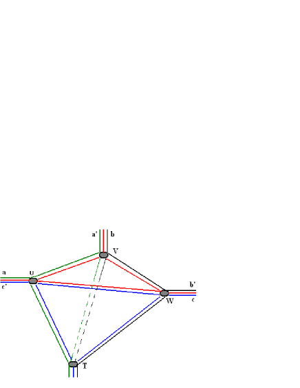
Figure 10: Toric web-diagram of the local elliptic curve using planar vertices in different planes. External and internal momenta have been expressed in terms of 2d partitions. 

Through this particular example, we would like to set up the basis of the non planar topological vertex formalism for the class of Calabi-Yau hypersurfaces associated with the supersymmetric gauged sigma model with non zero superpotential (2.7). More precisely, we consider the three following things:
(1) we derive the structure of the non planar 3- vertex C${}_{3}^{\left(np\right)}$. This vertex can be realized by the combination of at least two planar topological 3- vertices; say C${}_{3}^{\left(xy\right)}$ and C${}_{3}^{\left(yz\right)}$ living in the $xy$- and $yz$- planes respectively. Note that C${}_{3}^{\left(np\right)}$ has an interpretation in terms of 3d- partitions $\Pi,$ $\Lambda,$ $\Sigma,$ and $\Gamma$,

$$\mathcal{C}_{3}^{\left(np\right)}=\mathcal{C}_{\Pi\Lambda\Sigma\Gamma}.$$ (5.2)

(2) we give the explicit expression of the non planar topological 3-vertex C${}_{3}^{\left(np\right)}$; first in terms of products of the planar 3- vertices and then in terms of products of Schur functions $\mathcal{S}_{\xi}$.
(3) we calculate the explicit value of the topological partition function $\mathcal{Z}_{H_{3}}$ of the Calabi-Yau hypersurface $H_{3}^{\left(\infty\right)}$ by using C${}_{3}^{\left(np\right)}$.
With this programme in mind, we turn now to give details.

5.1 Deriving the non planar vertex C${}_{3}^{\left(np\right)}$

A direct way to get the structure of the non planar vertex C${}_{3}^{\left(np\right)}$ is to start from the web diagram of $H_{3}^{\left(\infty\right)}$ with the Calabi-Yau condition (4.17),

$$\sum_{i=0}^{4}q_{i}=3.$$ (5.3)

Then, use the remarkable relation between the toric graph of $H_{3}^{\left(\infty\right)}$ and the one corresponding to the normal bundle of the complex projective plane $NP^{2}$. The compact divisor $S_{2}$ of the hypersurface $H_{3}^{\left(\infty\right)}$ involves three intersecting complex projective planes $P_{1}^{2}$, $P_{2}^{2}$ and $P_{3}^{2}$; i.e

$$S_{2}=P_{1}^{2}\cup P_{2}^{2}\cup P_{3}^{2}$$ ,

(5.4)

with intersections as follows

$$P_{1}^{2}\cap P_{2}^{2}=\mathcal{C}_{3}$$ ,

,

,

(5.5)

where the curves $\mathcal{C}_{1}$, $\mathcal{C}_{2}$ and $\mathcal{C}_{3}$ are projective lines. This property implies that $H_{3}^{\left(\infty\right)}$ can be obtained by gluing three copies of $NP^{2}$ in a specific manner,

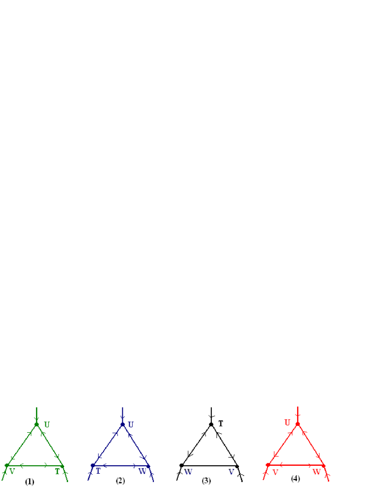
Figure 11: These are toric figures presenting the NP² ’s involved in making the CY hypersurface H${}_{3}^{\left(\infty\right)}$. The triangles $(1)$, $(2),$ $(3)$ and $(4)$ belong to different planes of the 3d- space. The arrows represent the incoming momenta. 

The various $NP^{2}$’s, represented by the web graphs of the figures (11), belong to different planes of the 3d- space and are associated with the triangles

$$UVT,\qquad UWT,\qquad VWT.$$ (5.6)

To get the hypersurface $H_{3}^{\left(\infty\right)}$ with $T^{2}\times R$ fibration, the triangle $UVW$ in figure (10) should be omitted because of the condition (5.3). Notice that like for figure (10), the web diagram of the hypersurface $H_{3}^{\left(\infty\right)}$ has four vertices denoted as $U$, $V$, $W$ and $T$ where the respective incoming momenta $\left\{\mathbf{u}_{i}\right\}$, $\left\{\mathbf{v}_{i}\right\}$, $\left\{\mathbf{w}_{i}\right\}$ and $\left\{\mathbf{t}_{i}\right\}$ add to zero,

$$\sum\limits_{i=1}^{4}\mathbf{u}_{i}=0$$ , , .

(5.7)

To get more insight on the vectors $\mathbf{u}_{i},$ $\mathbf{v}_{i}$, $\mathbf{w}_{i}$ and $\mathbf{t}_{i}$, let us give some details.

(i) Vertex $U$
The vector momenta $\mathbf{u}_{1}$, $\mathbf{u}_{2}$, $\mathbf{u}_{3}$ and $\mathbf{u}_{4}$, capturing the quantum numbers of the shrinking 1-cycles on the respective edges $E_{1}$, $E_{2}$, $E_{3}$ and $E_{4}$ ending on the vertex $U$, are given by the following 3- dimensional integer vectors

$$U:\left\{\begin{tabular}[]{lll}$\mathbf{u}_{1}$&$=$&$\left(-1,0,0\right)$\\ $\mathbf{u}_{2}$&$=$&$\left(-1,+1,0\right)$\\ $\mathbf{u}_{3}$&$=$&$\left(-1,0,+1\right)$\\ $\mathbf{u}_{4}$&$=$&$\left(+3,-1,-1\right)$\end{tabular}\right.$$ (5.8)

The Calabi-Yau condition at the vertex $U$ is given by the following conservation law,

$$\mathbf{u}_{1}\mathbf{+u}_{2}\mathbf{+u}_{3}\mathbf{+u}_{4}=\mathbf{0,}$$ (5.9)

in agreement with the property that all cycles shink to zero at the vertex. Notice also the two following features:
First, the condition (5.9) shows that only three of the four vectors $\mathbf{u}_{i}$ are linearly independent; they generate a 3d- vector space.
Second, the non planar vertex C${}_{3}^{\left(np\right)}$ is obtained by combining three planar vertices C${}_{3}^{\left(xy\right)}$, C${}_{3}^{\left(yz\right)}$ and C${}_{3}^{\left(zx\right)}$ which come from appropriate projections on 2d- vector spaces as follows,

$$U^{xy}:\left\{\begin{tabular}[]{l}$\mathbf{u}_{1}^{xy}=\left(-1,0,0\right)$\\ $\mathbf{u}_{2}^{xy}=\left(-1,1,0\right)$\\ $\mathbf{u}_{3}^{\prime xy}=\left(+2,-1,0\right)$\end{tabular}\right.$$, , ,

where the upper indices $\left(xy\right)$, $\left(yz\right)$, $\left(zx\right)$ stand for the $xy$- ,$yz$-, $zx$- planes respectively and where we have used the folding

$$\mathbf{u}_{3}^{\prime xy}=\mathbf{u}_{3}^{xy}+\mathbf{u}_{4}^{xy}$$ ,

.

(5.10)

The above 3- vertices $U^{xy}$, $U^{yz}$ and $U^{zx}$, respectively associated with the topological 3- vertices C${}_{3}^{\left(xy\right)}$, C${}_{3}^{\left(yz\right)}$ and C${}_{3}^{\left(zx\right)}$, obey the Calabi-Yau conditions

$$\mathbf{u}_{1}^{xy}+\mathbf{u}_{2}^{xy}+\mathbf{u}_{3}^{\prime xy}=\mathbf{0}$$ ,

,

.

(5.11)

As a result, the non planar topological vertex C${}_{3}^{\left(np\right)}$ is built from the 3- vertices C${}_{3}^{\left(xy\right)}$, C${}_{3}^{\left(yz\right)}$ and C${}_{3}^{\left(zx\right)}$ associated with the patches $U^{xy}$, $U^{yz}$ and $U^{zx}$. Notice that since $U^{xy}$, $U^{yz}$ and $U^{zx}$ belong to different planes, C${}_{3}^{\left(np\right)}$ is then a non planar vertex.

(ii) Vertex V
The incoming momenta $\left\{\mathbf{v}_{1},\mathbf{v}_{2},\mathbf{v}_{3},\mathbf{v}_{4}\right\}$ ending at the vertex $V$ of the web diagram of $H_{3}^{\left(\infty\right)}$ read as follows

$$V:\left\{\begin{tabular}[]{lll}$\mathbf{v}_{1}$&$=$&$\left(-1,-1,+3\right)$\\ $\mathbf{v}_{2}$&$=$&$\left(+1,0,-1\right)$\\ $\mathbf{v}_{3}$&$=$&$\left(0,+1,-1\right)$\\ $\mathbf{v}_{4}$&$=$&$\left(0,0,-1\right)$\end{tabular}\ \right..$$ (5.12)

The planar patches making the non planar topological vertex $V$ are given by,

$$V^{xy}:\left\{\begin{tabular}[]{l}$\mathbf{v}_{1}^{xy}=\left({\small-1,-1,0}\right)$\\ $\mathbf{v}_{2}^{xy}=\left({\small+1,0,0}\right)$\\ $\mathbf{v}_{3}^{xy}=\left({\small 0,+1,0}\right)$\end{tabular}\right.$$, , ,

They satisfy the conservation laws

$$\mathbf{v}_{1}^{xy}+\mathbf{v}_{2}^{xy}+\mathbf{v}_{3}^{xy}=\mathbf{0}$$ ,

,

,

(5.13)

encoding the properties that all cycles shrink at the vertex $V$.

(iii) Vertex W
Similarly, the incoming momenta $\left\{\mathbf{w}_{1},\mathbf{w}_{2},\mathbf{w}_{3},\mathbf{w}_{4}\right\}$ at the vertex $W$ read as follows,

$$W:\left\{\begin{array}[]{c}\mathbf{w}_{1}=\left({\small-1,3,-1}\right),\\ \mathbf{w}_{2}=\left(+{\small 1,-1,0}\right),\\ \mathbf{w}_{3}=\left({\small 0,-1,+1}\right),\\ \mathbf{w}_{4}=\left({\small 0,-1,0}\right).\end{array}\right.$$ (5.14)

We also have the following planar patches

$$W^{xy}:\left\{\begin{array}[]{c}\mathbf{w}_{1}^{\prime xy}\mathbf{=}\left(-1,2,0\right)\\ \mathbf{w}_{2}^{xy}\mathbf{=}\left(1,-1,0\right)\\ \mathbf{w}_{3}^{xy}\mathbf{=}\left(0,-1,0\right)\end{array}\right.$$, , ,

The momenta satisfy the Calabi-Yau conditions:

$$\mathbf{w}_{1}^{\prime xy}+\mathbf{w}_{2}^{xy}+\mathbf{w}_{3}^{xy}=\mathbf{0}$$ ,

,

.

(5.15)

(iv) Vertex T
This vertex, given by

$$T:\left\{\begin{tabular}[]{lll}$\mathbf{t}_{1}$&$=$&$\left(-1,-1,-1\right)$\\ $\mathbf{t}_{2}$&$=$&$\left(1,0,0\right)$\\ $\mathbf{t}_{3}$&$=$&$\left(0,1,0\right)$\\ $\mathbf{t}_{4}$&$=$&$\left(0,0,1\right)$\end{tabular}\ \right.,$$ (5.16)

is, in some sense a special vertex since it has a leg related to an external source with non zero momentum $\mathbf{t}_{1}$. The planar patches $T^{xy},$ $T^{yz}$ and $T^{zx}$ forming the non planar topological vertex $T$ are given by

$$T^{xy}:\left\{\begin{tabular}[]{l}$\mathbf{t}_{1}^{xy}=\left(-1,-1,0\right)$\\ $\mathbf{t}_{2}^{xy}=\left(1,0,0\right)$\\ $\mathbf{t}_{3}^{xy}=\left(0,1,0\right)$\end{tabular}\right.$$, , ,

with the Calabi-Yau conditions

$$\mathbf{t}_{1}^{xy}+\mathbf{t}_{2}^{xy}+\mathbf{t}_{3}^{xy}=\mathbf{0}$$ ,

,

.

(5.17)

Having derived the structure of the non planar vertex that is involved in the Calabi-Yau hypersurface $H_{3}^{\left(\infty\right)}$, we turn now to compute its expression in terms of the usual planar ones.

5.2 Non planar topological vertex C${}_{3}^{\left(np\right)}$

To get the explicit expression of the non planar topological vertex C${}_{3}^{\left(np\right)}$, we first focus on the vertex $U$. Then, we extend the obtained results to the other vertices $V$, $W$ and $T$.
A priori, a generic non planar vertex is made of at least two planar vertices belonging to different planes as shown in the figure (10). Based on this observation and motivated by the works [33, 31], we deduce that the expression of C${}_{3}^{\left(np\right)}$, associated with the vertex $U$, is given by the following relation

$$\mathcal{C}_{3}^{\left(np\right)}=\mathcal{C}_{3}^{\left(xy\right)}\times\mathcal{C}_{3}^{\left(zx\right)},$$ (5.18)

where the expression of C${}_{3}^{\left(xy\right)}$ and C${}_{3}^{\left(zx\right)}$ are topological 3-vertices as computed in [1]. To get the expression of C${}_{3}^{\left(np\right)}$ in terms of Schur functions, let us recall some useful results on the planar 3-vertex formalism.

Planar topological 3- vertex formalism
First recall that a toric Calabi-Yau threefold with a $T^{2}\times R$ special Lagrangian fibration has toric geometry represented by planar web diagrams. Following [1], the expression of the topological 3-vertex $\mathcal{C}_{\emptyset\emptyset\emptyset}$ without boundary conditions; i.e $\left(\lambda,\mu,\nu\right)=$ $\left(\emptyset,\emptyset,\emptyset\right)$, is given by

$$\mathcal{C}_{\emptyset\emptyset\emptyset}\left(q\right)=\mathop{\displaystyle\prod}\limits_{k=1}^{\infty}\left(\frac{1}{\left(1-q^{k}\right)^{k}}\right),$$ (5.19)

and describes the topological closed string amplitude on $C^{3}$ with $q=e^{-g_{s}}$ and $g_{s}$ being the closed string coupling constant. It happens that this relation is nothing but the 3d- MacMahon function $\mathcal{Z}_{3d}$ generating plane partitions.
Open strings ending on D- branes are implemented by introducing non trivial boundary conditions $\left(\lambda,\mu,\nu\right)$ on the edges of the 3-vertex. The topological 3- vertex associated with this configuration is denoted as $\mathcal{C}_{\lambda\mu\nu}(q)$ and its contribution reads, in terms of the Schur functions $\mathcal{S}_{\xi}\left(q\right)$, as follows

$$\mathcal{C}_{\lambda\mu\nu}(q)=q^{\kappa(\lambda)}\left[\mathcal{S}_{\nu^{T}}(q^{-\rho})\sum_{2d\text{ partitions }\eta}\mathcal{S}_{\lambda^{T}/\eta}(q^{-\nu-\rho})\mathcal{S}_{\mu/\eta}(q^{-\nu^{T}-\rho})\right].$$ (5.20)

where $\kappa(\lambda)=2\left(\left\|\lambda\right\|^{2}-\left|\lambda\right|\right)-2\left(\left\|\lambda^{T}\right\|^{2}-\left|\lambda^{T}\right|\right)$ is related to the Casimir of the representation of 2d partition $\lambda$, while $\nu^{T}$ represents the transpose of the Young diagram and $\mathcal{S}_{\lambda/\eta}(q)$ stands for the skew Schur function with $q^{-\nu-\rho}=\left(q^{-\nu_{1}-\frac{1}{2}},q^{-\nu_{2}-\frac{3}{2}},q^{-\nu_{3}-\frac{5}{2}}\ldots\right)$.

Determining C${}_{3}^{\left(np\right)}$
At $U$, the non planar topological vertex C${}_{3}^{\left(np\right)}$ (5.18) reads, by implementing the boundary conditions, as follows,

$$\mathcal{C}_{\mathrm{abcdef}}^{\left(np\right)}\left(q_{1},q_{2}\right)=\mathcal{C}_{\mathrm{ab}\text{{c}}}^{\left(xy\right)}\left(q_{1}\right)\times\delta_{\text{{c}}d}\times\mathcal{C}_{\mathrm{def}}^{\left(zx\right)}\left(q_{2}\right),$$ (5.21)

where $q_{1}$ and $q_{2}$ are two parameters which may be set as $q_{1}=q_{2}=e^{-g_{s}}$. The a, b, c, d, e, f stand for 2d- partitions encoding the configuration of D- branes which end on each edge of the toric diagram. The 3- vertex $\mathcal{C}_{\mathrm{abc}}^{\left(xy\right)}$ is a planar vertex in $xy$- plane while $\mathcal{C}_{\mathrm{def}}^{\left(zx\right)}$ is planar in the $zx$- plane. The factor $\delta_{\text{{c}}d}$ of eq(5.21) captures the data on the intersection between $\mathcal{C}_{\mathrm{abc}}^{\left(xy\right)}$ and $\mathcal{C}_{\mathrm{def}}^{\left(zx\right)}$. Using eq(5.20), we get

C$${}_{\mathrm{abcdef}}^{\left(np\right)}\left(q_{1},q_{2}\right)=$$

.

Similar relations are valid for the vertices $V$ and $W$; they read as follows,

C$${}_{\mathrm{a}^{\prime}\mathrm{b}^{\prime}\text{{c}}^{\prime}\text{d}^{\prime}\mathrm{e}^{\prime}\mathrm{f}^{\prime}}^{\left(np\right)}\left(V\right)$$ C ,

C C .

(5.22)

Regarding the patch $T$, the corresponding non planar topological vertex

$$\mathcal{C}_{\mathrm{\alpha\beta\gamma\delta\zeta\theta\lambda\mu\nu}}^{\left(np\right)}\left(T\right)$$

is made of three planar topological 3-vertices $\mathcal{C}_{\mathrm{\alpha\beta\gamma}}\left(T^{zx}\right)$, $\mathcal{C}_{\mathrm{\delta\zeta\theta}}\left(T^{yz}\right)$ and $\mathcal{C}_{\mathrm{\lambda\mu\nu}}\left(T^{zx}\right)$. We have

$$\mathcal{C}_{\mathrm{\alpha\beta\gamma\delta\zeta\theta\lambda\mu\nu}}^{\left(np\right)}\left(T\right)=\mathcal{C}_{\mathrm{\alpha\beta\gamma}}^{\left(xy\right)}\left(q_{1}\right)\times\delta_{\gamma\delta}\times\mathcal{C}_{\mathrm{\delta\zeta\theta}}^{\left(yz\right)}\left(q_{2}\right)\times\delta_{\mathrm{\theta\lambda}}\times\mathcal{C}_{\mathrm{\lambda\mu\nu}}^{\left(zx\right)}\left(q_{3}\right)\times\delta_{\beta\nu},$$ (5.23)

where $\mathcal{C}_{\mathrm{\alpha\beta\gamma}}^{\left(xy\right)}\left(q_{1}\right)$, $\mathcal{C}_{\mathrm{\delta\zeta\theta}}^{\left(yz\right)}\left(q_{2}\right)$ and $\mathcal{C}_{\mathrm{\lambda\mu\nu}}^{\left(zx\right)}\left(q_{3}\right)$ are as in eq(5.20).

5.3 Explicit expression of $\mathcal{Z}_{H_{3}}$

In this subsection, we derive the expression of $\mathcal{Z}_{H_{3}}$ by using the non planar topological vertex formalism. Starting from the diagram (10), which we put it in the form (12), we can determine $\mathcal{Z}_{H_{3}}$ by help of the cutting and gluing method of Aganagic et al.

Figure 12: Non planar graph representing elliptic curve as a toric manifold. Cutting the graph into four non planar 3-vertex.

Mimicking the planar topological vertex formalism and using eq(5.21-5.23), we obtain

$$\mathcal{Z}_{X_{3}}=\sum_{\left\{\varkappa\right\}}\left[\left(\mathcal{U}_{\omega\varphi^{\mathrm{T}}\rho\sigma^{\mathrm{T}}}\right)\left(\mathcal{V}_{\chi\rho^{\mathrm{T}}\psi\varsigma^{\mathrm{T}}}\right)\left(\mathcal{W}_{\iota\psi^{\mathrm{T}}\kappa\omega^{\mathrm{T}}}\right)\left(\mathcal{T}_{\varphi\kappa^{\mathrm{T}}\chi\sigma^{\mathrm{T}}\iota\varsigma^{\mathrm{T}}}\right)\mathcal{H}_{\omega\varphi\rho\sigma\chi\iota\kappa\psi\varsigma}\right]$$ (5.24)

where $\varkappa$ stands for the 2d- partitions $\omega,$ $\varphi,$ $\rho,$ $\sigma,$ $\chi,$ $\psi,$ $\varsigma,$ $\iota,$ $\kappa$ while $\mathcal{U}_{\omega\varphi^{\mathrm{T}}\rho\sigma^{\mathrm{T}}}$, $\mathcal{V}_{\chi\rho^{\mathrm{T}}\psi\varsigma^{\mathrm{T}}}$, $\mathcal{W}_{\iota\psi^{\mathrm{T}}\kappa\omega^{\mathrm{T}}}$, and $\mathcal{T}_{\varphi\kappa^{\mathrm{T}}\chi\sigma^{\mathrm{T}}\iota\varsigma^{\mathrm{T}}}$  represent the non planar vertex which read in terms of the planar topological 3-vertex $\mathcal{C}_{\alpha\beta\gamma}$ as follows

$$\mathcal{U}_{\omega\varphi^{\mathrm{T}}\rho\sigma^{\mathrm{T}}}$$ C ,

C ,

C ,

(5.25)

and

$$\mathcal{T}_{\sigma\chi^{\mathrm{T}}\iota^{\mathrm{T}}\varphi\kappa^{\mathrm{T}}\varsigma^{\mathrm{T}}}$$ C ,

.

(5.26)

The term $\mathcal{H}_{\omega\varphi\rho\sigma\chi\psi\varsigma\iota\kappa}=\prod\nolimits_{\varkappa=\omega,\varphi,\rho,\sigma,\chi,\psi,\varsigma,\iota,\kappa}(-e^{-t})^{\left|\varkappa\right|}q^{\kappa\left(\varkappa\right)}$ is the framing factor.

6 Conlusion

In this paper, we have studied the topological string theory on the special class of toric Calabi-Yau hypersurfaces which are realized in terms of supersymmetric gauged linear sigma model with non zero gauge invariant superpotential $\mathcal{W}\left(\Phi\right)\neq 0$.
Recall that for the case where there is no matter self- interaction ($\mathcal{W}\left(\Phi\right)=0$) the Calabi-Yau threefold is described by the equations of motion (2.4) of the auxiliary fields D^a in the gauge multiplets. In this case the topological 3- vertex is planar and the topological string amplitudes on this kind of toric Calabi-Yau threefolds with $T^{2}\times R$ fibration, is obtained by cutting and gluing method as done in [1].
In the case where $\mathcal{W}\left(\Phi\right)\neq 0$, one has moreover extra constraint eqs on the complex scalar field variables coming from the equations of motion of the auxiliary fields F in the chiral superfields. The resulting local Calabi-Yau threefolds are still toric; but the topological vertex is non planar.
In the present study we have made a step towards the developments of non planar topological vertex formalism by focusing on the example of the Calabi-Yau hypersurface $H_{3}$ with $R\times T^{2}$ fibration. We have derived the general structure of the non planar topological vertex C${}_{3}^{\left(np\right)}$ and its explicit expression as a product of the planar ones. We have also used this formalism to compute the partition function of $H_{3}$. From the analysis on the example of the local elliptic curve in large complex structure, we have learnt  that the non planar vertex shares features with the 4- vertex of CY4- folds and has an interpretation in terms of 3d- partitions. Further progress in this issues will be given in a future occasion.

Acknowledgement 1

This research work is supported by the program Protars III D12/25. BD and HJ would like to thank ICTP for kind hospitality where part of this work has been done.

7 Appendix

For solving the local Gromov-Witten theory of curves, several methods have been developed. One of them has been worked out by Bryan and Pandharipande in [31, 32] by using the localization and degeneration methods. The basic integrals in the local Gromov-Witten theory of $P^{1}$ are evaluated exactly by localization while the degeneration is required to capture higher genus curves. Amongst the interesting results gotten in [31, 32]; we quote the computation of the partition function of local Gromov-Witten invariants of curves in Calabi Yau threefolds. The degeneration method corresponds to splitting a genus $g$ surface $X$ along a separating non-singular divisor $B\subset X$ to obtain two surfaces $(X_{1},B)$ and $(X_{2},B)$ of genus $g_{1}$ and $g_{2}$.

$$Z(X)$$

(7.1)

It follows from this analysis that local Gromov-Witten theory of curves is closely related to q-deformed 2D Yang-Mills theory and bound states of BPS black holes obtained by the string theoretic method [8]. More explicitly; Vafa used the topological vertex method for a particular class of local threefolds involving the total space of a direct sum of a line bundle and its inverse on elliptic curve $T^{2}$. This study leads to the following partition function of $2d$ $U(N)$ Yang-Mills on $T^{2}$

$$Z^{YM}\sim Z_{+}^{YM}Z_{-}^{YM}=Z_{top}\bar{Z}_{top}$$

that appears as a product of a holomorphic and an anti-holomorphic partition function and where $Z_{top}$ is expressed as follows

$$Z_{top}=\sum\limits_{R}q^{mk(R)/2}exp(-t|R|).$$

Recall that $k(R)$ is the term of Casimir, $|R|$ the number of boxes of the Young diagram R, $exp(-t|R|)$ is the propagator and $q^{mk(R)/2}$.is the framing factor. This partition function coincides exactly with the one calculed in page 34 of [31].
In our present work, we have presented the main lines of the non-planar topological vertex formalism to solving the theory of local curves for the special class of toric Calabi-Yau hypersurfaces. The formalism used here for computing the expression of partition function of degenerate elliptic curve $g=1$ can also be extended to compute the partition function of degenerate higher genus elliptic curve. For the case $g=2$ for instance, the closed topological string partition function of the local $g$- Riemann surface in the large complex structures limit, we have

$$Z\left(q,Q\right)=\sum_{\xi_{1},\xi_{2}}\left(-Q\right)^{\left|\xi_{1}\right|+\left|\xi_{2}\right|}Z_{\xi_{1},\xi_{2}}^{\left(g=1\right)}(q)f_{\xi_{1},\xi_{2}}Z_{\xi_{1}^{T},\xi_{2}^{T}}^{\left(g=1\right)}$$

and is obtained by gluing two genus $g=1$ open string partition functions (5.24) together to form the closed string partition function.
Notice that the non planar topological vertex eq(5.24), deduced from the ramification of the non planar vertex as the union of two planar topological vertices $C^{1}\cup C^{2}$ in the two distinct plane $xy$ and $zx$ respectively eq(5.18), has a connection with the mathematical and stringy methods. presented previously. This link follows obviously from the identification of eq(5.18) with Bryan and Pandharipande formula (7.1).
From the above brief description; it follows that our non-planar topological vertex formalism should be though of as a different, but equivalent, way for solving the theory of local curves.

References

- [1] Mina Aganagic, Albrecht Klemm, Marcos Marino, Cumrun Vafa , The Topological Vertex,Commun. Math. Phys. 254 (2005) 425-478, hep-th/0305132.
- [2] Amer Iqbal, Can Kozcaz, Cumrun Vafa , The Refined Topological Vertex, hep-th/0701156.
- [3] Andrei Okounkov, Nikolai Reshetikhin, Cumrun Vafa, Quantum Calabi-Yau and Classical Crystals, arXiv:hep-th/0309208.
- [4] Sergei Gukov, Amer Iqbal, Can Kozcaz, Cumrun Vafa , Link Homologies and the Refined Topological Vertex, arXiv:0705.1368.
- [5] A. Iqbal, A-K Kashani-Poor, The Vertex on a Strip, hep-th/0410174.
- [6] M. Bershadsky, S. Cecotti, H. Ooguri and C. Vafa, “Kodaira-Spencer theory of gravity and exact results for quantum string amplitudes,” Commun. Math. Phys.165, 311 (1994), hep-th/9309140.
- [7] E. Witten, Chern-Simons Gauge Theory As A String Theory, Prog. Math. 133 (1995) 637 hep-th/9207094.
- [8] C. Vafa, Two dimensional Yang-Mills, black holes and topological strings, hep-th/0406058.
- [9] M. Aganagic, H. Ooguri, N. Saulina, C. Vafa, Black Holes, q-Deformed 2d Yang-Mills, and Non-perturbative Topological Strings, Nucl. Phys. B715 (2005) 304-348, hep-th/0411280.
- [10] R. Dijkgraaf, E. Verlinde, H. Verlinde, “Notes on topological string theory and twodimensional topological gravity in String theory and quantum gravity, World Scientific Publishing, p. 91, (1991)
-
[11]
E. H. Saidi, M. B. Sedra, Topological string in harmonic
space and correlation functions in S3 stringy cosmology, Nucl.
Phys. B748 (2006) 380-457, hep-th/0604204.
R. Ahl Laamara, L.B. Drissi, E.H. Saidi, D-string fluid in conifold: I &II. Nucl. Phys. B748 (2006) 380-457, hep-th/0604204, Nucl. Phys. B749 (2006) 206-224, hep-th/0605209.
E. H. Saidi, Topological SL(2) Gauge Theory on Conifold, hep-th/0601020. - [12] A. Neitzke and C. Vafa, “Topological Strings and their Physical Applications,” hep-th/0410178.
- [13] I. Antoniadis, S. Hohenegger, Topological Amplitudes and Physical Couplings in String Theory, arXiv:hep-th/0701290.
- [14] M. Aganagic, D. Jafferis, N. Saulina, Branes, Black Holes and Topological Strings on Toric Calabi-Yau Manifolds, hep-th/0512245.
- [15] Piotr Sulkowski, Crystal Model for the Closed Topological Vertex Geometry, JHEP 0612 (2006) 030, arXiv:hep-th/0606055.
- [16] Yukiko Konishi, Satoshi Minabe, Flop invariance of the topological vertex, arXiv:math/0601352,
- [17] Jun Li, Chiu-Chu Melissa Liu, Kefeng Liu, Jian Zhou, A Mathematical Theory of the Topological Vertex, arXiv:math/0408426.
- [18] Lalla Btissam Drissi, Houda Jehjouh, El Hassan Saidi, Non Planar Topological vertex Formalism, hep-th/0712.4249, Nuclear Physics B 804 (2008) 307–341.
- [19] Lalla Btissam Drissi, Houda Jehjouh, El Hassan Saidi, Generalized MacMahon G(q) as q-deformed CFT Correlation Function, arXiv:0801.2661, Nuclear Physics B 801 (2008) 316–345.
- [20] L.B Drissi, H. Jehjouh, E.H Saidi, Topological String on Local Elliptic Curve with Large Complex Structure, Afr Journal Of Mathematical Physics, Volume 6 (2008) 95-103.
- [21] N.C. Leung, C. Vafa, Branes and Toric Geometry, Adv. Theor. Math.Phys. 2 (1998) 91-118, hep-th/9711013.
- [22] Johanna Knapp, D-Branes in Topological String Theory, arXiv:0709.2045.
- [23] W. Fulton, Introduction to Toric Varieties, Annals of Math. Studies, No.131, Princeton University Press, 1993.
- [24] Dominic Joyce, Lectures on Calabi-Yau and special Lagrangian geometry, arXiv:math/0108088.
- [25] R. Ahl Laamara, A. Belhaj, L.B. Drissi, E.H. Saidi, On Local Calabi-Yau Supermanifolds and Their Mirrors, J.Phys. A39 (2006) 5965-5978, arXiv:hep-th/0601215.
- [26] Riccardo Ricci, Super Calabi-Yau’s and Special Lagrangians, JHEP 0703 (2007) 048, arXiv:hep-th/0511284.
- [27] Edward Witten, Phases of N=2 Theories In Two Dimensions, Nucl.Phys. B403 (1993) 159-222 arXiv:hep-th/9301042.
- [28] W. Lerche, C. Vafa and N. Warner, Nucl. Phys. B324 (1989) 427.
- [29] M. Ait Benhaddou, E. H Saidi, Explicit Analysis of Kahler Deformations in 4D N=1 Supersymmetric Quiver Theories, Phys. Lett. B575 (2003) 100-110, hep-th/0307103.
- [30] R. Ahl Laamara, M. Ait Ben Haddou, A Belhaj, L.B Drissi, E.H Saidi , RG Cascades in Hyperbolic Quiver Gauge Theories, Nucl.Phys. B702 (2004) 163-188, arXiv:hep-th/0405222.
- [31] J. Bryan and R. Pandharipande, The local Gromov-Witten theory of curves, arXiv:math/0411037.
- [32] J. Bryan, R. Pandharipande, Curves in Calabi-Yau 3-folds and Topological Quantum Field Theory, arXiv:math/0306316.
- [33] Dagan Karp, Chiu-Chu Melissa Liu, Andmarcos Marino, The local Gromov-Witten invariants of configurations of rational curves, arXiv:math/0506488v2.
- [34] Lalla Btissam Drissi, Houda Jehjouh, El Hassan Saidi, Refining the Shifted Topological Vertex, To appear in Journal of Mathematical Pysics, January issue (2009), American Institute of Physics, arXiv:0812.0513, [hep-th].