Tools for Charged Higgs Bosons

Abstract:

In order to identify the Higgs sector realized in nature, the predictions for Higgs boson masses, production cross sections and decay widths have to be compared with experimental results. We give a brief overview about computer codes for the evaluation of the properties of charged Higgs bosons, mostly focusing on the case of the Minimal Supersymmetric Standard Model (MSSM). We briefly review the relevance of the various contributions to the charged MSSM Higgs boson mass arising at the one-loop level.

1 Introdcution

Identifying the mechanism of electroweak symmetry breaking will be one of the main goals of the LHC. Many possibilities have been studied in the past, of which the most popular ones are the Higgs mechanism within the Standard Model (SM) [1], the Two Higgs Doublet Model (THDM) [2], and within supersymmetric (SUSY) models [3], which naturally contain at least two Higgs doublets. While the SM contains only one physical (neutral) Higgs boson, models with two Higgs doublets contain, besides three neutral Higgs bosons, at least two charged Higgs bosons, $H^{\pm}$. Any evidence for a charged Higgs boson would be an unambiguous sign of an extended Higgs sector, i.e. of physics beyond the SM.

In order to identify the Higgs sector realized in nature, the predictions for couplings to SM fermions and bosons as well as self-couplings have to be compared with the experimental results. To perform this task precise theory predictions are needed for Higgs production cross sections and decay widths (or at best for complete processes). Here we give a brief overview about this kind of codes concerning the charged Higgs bosons. A recent overview about codes and tools for SUSY can be found in Ref. [4].

Within the THDM the Higgs potential contains 14 independent parameters, and the mass of the charged Higgs boson, $M_{H^{\pm}}$, is usually treated as a free parameter. Consequently, no code exists predicting $M_{H^{\pm}}$. However, tree-level production cross sections and decay width can be evaluated with codes like MadGraph [5], Pythia [6], Sherpa [7] or Herwig [8]. We are not aware of codes containing higher-order corrections to charged Higgs boson processes. However, this could be done in principle with FeynArts/FormCalc [9, 10], for which the THDM model file is available.

Within SUSY many results for the charged Higgs boson beyond the tree-level are available in the Minimal Supersymmetric Standard Model (MSSM), see below. The only code that contains higher-order corrections for a charged Higgs boson beyond the MSSM is NMSSMTools [11], providing masses, production cross sections and decay widths in the NMSSM, i.e. the MSSM with an additional Higgs singlet. In the following we will focus on the MSSM.

2 The charged Higgs in the MSSM

The Higgs sector of the MSSM contains two Higgs doublets, leading to five physical Higgs bosons. At tree-level these are the light and heavy ${\cal CP}$-even $h$ and $H$, the ${\cal CP}$-odd $A$ and the charged $H^{\pm}$. At lowest order the Higgs sector can be described besides the SM parameters by two additional independent parameters, chosen to be the mass of the $A$ boson, $M_{A}$ (in the case of vanishing complex phases), and $\tan\beta\equiv v_{2}/v_{1}$, the ratio of the two vacuum expectation values. Accordingly, all other masses and couplings can be predicted at tree-level, e.g. the charged Higgs boson mass

$$m_{H^{\pm}}^{2}=M_{A}^{2}+M_{W}^{2}~{}.$$ (1)

$M_{Z,W}$ denote the masses of the $Z$ and $W$ boson, respectively. This tree-level relation receives higher-order corrections, where the loop corrected charged Higgs-boson mass is denoted as $M_{H^{\pm}}$.

The charged Higgs bosons of the MSSM (or a more general Two Higgs Doublet Model) have been searched at LEP and the Tevatron, and will be searched for at the LHC and the ILC. The LEP searches [12, 13], yielded a bound of $M_{H^{\pm}}\;\raisebox{-3.00003pt}{$\stackrel{{\scriptstyle\displaystyle>}}{{\sim}}$}\;80\,\,\mathrm{GeV}$ [14]. The Tevatron is especially sensitive at low $M_{A}$ and large $\tan\beta$, extending the LEP bounds in this region of parameter space [15]. Also at the LHC the prospects for charged Higgs boson searches are best at large $\tan\beta$, reaching up to $M_{A}\;\raisebox{-3.00003pt}{$\stackrel{{\scriptstyle\displaystyle<}}{{\sim}}$}\;800\,\,\mathrm{GeV}$ [16, 17, 18]. At the ILC, if the charged Higgs is in the kinematical reach, a high-precision determination of the charged Higgs boson properties will be possible [19, 20].

Many computer codes exists to evaluate various properties of the (charged) Higgs boson in the MSSM:

• RGE running from a high-energy scale to the electroweak (EW) scale for SUSY parameter is provided, for instance, by SoftSusy [21], Spheno [22], Suspect [23] or Isajet [24]. Subsequently they evaluate $M_{H^{\pm}}$ including (some) one-loop corrections.

• Three codes exist for the calculation of $M_{H^{\pm}}$ and the various decay widths, FeynHiggs [25, 26, 27, 28, 29], CPsuperH [30] and Hdecay [31]. More details on the evaluations can be found below.

• Calculations for the charged Higgs production at the LHC have been performed in
  Refs. [32, 33] (see also Ref. [34]), for the production in association with a $W$ boson in Ref. [35] and for the production of a $H^{\pm}H^{\mp}$ pair in Ref. [36]. However, no dedicated code exists. The calculation of Refs. [32, 33] has recently been implemented into Prospino [37] and is also included in FeynHiggs [25, 26, 27, 28, 29] (including the $\Delta_{b}$ corrections, see below). More details on recent higher-order corrections can be found in Ref. [38]. For the $H^{\pm}$ production at the ILC we are only aware of one code for the calculation of $e^{+}e^{-}\to W^{\pm}H^{\mp}$ [39].

• Event generators can produce events with a charged MSSM Higgs boson: Pythia [6], Sherpa [7] or Herwig [8]. They contain only relatively few corrections to the Higgs boson mass or decay widths. However, they can be linked to the dedicated spectrum and decay calculators via the SUSY Les Houches Accord [40].

• Indirect constraints on the mass and couplings of the charged MSSM Higgs boson can be set via (e.g.) $B$-physics observables. One dedicated code for this is SuperIso [41], another one is described in Ref. [42]. Other codes contain some $B$-physics observables as an additional check on the MSSM parameter space. Examples are MicrOMEGAs [43], CPsuperH [30] or FeynHiggs [25, 26, 27, 28, 29]. LEP and Tevatron bounds on the charged Higgs boson searches are currently implemented into HiggsBounds [44].

A “comparison” of the dedicated mass and decay width calculators has to be split up into the case of the MSSM with real parameters (rMSSM) and the MSSM with complex parameters (cMSSM). Hdecay is purely for real parameters. CPsuperH and FeynHiggs can handle also parameters with complex phases (for instance $A_{t}$, $A_{b}$, $M_{3}$, $\mu$, …). The following corrections to $M_{H^{\pm}}$ are implemented into the three codes (we do not go into details concerning the attempt to capture three-loop corrections):

• Hdecay: $M_{H^{\pm}}$ in the rMSSM:
  $M_{A}$ is input parameter, and the higher-order corrections to $M_{H^{\pm}}$ are evaluated. The calculation of Ref. [45] (including corrections up to the two-loop level) has been exteded to the complete Higgs potential and thus to $M_{H^{\pm}}$, including the $\Delta_{b}$ corrections.

• CPsuperH: $M_{H^{\pm}}$ in the cMSSM:
  $M_{H^{\pm}}$ is an input parameter, and the higher-order corrections appear as shifts to the neutral Higgs boson masses. A large set of one-loop corrections are supplemented by two-loop contributions obtained by RGE improvements, see Ref. [46] and references therein. The complex $\Delta_{b}$ corrections (see below) are included.

• FeynHiggs: $M_{H^{\pm}}$ in the rMSSM:
  $M_{A}$ is an input parameter, and the higher-order corrections to $M_{H^{\pm}}$ are evaluated. They comprise the full set of one-loop contributions [28] and various two-loop corrections as summarized in Ref. [27].
  FeynHiggs: $M_{H^{\pm}}$ in the cMSSM:
  $M_{H^{\pm}}$ is an input parameter, and the higher-order corrections appear as shifts to the neutral Higgs boson masses. The calculation comprises the full set of one-loop contributions [28] and the ${\cal O}(\alpha_{t}\alpha_{s})$ corrections as given in Ref. [29].

An overview about the various charged MSSM Higgs boson properties implemented into FeynHiggs, CPsuperH and Hdecay is shown in Tab. 1. The evaluation of the charged Higgs decay contains in all three codes the contribution coming from $\Delta_{b}$ (see below). However, the effect of complex phases in the various calculations is taken into account only in FeynHiggs and CPsuperH. The Higgs self-couplings are understood to contain an $H^{+}H^{-}$ pair. The LHC production cross section calculation in in FeynHiggs is based on Refs. [32, 33], supplemented by the $\Delta_{b}$ corrections. We also list ${\rm BR}(t\to H^{+}\bar{b})$, which be used to evaluate the charged Higgs production cross section for $M_{H^{\pm}}<m_{t}$ at the Tevatron or the LHC.

	FeynHiggs	CPsuperH	Hdecay
$\Gamma_{\rm tot}$	$\surd$	$\surd$	$\surd$
${\rm BR}(H^{+}\to f^{(*)}\bar{f}^{\prime})$	$\surd$	$\surd$	$\surd$
${\rm BR}(H^{+}\to h_{i}W^{(*)})$	$\surd$	$\surd$	$\surd$
${\rm BR}(H^{+}\to\tilde{f}_{i}\tilde{f}_{j}^{\prime})$	$\surd$	$\surd$	$\surd$
${\rm BR}(H^{+}\to\tilde{\chi}^{0}_{i}\tilde{\chi}^{+}_{j})$	$\surd$	$\surd$	$\surd$
Higgs triple self-couplings	$\surd$	$\surd$
Higgs quartic self-couplings		$\surd$
$\sigma(pp\to H^{+}+X)$ at the LHC	$\surd$
${\rm BR}(t\to H^{+}\bar{b})$	$\surd$	$\surd$

Table 1: Overview about the various charged MSSM Higgs boson properties implemented into FeynHiggs, CPsuperH and Hdecay. $f$ denotes a SM fermion, $h_{i}$ ($i=1,2,3$) are the three neutral Higgs bosons, $\tilde{f}_{i}$ denotes a scalar fermion, and $\tilde{\chi}^{0}_{i}$, $\tilde{\chi}^{\pm}_{k}$ are the neutralinos and charginos, respectively. The evaluation of the charged Higgs decay contains in all three codes the contribution coming from $\Delta_{b}$. The effect of complex phases in the various calculations is taken into account only in FeynHiggs and CPsuperH. Higgs self-couplings are understood to contain an $H^{+}H^{-}$ pair. The LHC production cross section calculation in in FeynHiggs is based on Refs. [32, 33], supplemented by the $\Delta_{b}$ corrections. The ${\rm BR}(t\to H^{+}\bar{b})$ can be used to evaluate the charged Higgs production cross section for $M_{H^{\pm}}<m_{t}$.

3 Relevance of higher-order corrections to $M_{H^{\pm}}$

3.1 The higher-order corrections

As mentioned above, the charged Higgs boson mass, see Eq. (1), receives higher-order corrections, which are (at different levels of sophistication) implemented into public codes. In a first step in Ref. [48] leading corrections to the sum rule given in Eq. (1) have been evaluated. Then one-loop corrections from $t/b$ and $\tilde{t}/\tilde{b}$ loops have been derived in Refs. [49, 50]. These were extended to the one-loop leading logarithmic terms from all sectors of the MSSM in Ref. [51]. The first full one-loop calculation in the Feynman-diagrammatic (FD) approach has been performed in Ref. [52], and re-evaluated more recently in Refs. [53, 28]. Within the FD approach the leading ${\cal O}(\alpha_{t}\alpha_{s})$ two-loop terms have recently been obtained in Ref. [29, 54]. In the following we will focus on the one-loop corrections.

Within the FD approach the charged Higgs boson pole mass, $M_{H^{\pm}}^{2}$, is obtained at the one-loop level by solving the equation

$$p^{2}-m_{H^{\pm}}^{2}+\hat{\Sigma}_{H^{+}H^{-}}^{(1)}(p^{2})=0~{}.$$ (2)

$\hat{\Sigma}_{H^{+}H^{-}}^{(1)}(p^{2})$ denotes the renormalized one-loop charged Higgs boson self-energy. Details about the calculation and the full one-loop evaluation can be found in Refs. [28, 53].

Another class of higher-order corrections that is formally of two-loop order is normally included already into the one-loop result. These corrections originate from the contributions to Higgs boson self-energies from the bottom/sbottom sector enhanced by $\mu\,\tan\beta$. Large higher-order effects can in particular occur in the relation between the bottom-quark mass and the bottom Yukawa coupling at large $\tan\beta$. Because the $\tan\beta$-enhanced contributions can be numerically relevant, an accurate determination of $h_{b}$ from the experimental value of the bottom mass requires a resummation of such effects to all orders in the perturbative expansion, as described in Refs. [55, 56]. Effectively the bottom Yukawa coupling is given by

$$\frac{g}{2M_{W}}\frac{\overline{m}_{b}}{1+\Delta_{b}}\quad~{}{\rm with}~{}\quad\overline{m}_{b}\;\equiv\;\overline{m}_{b}^{\overline{\mathrm{DR}}}(Q)\;=\;\overline{m}_{b}^{\overline{\mathrm{MS}}}(Q)\left(1+\frac{4\,\alpha_{s}}{3\,\pi}\right)~{}.$$ (3)

$\overline{m}_{b}$ denotes the running $\overline{\mathrm{DR}}$ bottom quark mass at the mass scale $Q$, where $\overline{m}_{b}^{\overline{\mathrm{MS}}}$ includes the SM QCD corrections. The leading one-loop contribution $\Delta_{b}$ in the limit of $M_{\rm SUSY}\gg m_{t}$ and $\tan\beta\gg 1$ takes the simple form [57]

$$\Delta_{b} =\frac{2\alpha_{s}}{3\,\pi}\,M_{3}^{*}\,\mu^{*}\,\tan\beta\,\times\,I(m_{\tilde{b}_{1}},m_{\tilde{b}_{2}},|M_{3}|)+\frac{\alpha_{t}}{4\,\pi}\,A_{t}^{*}\,\mu^{*}\,\tan\beta\,\times\,I(m_{\tilde{t}_{1}},m_{\tilde{t}_{2}},|\mu|)~{},$$ (4)

where the function $I$ arises from the one-loop vertex diagram and scales as
$I(a,b,c)\sim 1/\mbox{max}(a^{2},b^{2},c^{2})$. Here $m_{\tilde{t}_{1}},m_{\tilde{t}_{2}}$ and $m_{\tilde{b}_{1}},m_{\tilde{b}_{2}}$ denote the two scalar top and bottom masses, respectively. $|M_{3}|$ is the gluino mass parameter, $\mu$ is the Higgs mixing parameter, and $A_{t}$ denotes the trilinear Higgs-stop coupling. This type of higher-order corrections being formally beyond the one-loop level are included into the Yukawa couplings appearing in the one-loop result.

3.2 Numerical analysis

The higher-order corrected Higgs-boson sector has been evaluated with the help of the Fortran code FeynHiggs [26, 25, 27, 28]. The goal for the theory precision in $M_{H^{\pm}}$ should be the anticipated experimental resolution or better, where an accuracy of $\sim 1.5\,\,\mathrm{GeV}$ at the LHC and $\sim 0.5\,\,\mathrm{GeV}$ at the ILC could be achievable (see Ref. [54] for a more detailed discussion).

In Fig. 1 we show $\Delta M_{H^{\pm}}:=M_{H^{\pm}}-m_{H^{\pm}}$ with $M_{H^{\pm}}$ evaluated at the one-loop level in various steps of approximation. The results are obtained in the no-mixing scenario [58, 17]. The upper plot in Fig. 1 shows $\Delta M_{H^{\pm}}$ as a function of $\tan\beta$, while the lower plots depicts the variation with $\mu$. Both parameters enter the definition of $\Delta_{b}$ and are thus potentially important for a precise $M_{H^{\pm}}$ prediction. In both plots the solid lines represent the full one-loop result including the $\Delta_{b}$ resummation, see Eq. (4). The first approximation to this is shown as short-dashed line, where only the contributions from SM fermions and their SUSY partners (i.e. all squarks and sleptons) are taken into account, still including the $\Delta_{b}$ corrections. The next step of approximation is shown as dot-dashed lines, where only corrections from the $t/b$ and $\tilde{t}/\tilde{b}$ sector are included, still with the $\Delta_{b}$ resummation. The penultimate step of the approximation is to leave out the $\Delta_{b}$ corrections, but using $\overline{m}_{b}$ (i.e. including the SM QCD corrections, see Eq. (3)) in the Higgs boson couplings, shown as the long-dashed lines. The final step in the approximation is to drop the SM QCD corrections, i.e. replacing $\overline{m}_{b}$ by $m_{b}$ in the Higgs Yukawa couplings, shown as the dotted lines.

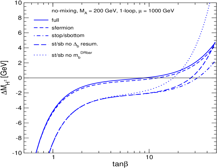
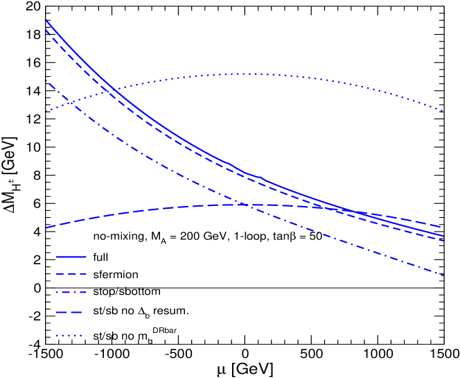
Figure 1: $\Delta M_{H^{\pm}}:=M_{H^{\pm}}-m_{H^{\pm}}$ is shown as a function of $M_{A}$ (upper plot), $\tan\beta$ (middle) and $\mu$ (lower) in the $m_{h}^{\rm max}$ scenario. $M_{H^{\pm}}$ is evaluated at the two-loop (solid) and the one-loop level (dashed).

The dependence on $\tan\beta$ is analyzed in the upper plot of Fig. 1 We show $\Delta M_{H^{\pm}}$ for $M_{A}=200\,\,\mathrm{GeV}$ and $\mu=1000\,\,\mathrm{GeV}$. The sign and size of the one-loop correction to $M_{H^{\pm}}$ depends strongly on $\tan\beta$, which appears the Higgs couplings to (s)fermions as well as in the $\Delta_{b}$ corrections. Negative corrections are reached for $\tan\beta\;\raisebox{-3.00003pt}{$\stackrel{{\scriptstyle\displaystyle<}}{{\sim}}$}\;10$ with $\Delta M_{H^{\pm}}\approx-10\,\,\mathrm{GeV}$ for $\tan\beta\approx 0.6$. It should be kept in mind that within the no-mixing scenario values of $\tan\beta$ around 1 are excluded by LEP Higgs searches [59, 60]. Positive values of $\Delta M_{H^{\pm}}$ are obtained for large $\tan\beta$ values, reaching $\Delta M_{H^{\pm}}\approx 2-6\,\,\mathrm{GeV}$ for $\tan\beta=50$. The effect of the non-sfermion sector (short-dashed lines) is small and stays below $0.5\,\,\mathrm{GeV}$. The Yukawa coupling independent effects (dot-dashed lines) are $\sim 2\,\,\mathrm{GeV}$, largely independent of $\tan\beta$. The contribution from the $\Delta_{b}$ effects is negligible for $\tan\beta\;\raisebox{-3.00003pt}{$\stackrel{{\scriptstyle\displaystyle<}}{{\sim}}$}\;5$ and grows with increasing $\tan\beta$, reaching values of up to $2\,\,\mathrm{GeV}$ for $\tan\beta=50$. For small values of $\mu$ (not shown here) these corrections stay very small even for the largest $\tan\beta$ values. The biggest effects on $M_{H^{\pm}}$ can arise from the inclusion of the SM QCD corrections to $m_{b}$ for $\tan\beta\;\raisebox{-3.00003pt}{$\stackrel{{\scriptstyle\displaystyle>}}{{\sim}}$}\;5$, reaching up to 5–$10\,\,\mathrm{GeV}$.

In order to analyze the dependence of the $M_{H^{\pm}}$ prediction on $\mu$ we show in lower plot of Fig. 1. $\Delta M_{H^{\pm}}$ as a function of $\mu$ for $M_{A}=200\,\,\mathrm{GeV}$ and $\tan\beta=50$. The pure $t/b/\tilde{t}/\tilde{b}$ corrections (dotted line) reach 12–$15\,\,\mathrm{GeV}$. Including the SM QCD corrections (long-dashed) strongly reduced the effect to the level of 4–$6\,\,\mathrm{GeV}$. In the next step the $\Delta_{b}$ effects are included (dot-dashed line). Due to $\Delta_{b}\propto\mu\,\tan\beta$ the inclusion of $\Delta_{b}$ results in a strong asymmetry of $M_{H^{\pm}}$ with a large correction for negative $\mu$ (corresponding to an enhanced bottom Yukawa coupling) and a much smaller correction for positive $\mu$ (corresponding to a suppressed bottom Yukawa coupling). $\Delta M_{H^{\pm}}$ now ranges from $\sim 14\,\,\mathrm{GeV}$ for $\mu=-1500\,\,\mathrm{GeV}$ to $\sim 1\,\,\mathrm{GeV}$ for $\mu=+1500\,\,\mathrm{GeV}$. Adding the corrections from the other (s)fermions yields an nearly $\mu$-independent upward shift of $\sim 2\,\,\mathrm{GeV}$. Including the non-(s)fermionic corrections result in another small upward shift of $\sim 0.5\,\,\mathrm{GeV}$. the overall one-loop effect ranges from $\Delta M_{H^{\pm}}\approx 19\,\,\mathrm{GeV}$ for $\mu=-1500\,\,\mathrm{GeV}$ down to $\Delta M_{H^{\pm}}\approx 3.5\,\,\mathrm{GeV}$ for $\mu=+1500\,\,\mathrm{GeV}$.

The results shown in Fig. 1 clearly indicate that for a precise $M_{H^{\pm}}$ prediction all contributions at the one-loop level have to be taken into account. Effects at the GeV level may be probed at the LHC and the ILC, see above. Thus, all parts of the one-loop calculation are relevant and should be taken into account in a precision analysis of the charged MSSM Higgs boson.

4 Summary

In order to identify the Higgs sector realized in nature, the predictions for Higgs boson masses, production cross sections and decay widths have to be compared with experimental results. We presented a brief overview about computer codes for the evaluation of the properties of charged Higgs bosons. While only few codes exist for the THDM or the NMSSM, many different tools are available for the MSSM. These comprise tools for RGE running, the evaluation of the charged Higgs boson mass, production cross sections and decay widths as well as event generators. Several codes provide indirect constraints on the charged Higgs boson sector via the evaluation of $B$-physics observables that can be checked against existing experimental data. We briefly compared the three codes available for the evaluation of the mass and decay properties of the charged MSSM Higgs, boson: FeynHiggs, CPsuperH and Hdecay. Finally, we briefly reviewed the relevance of the various contributions to the charged MSSM Higgs boson mass arising at the one-loop level. It was shown all parts of the one-loop calculation are relevant and should be taken into account in any precision analysis involving $M_{H^{\pm}}$.

Acknowledgements

We thank the organizers of cH${}^{\mbox{}^{\pm}}$arged 2008 for the invitation and the stimulating atmosphere.

References

- [1] S. Glashow, Nucl. Phys. 22 (1961) 579; S. Weinberg, Phys. Rev. Lett. 19 (1967) 19; A. Salam, in: Proceedings of the 8th Nobel Symposium, Editor N. Svartholm, Stockholm, 1968.
- [2] S. Weinberg, Phys. Rev. Lett. 37 (1976) 657; J. Gunion, H. Haber, G. Kane and S. Dawson, The Higgs Hunter’s Guide (Perseus Publishing, Cambridge, MA, 1990), and references therein.
- [3] H. Nilles, Phys. Rept. 110 (1984) 1; H. Haber and G. Kane, Phys. Rept. 117 (1985) 75; R. Barbieri, Riv. Nuovo Cim. 11 (1988) 1.
- [4] B. Allanach, arXiv:0805.2088 [hep-ph].
- [5] W. Long and T. Stelzer, Comput. Phys. Commun. 81 (1994) 357; F. Maltoni and T. Stelzer, JHEP 0302 (2003) 027.
- [6] T. Sjostrand et al., Comput. Phys. Commun. 135 (2001) 238.
- [7] T. Gleisberg et al., JHEP 0402 (2004) 056.
- [8] G. Corcella et al., arXiv:hep-ph/0210213; S. Moretti, K. Odagiri, P. Richardson, M. Seymour and B. Webber, JHEP 0204 (2002) 028.
- [9] J. Küblbeck, M. Böhm and A. Denner, Comput. Phys. Commun. 60 (1990) 165; T. Hahn, Comput. Phys. Commun. 140 (2001) 418; The program and the user’s guide are available via www.feynarts.de .
- [10] T. Hahn and M. Pérez-Victoria, Comput. Phys. Commun. 118 (1999) 153.
- [11] U. Ellwanger and C. Hugonie, Comput. Phys. Commun. 177 (2007) 399; Comput. Phys. Commun. 175 (2006) 290; U. Ellwanger, J. Gunion and C. Hugonie, JHEP 0502 (2005) 066.
- [12] A. Heister et al. [ALEPH Collaboration], Phys. Lett. B 543 (2002) 1. J. Abdallah et al. [DELPHI Collaboration], Eur. Phys. J. C 34 (2004) 399. P. Achard et al. [L3 Collaboration], Phys. Lett. B 575 (2003) 208. D. Horvath [OPAL Collaboration], Nucl. Phys. A 721 (2003) 453.
- [13] [LEP Higgs working group], arXiv:hep-ex/0107031.
-
[14]
P. Lutz et al. [LEP Higgs working group],
in preparation, see also:
ilcagenda.linearcollider.org/
contributionDisplay.py?contribId=153&sessionId=71&confId=1296 . - [15] [CDF Collaboration], Phys. Rev. Lett. 96 (2006) 042003; R. Eusebi, PhD thesis: “Search for charged Higgs in decay products from proton-antiproton collisions at ”, University of Rochester, 2005.
- [16] ATLAS Collaboration, Detector and Physics Performance Technical Design Report, CERN/LHCC/99-15 (1999); CMS Collaboration, Physics Technical Design Report, Volume 2. CERN/LHCC 2006-021.
- [17] M. Carena, S. Heinemeyer, C. Wagner and G. Weiglein, Eur. Phys. J. C 45 (2006) 797.
- [18] M. Hashemi, S. Heinemeyer, R. Kinnunen, A. Nikitenko and G. Weiglein, arXiv:0804.1228 [hep-ph]; S. Heinemeyer, A. Nikitenko and G. Weiglein, arXiv:0812.0524 [hep-ph];
- [19] S. Heinemeyer et al., arXiv:hep-ph/0511332.
- [20] A. Ferrari, talk given at the Carged 2006, Uppsala, Sweden, September 2006.
- [21] B. Allanach, Comput. Phys. Commun. 143 (2002) 305.
- [22] W. Porod, Comput. Phys. Commun. 153 (2003) 275.
- [23] A. Djouadi, J. Kneur and G. Moultaka, Comput. Phys. Commun. 176 (2007) 426.
- [24] F. Paige, S. Protopopescu, H. Baer and X. Tata, arXiv:hep-ph/0312045.
- [25] S. Heinemeyer, W. Hollik and G. Weiglein, Comput. Phys. Commun. 124 (2000) 76, see: www.feynhiggs.de .
- [26] S. Heinemeyer, W. Hollik and G. Weiglein, Eur. Phys. J. C 9 (1999) 343.
- [27] G. Degrassi, S. Heinemeyer, W. Hollik, P. Slavich and G. Weiglein, Eur. Phys. J. C 28 (2003) 133.
- [28] M. Frank, T. Hahn, S. Heinemeyer, W. Hollik, H. Rzehak and G. Weiglein, JHEP 0702 (2007) 047.
- [29] S. Heinemeyer, W. Hollik, H. Rzehak and G. Weiglein, Phys. Lett. B 652 (2007) 300.
- [30] J. Lee, A. Pilaftsis et al., Comput. Phys. Commun. 156 (2004) 283; J. Lee, M. Carena, J. Ellis, A. Pilaftsis and C. Wagner, arXiv:0712.2360 [hep-ph].
- [31] A. Djouadi, J. Kalinowski and M. Spira, Comput. Phys. Commun. 108 (1998) 56.
- [32] T. Plehn, Phys. Rev. D 67 (2003) 014018.
- [33] E. Berger, T. Han, J. Jiang and T. Plehn, Phys. Rev. D 71 (2005) 115012.
-
[34]
M. Krämer,
talk given at MSSM Higgs Physics at the LHC –
Theory meets Experiment, Santander, Spain, October 2008,
see: indico.ifca.es/indico/
contributionDisplay.py?contribId=8&sessionId=5&confId=175 . - [35] O. Brein, W. Hollik and S. Kanemura, Phys. Rev. D 63 (2001) 095001.
- [36] O. Brein and W. Hollik, Eur. Phys. J. C 13 (2000) 175.
- [37] T. Plehn, http://www.ph.ed.ac.uk/tplehn/prospino/ .
- [38] N. Kidonakis, arXiv:0811.4757 [hep-ph].
- [39] O. Brein and T. Hahn, Eur. Phys. J. 52 (2007) 397.
- [40] P. Skands et al., JHEP 0407 (2004) 036; B. Allanach et al., arXiv:0801.0045 [hep-ph].
- [41] F. Mahmoudi, Comput. Phys. Commun. 178 (2008) 745; arXiv:0808.3144 [hep-ph].
- [42] G. Isidori and P. Paradisi, Phys. Lett. B 639 (2006) 499; G. Isidori, F. Mescia, P. Paradisi and D. Temes, Phys. Rev. D 75 (2007) 115019.
- [43] G. Belanger, F. Boudjema, A. Pukhov and A. Semenov, Comput. Phys. Commun. 149 (2002) 103; Comput. Phys. Commun. 174 (2006) 577; Comput. Phys. Commun. 176 (2007) 367.
-
[44]
P. Bechtle, O. Brein, S. Heinemeyer, G. Weiglein
and K. Williams,
arXiv:0811.4169 [hep-ph], see:
www.ippp.dur.ac.uk/HiggsBounds . - [45] M. Carena, M. Quiros and C. Wagner, Nucl. Phys. B 461 (1996) 407.
- [46] A. Pilaftsis and C. Wagner, Nucl. Phys. B 553 (1999) 3; M. Carena, J. Ellis, A. Pilaftsis and C. Wagner, Nucl. Phys. B 586 (2000) 92.
- [47] M. Spira, private communication.
- [48] J. Gunion and A. Turski, Phys. Rev. D 39 (1989) 2701; Phys. Rev. D 40 (1989) 2333.
- [49] A. Brignole, J. Ellis, G. Ridolfi and F. Zwirner, Phys. Lett. B 271 (1991) 123.
- [50] A. Brignole, Phys. Lett. B 277 (1992) 313.
-
[51]
M. Diaz and H. Haber,
Phys. Rev. D 45 (1992) 4246;
M. Diaz, PhD thesis: “Radiative Corrections to Higgs Masses in the MSSM”, University of California, Santa Cruz, 1992, SCIPP–92/13. - [52] P. Chankowski, S. Pokorski and J. Rosiek, Phys. Lett. 274 (1992) 191.
- [53] M. Frank, PhD thesis: “Radiative Corrections in the Higgs Sector of the MSSM with Violation”, University of Karlsruhe, 2002, ISBN 3-937231-01-3.
- [54] M. Frank, T. Hahn, S. Heinemeyer, W. Hollik, H. Rzehak and G. Weiglein, MPP–2008–67.
- [55] M. Carena, D. Garcia, U. Nierste and C. Wagner, Nucl. Phys. B 577 (2000) 577.
- [56] H. Eberl, K. Hidaka, S. Kraml, W. Majerotto and Y. Yamada, Phys. Rev. D 62 (2000) 055006.
- [57] R. Hempfling, Phys. Rev. D 49 (1994) 6168; L. Hall, R. Rattazzi and U. Sarid, Phys. Rev. D 50 (1994) 7048; M. Carena, M. Olechowski, S. Pokorski and C. Wagner, Nucl. Phys. B 426 (1994) 269.
- [58] M. Carena, S. Heinemeyer, C. Wagner and G. Weiglein, Eur. Phys. J. C 26 (2003) 601.
- [59] [LEP Higgs working group], Phys. Lett. B 565 (2003) 61.
- [60] [LEP Higgs working group], Eur. Phys. J. C 47 (2006) 547.