Lab/UFR-HEP0803/GNPHE/0803/VACBT/0803
Refining the Shifted Topological Vertex

Abstract

We study aspects of the refining and shifting properties of the 3d MacMahon function $\mathcal{C}_{3}\left(q\right)$ used in topological string theory and BKP hierarchy. We derive the explicit expressions of the shifted topological vertex $\mathcal{S}_{\lambda\mu\nu}\left(q\right)$ and its refined version $\mathcal{T}_{\lambda\mu\nu}\left(q,t\right)$. These vertices complete results in literature.

Key words: 3d-Mac Mahon and generalizations, topological vertices, Young diagrams and plane partitions, Instantons, BKP hierarchy.

1 Introduction

In the last few years, there has been some interest in the study of the topological vertex formalism of toric Calabi-Yau threefold (CY3) [1]. This interest has followed the basic result according to which the topological vertex $\mathcal{C}_{\lambda\mu\nu}$ is a powerful tool to compute toric CY3 topological string amplitudes [1, 2, 3, 4]. It also came from the remarkable relation between $\mathcal{C}_{\lambda\mu\nu}$ and the Gromov-Witten invariants of genus g- curves in toric Calabi-Yau threefolds [5, 6, 7].
Recently it has been shown that the standard topological 3- vertex $\mathcal{C}_{\lambda\mu\nu}\left(q\right)$ may have two kinds of generalizations; one known as the refining of $\mathcal{C}_{\lambda\mu\nu}\left(q\right)$; and the other as its shifting.
In the first case, the refined topological vertex $\mathcal{R}_{\lambda\mu\nu}\left(q,t\right)$ is a two parameters function computing the refined topological string amplitudes of toric CY3s [8, 9, 18]. It has been found also that $\mathcal{R}_{\lambda\mu\nu}\left(q,t\right)$ computes as well  the Nekrasov’s instantons of the topological string free energy $F\left(X^{I},\varepsilon_{1},\varepsilon_{2}\right)$ of four dimensional $SU\left(N\right)$ gauge theories [10, 11]. In Nekrasov’s extension, the usual topological string coupling constant $g_{top}=\ln\left(\frac{1}{q}\right)$ gets replaced by the pair of parameters $\varepsilon_{1}$, $\varepsilon_{2}$ [12].
In the second case, the standard MacMahon function $\mathcal{C}_{3}\left(q\right)$ [3, 13] has been extended to the so called shifted partition function $\mathcal{S}_{3}\left(q\right)$. This is the generating function of the shifted plane partitions and it is used in the study of BKP hierarchy [14, 15, 16, 19].

The aim of this paper is to contribute to this matter by combining both the refining and the shifting operations to get the refined-shifted topological vertex $\mathcal{T}_{\lambda\mu\nu}\left(q,t\right)$ extending $\mathcal{R}_{\lambda\mu\nu}\left(q,t\right)$ and $\mathcal{S}_{3}\left(q\right)$ obtained recently in literature. More precisely, we want to complete the missing relations presented in the two following tables:
(i) First, we determine the refined version of the shifted MacMahon function $\mathcal{S}_{3}\left(q\right)$ obtained by Foda and Wheeler. The refined version of $\mathcal{S}_{3}\left(q\right)$, denoted below as $\mathcal{T}_{3}\left(q,t\right)$, is missing. It is a two parameters function generating shifted 3d- partitions needed to complete the table,

$$\qquad\mathcal{C}_{3}\left(q\right)=\emph{known:}$$  eq(2.4) eq(2.8)

shifting shifting

 eq(2.9)

(1.1)

(ii) Second, we extend the generalized MacMahon functions $\mathcal{S}_{3}\left(q\right)$ and $\mathcal{T}_{3}\left(q,t\right)$ by implementing boundary conditions captured by the strict 2d partitions $\widehat{\lambda},$ $\widehat{\mu}$ and $\widehat{\nu}$. The resulting $\mathcal{S}_{\widehat{\lambda}\widehat{\mu}\widehat{\nu}}\left(q\right)$ and $\mathcal{T}_{\widehat{\lambda}\widehat{\mu}\widehat{\nu}}\left(q,t\right)$ are also needed to complete the following table,

$$\qquad\mathcal{C}_{\lambda\mu\nu}\left(q\right)=\emph{known}$$   eq(2.1)  eq(2.6)

shifting   shifting

(1.2)

The organization of this paper is as follows: In section 2, we give generalities on topological vertices. In particular, we review briefly the expression of the constructions of the standard topological vertex $\mathcal{C}_{\lambda\mu\nu}\left(q\right)$, the refined one $\mathcal{R}_{\lambda\mu\nu}\left(q,t\right)$ and the shifted MacMahon function $\mathcal{S}_{3}\left(q\right)$. In section 3, we derive the explicit expression of the shifted topological vertex $\mathcal{S}_{\widehat{\lambda}\widehat{\mu}\widehat{\nu}}\left(q\right)$ of eq(1.2). In section 4, we compute the its refined version $\mathcal{T}_{\widehat{\lambda}\widehat{\mu}\widehat{\nu}}\left(q,t\right)$. In section 5, we give a conclusion and in section 6, we collect some useful tools as an appendix.

2 Topological vertex: a review

In this section, we review briefly some basic tools; in particular the explicit expressions of the three following topological vertices:
(1) the standard topological vertex denoted as $\mathcal{C}_{\lambda\mu\nu}\left(q\right)$.
(2) the refined topological vertex$\ \mathcal{R}_{\lambda\mu\nu}\left(q,t\right)$. This is a two parameters generalization of $\mathcal{C}_{\lambda\mu\nu}\left(q\right)$.
(3) the standard 3d- MacMahon function$\ \mathcal{C}_{3}\left(q\right)$, its refined version $\mathcal{R}_{3}\left(q,t\right)$ as well as the shifted 3d- MacMahon function $\mathcal{S}_{3}\left(q\right)$ obtained in [14].

These objects have interpretations in: (a) the topological string A- model in which $q=e^{-g_{s}}$ with $g_{s}$ being the topological string coupling constant. (b) the statistical mechanical models in which the parameter $q$ describes the Boltzmann weight $q=e^{-\frac{1}{KT}}$ with $T$ being absolute temperature [17, 13].

(a) Vertex $\mathcal{C}_{\lambda\mu\nu}\left(q\right)$
Following [3], the standard topological vertex $\mathcal{C}_{\lambda\mu\nu}\left(q\right)$, with boundary conditions in the $\left(x_{i},x_{j}\right)$ orthogonal planes of $\mathbb{Z}^{3}$ lattice given by the 2d partitions $\left(\lambda,\mu,\nu\right)$, can be defined in the transfer matrix method as follows:

$$\mathcal{C}_{\lambda\mu\nu}(q)=\mathrm{f}_{\lambda\mu\nu}\left\langle\nu^{t}\right|\left(\prod\limits_{t=0}^{\infty}q^{L_{0}}\Gamma_{+}(q^{-\lambda})\right)q^{L_{0}}\left(\prod\limits_{t=-\infty}^{-1}\Gamma_{-}(q^{-\lambda^{t}})q^{L_{0}}\right)\left|\mu\right\rangle,$$ (2.1)

where $\left|\xi\right\rangle$ is a generic 2d partition state ( a Young diagram), $\xi^{t}$ its transpose and $\left\langle\xi\right|L_{0}\left|\xi\right\rangle=\left|\xi\right|$ with $\left|\xi\right|$ being the number of boxes of the Young diagram. The operators $\Gamma_{\pm}\left(x\right)$ are vertex operators of the $c=1$ bosonic CFT₂, whose explicit expressions can be found in [13], and $\mathrm{f}_{\lambda\mu\nu}$ is a real number given by

$$\mathrm{f}_{\lambda\mu\nu}=\frac{q^{\frac{1}{2}(\left\|\lambda\right\|^{2}+\left\|\mu\right\|^{2}+\left\|\nu\right\|^{2})}}{q^{n(\nu)+n(\mu)}}\left(\prod\limits_{n=0}^{\infty}\left(1-q^{n}\right)^{n}\right).$$ (2.2)

For the particular case where there is no boundary condition, i.e $\lambda=\mu=\nu=\emptyset$, the vertex $\mathcal{C}_{\emptyset\emptyset\emptyset}\left(q\right)$ coincides exactly with the $3d$- MacMahon function $\mathcal{C}_{3}$:

$$\mathcal{C}_{3}\left(q\right)=\left\langle\emptyset\right|\left(\prod\limits_{t=0}^{\infty}q^{L_{0}}\Gamma_{+}(1)\right)q^{L_{0}}\left(\prod\limits_{t=-\infty}^{-1}\Gamma_{-}(1)q^{L_{0}}\right)\left|\emptyset\right\rangle.$$ (2.3)

The function $\mathcal{C}_{3}$, which reads explicitly as; see also eq(1.1),

$$\mathcal{C}_{3}\left(q\right)=\prod_{n=1}^{\infty}\left(\frac{1}{1-q^{n}}\right)^{n},$$ (2.4)

has several interpretations. It is the amplitude of the A-model topological closed string on $\mathbb{C}^{3};$ i.e $\mathcal{C}_{3}=\mathcal{C}_{\emptyset\emptyset\emptyset}$. It is also the generating function of 3d partitions,

$$\mathcal{C}_{3}\left(q\right)=\mathop{\displaystyle\sum}\limits_{\text{3d-partitions }\Pi}q^{\left|\Pi\right|}\text{ }.$$ (2.5)

Likewise, the vertex $\mathcal{C}_{\lambda\mu\nu}\left(q\right)$ inherits the interpretations of $\mathcal{C}_{3}\left(q\right)$ with a slight generalization and more power since it allows gluing [1] to topological amplitudes of all non compact toric CY3s.
It is the partition function of A- model topological string of $\mathbb{C}^{3}$ with open strings on boundaries and, up on using the gluing method [1], it allows to compute the partition function of toric CY3s.
$\mathcal{C}_{\lambda\mu\nu}\left(q\right)$ has also a combinatorial interpretation in terms of the generating function of the plane partitions with the boundary conditions $\left(\lambda,\mu,\nu\right)$ where $\lambda,$ $\mu$ and $\nu$ are $2d$- partitions.
The explicit expression of $\mathcal{C}_{\lambda\mu\nu}$ can be exhibited in different, but equivalent forms. Its expression in terms of the product of three Schur functions can be found in [3, 8].

Extensions
Two kinds of generalizations of the topological vertex $\mathcal{C}_{\lambda\mu\nu}$ have been considered in the literature. These are:
(i) the refined vertex $\mathcal{R}_{\lambda\mu\nu}\left(q,t\right)$ having a connection with Nekrasov’s partition function of $SU\left(N\right)$ gauge theories [10] and with the link invariants [12].
(ii) the shifted MacMahon function $\mathcal{S}_{3}\left(q\right)$ used in BKP hierarchy [14]. The $\mathcal{S}_{\lambda\mu\nu}\left(q\right)$ extension of the shifted vertex by implementing boundary conditions was not computed before; it is a result of the present paper.
Let us give some details on $\mathcal{R}_{\lambda\mu\nu}$ and $\mathcal{S}_{3}$; then we turn back to the computation of $\mathcal{S}_{\lambda\mu\nu}\left(q\right)$.

(b) Refined vertex: $\mathcal{R}_{\lambda\mu\nu}\left(q,t\right)$
The refined topological vertex $\mathcal{R}_{\lambda\mu\nu}\left(q,t\right)$ is a two parameter extension of $\mathcal{C}_{\lambda\mu\nu}\left(q\right)$. As noted before, it has a topological string interpretation in connection with Nekrasov’s instantons. Its explicit expression has been first derived by Iqbal, Kozcaz and Vafa and can be expressed in different; but equivalent ways. It is given, in the transfer matrix method, by

$$\mathcal{R}_{\lambda\mu\nu}\left(q,t\right)=\mathrm{r}_{\lambda\mu\nu}\left\langle\nu^{t}\right|\left(\prod\limits_{t=0}^{\infty}t^{L_{0}}\Gamma_{+}(q^{-\lambda_{i}})\right)t^{L_{0}}\left(\prod\limits_{t=-\infty}^{-1}\Gamma_{-}(q^{-\lambda_{j}^{t}})q^{L_{0}}\right)\left|\mu\right\rangle,$$ (2.6)

where $\left|\xi\right\rangle$, $q^{L_{0}}$ and $\Gamma_{\pm}\left(x\right)$ are as before; and

$$\mathrm{r}_{\lambda\mu\nu}=\frac{q^{\frac{1}{2}(\left\|\lambda\right\|^{2}+\left\|\mu\right\|^{2}+\left\|\nu\right\|^{2})}}{q^{n(\nu^{t})}t^{n(\mu)}}\prod_{k,l=1}^{\infty}(1-q^{k-1}t^{l}).$$ (2.7)

For the particular case $\lambda=\mu=\nu=\emptyset$, the vertex $\mathcal{R}_{\emptyset\emptyset\emptyset}\left(q\right)$ coincides exactly with the refined $3d$- MacMahon function mentioned in the introduction (1.1),

$$\mathcal{R}_{3}\left(q,t\right)=\prod_{k,l=1}^{\infty}(1-q^{k-1}t^{l}).$$ (2.8)

By setting $t=q$ back in (2.8), we get the standard $\mathcal{C}_{3}\left(q\right)$ relation. The explicit expression of the refined $\mathcal{R}_{\lambda\mu\nu}\left(q,t\right)$ in terms of Schur functions can be found in [8].

(3) Shifted $\mathcal{S}_{3}\left(q\right)$
The shifted 3d MacMahon $\mathcal{S}_{3}(q)$ is the generating functional of strict plane partitions. The explicit expression of $\mathcal{S}_{3}(q$ has been derived by Foda and Wheeler by using transfer matrix method. It reads as,

$$\mathcal{S}_{3}(q)=\mathop{\displaystyle\prod}\limits_{n=1}^{\infty}\left(\frac{1+q^{n}}{1-q^{n}}\right)^{n}\text{ },$$ (2.9)

and has an interpretation in the BKP hierarchy of the so called neutral free fermions. It was claimed in [14] that $\mathcal{S}_{3}(q)$ could be relevant to the topological string dual to $O(N)$ Chern-Simon theory in the limit $N\rightarrow\infty$.

3 Shifted topological vertex

The expression eq(2.9) of the shifted topological vertex has been derived in the absence of any kind of boundary conditions. Here, we want to complete this result by considering the derivation of the shifted topological vertex $\mathcal{S}_{\lambda\mu\nu}$ with generic boundary conditions with the property,

$$\mathcal{S}_{\lambda\mu\nu}=\mathcal{S}_{\lambda\mu\nu}\left(q\right)\text{ \qquad,\qquad}\mathcal{S}_{\emptyset\emptyset\emptyset}=\mathcal{S}_{3}\left(q\right)\text{ }.$$ (3.1)

Notice that $\mathcal{S}_{\lambda\mu\nu}\left(q\right)$ generates the shifted 3d partitions with boundary conditions given by the strict 2d partitions $\left(\lambda,\mu,\nu\right)$ along the axis $\left(x_{1},x_{2},x_{3}\right)$. For the definitions of the shifted 3d- and strict 2d partitions; see appendix.
The main result of this section is collected in the following proposition where some terminology has been borrowed from [8]:

Proposition 1
The perpendicular shifted topological vertex $\mathcal{S}_{\lambda\mu\nu}\left(q\right)$ with generic boundary conditions, given by three strict 2d- partitions $\left(\lambda,\mu,\nu\right)$, reads as follows:

$$\mathcal{L}_{\lambda\mu\nu}\left(q\right)=\mathrm{f}_{\lambda\mu\nu}\times\mathcal{S}_{\lambda\mu\nu}\times\left(\mathop{\displaystyle\prod}\limits_{n=1}^{\infty}\left(\frac{1-q^{n}}{1+q^{n}}\right)^{n}\right)\text{ },$$ (3.2)

which can be also put in the normalized form

$$\mathcal{S}_{\lambda\mu\nu}$$ ,

.

(3.3)

In the relation (3.2), the numerical factor $\mathrm{f}_{\lambda\mu\nu}$ is,

$$\mathrm{f}_{\lambda\mu\nu}$$ ,

,

(3.4)

where $\left\|\mu\right\|^{2}=\sum_{i}\mu_{i}^{2}$ and $l(\mu)$ is the length of the strict partition that is the number parts of the strict 2d partition $\mu=\left(\mu_{1},...,\mu_{l(\mu)},0,...\right)$.
The function $\mathcal{S}_{\lambda\mu\nu}\left(q\right)$ is the perpendicular partition function of shifted 3d- partitions. It reads in terms of Schur functions $P_{\lambda^{t}/\eta}$ and $Q_{\nu/\eta}$ as follows:

$$\mathcal{S}_{\lambda\mu\nu}$$  ,

(3.5)

with

$$\rho$$ ,

,

,

(3.6)

as well as

$$\mathrm{h}_{\lambda\mu}$$ ,

,

(3.7)

and

$$\mathrm{Z}(\nu)$$ .

(3.8)

The function $P_{\xi}\left(x\right)$ is the Schur function associated with the strict 2d partition $\xi$; it is defined as

$$\Gamma_{-}\left(x\right)\left|\lambda\right\rangle=\mathop{\displaystyle\sum}\limits_{\text{strict 2d partition }{\small\xi>\lambda}}P_{\xi/\lambda}\left(x\right)\left|\xi\right\rangle.$$ (3.9)

where $\xi/\lambda$ is the complement of $\lambda$ in $\xi$. We also have the orthogonality relation

$$Q_{\xi}\left(x\right)$$ ,

.

(3.10)

where $\delta_{\xi\zeta}=\mathop{\textstyle\prod}_{i}\delta_{\xi_{i}\zeta_{i}}$.

To establish this result, we consider shifted 3d- partitions $\Pi^{\left(3\right)}$ inside of a cube with size $N_{1}N_{2}N_{3}$ and boundary conditions given by the strict 2d- partitions $\left(\lambda,\mu,\nu\right)$. More precisely, the strict 2d- partition $\lambda$ belongs to the plane $\left(x_{2},x_{3}\right)$ of the ambient real 3-dimensional space, $\mu$ belongs to the plane $\left(x_{3},x_{1}\right)$ and $\nu$ to the plane $\left(x_{1},x_{2}\right)$,
Then proceed by steps as follows:

Step one:   
Compute the perpendicular partition function $\mathcal{S}_{\lambda\mu\nu}\left(q\right)$ by using the transfer matrix approach [3]. This method has been used for calculating the topological vertex $\mathcal{C}_{\lambda\mu\nu}$ of the A- model topological string on $\mathbb{C}^{3}$ which lead to eqs(2.1-2.4). $\mathcal{S}_{\lambda\mu\nu}$ reads in terms of products $\Gamma_{\pm}\left(x\right)$ as follows

$$\mathcal{S}_{\lambda\mu\nu}=\frac{q^{-n\left(\nu\right)-n\left(\mu^{t}\right)}}{q^{N_{2}\left|\mu\right|+N_{1}\left|\nu\right|}}\left\langle\nu^{t}|\left(\prod\limits_{j=1}^{N_{1}}q^{L_{0}}\Gamma_{+}\left(q^{-\lambda_{j}}\right)\right)q^{L_{0}}\left(\prod\limits_{i=1}^{N_{2}}\Gamma_{-}\left(q^{-\lambda_{i}^{t}}\right)q^{L_{0}}\right)|\mu\right\rangle\text{ }.$$ (3.11)

By using the relation $q^{-kL_{0}}\Gamma_{\pm}\left(z\right)q^{kL_{0}}=\Gamma_{\pm}\left(zq^{k}\right)$ and $q^{L_{0}}\left|\xi\right\rangle=2^{l\left(\xi\right)}q^{\left|\xi\right|}\left|\xi\right\rangle$, the function $\mathcal{S}_{\lambda\mu\nu}$ can be brought to

$$\mathcal{S}_{\lambda\mu\nu}=\vartheta_{\mu\nu}\left\langle\nu^{t}|\left(\prod\limits_{j=1}^{N_{1}}\Gamma_{+}\left(q^{-\lambda_{j}-\rho_{j}}\right)\right)\left(\prod\limits_{i=1}^{N_{2}}\Gamma_{-}\left(q^{-\lambda_{i}^{t}-\rho_{i}}\right)\right)|\mu\right\rangle\text{ },$$ (3.12)

with

$$\vartheta_{\mu\nu}=\frac{q^{-\left(\frac{\left|\nu\right|}{2}+n\left(\nu\right)\right)-\left(\frac{\left|\mu\right|}{2}+n\left(\mu^{t}\right)\right)}}{2^{l\left(\nu\right)+l\left(\mu\right)}}\text{ }.$$ (3.13)

The vertex operators $\Gamma_{\pm}(z)$ are given by

$$\Gamma_{+}(z)$$ ,

,

(3.14)

with $\lambda_{m}$ being operators satisfying the following commutation relations,

$$\left[\lambda_{m},\lambda_{n}\right]=-\frac{m}{2}\delta_{n+m,0}\qquad,\qquad m,\text{ }n\in\mathbb{Z}_{odd}\text{ }.$$ (3.15)

Notice that in the particular limit $N_{1},$ $N_{2}$ and $N_{3}\rightarrow\infty$, the vertex $\mathcal{S}_{\emptyset\emptyset\emptyset}$ gets identified with

$$\mathcal{S}_{3}\left(q\right)=\sum_{\text{shifted 3d }\Pi}2^{p(\Pi)}q^{\left|\Pi\right|}\text{ ,}$$ (3.16)

whose explicit expression is precisely (2.9).

Step two:  
Commuting the vertex operators $\Gamma_{+}\left(z_{i}\right)$ to the right of $\Gamma_{-}\left(z_{j}\right)$ by using the commutation relations

$$\Gamma_{+}(x)\Gamma_{-}(y)$$ ,

,

(3.17)

we get

$$\mathcal{S}_{\lambda\mu\nu}=\zeta_{\lambda\mu\nu}\mathop{\displaystyle\sum}\limits_{\text{strict 2d }\eta\text{ }}\left\langle\nu^{t}|\left(\prod\limits_{j=1}^{N_{1}}\Gamma_{-}\left(q^{-\lambda_{j}^{t}-\rho_{j}}\right)\right)\left|\eta\right\rangle\left\langle\eta\right|\left(\prod\limits_{i=1}^{N_{2}}\Gamma_{+}\left(q^{-\lambda_{i}-\rho_{i}}\right)\right)|\mu\right\rangle\text{ },$$ (3.18)

with

$$\zeta_{\lambda\mu\nu}=\mathrm{Z}(\lambda)\frac{q^{-\left(\frac{\left|\nu\right|}{2}+n\left(\nu\right)\right)-\left(\frac{\left|\mu\right|}{2}+n\left(\mu^{t}\right)\right)}}{2^{l\left(\nu\right)+l\left(\mu\right)}}\text{ }.$$ (3.19)

This relation can be simplified further by using the Schur functions $P_{\nu^{t}/\eta}\left(x_{j}\right)=\left\langle\nu^{t}\right|\Gamma_{-}(x_{j})\left|\eta\right\rangle$ and $Q_{\nu^{t}/\eta}(x_{i})=\left\langle\nu^{t}\right|\Gamma_{+}(x_{j})\left|\eta\right\rangle$ following from the identities $\left\langle\nu^{t}\right|\mathop{\textstyle\prod}_{j=1}^{N_{2}}\Gamma_{-}(x_{j})\left|\eta\right\rangle=P_{\lambda/\eta}(x_{1},...,x_{N})$, $\left\langle\nu^{t}\right|\mathop{\textstyle\prod}_{j=1}^{N_{1}}\Gamma_{=}(x_{j})\left|\eta\right\rangle=Q_{\lambda/\eta}(x_{1},...,x_{N})$ as well as,

$$\Gamma_{\pm}(x_{j})\left|\eta\right\rangle$$ ,

,

(3.20)

with $x=\left(x_{1},x_{2},...\right)$ and where we have set $L_{\lambda/\eta}^{-}=P_{\lambda/\eta}$ and $L_{\lambda/\eta}^{+}=Q_{\lambda/\eta}$.
Then, the partition function $\mathcal{S}_{\lambda\mu\nu}$ becomes,

$$\mathcal{S}_{\lambda\mu\nu}\left(q\right)=Z(\lambda)\frac{q^{-\left(\frac{\left|\nu\right|}{2}+n\left(\nu\right)\right)-\left(\frac{\left|\mu\right|}{2}+n\left(\mu^{t}\right)\right)}}{2^{l\left(\nu\right)+l\left(\mu\right)}}\mathop{\displaystyle\sum}\limits_{\text{strict 2d }\eta\text{ }}P_{\nu^{t}/\eta}\left(q^{-\lambda^{t}-\rho}\right)Q_{\mu/\eta}\left(q^{-\lambda-\rho}\right).$$ (3.21)

To determine the factor $\mathrm{Z}(\lambda)$, we first use the identity $\mathcal{S}_{\lambda\emptyset\emptyset}=\mathrm{Z}(\lambda)$, then the cyclic property $\mathcal{S}_{\lambda\mu\nu}=\mathcal{S}_{\mu\nu\lambda}=\mathcal{S}_{\nu\lambda\mu}$ which implies in turns that $\mathcal{S}_{\lambda\emptyset\emptyset}=\mathcal{S}_{\emptyset\emptyset\lambda}$; from which we learn the following result

$$\mathrm{Z}(\lambda)=\frac{q^{-\frac{\left|\lambda\right|}{2}-n(\lambda^{t})}}{2^{l(\lambda)}}\left[\mathop{\displaystyle\prod}\limits_{n=1}^{\infty}\left(\frac{1+q^{n}}{1-q^{n}}\right)^{n}\right]P_{\lambda^{t}}(q^{-\rho})\text{ }.$$ (3.22)

Step three:  
The shifted MacMahon function $\mathcal{S}_{3}\left(q\right)$ can be recovered from the above analysis by using the identity $\mathcal{S}_{3}\left(q\right)=\mathcal{S}_{\emptyset\emptyset\emptyset}=\mathrm{Z}(\emptyset)$.
This ends the proof of eq(3.2). Notice that $\mathcal{L}_{\lambda\mu\nu}\left(q\right)$ can be also put in the form

$$\mathcal{L}_{\lambda\mu\nu}\left(q\right)=q^{\frac{k(\nu)}{2}}P_{\lambda^{t}}(q^{-\rho})\sum_{\text{ strict 2d }\eta}P_{\lambda^{t}/\eta}\left(q^{-\nu-\rho}\right)Q_{\nu/\eta}\left(q^{-\nu^{t}-\rho}\right)\text{ ,}$$ (3.23)

where $k(\xi)=2(\left\|\xi\right\|^{2}-\left\|\xi^{t}\right\|^{2})$ is the Casimir associated to $\xi$ strict 2d partition.

4 Refining the shifted vertex

In this section, we derive the explicit expression of the refining version $\mathcal{T}_{\lambda\mu\nu}\left(q,t\right)$ of the shifted topological vertex $\mathcal{S}_{\lambda\mu\nu}\left(q\right)$. This is a two parameters $q$ and $t$ with boundary conditions given by the strict 2d partitions $\lambda,\mu$ and $\nu$.
Notice that like for $\mathcal{R}_{\lambda\mu\nu}$ of eq(2.6), the function the refined-shifted topological vertex $\mathcal{T}_{\lambda\mu\nu}$ is non cyclic with respect to the permutations of the strict 2d partitions $\left(\lambda,\mu,\nu\right)$; $\mathcal{T}_{\lambda\mu\nu}\neq\mathcal{T}_{\mu\nu\lambda}\neq\mathcal{T}_{\nu\lambda\mu}$. It obeys however the properties

$$\mathcal{T}_{\lambda\mu\nu}\left(q,q\right)$$ , .

(4.1)

Proposition 2:
The explicit expression of the refined-shifted topological vertex $\mathcal{T}_{\lambda\mu\nu}$ reads as follows 

$$\mathcal{K}_{\lambda\mu\nu}\left(t,q\right)=\mathrm{f}_{\lambda\mu\nu}\times\mathcal{T}_{\lambda\mu\nu}\times\left[\prod\limits_{i,j=1}^{\infty}\left(\frac{1+q^{j-1}t^{i}}{1-q^{j-1}t^{i}}\right)\right],$$ (4.2)

where the factor $\mathrm{f}_{\lambda\mu\nu}=\mathrm{f}_{\lambda\mu\nu}\left(q\right)$ is the same as in eq(3.4).
$\mathcal{T}_{\lambda\mu\nu}=\mathcal{T}_{\lambda\mu\nu}\left(q,t\right)$ is the refining version of $\mathcal{S}_{\lambda\mu\nu}\left(q\right)$ of eq(3.5); it is the perpendicular partition function generating the strict plane partitions. Its explicit expression reads in terms of the skew Schur functions $P_{\lambda^{t}/\eta}$ and $Q_{\mu/\eta}$ as follows,

$$\mathcal{T}_{\lambda\mu\nu}=\widetilde{\mathrm{h}}_{\lambda\mu}(q,t)\times Z_{\nu}(t,q)\sum_{\text{stric 2d partitions }\eta}\varepsilon_{\nu}(q,t)P_{\lambda^{t}/\eta}\left(q^{-\nu}t^{-\rho}\right)Q_{\mu/\eta}\left(t^{-\nu^{t}}q^{-\rho}\right)\text{ .}$$ (4.3)

where $\widetilde{\mathrm{h}}_{\lambda\mu}$ is the refinement of $\mathrm{h}_{\lambda\mu}$ (3.7) and it is given by

$$\widetilde{\mathrm{h}}_{\lambda\mu}(q,t)$$ .

(4.4)

We also have

$$Z_{\nu}(t,q)$$ .

(4.5)

as well as $\mathrm{\varepsilon}_{\nu}(q,t)=\left(\frac{q}{t}\right)^{\frac{\left|\eta\right|}{2}}$. Notice that for $q=t=1$, $\mathrm{\varepsilon}_{\nu}(q,t)=1.$
To establish this result, we use the following steps.

Step one:
Compute the refined expression $\mathcal{T}_{3}\left(q,t\right)$ of the shifted $3d$ MacMahon’s function $\mathcal{S}_{3}\left(q\right)$ in terms of the two parameters q and t. To that purpose, we start from the defining relation of $\mathcal{T}_{3}\left(q,t\right)$ by using strict 2d- partitions,

$$\mathcal{T}_{3}\left(q,t\right)=\sum_{\text{strict 2d partition }\pi}2^{p(\pi)}q^{\left(\sum_{a=1}^{\infty}\left|\pi(-a)\right|\right)}t^{\left(\sum_{a=1}^{\infty}\left|\pi(a-1)\right|\right)},$$ (4.6)

where we have used the diagonal slicing of shifted 3d- partitions $\Pi$ in terms of the strict 2d- ones $\pi\left(a\right)$ as shown below

$$\Pi=\sum_{a\in\mathbb{Z}}\pi\left(a\right)\qquad,\qquad\pi\left(a\right)=\sum_{i}\pi_{i,i+a}\text{ }.$$ (4.7)

Notice that the slices with $a<0$ are weighted by the factor $q^{\left|\pi\left(a\right)\right|}$ while the slices with $a\geq 0$ are weighted by $t^{\left|\pi\left(a\right)\right|}$.
Then, we use the transfer matrix method which allows to express $\mathcal{T}_{3}\left(q,t\right)$ as the amplitude $\mathcal{T}_{\emptyset\emptyset\emptyset}(q,t)$; that is

$$\begin{array}[]{cccc}\mathcal{T}_{\emptyset\emptyset\emptyset}(q,t)&=&\left\langle 0\right|\left(\prod\limits_{a=0}^{\infty}t^{L_{0}}\Gamma_{+}(1)\right)t^{L_{0}}\left(\prod\limits_{a=-1}^{-\infty}\Gamma_{-}(1)q^{L_{0}}\right)\left|0\right\rangle&.\end{array}$$ (4.8)

By using $q^{-kL_{0}}\Gamma_{\pm}\left(z\right)q^{kL_{0}}=\Gamma_{\pm}\left(zq^{k}\right)$, we can also put $\mathcal{T}_{\emptyset\emptyset\emptyset}$ in the form

$$\begin{array}[]{cccc}\mathcal{T}_{\emptyset\emptyset\emptyset}(q,t)&=&\left\langle 0\right|\left(\prod\limits_{i\succ 0}\Gamma_{+}(t^{i})\right)\left(\prod\limits_{j\succ 0}\Gamma_{-}(q^{j-1})\right)\left|0\right\rangle&.\end{array}$$ (4.9)

Next commuting the $\Gamma_{-}$’s to the left of the $\Gamma_{+}$’s by help of the relations (3.17), we obtain

$$\mathcal{T}_{3}(q,t)=\mathcal{T}_{\emptyset\emptyset\emptyset}(q,t)=\prod\limits_{j=1}^{\infty}\prod\limits_{i=1}^{\infty}\left(\frac{1+q^{j-1}t^{i}}{1-q^{j-1}t^{i}}\right)\text{ },$$ (4.10)

which reduces to $\mathcal{S}_{3}\left(q\right)$ eq(3.16) by setting $t=q$.

Step two:
To get the expression of the perpendicular partition function $\mathcal{T}_{\lambda\mu\nu}$ for arbitrary boundary conditions, we mimic the approach of [1] and factorize $\mathcal{T}_{\lambda\mu\nu}$ as follows

$$\mathcal{T}_{\lambda\mu\nu}(q,t)=g_{\lambda\mu}(t,q)\times\mathcal{T}_{\lambda\mu\nu}^{diag},$$ (4.11)

where $\mathcal{T}_{\lambda\mu\nu}^{diag}$ stands for the diagonal partition function and $g_{\lambda\mu}(t,q)$ given by

$$g_{\lambda\mu}(t,q)=q^{-n(\lambda^{t})}t^{-n(\mu)}$$ (4.12)

describing the change from diagonal slicing to perpendicular one. To compute $\mathcal{T}_{\lambda\mu\nu}^{\text{{\small diag}}}$, we use the transfer matrix method. We first have

$$\begin{array}[]{cccc}\mathcal{T}_{\lambda\mu\nu}^{diag}&=&\left\langle\lambda^{t}\right|\left(\prod\limits_{i\succ 0}t^{L_{0}}\Gamma_{+}(q^{-\nu_{i}})\right)t^{L_{0}}\left(\prod\limits_{j\succ 0}\Gamma_{-}(t^{-\nu_{j}^{t}})q^{L_{0}}\right)\left|\mu\right\rangle&.\end{array}$$ (4.13)

By using $q^{-kL_{0}}\Gamma_{\pm}\left(z\right)q^{kL_{0}}=\Gamma_{\pm}\left(zq^{k}\right)$, we can bring it to the form,

$$\begin{array}[]{cccc}\mathcal{T}_{\lambda\mu\nu}^{diag}&=&\left\langle\lambda^{t}\right|\left(\prod\limits_{i\succ 0}\Gamma_{+}(t^{i}q^{-\nu_{i}})\right)\left(\prod\limits_{j\succ 0}\Gamma_{-}(q^{j-1}t^{-\nu_{j}^{t}})\right)\left|\mu\right\rangle&.\end{array}$$ (4.14)

Then using $\left\langle\mu\right|q^{L_{0}}\left|\mu\right\rangle=2^{l(\mu)}q^{\left|\mu\right|}$ and eq(3.17), we end with

$$\mathcal{T}_{\lambda\mu\nu}^{diag}=\zeta_{\lambda\mu}\times Z_{\nu}\times\sum_{\eta}\varepsilon_{\nu}\left(\left\langle\lambda^{t}\right|\ \prod\limits_{j\succ 0}\Gamma_{-}(q^{-\nu}t^{-\rho})\prod\limits_{i\succ 0}\Gamma_{+}(t^{-\nu^{t}}q^{-\rho})\ \left|\mu\right\rangle\right).$$ (4.15)

with

$$\begin{array}[]{cccc}\zeta_{\lambda\mu}(q,t)&=&2^{-l(\mu)-l(\lambda)}q^{-\frac{\left|\mu\right|}{2}}t^{-\frac{\left|\lambda\right|}{2}}&,\\ \varepsilon_{\nu}(q,t)&=&\left(\frac{q}{t}\right)^{\frac{\left|\eta\right|}{2}}&.\end{array}$$ (4.16)

Using eqs(3.20) and the skew Schur functions $P_{\lambda^{t}/\eta}$ and $Q_{\mu/\eta}$, the partition function (4.11) reads as,

$$\mathcal{T}_{\lambda\mu\nu}=\widetilde{\mathrm{h}}_{\lambda\mu}\times Z_{\nu}\times\sum_{\eta\text{ strict}}\left(\frac{q}{t}\right)^{\frac{\left|\eta\right|}{2}}\left[P_{\lambda^{t}/\eta}\left(q^{-\nu}t^{-\rho}\right)Q_{\mu/\eta}\left(t^{-\nu^{t}}q^{-\rho}\right)\right]\text{ ,}$$ (4.17)

where

$$\widetilde{\mathrm{h}}_{\lambda\mu}(q,t)$$ ,

.

(4.18)

To determine the factor $Z(\nu)$, we need two data: first we use the identity $\mathcal{T}_{\emptyset\emptyset\nu}=Z_{\nu}(q,t)$ and second, we require that $Z_{\nu=\emptyset}=\mathcal{T}_{3}(q,t)$, as in eq(4.1). We find

$$Z_{\nu}(q,t)=\left(\frac{q}{t}\right)^{\frac{\left\|\nu\right\|^{2}}{2}}2^{-l(\nu)}P_{\nu^{t}}(t^{-\rho})\prod\limits_{j,i=1}^{\infty}\left(\frac{1+q^{j-1}t^{i}}{1-q^{j-1}t^{i}}\right).$$ (4.19)

This ends the proof of eq(4.2).
Notice that $\mathcal{K}_{\lambda\mu\nu}\left(q,t\right)$ can be also put in the closed form

$$\mathcal{K}_{\lambda\mu\nu}=\left(\frac{q}{t}\right)^{\frac{\left\|\mu\right\|^{2}+\left\|\nu\right\|^{2}}{2}}t^{\frac{k(\mu)}{2}}P_{\nu^{t}}(t^{-\rho})\sum_{\eta}\left[\left(\frac{q}{t}\right)^{\frac{\left|\eta\right|+\left|\lambda\right|-\left|\mu\right|}{2}}P_{\lambda^{t}/\eta}\left(x_{\nu,\rho}\right)Q_{\mu/\eta}\left(y_{\nu,\rho}\right)\right],$$ (4.20)

with $x_{\nu,\rho}=q^{-\nu}t^{-\rho}$, $y_{\nu,\rho}=t^{-\nu^{t}}q^{-\rho}$ and the property $\mathcal{T}_{\lambda\mu\nu}=\mathcal{T}_{\emptyset\emptyset\emptyset}\times\mathcal{K}_{\lambda\mu\nu}$ as well as the normalization $\mathcal{K}_{\emptyset\emptyset\emptyset}=1$.

5 Conclusion

In this paper we have studied the refining and the shifting properties of the standard topological vertex $\mathcal{C}_{\lambda\mu\nu}$. After having reviewed some basic properties on:
(1) the standard vertex $\mathcal{C}_{\lambda\mu\nu}\left(q\right)$ and its refined version $\mathcal{R}_{\lambda\mu\nu}$ used in the framework ot topological strings,
(2) the shifted MacMahon function $\mathcal{S}_{3}\left(q\right)$ used in BKP hierarchy,
we have completed the missing relations in eqs(1.1) and (1.2). In particular, we have derived the explicit expressions of:
(a) the shifted topological vertex $\mathcal{S}_{\widehat{\lambda}\widehat{\mu}\widehat{\nu}}\left(q\right)$ with boundary conditions given by generic strict 2d partitions. The shifted MacMahon function $\mathcal{S}_{3}\left(q\right)$, given by eq(2.9) and first obtained in [14], follows by putting $\widehat{\lambda}=\widehat{\mu}=\widehat{\nu}=\emptyset$.
(b) the topological vertex $\mathcal{T}_{\widehat{\lambda}\widehat{\mu}\widehat{\nu}}\left(q,t\right)$ describing the refined version shifted topological vertex $\mathcal{S}_{\widehat{\lambda}\widehat{\mu}\widehat{\nu}}\left(q\right)$. Putting $\widehat{\lambda}=\widehat{\mu}=\widehat{\nu}=\emptyset$, we get

$$\qquad\mathcal{T}_{3}\left(q,t\right)=\prod\limits_{j=1}^{\infty}\prod\limits_{i=1}^{\infty}\left(\frac{1+q^{j-1}t^{i}}{1-q^{j-1}t^{i}}\right)\qquad$$

(5.1)

describing the refined version of Foda-Wheeler relation recovered by setting $t=q$.
In the end, notice that it would be interesting to seek whether $\mathcal{T}_{\widehat{\lambda}\widehat{\mu}\widehat{\nu}}\left(q,t\right)$ could be associated with some gauge theory instantons as does $\mathcal{R}_{\lambda\mu\nu}\left(q,t\right)$ with the Nekrasov’s ones.

Acknowledgement 1

: This research work is supported by Protars III D12/25.

6 Appendix

In this appendix, we give some useful tools on the strict 2d- partitiions, the shifted plane partitions and on Schur functions.

Strict 2d- and shifted 3d- partition
A 2d- partition, or a Young diagram, denoted as $\lambda=\left(\lambda_{1},\lambda_{2},\cdots,\lambda_{r},\cdots\right)$ is a sequence of decreasing non negative integers $\lambda_{1}\geq\lambda_{2}\cdots\geq\lambda_{r}\geq\cdots$.
A strict 2d- partition is a sequence of strictly decreasing integers $\lambda_{1}>\lambda_{2}>\cdots$. The sum of the parts $\lambda_{i}$ of the 2d- partition is the weight of $\lambda$ denoted by

$$\left|\lambda\right|=\lambda_{1}+\lambda_{2}+\cdots+\lambda_{r}+\cdots$$ (6.1)

A 2d strict partition $\lambda$ is said a partition of n if $\left|\lambda\right|=n$ and is represented by its shifted Young diagram obtained from the usual diagram by shifting to the right the $i^{th}$ row by $(i-1)$ squares as shown on figure 1.

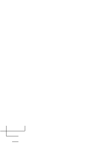
Figure 1: Shifted Young diagram of $\lambda=(4,2,1)$

The shifted Young diagram is given by a collection of boxes with coordinates

$$\left\{\left(i,j\right)\mid i=1,...,l(\lambda),\text{ }i\leq j\leq\lambda_{i}+i-1\right\}.$$ (6.2)

A shifted plane partition $\Pi$ of shape $\lambda$ is determined by the sequence $(...,.\pi_{-1},\pi_{0},\pi_{1},...)$, where $\pi_{0}$ the 2d- partition on the main diagonal and $\pi_{k}$ is the 2d- partition on the diagonal shifted by an integer $k$. All diagonal partitions are strict 2d- partitions forming altogether a shifted plane partition with the property

$$...\subset\pi_{-1}\subset\pi_{0}\supset\pi_{1}\supset...$$ (6.3)

For illustration, see the example

$$\pi_{-2}=\left(3\right)$$ , , ,

, , .

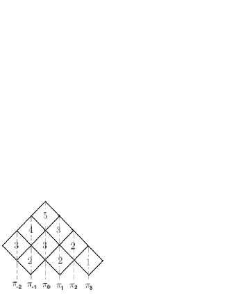
Figure 2: A strict plane partition

Property of Schur function for strict partition
The shifted topological vertex is defined by using skew Schur $P$ and $Q$ functions [20], [22]. These are symmetric functions that appear in topological amplitudes and are defined by a sequence of polynomials $P_{\lambda}(x_{1},x_{2},...x_{n})$, $n\in N$, with the property

$$P_{\lambda/\mu}(x_{1},\cdots x_{n})=\left\{\begin{array}[]{c}\sum\limits_{T}x^{T}\qquad\lambda\supset\mu\\ 0\qquad\text{otherwise}\end{array}\right.$$ (6.4)

where the sum is over all shifted Young tableaux of shape $\lambda/\mu$. The skew Schur function $Q_{\lambda/\mu}$ is related to $P_{\lambda/\mu}$ as in eqs(3.9-3.10). We also have

$$\sum_{\text{ strict }\lambda}Q_{\lambda}(x)P_{\lambda}(y)=\prod\limits_{i,j}\left(\frac{1+x_{i}y_{j}}{1-x_{i}y_{j}}\right).$$ (6.5)

The relation between the Schur function $P_{\lambda}$ for strict partition $\lambda$ that we have used hereabove and the usual Schur functions $S_{\tilde{\lambda}}$ for the double partition $\tilde{\lambda}$ is given by

$$S_{\tilde{\lambda}}(t)=2^{-l(\lambda)}P_{\lambda}^{2}(\frac{t}{2})\text{ ,}$$ (6.6)

where $\frac{t}{2}$ is $(\frac{t_{1}}{2},\frac{t_{3}}{2},\frac{t_{5}}{2},\cdots)$ and $P_{\lambda}(\frac{t}{2})=P_{\lambda}(\frac{t_{1}}{2},\frac{t_{3}}{2},\frac{t_{5}}{2},\cdots)$. Notice that the double partition $\tilde{\lambda}$ in Frobenuis notation reads in terms of the strict partition $\lambda=(n_{1},n_{2},\cdots,n_{k})$ as:

$$\tilde{\lambda}=(n_{1},n_{2},\cdots,n_{k}\mid n_{1}-1,n_{2}-1,\cdots,n_{k-1}-1)\text{ .}$$ (6.7)

References

[1] M. Aganagic, A. Klemm, M. Marino, C. Vafa, The
Topological Vertex, Commun. Math. Phys. 254 (2005) 425-478,
hep-th/0305132.
[2] A. Iqbal, A-K Kashani-Poor, The Vertex on a Strip, hep-th/0410174, Instanton Counting and Chern-Simons Theory, Adv.
Theor. Math. Phys. 7 (2004) 457-497, hep-th/0212279.
[3] Andrei Okounkov, Nikolai Reshetikhin, Cumrun Vafa, Quantum Calabi-Yau and Classical Crystals hep-th/0309208.
[4] Lalla Btissam Drissi, Houda Jehjouh, El Hassan Saidi, Non Planar Topological 3-Vertex Formalism, Nucl.Phys.B804:307-341,2008,
arXiv:0712.4249, [hep-th],
Lalla Btissam Drissi, Houda Jehjouh, El Hassan Saidi, Topological
String on Toric CY3s in Large Complex Structure Limit, Lab/UFR-HEP-0807-rev/GNPHE-0807-rev, To appear in Nuclear Phys B (2008),
arXiv:0812.0526.
[5] T. Graber and E. Zaslow, Open string Gromov-Witten
invariants: Calculations and a mirror ’theorem’, arXiv:hep-th/0109075.
[6] M. Aganagic, A. Klemm, and C. Vafa, “Disk Instantons, Mirror Symmetry and the Duality Web,”
hep-th/0105045.
[7] D. Karp, C. Liu, M. Marino, The local Gromov-Witten
invariants of configuration of rational curves, Geometry Topology
Monographs 10 (2006) 115-168.
[8] Amer Iqbal, Can Kozcaz, Cumrun Vafa, The Refined
Topological Vertex hep-th/0701156.