On the computational complexity of solving stochastic mean-payoff games

Abstract

We consider some well known families of two-player, zero-sum, turn-based, perfect information games that can be viewed as specical cases of Shapley’s stochastic games. We show that the following tasks are polynomial time equivalent:

• Solving simple stochastic games,

• solving stochastic mean-payoff games with rewards and probabilities given in unary, and

• solving stochastic mean-payoff games with rewards and probabilities given in binary.

1 Introduction

We consider some well known families of two-player, zero-sum, turn-based, perfect information games that can be viewed as specical cases of Shapley’s stochastic games [12]. They have appeared under various names in the literature in the last 50 years and variants of them have been rediscovered many times by various research communities. For brevity, in this paper we shall refer to them by the name of the researcher who first (as far as we know) singled them out.

• Condon games [5] (a.k.a. simple stochastic games). A Condon game is given by a directed graph $G=(V,E)$ with a partition of the vertices into $V_{1}$ (vertices beloning to Player 1, $V_{2}$ (vertices belonging to Player 2), $V_{R}$ (random vertices), and a special terminal vertex 1. Vertices of $V_{R}$ have exactly two outgong arcs, the terminal vertex 1 has none, while all vertices in $V_{1},V_{2}$ have at least one outgoing arc. Between moves, a pebble is resting at one of the vertices $u$. If $u$ belongs to a player, this player should strategically pick an outgoing arc from $u$ and move the pebble along this edge to another vertex. If $u$ is a vertex in $V_{R}$, nature picks an outgoing arc from $u$ uniformly at random and moves the pebble along this arc. The objective of the game for Player 1 is to reach 1 and should play so as to maximize his probability of doing so. The objective for Player 2 is to prevent Player 1 from reaching 1.

• Gillette games [7]. A Gillette game $G$ is given by a finite set of states $S$, partioned into $S_{1}$ (states belonging to Player 1) and $S_{2}$ (states belonging to Player 2). To each state $u$ is associated a finite set of possible actions. To each such action is associated a real-valued reward and a probability distribution on states. At any point in time of play, the game is in a particular state $i$. The player to move chooses an action strategically and the corresponding award is paid by Player 2 to Player 1. Then, nature chooses the next state at random according to the probability distribution associated with the action. The play continues forever and the accumulated reward may therefore be unbounded. Fortunately, there are ways of associating a finite payoff to the players in spite of this and more ways than one (so $G$ is not just one game, but really a family of games): For discounted Gillette games, we fix a discount factor $\beta\in(0,1)$ and define the payoff to Player 1 to be

  $$\sum_{i=0}^{\infty}\beta^{i}r_{i}$$

  where $r_{i}$ is the reward incurred at stage $i$ of the game. We shall denote the resulting game $G_{\beta}$. For undiscounted Gillette game we define the payoff to Player 1 to be the limiting average payoff

  $$\liminf_{n\rightarrow\infty}(\sum_{i=0}^{n}r_{i})/(n+1).$$

  We shall denote the resulting game $G_{1}$.

Undiscounted Gillette games have recently been referred to as stochastic mean-payoff games in the computer science literature [2]. A natural restriction of Gillette games is to deterministic transitions (i.e., all probability distributions put all probability mass on one state). This class of games has been studied in the computer science literature under the names of cyclic games [8] and mean-payoff games [13].

A strategy for a game is a (possibly randomized) procedure for selecting which arc or action to take, given the history of the play so far. A pure, positional strategy is the very special case of this where the choice is deterministic and only depends on the current vertex (or state), i.e., a pure, positional strategy is simply a map from vertices (for Gillette games, states) to vertices (for Gillette games, actions).

A strategy $x^{*}$ for Player 1 is said to be optimal if for all vertices (states) $i$ it holds that,

$$\inf_{y\in S_{2}}\mu^{i}(x^{*},y)\geq\sup_{x\in S_{1}}\inf_{y\in S_{2}}\mu^{i}(x,y)$$ (1)

where $S_{1}$ $(S_{2})$ is the set of strategies for Player 1 (Player 2) and $\mu^{i}(x,y)$ is the probability that Player 1 will end up in 1 (for the case of Condon games) or the expected payoff of Player 1 (for the case of Gillette games) when players play using the strategy profile $(x,y)$ and the play starts in vertex (state) $i$. Similarly, a strategy $y^{*}$ for Player 2 is said to be optimal if

$$\sup_{x\in S_{1}}\mu^{i}(x,y^{*})\leq\inf_{y\in S_{2}}\sup_{x\in S_{1}}\mu^{i}(x,y).$$ (2)

For all games described here, a proof of Liggett and Lippman [10] (fixing a bug of a proof of Gillette [7]) shows that there are optimal, pure, positional strategies and that a pair of such strategies form an exact Nash equilibrium of the game. These facts imply that when testing whether conditions (1) and (2) holds, it is enough to take the inifima and suprema over the finite set of pure, positional strategies of the players.

In this paper, we consider solving games. By solving a game we mean the task of computing a pair of optimal pure, positional strategies, given a description of the game as input. To be able to finitely represent the games, we assume that the discount factor, rewards and probabilities are rational numbers and given as fractions.

It is well known that Condon games can be seen as a special case of undiscounted Gillette games (as described in the proof of Lemma 4 below), but a priori, solving Gillette games could be harder. A recent paper by Chatterjee and Henzinger [2] shows that solving so-called stochastic parity games [1, 3] reduces to solving undiscounted Gillette games. This motivates the study of the complexity of the latter task. We show that the extra expressive power (compared to Condon games) of having rewards during the game in fact does not change the computational complexity of solving the games. More precisely, our main theorem is:

Theorem 1.

The following tasks are polynomial time equivalent:

1. Solving Condon games (a.k.a.., simple stochastic games)

2. Solving undiscounted Gillette games (a.k.a, stochastic mean-payoff games) with rewards and probabilities represented in binary notation.

3. Solving undiscounted Gillette games with rewards and probabilities represented in unary notation.

4. Solving discounted Gillette games with discount factor, rewards and probabilities represented in binary notation.

In particular, there is a pseudopolynomial time algorithm for solving undiscounted Gillette games if and only if there is a polynomial time algorithm for this task. The theorem follows from the Lemmas 2,3,4 below and the fact that solving games with numbers in the input represented in unary trivially reduces to solving games with numbers in the input represented in binary. The proof techniques are fairly standard (although coming from two different communities), but we find it worth pointing out that they together imply the theorem above since it is relevant, did not seem to be known, and may even be considered slightly surprising, as deterministic undiscounted Gillette games can be solved in pseudopolynomial time [8, 13], while solving them in polynomial time remains a challenging open problem. An even more challenging problem is solving simple stochastic games in polynomial time, so our theorem may be interpreted as a hardness result. Note that a “missing bullet” in the theorem is solving discounted Gillette games given in unary notation. It is in fact known that this can be done in polynomial time (even if only the discount factor is given in unary while rewards and probabilities are given in binary), see Littman [11, Theorem 3.4].

2 Proofs

Lemma 1.

Let $G$ be a Gillette game with $n$ states and all transition probabilities and rewards being fractions with integral numerators and denominators, all of absolute value at most $M$. Let $\beta^{*}=1-((n!)^{2}2^{2n+3}M^{2n^{2}})^{-1}$ and let $\beta\in[\beta^{*},1]$. Then, any optimal pure stationary strategy (for either player) in the discounted Gillette game $G_{\beta}$ is also an optimal strategy in the undiscounted Gillette game $G_{1}$.

Proof.

The fact that some $\beta^{*}$ with the desired property exists is explicit in the proof of Theorem 1 of Liggett and Lippman [10]. Here, we derive a concrete value for $\beta^{*}$. From the proof of Liggett and Lippman, we have that for $x^{*}$ to be an optimal pure stationary strategy (for Player 1) in $G_{1}$, it is sufficient to be an optimal pure stationary strategy in $G_{\beta}$ for all values of $\beta$ sufficiently close to $1$, i.e., to satisfy the inequalities

$$\min_{y\in S^{\prime}_{2}}\mu^{i}_{\beta}(x^{*},y)\geq\max_{x\in S^{\prime}_{1}}\min_{y\in S^{\prime}_{2}}\mu^{i}_{\beta}(x,y)$$

for all states $i$ and for all values of $\beta$ sufficiently close to $1$, where $S^{\prime}_{1}$ ($S^{\prime}_{2}$) is the set of pure, positional, strategies for Player 1 (2) and $\mu^{i}_{\beta}$ is the expected payoff when game starts in position $i$ and the discount factor is $\beta$. Similarly, for $y^{*}$ to be an optimal pure stationary strategy (for Player 1) in $G_{2}$, it is sufficient to be an optimal pure stationary strategy in $G_{\beta}$ for all values of $\beta$ sufficiently close to $1$, i.e., to satisfy the inequalities

$$\max_{x\in S^{\prime}_{1}}\mu^{i}_{\beta}(x,y^{*})\leq\min_{y\in S^{\prime}_{2}}\max_{x\in S^{\prime}_{1}}\mu^{i}_{\beta}(x,y).$$

So, we can prove the lemma by showing that for all states $i$ and all pure stationary strategies $x,y,z,u$, the sign of $\mu^{i}_{\beta}(x,y)-\mu^{i}_{\beta}(z,u)$ is the same for all $\beta\geq\beta^{*}$. For fixed strategies $x,y$ we have that $v_{i}=\mu^{i}_{\beta}(x,y)$ is the expected total reward in a discounted Markov process and is therefore given by the formula (see [9])

$$v=(I-\beta Q)^{-1}r,$$ (3)

where $v$ is the vector of $\mu_{\beta}(x,y)$ values, one for each state, $Q$ is the matrix of transition probabilities and $r$ is the vector of rewards (note that for fixed positional strategies $x,y$, rewards can be assigned to states in the natural way). Let $\gamma=1-\beta$. Then, (3) is a system of linear equations in the unknowns $v$, where each coefficient is of the form $a_{ij}\gamma+b_{ij}$ where $a_{ij},b_{ij}$ are rational numbers with numerators with absolute value bounded by $2M$ and with denominators with absolute value bounded by $M$. By multiplying the equations with all denominators, we can in fact assume that $a_{ij},b_{ij}$ are integers of absolute value less than $2M^{n}$. Solving the equations using Cramer’s rule, we may write an entry of $v$ as a quotient between determinants of $n\times n$ matrices containing terms of the form $a_{ij}\gamma+b_{ij}$. The determinant of such a matrix is a polynomial in $\gamma$ of degree $n$ with the coefficient of each term being of absolute value at most $n!(2M^{n})^{n}=n!2^{n}M^{n^{2}}$. We denote these two polynomials $p_{1},p_{2}$. Arguing similarly about $\mu_{\beta}(z,u)$ and deriving corresponding polynomials $p_{3},p_{4}$, we have that $\mu^{i}_{\beta}(x,y)-\mu^{i}_{\beta}(z,u)\geq 0$ is equivalent to $p_{1}(\gamma)/p_{2}(\gamma)-p_{3}(\gamma)/p_{4}(\gamma)\geq 0$, i.e., $p_{1}(\gamma)p_{4}(\gamma)-p_{3}(\gamma)p_{2}(\gamma)\geq 0$. Letting $q(\gamma)=p_{1}(\gamma)p_{4}(\gamma)-p_{3}(\gamma)p_{2}(\gamma)$, we have that $q$ is a polynomial in $\gamma$, with integer coefficients, all of absolute value at most $R=2(n!)^{2}2^{2n}M^{2n^{2}}$. Since $1-\beta^{*}<1/(2R)$, the sign of $q(\gamma)$ is the same for all $\gamma\leq 1-\beta^{*}$, i.e., for all $\beta\geq\beta^{*}$. This completes the proof. ∎

Lemma 2.

Solving undiscounted Gillette games (with binary representation of rewards and probabilities) polynomially reduces to solving discounted Gillette games (with binary representation of discount factor, rewards, and probabilities).

Proof.

This follows immediately from Lemma 1 by observing that the binary representation of the number $\beta^{*}=1-((n!)^{2}2^{2n+3}M^{2n^{2}})^{-1}$ has length polynomial in the size of the representation of the game. ∎

Lemma 3.

Solving discounted Gillette game (with binary representation of discount factor, rewards, and probabilities) polynomially reduces to solving Condon games.

Proof.

Zwick and Paterson [13] considered solving deterministic discounted Gillette games, i.e., Gillette games where the action deterministically determines the transition taken. It is natural to try to generalize their reduction so that it also works for general discounted Gillette games. Since Condon games allows for vertices making random choices, a natural attempt is to simply simulate a stochastic transition by such random vertices. Such a generalization is made even easier by the fact that Zwick and Paterson proved that solving “augmented” Condon games where random vertices are allowed to take choices given by arbitrary discrete distributions with rational probability weights (represented in binary) is polynomially equivalent to solving “plain” Condon games. We find that the reduction outlined above is indeed correct, even though the correctness proof of Zwick and Paterson has to be modified slightly compared to their proof. The details follow.

We are given as input a Gillette game form $G$ and a discount factor $\beta$ and must produce an augmented Condon game $G^{\prime}$ whose solution yields the solution to the Gillette game $G_{\beta}$. First, we affinely scale and translate all rewards of $G$ so that they are in the interval $[0,1]$. This does not influence the optimal strategies. Vertices of $G^{\prime}$ include all states of $G$ (belonging to the same player in $G^{\prime}$ as in $G$), and, in addition, a random vertex $w_{u,A}$ for each possible action $A$ of each state $u$ of $G$. We also add a “trapping” vertex 0 with a single arc to itself. It does not matter which player it belongs to. We construct the arcs of $G^{\prime}$ by adding, for each (state,action) pair $(u,A)$ the “gadget” indicated in Figure 1.

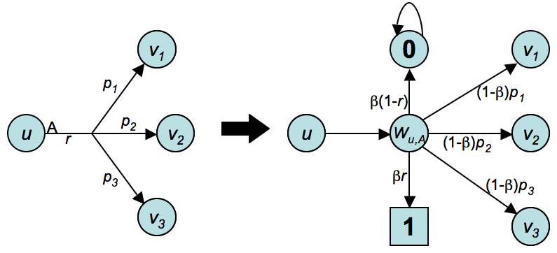
Figure 1: Reducing discounted Gillette games to Condon games

To be precise, if the action has reward $r$ and leads to states $v_{1},v_{2},\ldots,v_{k}$ with probability weights $p_{1},p_{2},\ldots,p_{k}$, we include in $G^{\prime}$ an arc from $u$ to $w_{u,A}$, arcs from $w_{u,A}$ to $v_{1},\ldots,v_{k}$ with probability weights $(1-\beta)p_{1},\ldots,(1-\beta)p_{k}$, an arc from $w_{u,A}$ to 0 with probability weight $\beta(1-r)$ and finally an arc from $w_{u,A}$ to the terminal 1 with probability weight $\beta r$.

There is clearly a 1-1 correspondence between pure stationary strategies in $G$ and in $G^{\prime}$. Thus, we are done if we show that the optimal strategies coincide. To see this, fix a strategy profile for the two players and consider play starting in any vertex $u$. By construction, if the expected reward of the play in $G$ is $h$, the probability that the play in $G^{\prime}$ ends up in 1 is exactly $\beta h$. Therefore, the two games are strategically equivalent. ∎

Lemma 4.

Solving Condon games polynomially reduces to solving undiscounted Gillette games with unary representation of rewards and probabilities.

Proof.

We are given a Condon game $G$ (a “plain” one, using the terminology of the previous proof) and must construct an undiscounted Gillette game $G^{\prime}$. States of $G^{\prime}$ will coincide with vertices of $G$, with the states of $G^{\prime}$ including the special terminals 1. Vertices $u$ belonging to a player in $G$ belongs to the same player in $G^{\prime}$. For each outgoing arc of $u$, we add an action in $G^{\prime}$ with reward 0, and with a deterministic transition to the endpoint of the arc of $G$. Random vertices of $G$ can be assigned to either player in $G^{\prime}$, but he will only be given a single “dummy choice”: If the random vertex has arcs to $v_{1}$ and $v_{2}$, we add a single action in $G^{\prime}$ with reward $0$ and transitions into $v_{1}$, $v_{2}$, both with probability weight $1/2$. The terminal 1 can be assigned to either player in $G^{\prime}$, but again he will be given only a dummy choice: We add a single action with reward 1 from 1 and with a transition back into 1 with probability weight $1$.

There is clearly a 1-1 correspondence between pure stationary strategies in $G$ and strategies in $G^{\prime}$. Thus, we are done if we show that the optimal strategies coincide. To see this, fix a strategy profile for the two players and consider play starting in any vertex $u$. By construction, if the probability of the play ending up in 1 in $G$ is $q$, the expected limiting average reward of the play in $G^{\prime}$ is also $q$. Therefore, the two games are strategically equivalent, and we are done. ∎

3 Open problems

Undiscounted Gillette games can be seen as generalizations of Condon games and yet they are computationally equivalent. It is interesting to ask if further generalizations of Gillette games are also equivalent to solving Condon games. It seems natural to restrict attention to cases where it is known that optimal, positional strategies exists. This precludes general stochastic games (but see [4]). An interesting class of games generalizing undiscounted Gillette games was considered by Filar [6]. Filar’s games allow simultaneous moves by the two players. However, for any position, the probability distribution on the next position can depend on the action of one player only. Filar shows that his games are guaranteed to have optimal, positional strategies. The optimal strategies are not necessarily pure, but the probabilities they assign to actions are guaranteed to be rational numbers if rewards and probabilities are rational numbers. So, we ask: Is solving Filar games polynomial time equivalent to solving Condon games?

References

- [1] K. Chatterjee, M. Jurdziński, and T.A. Henzinger. Simple stochastic parity games. In CSL: Computer Science Logic, Lecture Notes in Computer Science 2803, pages 100–113. Springer, 2003.
- [2] Krishnendu Chatterjee and Thomas A. Henzinger. Reduction of stochastic parity to stochastic mean-payoff games. Inf. Process. Lett., 106(1):1–7, 2008.
- [3] Krishnendu Chatterjee, Marcin Jurdziński, and Thomas A. Henzinger. Quantitative stochastic parity games. In SODA ’04: Proceedings of the fifteenth annual ACM-SIAM symposium on Discrete algorithms, pages 121–130, Philadelphia, PA, USA, 2004. Society for Industrial and Applied Mathematics.
- [4] Krishnendu Chatterjee, Rupak Majumdar, and Thomas A. Henzinger. Stochastic limit-average games are in EXPTIME. International Journal of Game Theory, to appear.
- [5] Anne Condon. The complexity of stochastic games. Information and Computation, 96:203–224, 1992.
- [6] J.A. Filar. Ordered field property for stochastic games when the player who controls transitions changes from state to state. Journal of Optimization Theory and Applications, 34:503–513, 1981.
- [7] D. Gillette. Stochastic games with zero stop probabilities. In M. Dresher, A.W. Tucker, and P. Wolfe, editors, Contributions to the Theory of Games III, volume 39 of Annals of Mathematics Studies, pages 179–187. Princeton University Press, 1957.
- [8] V.A. Gurvich, A.V. Karzanov, and L.G. Khachiyan. Cyclic games and an algorithm to find minimax cycle means in directed graphs. USSR Computational Mathematics and Mathematical Physics, 28:85–91, 1988.
- [9] Ronald A. Howard. Dynamic Programming and Markov Processes. M.I.T. Press, 1960.
- [10] Thomas M. Liggett and Steven A. Lippman. Stochastic games with perfect information and time average payoff. SIAM Review, 11(4):604–607, 1969.
- [11] Michael Lederman Littman. Algorithms for sequential decision making. PhD thesis, Brown University, Department of Computer Science, 1996.
- [12] L.S. Shapley. Stochastic games. Proc. Nat. Acad. Science, 39:1095–1100, 1953.
- [13] Uri Zwick and Mike Paterson. The complexity of mean payoff games on graphs. Theor. Comput. Sci., 158(1-2):343–359, 1996.