Statistical Analysis of future Neutrino Mass Experiments including Neutrino-less Double Beta Decay
 

We perform a statistical analysis with the prospective results of future experiments on neutrino-less double beta decay, direct searches for neutrino mass (KATRIN) and cosmological observations. Realistic errors are used and the nuclear matrix element uncertainty for neutrino-less double beta decay is also taken into account. Three benchmark scenarios are introduced, corresponding to quasi-degenerate, inverse hierarchical neutrinos, and an intermediate case. We investigate to what extend these scenarios can be reconstructed. Furthermore, we check the compatibility of the scenarios with the claimed evidence of neutrino-less double beta decay.

1 Introduction

Neutrino mass and lepton mixing represent an unambiguous proof that the Standard Model (SM) of elementary particles is incomplete. Various experiments with solar [1], atmospheric [2] and man-made [3, 4] neutrino sources imply non-trivial lepton mixing angles, as well as non-zero and non-degenerate neutrino masses. Their values are extremely suppressed with respect to the masses of the other (electrically charged) fermions of the SM. The most prominent and often studied mechanism to explain the smallness of neutrino masses is the see-saw mechanism [5]. The neutrino mass scale is here inversely proportional to the scale of its origin. In addition, lepton number violation is predicted: neutrinos are Majorana particles. Searching for this property will be a crucial test of the see-saw mechanism, but also of other mechanisms leading to small Majorana neutrino masses. Possible phenomenological consequences of lepton number violation are the generation of the baryon asymmetry of the Universe [6] or, at low energies, neutrino-less double beta decay (0$\nu\beta\beta$) [7]. This decay of certain nuclei, $(A,Z)\rightarrow(A,Z+2)+2\,e^{-}$, which has not yet been observed, clearly violates lepton number by two units, and is intensively searched for [7]. We will assume here that light Majorana neutrinos are exchanged in the diagram responsible for 0$\nu\beta\beta$. In this case, the amplitude for this process is proportional to the coherent sum

$$m_{ee}\equiv\sum\limits_{i=1}^{3}U_{ei}^{2}\,m_{i}\,,$$ (1)

where $m_{i}$ are the individual neutrino masses and $U$ is the leptonic mixing, or Pontecorvo-Maki-Nakagawa-Sakata (PMNS), matrix. The absolute value of $m_{ee}$ is called the effective mass. The entries $U_{ei}$ can be written as $U_{e1}=\cos\theta_{12}\,\cos\theta_{13}$, $U_{e2}=\sin\theta_{12}\,\cos\theta_{13}\,e^{i\alpha}$ and $U_{e3}=\sin\theta_{13}\,e^{i\beta}$, where $\alpha$ and $\beta$ are two currently unknown “Majorana phases” and $\theta_{12,13}$ are mixing angles. While $\theta_{13}$ is constrained mainly by short-baseline reactor experiments, $\theta_{12}$ is probed by solar and long-baseline reactor neutrino experiments. Their current best-fit values as well as $1\sigma$ and $3\sigma$ ranges can be obtained from three-flavor fits, the result being [8]

$$\sin^{2}\theta_{12}=0.32\,(\pm 0.02)^{+0.08}_{-0.06}~{},~{}\sin^{2}\theta_{13}=0^{+0.019,\,0.050}\,.$$ (2)

In what regards the neutrino masses, for a normal ordering one has $m_{3}>m_{2}>m_{1}$ with $m_{2}^{2}=m_{1}^{2}+\mbox{$\Delta m^{2}_{\odot}$}$ and $m_{3}^{2}=m_{1}^{2}+\mbox{$\Delta m^{2}_{\rm A}$}$. In case of an inverted ordering we have $m_{2}>m_{1}>m_{3}$ with $m_{2}^{2}=m_{3}^{2}+\mbox{$\Delta m^{2}_{\odot}$}+\mbox{$\Delta m^{2}_{\rm A}$}$ and $m_{1}^{2}=m_{3}^{2}+\mbox{$\Delta m^{2}_{\rm A}$}$. Here $\Delta m^{2}_{\odot}$ and $\Delta m^{2}_{\rm A}$ are mass-squared differences with best-fit values and $3\sigma$ ranges $(7.9^{+1.1}_{-0.9})\cdot 10^{-5}$ eV² and $(2.6^{+0.6}_{-0.6})\cdot 10^{-3}$ eV², respectively [8]. Quasi-degenerate neutrino masses occur when $m_{1,2,3}^{2}\gg\mbox{$\Delta m^{2}_{\rm A}$},\mbox{$\Delta m^{2}_{\odot}$}$. If neutrinos are Majorana particles, all low energy neutrino phenomenology can be described by the neutrino mass matrix $m_{\nu}=U^{\ast}\,m_{\nu}^{\rm diag}\,U^{\dagger}$. It contains nine physical parameters. Seven out of the nine parameters of the neutrino mass matrix appear in $\left|m_{ee}\right|$. Therefore, it contains a large amount of information, in particular if complementary measurements of some of the other parameters exist. We also note that all parameters of $m_{\nu}$ which do not influence neutrino oscillations show up in the effective mass. Those are the the Majorana phases and, in particular, the individual neutrino masses (neutrino oscillations are only sensitive to mass-squared differences). For a review on the dependence of $\left|m_{ee}\right|$ on the various neutrino parameters see refs. [7, 9, 10] and references therein. In the present paper, in contrast to other works statistically analyzing future neutrino mass measurements including 0$\nu\beta\beta$ [14, 11, 12, 13, 15, 16, 17], we focus on the neutrino mass scale, i.e. the value of the smallest neutrino mass. To this end we define three natural benchmark scenarios and investigate how future experiments may be able to constrain them. Our goal here is to combine as much mass-related information as possible.

2 Observables related to neutrino mass

Currently the strongest experimental limits on the half-life of neutrino-less double beta decay are (all at 90 $\%$ C.L.) $1.9\cdot 10^{25}$ y for ⁷⁶Ge [19] (see also [20]), T${}_{1/2}\geq 3.0\cdot 10^{24}$ y for ¹³⁰Te [21], T${}_{1/2}\geq 5.8\cdot 10^{23}$ y for ¹⁰⁰Mo and T${}_{1/2}\geq 2.1\cdot 10^{23}$ y for ⁸²Se [22]. The existing limits on T_1/2 will be improved considerably (by two orders of magnitude or more) in the near future by various experiments [7]. The uncertainty in nuclear matrix element (NME) calculations is a serious problem to translate these bounds into upper limits on the effective mass [23, 17]. We will take into account in particular this uncertainty in our analysis. Depending on the nuclei and NME, the current limit on the effective mass as extracted from the half-lifes given above lies between several tenths of and a few eV. This has to be compared with the predictions which can be made for the effective mass. Inserting the known ranges of the oscillation parameters, and varying the unknown parameters within their allowed ranges, one can generate plots as the ones in fig. 1.

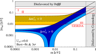
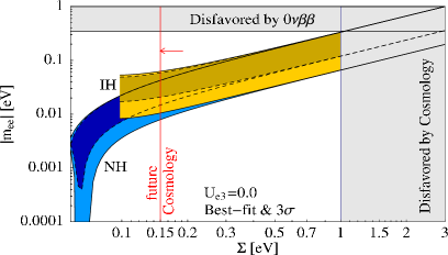
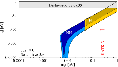
Figure 1: The effective mass as a function of the smallest neutrino mass, the sum of neutrino masses $\Sigma$ and the kinematic neutrino mass $m_{\beta}$. The value $U_{e3}=0$ and the current 3$\sigma$ ranges of the other oscillation parameters have been used.

They display (for $U_{e3}=0$) the effective mass as a function of the smallest neutrino mass, the sum of neutrino masses

$$\Sigma\equiv\sum\limits_{i=1}^{3}m_{i}$$ (3)

and the kinematic neutrino mass

$$m_{\beta}\equiv\sqrt{\sum\limits_{i=1}^{3}|U_{ei}|^{2}\,m_{i}^{2}}\,.$$ (4)

The latter two quantities can be measured through cosmological observations [24] and experiments like KATRIN [25], respectively. The latter experiment has a $5\sigma$ discovery potential of 0.35 eV for $m_{\beta}$, and a null result will lead to a 90 $\%$ C.L. limit of 0.2 or 0.17 eV [26]. In the sensitivity range of KATRIN, the relation $3\,m_{\beta}=\Sigma$ holds to a very good precision. Cosmology is expected to probe values of $\Sigma$ down to the 0.1 eV range [24] (to be specific, we take a value of 0.15 eV in fig. 1). To achieve such impressive results, one takes advantage of future observations of weak gravitational lensing of galaxies, and the cosmic microwave background or detailed analyses of the 21 cm hydrogen emission lines at high redshift. It is fair to say that a conservative limit on $\Sigma$ is 1 eV. This value corresponds roughly to the bound obtained from WMAP 5-year data alone [28]. Recall that neutrino mass bounds from cosmology depend strongly on the data sets, the priors and the model, i.e., adding parameters which are degenerate with neutrino masses will relax the bounds, see, e.g., [29]. Finally, current limits for $m_{\beta}$ are 2.3 eV [27].

The blue and yellow bands in fig. 1 correspond to the normal and inverted mass ordering of the neutrinos, respectively. The darker areas in the blue and yellow bands are obtained when the oscillation parameters are fixed to their best-fit values and only the Majorana phases are varied. The lighter areas correspond to the $3\sigma$ ranges of the oscillation parameters. Note that this broadening is very weak for the maximum value of $\left|m_{ee}\right|$ in the case of inverted mass ordering and for quasi-degenerate neutrinos. This is because the upper limits on $\left|m_{ee}\right|$ are roughly $\sqrt{\mbox{$\Delta m^{2}_{\rm A}$}}$ and $m_{3}$, respectively, and varying the oscillation parameters has very little impact. In the first plot of fig. 1, we have indicated three special values of $\left|m_{ee}\right|$ which correspond to the goals of the three phases of the GERDA experiment (where a certain NME has been assumed, see [30] for details).

3 Statistical analysis

Now we will perform a statistical analysis to investigate how well it will be possible to reconstruct different realistic physical scenarios with upcoming neutrino mass experiments. Note that, since we want to investigate realistic situations, we concentrate only on cases that can be probed in the near future. For definiteness, we consider the inverted mass ordering and three different scenarios called ${\cal QD}$ (quasi-degenerate), ${\cal INT}$ (intermediate) and ${\cal IH}$ (inverted hierarchy) that are defined by different values of the smallest neutrino mass $m_{3}$. Note that the ${\cal QD}$ scenario would, to very large extent, also apply to a normal mass ordering. The hypothetical “true values” for the different observables in these scenarios are:

Scenario	$m_{3}$ [eV]	$\left|m_{ee}\right|$ [eV]	$m_{\beta}$ [eV]	$\Sigma$ [eV]
${\cal QD}$	0.3	$0.11-0.30$	0.30	0.91
${\cal INT}$	0.1	$0.04-0.11$	(0.11)	0.32
${\cal IH}$	0.003	$0.02-0.05$	(0.05)	(0.10)

We have used here the best-fit values for the oscillation parameters. The range for $\left|m_{ee}\right|$ originates from the variation of the Majorana phases $\alpha$ and $\beta$. Note that the KATRIN experiment will only be able to measure $m_{\beta}$ in the case of the ${\cal QD}$ scenario, while for ${\cal INT}$ and ${\cal IH}$ it will only provide an upper limit. The same is true for the measurement of $\Sigma$ in the ${\cal IH}$ scenario. These cases are indicated in the table by writing the respective values in brackets.

Let us now give a summary of the different experimental errors and theoretical uncertainties. Regarding the error on the effective mass in $0\nu\beta\beta$, we have to distinguish between experimental and “theoretical uncertainties”, where the latter result from the NME uncertainty. The experimental error can be included by noting that the decay width depends quadratically on the effective mass. Thus,

$$\sigma(\mbox{$\left|m_{ee}\right|$}_{\rm exp})=\frac{|m_{ee}|_{\rm exp}}{2}\,\frac{\sigma(\Gamma_{\rm obs})}{\Gamma_{\rm obs}}\,,$$ (5)

where $|m_{ee}|_{\rm exp}$ is the measured value of the effective neutrino mass and $\sigma(\Gamma_{\rm obs})$ is the experimental error on the measured decay width $\Gamma_{\rm obs}$ for neutrino-less double beta decay. For definiteness, we choose the ratio of the latter two as

$$\frac{\sigma(\Gamma_{\rm obs})}{\Gamma_{\rm obs}}\simeq 23.3\%\,,$$ (6)

which is the value obtainable in the GERDA experiment [30]. We combine, similarly to the procedure developed in ref. [11], the experimental error with the theoretical NME error via

$$\sigma(\mbox{$\left|m_{ee}\right|$})=(1+\zeta)\,\left(\mbox{$\left|m_{ee}\right|$}+\sigma(\mbox{$\left|m_{ee}\right|$}_{\rm exp})\right)-\mbox{$\left|m_{ee}\right|$}\,,$$ (7)

where $\zeta\geq 0$ parameterizes the NME uncertainty and $\sigma(\mbox{$\left|m_{ee}\right|$}_{\rm exp})$ is given in eq. (5). Following ref. [14], we define a covariance matrix

$$S_{ab}\equiv\delta_{ab}\,\sigma^{2}(a)+\sum_{i}\frac{\partial T_{a}}{\partial x_{i}}\,\frac{\partial T_{b}}{\partial x_{i}}\,\sigma^{2}_{i}\,,$$ (8)

where $T_{1}=\mbox{$\left|m_{ee}\right|$}$, $T_{2}=\Sigma$ and $T_{3}=m_{\beta}^{2}$. Furthermore, $\sigma^{2}(a)$ is the error on $T_{a}$, and $a$, $b$ label the entries in the covariance matrix. The $x_{i}$ are the oscillation parameters that enter $\left|m_{ee}\right|$ (and $m_{\beta}$, though in the observable range of $m_{\beta}$ they have basically no influence).The errors on the $T_{a}$ are given by eq. (7) as well as by $\sigma(m_{\beta}^{2})=0.025$  eV² [25, 26] and $\sigma(\Sigma)=0.05$ eV [24].

Defining $v_{a}=T_{a}-(T_{a})_{\rm exp}$, where $(T_{a})_{\rm exp}$ denotes the experimental value of $T_{a}$, our $\chi^{2}$-function to be minimized is

$$\chi^{2}=v^{T}\,S^{-1}\,v\,.$$

All oscillation parameters are set to their current best-fit values and their (symmetrized) standard deviations are determined from their 1$\sigma$-ranges, which is a good approximation for future 3$\sigma$-ranges. Anyway, the impact of different numerical values here would not lead to qualitatively different results.We first minimize the $\chi^{2}$ from eq. (3) with respect to the Majorana phases $\alpha$ and $\beta$. The resulting function is $\chi^{2}_{\rm res}=\min_{\alpha,\beta}\chi^{2}$. We then continue by plotting the resulting $1\sigma$, $2\sigma$ and $3\sigma$ ranges for the smallest neutrino mass $m_{3}$ determined by setting $\Delta\chi^{2}=\chi^{2}_{\rm res}-\chi^{2}_{\rm res,min}$ equal to 1, 4 and 9. This corresponds to a $\chi^{2}$-function with one free parameter (namely $m_{3}$). $|m_{ee}|_{\rm exp}$ is the assumed measured value of $\left|m_{ee}\right|$, on which the reconstructed range of $m_{3}$ depends. The minimum in the $|m_{ee}|_{\rm exp}$-$m_{3}$ plane is determined such that $\Delta\chi^{2}$ is zero in the true region of the corresponding scenario (e.g., $\cal QD$).

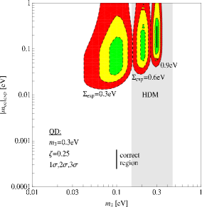
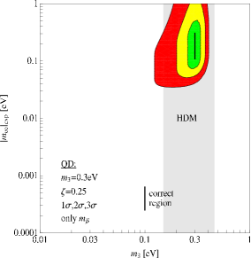
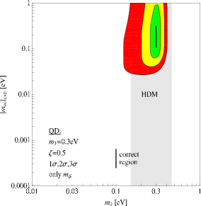
Figure 2: 1$\sigma$, 2$\sigma$ and 3$\sigma$ regions in the $m_{3}$-$\mbox{$\left|m_{ee}\right|$}_{\rm exp}$ plane for the ${\cal QD}$ scenario. The left column shows the correct (solid line) as well as two possible incorrect cosmological measurements (dashed lines). The less desirable case, namely only taking into account a KATRIN measurement, is shown in the plots on the right. The area denoted HDM is the range of $\left|m_{ee}\right|$ from the claim of part of the Heidelberg-Moscow collaboration.

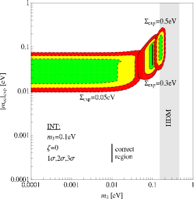
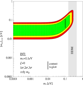
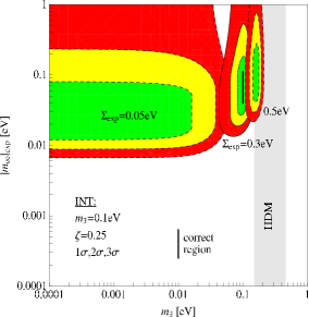
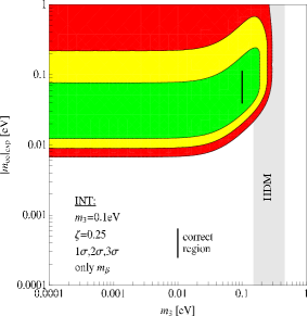
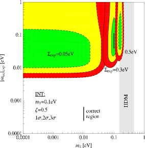
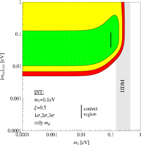
Figure 3: Same as fig. 2 for the ${\cal INT}$ scenario.

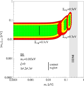
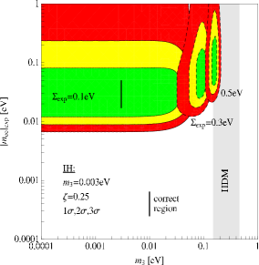
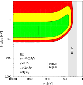
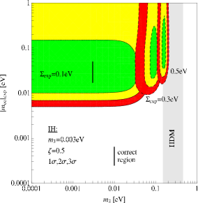
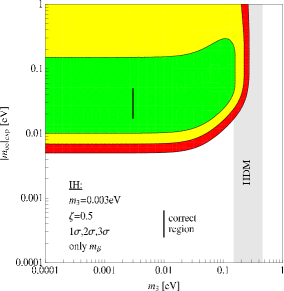
Figure 4: Same as fig. 2 for the ${\cal IH}$ scenario.

The results of our analysis are shown as the solid lines in the left column of figs. 2, 3 and 4. In all cases, we have calculated the result for a consistent measurement (i.e., $m_{\beta}$ and $\Sigma$ are measured at their true values in the corresponding scenarios). The NME uncertainties we have chosen are $\zeta=0$ (no uncertainty), 0.25 and 0.5. We have checked that values of $\zeta>0.5$ will lead to results not too much different from the ones for $\zeta=0.5$. The value $\zeta=0.25$ is a quite typical one, cf. refs. [23, 17]. This uncertainty arises from the highly non-trivial calculations of the nuclear part of the neutrino-less double beta decayprocess. Different methods, and even different Ansätze within the same framework, differ in their result, and their spread is commonly taken into account as “theoretical uncertainty”. Glancing at Fig. 5 in ref. [31], where the results of different methods of the NME calculation are compared for different nuclei including ⁷⁶Ge, one can indeed see that the spread of the respective values around their mean value is about 0.2. We conclude that the values we use are realistic and typical.

The true values of $\left|m_{ee}\right|$ and $m_{3}$ are marked by the vertical black lines. The plots illustrate how well we can reconstruct the different scenarios for the various values of NME uncertainty. Having a look at fig. 2, we see that the ${\cal QD}$ scenario can be reconstructed quite well, which is not surprising since in that case the KATRIN experiment as well as the cosmological measurement will provide a non-trivial signal. E.g., for $|m_{ee}|_{\rm exp}=0.20$ eV, the 1, 2 and 3$\sigma$ ranges for $m_{3}$ are $0.28-0.32$ eV, $0.27-0.33$ eV and $0.25-0.35$ eV, while the true value is 0.30 eV. Therefore, the reconstruction is quite accurate. This remains true also if the uncertainty in NME is non-zero because the plots are still narrow around the true value of $m_{3}$ (the numerical values suffer nearly no change) even though, with a larger NME uncertainty, also higher values of $|m_{ee}|_{\rm exp}$ are plausible. This is true for all three scenarios under consideration.

Similar statements hold for the ${\cal INT}$ scenario shown in fig. 3, even though $m_{\beta}$ cannot be measured now. However, because there will still be a measurement of $\Sigma$, we have sufficient information on the neutrino mass. In case the central measured value is $\mbox{$\left|m_{ee}\right|$}_{\rm exp}=0.08$ eV and $\zeta=0$ the ranges are $0.08-0.12$ eV at 1$\sigma$ and $0.05-0.15$ eV at 3$\sigma$. In case of $\zeta=0.5$ we find $0.08-0.12$ eV at 1$\sigma$ and $0.04-0.15$ eV at 3$\sigma$. The mass scale has now a $3\sigma$ uncertainty of 50 %, to be compared with roughly 15 % in the ${\cal QD}$ scenario.

For ${\cal IH}$, in turn, there is no measurement that gives information $m_{3}$. Hence, it is only possible to give an upper limit on the smallest neutrino mass, as illustrated by the long horizontal band in the left column of fig. 4. Note that this band corresponds to the yellow band marking the inverted mass ordering in the upper plot of fig. 1. This upper limit is almost trivial, i.e., it corresponds to the neutrino mass limit obtainable from 0$\nu\beta\beta$ alone. To give some numerical values, for $\mbox{$\left|m_{ee}\right|$}_{\rm exp}=0.04$ eV one would have the 1 (3)$\sigma$ ranges $m_{3}<0.03~{}(0.07)$ eV for $\zeta=0$ and for $\zeta=0.5$. Due to the bound on $\Sigma$, there is very little dependence on $\zeta$.

Up to now, the discussion has focused on the case in which all measurements are compatible. As an example for inconsistency we discuss here a possible clash between results from KATRIN and from cosmology. To this end we leave $(m_{\beta})_{\rm exp}$ equal to the true value of the corresponding scenario (new physics is not expected to influence $m_{\beta}$ [32]) and take values of $\Sigma_{\rm exp}$ which are smaller or larger than the true value. There are many scenarios or models in the literature which can lead to wrong values of $\Sigma$, see, e.g., refs. [33]. The result is shown by the areas within the dashed lines in the left columns of figs. 2-4. Having a look at ${\cal QD}$ first, we realize immediately that the physical range is reconstructed incorrectly. Hence, if there are systematic errors in the cosmological measurement, or unknown features in cosmology which we are not aware of, a wrong neutrino mass is reconstructed. In the ${\cal QD}$ case there is still information from KATRIN, which leads to a reconstructed neutrino mass at most one order away from the true value, even if the wrong $\Sigma$ is taken into account. For the ${\cal INT}$ scenario, however, there is no information from KATRIN. Consequently, it might be that a wrong upper limit on $m_{3}$ is concluded, as illustrated by the long band for $\Sigma_{\rm exp}=0.05$ eV in the upper left plot of fig. 3. This is an example wherein one could draw a wrong conclusion by taking the cosmological measurement at face value. As expected, even worse cases may exist for the ${\cal IH}$ scenario. E.g., in the upper left plot of fig. 4 one would, for $\Sigma_{\rm exp}=0.3$ eV, reconstruct a smallest neutrino mass of roughly 0.1 eV, to be compared with the true value of $m_{3}=0.003$ eV. For the ${\cal IH}$ scenario, one might not even realize that there is an inconsistency, since in that case, the KATRIN experiment can only provide an upper limit which is too far away from the true value of $m_{3}$.

One possible cross-check (or the possible consequence if one indeed finds that the results from KATRIN and from cosmology do not fit together) would be to dismiss the cosmological data altogether. We have also analyzed this case. Here, $S_{ab}$ from eq. (8) as well as $v_{a}$ would change from 3-dimensional to 2-dimensional objects while the rest of the procedure remains the same. The results for this analysis are plotted in the right columns of figs. 2-4, again for different values of the NME uncertainty. For ${\cal QD}$, the most optimal scenario, neglecting cosmology, would simply increase the errors in the determination of $m_{3}$: e.g., for $\mbox{$\left|m_{ee}\right|$}_{\rm exp}=0.20$ eV and $\zeta=0$ the ranges are $0.26-0.34$ eV at 1$\sigma$ and $0.16-0.41$ eV at 3$\sigma$, while for $\zeta=0.5$ we find $0.26-0.34$ eV at 1$\sigma$ and $0.13-0.41$ eV at 3$\sigma$. The NME uncertainty has now a slightly bigger impact, and the error on $m_{3}$ increases by a factor of three, since now it is about 50 % while it was roughly 15 % when $\Sigma$ has been included in the analysis. For the ${\cal INT}$ scenario, however, there is a major difference to the former case: since now there is no other measurement besides $|m_{ee}|_{\rm exp}$ providing information on $m_{3}$, we can only derive an upper limit instead of determining a certain range for $m_{3}$. This is indicated by the band in the upper right plot of fig. 3. Finally, for ${\cal IH}$, the limit on $m_{3}$ gets only slightly worse compared to the case of a $\Sigma$, which is too small to be measured. In this case there would not even be a real drawback in taking into account the KATRIN result only. It remains to be said that in all cases a higher uncertainty for the NME does not significantly modify the conclusions in what concerns the value of $m_{3}$. Finally, it is worth mentioning that if in ${\cal QD}$ scenarios the error on $\Sigma$ is decreased (increased), the obtained error on the neutrino mass is decreased (increased) by approximately the same factor.

With our analysis we can also compare the compatibility of our three benchmark scenarios with the range for $m_{3}$ of $0.15-0.46$ eV, calculated as the (global fit) $2\sigma$ range in ref. [16] from the claim in ref. [18]. We give the implied range for $m_{3}$ as the gray band in figs. 2, 3 and 4. We see that scenario ${\cal QD}$ is consistent with the claim, even for a measurement of $\Sigma=0.6$ eV, to be compared with the true value $\Sigma=0.9$ eV. The ${\cal INT}$ scenario (${\cal IH}$ scenario) is barely (very) incompatible for measured “true” values, but a too high value of $\Sigma_{\rm exp}$ can lead again to compatibility. We see that testing the claim and comparing it with cosmology is a non-trivial task (see also [17]).

4 Conclusions

In this work we have investigated possible constraints on the neutrino mass in future experiments. We assumed realistic errors on the observables, in particular for neutrino-less double beta decay. Then, we have checked how certain realistic benchmark scenarios, which correspond to different regimes for the smallest neutrino mass, can be reconstructed from future measurements. Furthermore, we have pointed out how wrong conclusions could be drawn from inconsistent results, i.e., if cosmology provides a wrong value for the sum of neutrino masses. In case of consistent measurements we may summarize as follows: typical $3\sigma$ errors for quasi-degenerate neutrino masses range from roughly 15 % (including $\Sigma$) to 50 % (excluding $\Sigma$), where NME uncertainties play a larger role in the latter case. Intermediate scale masses can also be determined with 50 % uncertainty. In case of an inverted hierarchy, the effective mass is constant for a large range of the smallest mass, which allows only to derive upper limits on it.

References

- [1] B. T. Cleveland et al., Astrophys. J. 496 (1998) 505. E. Nakano et al. [Belle Collaboration], Phys. Rev. D 73, 112002 (2006) [arXiv:hep-ex/0505017]. J. N. Abdurashitov et al. [SAGE Collaboration], J. Exp. Theor. Phys. 95 (2002) 181 [Zh. Eksp. Teor. Fiz. 122 (2002) 211] [arXiv:astro-ph/0204245]. J. N. Abdurashitov et al. [SAGE Collaboration], J. Exp. Theor. Phys. 95, 181 (2002) [Zh. Eksp. Teor. Fiz. 122, 211 (2002)] [arXiv:astro-ph/0204245]. W. Hampel et al. [GALLEX Collaboration], Phys. Lett. B 447, 127 (1999). M. Altmann et al. [GNO COLLABORATION Collaboration], Phys. Lett. B 616, 174 (2005) [arXiv:hep-ex/0504037]. B. Aharmim et al. [SNO Collaboration], Phys. Rev. C 75, 045502 (2007) [arXiv:nucl-ex/0610020]. C. Arpesella et al. [Borexino Collaboration], Phys. Lett. B 658, 101 (2008) [arXiv:0708.2251 [astro-ph]].
- [2] Y. Ashie et al. [Super-Kamiokande Collaboration], Phys. Rev. D 71, 112005 (2005) [arXiv:hep-ex/0501064].
- [3] S. Abe et al. [KamLAND Collaboration], Phys. Rev. Lett. 100, 221803 (2008) [arXiv:0801.4589 [hep-ex]].
- [4] M. H. Ahn et al. [K2K Collaboration], Phys. Rev. D 74, 072003 (2006) [arXiv:hep-ex/0606032]. P. Adamson et al. [MINOS Collaboration], Phys. Rev. D 77, 072002 (2008) [arXiv:0711.0769 [hep-ex]].
- [5] P. Minkowski, Phys. Lett. B 67, 421 (1977). T. Yanagida, in Proceedings of the Workshop on The Unified Theory and the Baryon Number in the Universe, KEK, Tsukuba, Japan, 1979, O. Sawada and A. Sugamoto (Editors), 95; S. L. Glashow, in Proceedings of the 1979 Cargèse Summer Institute on Quarks and Leptons, M. Lévy, J.-L. Basdevant, D. Speiser, J. Weyers R. Gastmans and M. Jacob (Editors), Plenum Press, New York, 1980, 687; M. Gell-Mann, P. Ramond and R. Slansky, in Supergravity, P. van Nieuwenhuizen and D. Z. Freedman (Editors), North Holland, Amsterdam, 1979, 315; R. N. Mohapatra and G. Senjanovic, Phys. Rev. Lett. 44 (1980) 912.
- [6] M. Fukugita and T. Yanagida, Phys. Lett. B 174, 45 (1986); a recent review is S. Davidson, E. Nardi and Y. Nir, Phys. Rept. 466, 105 (2008) [arXiv:0802.2962 [hep-ph]].
- [7] For a review see C. Aalseth et al., arXiv:hep-ph/0412300.
- [8] M. C. Gonzalez-Garcia and M. Maltoni, Phys. Rept. 460, 1 (2008) [arXiv:0704.1800 [hep-ph]].
- [9] M. Lindner, A. Merle and W. Rodejohann, Phys. Rev. D 73, 053005 (2006) [arXiv:hep-ph/0512143].
- [10] S. T. Petcov, Phys. Scripta T121, 94 (2005) [arXiv:hep-ph/0504166]. S. Pascoli and S. T. Petcov, Phys. Lett. B 544, 239 (2002) [arXiv:hep-ph/0205022]. S. M. Bilenky, S. Pascoli and S. T. Petcov, Phys. Rev. D 64, 053010 (2001) [arXiv:hep-ph/0102265].
- [11] S. Pascoli, S. T. Petcov and W. Rodejohann, Phys. Lett. B 549, 177 (2002) [arXiv:hep-ph/0209059]. S. Choubey and W. Rodejohann, Phys. Rev. D 72, 033016 (2005) [arXiv:hep-ph/0506102].
- [12] F. Deppisch, H. Pas and J. Suhonen, Phys. Rev. D 72, 033012 (2005) [arXiv:hep-ph/0409306].
- [13] A. de Gouvea and J. Jenkins, arXiv:hep-ph/0507021.
- [14] S. Pascoli, S. T. Petcov and T. Schwetz, Nucl. Phys. B 734, 24 (2006) [arXiv:hep-ph/0505226].
- [15] S. Hannestad, arXiv:0710.1952 [hep-ph].
- [16] G. L. Fogli et al., Phys. Rev. D 75, 053001 (2007) [arXiv:hep-ph/0608060]. G. L. Fogli et al., Phys. Rev. D 78, 033010 (2008) [arXiv:0805.2517 [hep-ph]].
- [17] A. Faessler, G. L. Fogli, E. Lisi, V. Rodin, A. M. Rotunno and F. Simkovic, arXiv:0810.5733 [hep-ph].
- [18] H. V. Klapdor-Kleingrothaus, I. V. Krivosheina, A. Dietz and O. Chkvorets, Phys. Lett. B 586, 198 (2004) [arXiv:hep-ph/0404088].
- [19] H. V. Klapdor-Kleingrothaus et al., Eur. Phys. J. A 12, 147 (2001) [arXiv:hep-ph/0103062].
- [20] C. E. Aalseth et al. [IGEX Collaboration], Phys. Rev. D 65, 092007 (2002) [arXiv:hep-ex/0202026].
- [21] C. Arnaboldi et al. [CUORICINO Collaboration], Phys. Rev. C 78, 035502 (2008) [arXiv:0802.3439 [hep-ex]].
- [22] R. Arnold et al. [NEMO Collaboration], Phys. Rev. Lett. 95, 182302 (2005) [arXiv:hep-ex/0507083]. A. S. Barabash, arXiv:hep-ex/0610025.
- [23] V. A. Rodin, A. Faessler, F. Simkovic and P. Vogel, Nucl. Phys. A 766, 107 (2006) [Erratum-ibid. A 793, 213 (2007)] [arXiv:0706.4304 [nucl-th]]. M. Kortelainen and J. Suhonen, Phys. Rev. C 76, 024315 (2007) [arXiv:0708.0115 [nucl-th]]. E. Caurier, J. Menendez, F. Nowacki and A. Poves, Phys. Rev. Lett. 100, 052503 (2008) [arXiv:0709.2137 [nucl-th]].
- [24] For a review see S. Hannestad, Ann. Rev. Nucl. Part. Sci. 56, 137 (2006) [arXiv:hep-ph/0602058].
- [25] A. Osipowicz et al. [KATRIN Collaboration], arXiv:hep-ex/0109033.
- [26] O. Host, O. Lahav, F. B. Abdalla and K. Eitel, Phys. Rev. D 76, 113005 (2007) [arXiv:0709.1317 [hep-ph]].
- [27] C. Kraus et al., Eur. Phys. J. C 40, 447 (2005) [arXiv:hep-ex/0412056]. V. M. Lobashev, Nucl. Phys. A 719, 153 (2003).
- [28] E. Komatsu et al. [WMAP Collaboration], Astrophys. J. Suppl. 180, 330 (2009) [arXiv:0803.0547 [astro-ph]].
- [29] S. Hannestad, Phys. Rev. Lett. 95, 221301 (2005) [arXiv:astro-ph/0505551].
- [30] I. Abt et al., arXiv:hep-ex/0404039. H. Simgen, private communication.
- [31] F. Simkovic, A. Faessler, H. Muther, V. Rodin and M. Stauf, arXiv:0902.0331 [nucl-th].
- [32] A. Y. Ignatiev and B. H. J. McKellar, Phys. Lett. B 633, 89 (2006) [arXiv:hep-ph/0506246]. J. Bonn, K. Eitel, F. Gluck, D. Sevilla-Sanchez and N. Titov, arXiv:0704.3930 [hep-ph].
- [33] R. Fardon, A. E. Nelson and N. Weiner, JCAP 0410, 005 (2004) [arXiv:astro-ph/0309800]. R. D. Peccei, Phys. Rev. D 71, 023527 (2005) [arXiv:hep-ph/0411137]. J. F. Beacom, N. F. Bell and S. Dodelson, Phys. Rev. Lett. 93, 121302 (2004) [arXiv:astro-ph/0404585]. N. F. Bell, E. Pierpaoli and K. Sigurdson, Phys. Rev. D 73, 063523 (2006) [arXiv:astro-ph/0511410]. M. Cirelli and A. Strumia, JCAP 0612, 013 (2006) [arXiv:astro-ph/0607086].