On the existence of a static black hole on a brane

Abstract:

We study a static black hole localized on a brane in the Randall-Sundrum (RS) II braneworld scenario. To solve this problem numerically, we develop a code having the almost 4th-order accuracy. This code derives the highly accurate result for the case where the brane tension is zero, i.e., the spherically symmetric case. However, a nonsystematic error is detected in the cases where the brane tension is nonzero. This error is irremovable by any systematic methods such as increasing the resolution, setting the outer boundary at more distant location, or improving the convergence of the numerical relaxation. We discuss the possible origins for the nonsystematic error, and conclude that our result is naturally interpreted as the evidence for the nonexistence of solutions to this setup, although an “approximate” solution exists for sufficiently small brane tension. We discuss the possibility that the black holes produced on a brane may be unstable and lead to two interesting consequences: the event horizon pinch and the brane pinch.

1 Introduction

The Randall-Sundrum (RS) braneworld scenarios [1, 2] have been attracting a lot of attentions since their appearance in 1999. In these scenarios, our world is a 5-dimensional anti–de-Sitter (AdS) spacetime with a negative cosmological constant $\Lambda$. In the RS I scenario [1], there are two branes with positive and negative tension, and our 3-dimensional space is the negative tension brane. In this scenario, the Planck energy could be $O(\mathrm{TeV})$ and the black hole production might happen at the Large Hadron Collider (LHC) [3, 4, 5]. In the RS II scenario [2], there is only one brane with positive tension and the extra-dimension is infinitely extended. By the bulk curvature effect, the 4-dimensional gravity is successfully realized on the brane [6, 7]. Although the hierarchy problem is not solved, this scenario is also interesting since it gives the new mechanism of the compactification of the extra dimension.

In this paper, we study a static black hole localized on the brane in the RS II scenario. There are at least three motivations for this study. The first motivation is related to the astrophysics in this scenario. The final state of the gravitational collapse of a star is expected to be different from the 4-dimensional black hole, since the event horizon extends into the bulk. By studying black hole solutions, we might obtain observable features of braneworld black holes or constraints for the RS models. The second motivation is the black hole production at the LHC [3, 4, 5]. Although the study of the black holes in the RS II scenario is not directly related to this phenomena, the obtained results can be translated into the RS I case by changing the sign of the bulk curvature scale $\ell$ if the effect of the existence of the positive tension brane is neglected. Therefore, we would obtain some indication for the effect of the bulk curvature on the black hole physics that might be observed at the LHC.

The third motivation is the AdS/CFT correspondence, which conjectures that the gravitational theory in the AdS spacetime is dual to the conformal field theory (CFT) on the boundary of that spacetime. It was suggested that the AdS/CFT correspondence hold also for the RS II scenario [8, 9, 10]. Based on the AdS/CFT correspondence, it was conjectured that no solution of a large black hole on a brane exists [11, 12]. Their argument is that a 4-dimensional black hole with quantum fields is dual to a classical 5-dimensional black hole on a brane, and the dual phenomena of evaporation of a 4-dimensional black hole is expected to be escape of a 5-dimensional black hole into the bulk. However, there are different opinions on how to apply the AdS/CFT correspondence and thus on the expected black hole solution space [13, 14, 15, 16, 17, 18]. The explicit study of the black hole solution would shed a new light on this issue.

There were many attempts to obtain solutions of a black hole localized on a brane. The exact solution of a static black hole intersecting a 2-brane in a 4-dimensional spacetime was found in [19, 20] using the so-called C-metric [21]. The brane is given as some (2+1)-dimensional slice in the spacetime of the C-metric, and the geometry of the brane is asymptotically a cone. In contrast to the 4-dimensional case, finding solutions of a black hole on a brane turned out to be very difficult in the 5-dimensional case. For several years, no successful discovery of the solution was not reported, although several efforts were made [22, 23, 24, 25, 26, 27, 28].

After that, Kudoh et al. [29] reported a numerical study of a static black hole on a brane. In their formulation, the problem was reduced to elliptic equations for metric functions with appropriate boundary conditions. They solved this problem by a relaxation method. For the cases where the horizon radius is much smaller than the bulk curvature scale ($L:=\ell/\rho_{h}\gg 1$), they realized the sufficient convergence. As the mass of the black hole becomes large, the convergence became worse and the error grew. For this reason, they only showed the results for $3\leq L\leq 500$. Since their study, no calculation has been performed for the case $L\lesssim 1$. The result of [29] might be interpreted as an evidence for the existence of solutions of a black hole on a brane with a small mass. However, the growth of the error with $(1/L)$ also can be regarded as the evidence for nonexistence of such solutions. Therefore, we have to be careful in interpreting their results, and this study has to be reexamined.

The solution of a static black hole on a brane was studied also by the perturbative method by Karasik et al. [30, 31]. They studied the situation where the black hole radius is much smaller than the bulk curvature scale using the matching method, and derived the solution that is at least $C^{1}$ on the horizon. In Appendix A, we summarize the part of their results that is closely related to the discussions in this paper. As pointed out there (and also in the original paper [31]), there remains a possibility that the horizon becomes singular at the higher-order perturbations. Therefore, this study also cannot be regarded as the rigorous evidence for the existence of the solution. Another related study is the perturbative study of a higher-dimensional version of the C-metric by Kodama [32]. Using the gauge invariant formulation for the perturbation of a higher-dimensional Schwarzschild black hole [33, 34], he succeeded in deriving the solution of a 5-dimensional black hole accelerated by a string with uniform tension. However, in contrast to the 4-dimensional case, there was no (3+1)-dimensional slice that realizes the junction condition on the brane in that spacetime.

As summarized above, there is no rigorous answer to the solution space of a static black hole on a brane. We have to examine the (non)existence of the solution, and if it exists, the range of $L\lesssim 1$ has to be explored. Although we basically follow the formulation by Kudoh et al. [29], a significantly improved numerical method is developed. Specifically, we focus our attention to the error analysis taking account of the possibility that no solution exists. It is usually said that numerical calculations cannot prove nonexistence of solutions rigorously. However, since our code has the sufficient accuracy, it is possible to obtain a strong indication for (non)existence of the solution by such an error analysis. In this way, we obtain the result that at least raises strong doubts for the existence of solutions of a black hole on a brane.

This paper is organized as follows. In Sec. 2, we explain the setup of the problem, which is a short review of the corresponding part of Ref. [29]. In Sec. 3, our numerical method is explained taking attention to the difference from the code of Ref. [29]. In Sec. 4, we show the results for the case where the brane tension is zero, i.e. the spherically symmetric case. This proves the correctness and high accuracy of our code. After discussing the features that the numerical solutions have to satisfy, we introduce “systematic error” and “nonsystematic error”, which are the key notions in order to interpret our results for the cases where the brane tension is nonzero. In Sec. 5, the numerical results for the cases of a nonzero tension brane are shown taking attention to the numerical errors, and the existence of the nonsystematic error is proved. We also point out that our results are consistent with the perturbative study [30, 31] if the numerical errors are ignored. Then, we discuss the interpretation of our results. Our results are naturally interpreted as the evidence for the nonexistence of solutions of a black hole on a brane. Section 6 is devoted to summary and discussion. Assuming the nonexistence of solutions of a static black hole on a brane, we discuss possible phenomena that could happen after the black hole formation on a brane. In Appendix A, we briefly summarize the results of the perturbative study [30, 31] of a small black hole on a brane, taking attention to the part that is closely related to this paper.

2 Setup

In this section, we explain the setup to study a static black hole localized on a brane, which is spherically symmetric on the brane (in the 4-dimensional sense) and axisymmetric in the bulk spacetime (in the 5-dimensional sense). Since we basically follow the formulation of Kudoh et al., this is a brief review of the corresponding part of Ref. [29].

We assume the following metric ansatz:

$$ds^{2}=\frac{\ell^{2}}{z^{2}}\left[-T^{2}dt^{2}+e^{2R}(dr^{2}+dz^{2})+r^{2}e^{2C}d\Omega_{2}^{2}\right],$$ (1)

where $d\Omega_{2}^{2}:=d\theta^{2}+\sin^{2}\theta d\phi^{2}$. Here, $\ell$ is related to the bulk cosmological constant as $\Lambda=-6/\ell^{2}$. The functions $T$, $R$, and $C$ depend only on $z$ and $r$. Each hypersurface $z=\textrm{const.}$ is a 4-dimensional spherically symmetric spacetime where $r$ is the radial coordinate. $r=0$ is the symmetry axis in the 5-dimensional point of view. If we set $T=1$ and $R=C=0$, the spacetime is the AdS spacetime in the Poincaré coordinates. In the metric (1), the fact that the timelike killing vector is hypersurface orthogonal is used following the standard definition of a static spacetime (e.g. Ref. [35]). The fact that a 2-dimensional surface is conformally flat is also used in (1). For these reasons, the assumed form of the metric (1) is sufficiently general for our setup.

We introduce the coordinates $\rho$ and $\chi$ by

$$r=\rho\sin\chi;\qquad z=\ell+\rho\cos\chi.$$ (2)

Then, $T$, $R$, and $C$ are the functions of $\rho$ and $\chi$. The locations of the event horizon and the brane are assumed to be $\rho=\rho_{h}$ and $\chi=\pi/2$, respectively. Note that it was shown in [29] that this assumption is possible in general using the remaining gauge degree of freedom in the metric. Although there are the two parameters $\ell$ and $\rho_{h}$ in this system, the spacetime is basically specified by the dimensionless parameter

$$L:=\ell/\rho_{h},$$ (3)

since fixing $L$ and changing $\ell$ or $\rho_{h}$ corresponds to just changing the unit of the length. In the numerical calculation, we put the event horizon at $\rho_{h}=1$. In this choice of the length unit, we have $L=\ell$. In this paper, we basically use $(1/L)$ as the parameter to specify the spacetime rather than $L$.

2.1 Equations

The equations to be solved are the Einstein equations of a vacuum spacetime with a negative cosmological constant,

$$\mathcal{G}_{\mu\nu}:=R_{\mu\nu}-(2/3)\Lambda g_{\mu\nu}=0.$$ (4)

From $\mathcal{G}_{t}^{t}=0$, $\mathcal{G}_{t}^{t}-\mathcal{G}_{\rho}^{\rho}-\mathcal{G}_{\chi}^{\chi}+2\mathcal{G}_{\theta}^{\theta}=0$ and $\mathcal{G}_{\theta}^{\theta}=0$, the elliptic equations for $T$, $R$, and $C$ are obtained:

$$\nabla^{2}T+2\left(C_{,\rho}+\frac{2\ell}{z\rho}-\frac{1}{\rho}\right)T_{,\rho}+\frac{2}{\rho^{2}}\left(\cot\chi+C{,\chi}+\frac{2\rho}{z}\sin\chi\right)T_{,\chi}\\ +\frac{2}{\rho z}\left(\sin\chi C_{,\chi}-\cos\chi\rho C_{,\rho}\right)T+\frac{4}{z^{2}}\left(1+\frac{\Lambda\ell^{2}}{6}e^{2R}\right)T=0;$$ (5)

$$\nabla^{2}R-\frac{1-e^{2(R-C)}}{\rho^{2}\sin^{2}\chi}-\frac{2}{z^{2}}\left(1+\frac{\Lambda\ell^{2}}{6}e^{2R}\right)-\frac{2T_{,\rho}}{T}\left(C_{,\rho}+\frac{\ell}{z\rho}\right)-\frac{2T_{,\chi}}{\rho^{2}T}\left(\cot\chi+C_{,\chi}+\frac{\rho}{z}\sin\chi\right)\\ -C_{,\rho}\left(C_{,\rho}+\frac{4\ell}{z\rho}-\frac{2}{\rho}\right)-\frac{C_{,\chi}}{\rho^{2}}\left(C_{,\chi}+2\cot\chi+\frac{4\rho}{z}\sin\chi\right)=0;$$ (6)

$$\nabla^{2}C+\frac{1-e^{2(R-C)}}{\rho^{2}\sin^{2}\chi}+\frac{4}{z^{2}}\left(1+\frac{\Lambda\ell^{2}}{6}e^{2R}\right)+\frac{T_{,\rho}}{T}\left(C_{,\rho}+\frac{\ell}{z\rho}\right)+\frac{T_{,\chi}}{\rho^{2}T}\left(\cot\chi+C_{,\chi}+\frac{\rho}{z}\sin\chi\right)\\ +C_{,\rho}\left(2C_{,\rho}+\frac{5\ell}{z\rho}-\frac{1}{\rho}\right)+\frac{C_{,\chi}}{\rho^{2}}\left(2C_{,\chi}+4\cot\chi+\frac{5\rho}{z}\sin\chi\right)=0.$$ (7)

Here, $\nabla^{2}:=\partial_{\rho}^{2}+\partial_{\rho}/\rho+\partial_{\chi}^{2}/\rho^{2}$. There are two other equations derived by $\mathcal{G}_{\rho\theta}=0$ and $\mathcal{G}_{t}^{t}-\mathcal{G}_{\rho}^{\rho}+\mathcal{G}_{\chi}^{\chi}+2\mathcal{G}_{\theta}^{\theta}=0$, respectively:

$$\frac{1}{2T}\left[T_{,\rho\chi}-R_{,\chi}T_{,\rho}-T_{,\chi}\left(R_{,\rho}+\frac{1}{\rho}\right)\right]+C_{,\rho\chi}+C_{,\rho}(\cot\chi+C_{,\chi})\\ +\frac{R_{,\chi}}{2}\left(\frac{1}{\rho}-2C_{,\rho}-\frac{3\ell}{z\rho}\right)-R_{,\rho}\left(C_{,\chi}+\cot\chi+\frac{3\rho}{2z}\sin\chi\right)=0;$$ (8)

$$\frac{1}{T}\left[T_{,\chi\chi}+T_{,\chi}\left(2\cot\chi+2C_{,\chi}-R_{,\chi}+\frac{3\rho}{z}\sin\chi\right)+\rho T_{,\rho}\left(2\rho C_{,\rho}+\rho R_{,\rho}+\frac{3\ell}{z}\right)\right]\\ +2C_{,\chi\chi}+C_{,\chi}\left(6\cot\chi+3C_{,\chi}+\frac{6\rho}{z}\sin\chi\right)+\rho C_{,\rho}\left(2\rho R_{,\rho}+\rho C_{,\rho}-2+\frac{6\ell}{z}\right)\\ -R_{,\chi}\left(2\cot\chi+\frac{3\rho}{z}\sin\chi+2C_{,\chi}\right)+\rho R_{,\rho}\left(\frac{3\ell}{z}-1\right)\\ +\frac{1-e^{2(R-C)}}{\sin^{2}\chi}+\frac{6\rho^{2}}{z^{2}}\left(1+\frac{\Lambda\ell^{2}}{6}e^{2R}\right)=0.$$ (9)

It was shown in [29] that a solution of Eqs. (5)–(7) automatically satisfies Eqs. (8) and (9) provided that Eq. (8) is satisfied on the boundary and Eq. (9) is satisfied at one point. Therefore, the latter two equations (8) and (9) are the constraint equations, and the main equations are the first three equations (5)–(7).

In the limit $(1/L):=\rho_{h}/\ell\to 0$, the solution is

$$T_{0}=\frac{\rho^{2}-1}{\rho^{2}+1};\qquad R_{0}=C_{0}=\log\left(1+\frac{1}{\rho^{2}}\right),$$ (10)

which gives the metric of the Schwarzschild black hole in the isotropic coordinates. This fact raised the expectation that the Schwarzschild-like black hole solution exists for $(1/L)\ll 1$ in the previous studies [29, 30, 31].

2.2 Boundary conditions

There are four boundaries of the computation domain: the outer boundary $\rho=\rho_{\rm out}$, the brane $\chi=\pi/2$, the symmetry axis $\chi=0$, and the horizon $\rho=\rho_{h}$. Here we summarize the boundary conditions for $T$, $R$, and $C$ on the four boundaries one by one.

At the distant region, the spacetime should be reduced to the AdS spacetime. Therefore, we impose

$$T=1;\qquad C=0;\qquad R=0,$$ (11)

at $\rho=\rho_{\rm out}$ for a sufficiently large $\rho_{\rm out}$. Strictly speaking, we have to impose the conditions (11) at $\rho=\infty$. Since we adopt the finite value of $\rho_{\rm out}$ for numerical convenience, we have to keep in mind the existence of an error from the finiteness of $\rho_{\rm out}$ (say, the “boundary error”) and check the dependence of the numerical errors on the value of $\rho_{\rm out}$.

On the brane $\chi=\pi/2$, the boundary conditions are given by Israel’s junction condition

$$K_{\mu\nu}=-\frac{1}{\ell}\gamma_{\mu\nu},$$ (12)

where $K_{\mu\nu}$ and $\gamma_{\mu\nu}$ are the extrinsic curvature and the induced metric on the brane, respectively. This condition implies that the brane has the constant tension $\sigma=3/(4\pi G_{5}\ell)$. The condition (12) is expressed as

$$\frac{T_{,\chi}}{T}=R_{,\chi}=C_{,\chi}=\frac{\rho}{\ell}(e^{R}-1)$$ (13)

in terms of the metric functions, and the constraint equation (8) is manifestly satisfied on the brane by these boundary conditions.

At the symmetry axis $\chi=0$, we impose the regularity conditions

$$T_{,\chi}=R_{,\chi}=C_{,\chi}=0,$$ (14)

and

$$R=C.$$ (15)

The second condition (15) is implied by the regularity of the second terms in Eqs. (6) and (7). Under the conditions (15) and (14), the first constraint equation (8) is trivially satisfied at $\chi=0$. Substituting Eqs. (15) and (14) into Eqs. (5)–(7), we obtain the formulas for $T_{,\chi\chi}$, $R_{,\chi\chi}$, and $C_{,\chi\chi}$. The second constraint equation (9) evaluated at $\chi=0$ is consistent with these formulas. In our numerical calculation, all these conditions are imposed as explained in Sec. 3.1.

On the horizon $\rho=\rho_{h}$, the timelike killing vector should become null, and thus

$$T=0.$$ (16)

Then, the regularity of Eqs (6)–(9) implies

$$C_{,\rho}=-\frac{\ell}{z\rho};$$ (17)

$$T_{,\rho\chi}=R_{,\chi}T_{,\rho};$$ (18)

and

$$2R_{,\rho}+C_{,\rho}=-\frac{3\ell}{z\rho}.$$ (19)

Here, the condition (18) is equivalent to the zeroth law of the black hole thermodynamics, i.e. the constancy of the surface gravity

$$\kappa=e^{-R}T_{,\rho}$$ (20)

on the horizon, and the condition (19) is equivalent to the zero expansion of the null geodesic congruence on the horizon. Here, it has to be pointed out that the four conditions exist for the three variables. If a regular solution exists, it has to satisfy all these four boundary conditions on the horizon. But in the numerical computation, only three conditions can completely fix the solution to Eqs. (5)–(7). The three conditions (16), (17), and (19) are used in our code, since the use of (18) leads to a numerical instability. Therefore, the constancy of the surface gravity $\kappa$ is not explicitly imposed in our calculation, and whether it is satisfied (within the expected numerical error) has to be checked after generating a solution.

3 Numerical method

In this section, we explain how to solve the problem numerically. Since our method is significantly improved compared to the previous study by Kudoh et al. [29], we focus attention to the differences between the two codes, as summarized in Table 1.

	Our code	The code of Ref. [29]
radial coordinate	$x:=\log\rho$	$\rho$ (geometric progression)
angular coordinate	$\chi$	$\xi:=\chi^{2}$
scheme	almost 4th-order	2nd-order
grid size	$\Delta x=0.025$–$0.05$	$\Delta\rho_{1}=0.049$
grid error	$\sim 10^{-7}$–$10^{-5}$,	$\sim 10^{-2}$
outer boundary	$4\leq x_{\rm out}\lesssim 7$	$\rho_{\rm out}=85$
variables	$T,X,Y$	$T,R,C$

Table 1: Comparison between our code and the code by Kudoh et al. [29].

3.1 Coordinates, variables, and scheme

In the code of Ref. [29], the nonuniform angular coordinate $\xi=\chi^{2}$ was adopted, because the second terms proportional to $1/\sin^{2}\chi$ in Eqs. (6) and (7) cause a severe numerical instability and the introduction of $\xi$ makes the problem more tractable. But in this coordinate, the grid size measured in $\chi$ is not so small in the neighborhood of the symmetry axis. For the grid number 100 in [29], the grid next to the symmetry axis is located at $\chi=\pi/20\simeq 0.16$, and this leads to a large numerical error. For this reason, we adopt the uniform angular coordinate $\chi$ in our code. In this case, some treatment is required in order to realize the numerical stability, as explained in the next subsection.

The choice of the radial coordinate is also different. The authors of [29] adopted the method of the geometric progression, in which the grid size becomes larger as the value of $\rho$ is increased. They put the outer boundary at $\rho_{\rm out}=85$ and used the grid number 1000, where the ratio of the last grid size to the first grid size was set as $\Delta\rho_{\rm max}/\Delta\rho_{1}\simeq 2.71$ with $\Delta\rho_{1}=0.049$. For this choice, the expected grid error is $\sim(\Delta\rho_{1})^{2}\simeq 0.24\%$, and it is enhanced to $\sim 1\%$ in the neighborhood of the symmetry axis. This is not so good as a numerical calculation. In our code, we use the nonuniform radial coordinate $x$ defined by

$$x:=\log(\rho/\rho_{h}).$$ (21)

This means that the grid size measured in $\rho$ is proportional to $\rho$. However, this coordinate choice does not cause a significant numerical error, because the error becomes large only if the functions change rapidly, while the functions $T,R,$ and $C$ asymptote to the constant values at the distant region. To be more precise, the functions that decay as $\sim 1/\rho$ behaves as $\sim\exp(-x)$ in the coordinate $x$, and such an exponential decay is numerically tractable. For this reason, we obtain the sufficient numerical accuracy with relatively small grid numbers. In our calculation, the outer boundary is located at $x_{\rm out}=10$ (i.e. $\rho_{\rm out}\simeq 22026.5$) for the case of a zero tension brane (Sec. 4). In the cases of a nonzero tension brane, we change the value of $x_{\rm out}$ around $5$ (i.e. $\rho_{\rm out}\simeq 148.4$) and observe the dependence of the error on $x_{\rm out}$ (Secs. 5.1 and 5.2).

Let us turn to the choice of the variables. In Ref. [29], the variables $T$, $R$, and $C$ were solved in the numerical calculation. In our code, we introduce

$$X:=R+C;\qquad Y:=R-C,$$ (22)

and solve $T$, $X$, and $Y$. There are two reasons for this choice. The first reason is related to the numerical stability. From Eqs. (6) and  (7), we derive the equations of the form $\nabla^{2}X=\cdots$ and $\nabla^{2}Y=\cdots$. In these equations, the term proportional to $1/\sin^{2}\chi$ is included only in the latter equation, and thus it becomes easier to handle the instability caused by this term. The second reason is that the nonsystematic error in the case of a nonzero tension brane appears as an unnatural jump in the value of $Y$ in the neighborhood of the axis.

To summarize, the variables $T$, $X$, and $Y$ are solved using the coordinates $x$ and $\chi$ in our code. We adopt the finite difference method, where the grids are located at $x=I\Delta x$ ($I=0,...,I_{\rm max}$) and $\chi=J\Delta\chi$ ($J=0,...,J_{\rm max}$). Here, $\Delta x:=x_{\rm out}/I_{\rm max}$ and $\Delta\chi:=(\pi/2)/J_{\rm max}$, and we keep the ratio $\Delta\chi/\Delta x=\pi/2$. We adopt the 4th-order accuracy scheme except at the grids in the neighborhood of the three boundaries $\chi=\pi/2$, $x=0$, and $x=x_{\rm out}$, where the 3rd-order accuracy scheme is adopted. Therefore, our numerical code has the almost 4th-order accuracy, and therefore we can obtain more accurate results with smaller grid numbers compared to the case that the 2nd-order accuracy scheme is adopted. As proved in next section, the error by the finiteness of the grid size (say, the “grid error”) is $\lesssim 10^{-5}$ for $\Delta x=0.05$ and $\sim 10^{-7}$ for $\Delta x=0.025$. Compared to the grid error $\sim 1\%$ in Ref. [29], the numerical accuracy is greatly improved.

We briefly mention how to impose the boundary conditions at the symmetry axis. There, we have the regularity conditions $Y=0$, $T_{,\chi}=X_{,\chi}=Y_{,\chi}=0$, and formulas for $T_{,\chi\chi}$, $X_{,\chi\chi}$, and $Y_{,\chi\chi}$. It is possible to write down the finite difference equations for $T$, $X$, and $Y$ at $J=0$ (i.e. $\chi=0$) that include the conditions for the first and second order derivatives. We adopt those finite difference equations for $T$ and $X$ in order to determine the values of $T$ and $X$ at $J=0$. As for $Y$, we impose $Y=0$ at $J=0$, and use the remaining finite difference equation for $Y$ to determine the value of $Y$ at $J=1$ (i.e. $\chi=\Delta\chi$). This is better than using the finite difference equation at $J=1$ that has the term proportional to $1/\sin^{2}\chi$.

3.2 The numerical relaxation

In order to solve the finite difference equations, we adopt the relaxation method, in which one prepares an initial surface and makes it converge to the solution iteratively. Our code is based on the successive-over-relaxation (SOR) method. Namely, we calculate the difference from the finite difference equations $\Delta T_{(I,J)}$, $\Delta X_{(I,J)}$, and $\Delta Y_{(I,J)}$, and determine the next surface using the formulas

$$T^{\rm(next)}_{(I,J)} = T_{(I,J)}+w_{T}\Delta T_{(I,J)};$$

$$X^{\rm(next)}_{(I,J)} = X_{(I,J)}+w_{X}\Delta X_{(I,J)};$$ (23)

$$Y^{\rm(next)}_{(I,J)} = Y_{(I,J)}+w_{Y}\Delta Y_{(I,J)}.$$

In the usual SOR method, $w_{T}$, $w_{X}$, and $w_{Y}$ are called the acceleration parameters and are chosen to be a value between $1$ and $2$. In our case, in order to realize the stability, we choose

$$w_{T}=w_{X}=0.8;\qquad w_{Y}=0.08\times\cos^{\alpha}[(x-x_{\rm out})\pi/2]\sin\chi,$$ (24)

where $\alpha$ is chosen appropriately depending on the situation. The reason for the complicated functional form of $w_{Y}$ is as follows. The numerical instability tends to happen at the distant region or near the symmetry axis. In those regions, the value of $w_{Y}$ is very small and this makes the convergence of the surface very slow. In this way, we can avoid the instability caused by the term proportional to $1/\sin^{2}\chi$.

In order to evaluate the degree of the convergence, we introduce the parameters

$$\epsilon_{T}=\frac{\sum\left|\Delta T_{(I,J)}\right|}{\sum\left|T_{(I,J)}\right|};\qquad\epsilon_{X}=\frac{\sum\left|\Delta X_{(I,J)}\right|}{\sum\left|X_{(I,J)}\right|};\qquad\epsilon_{Y}=\frac{\sum\left|\Delta Y_{(I,J)}\right|}{I_{\rm max}J_{\rm max}}.$$ (25)

In the formula of $\epsilon_{Y}$, the normalization factor was not adopted as $\sum{Y_{(I,J)}}$ because the analytic solution is $Y=0$ in the case of a zero tension brane. Typically, the value of $\epsilon_{Y}$ is the largest among the three convergence parameters. We truncated the relaxation process when

$$\max(\epsilon_{T},\epsilon_{X},\epsilon_{Y})<\epsilon_{0}$$ (26)

is achieved. In the cases of a nonzero tension brane, the value of $\epsilon_{0}$ is taken as $\epsilon_{0}=10^{-10}$. The error from this truncation (say, the “relaxation error”) is $\sim 10^{-6}$. In the case of a zero tension brane in the next section, we adopt $\epsilon_{0}=10^{-12}$ where the relaxation error is $\sim 10^{-8}$, because we have to make the relaxation error sufficiently smaller than the grid error in order to prove the appropriate convergence of the numerical solutions.

4 Results for a zero tension brane

In this section, we show the results for the case of a zero tension brane, i.e. the spherically symmetric case. In this case, $(1/L)=0$ and the analytic solution (10) (i.e., $T_{0}$, $R_{0}$, and $C_{0}$) exists. A comparison of the numerical data with the analytic solution gives a useful check for the correctness of our code. Furthermore, we can learn the features that the numerical solutions have to satisfy when the solutions are actually present.

In these calculations, we set $\rho/\ell=0$ in our code. Except this, we do not explicitly impose the spherical symmetry. As a result, the numerical solution slightly depends on $\chi$ because of the numerical errors. It is worth pointing out that the sufficient convergence was realized with the initial surface that depends on $\chi$, in spite of the presence of the term proportional to $1/\sin^{2}\chi$. This proves the sufficient stability of our code. We calculated $T$, $X$ and $Y$ for various locations of the outer boundary $x_{\rm out}$ and grid sizes $\Delta x$. We changed the value of $x_{\rm out}$ from $3$ to $10$ and obtained the natural result that the solution converges as $x_{\rm out}$ is increased.

Figure 1: The relation between the grid size $\Delta x$ and the error $\delta$ in the case of a zero tension brane in the log scales. The numerical data shows the almost 4th-order convergence.

It is important to confirm the appropriate convergence of the numerical data. For this purpose, we change the grid size $\Delta x$ from $0.025$ to $0.2$ for a fixed $x_{\rm out}=10$. For this choice of $x_{\rm out}$, the boundary error is smaller than the grid error. Figure 1 shows the relation between $\Delta x$ and the error defined by

$$\delta:=\frac{\sum_{I,J}\left(|T-T_{0}|+|X-X_{0}|+|Y-Y_{0}|\right)}{\sum_{I,J}\left(|T_{0}|+|X_{0}|+|Y_{0}|\right)}.$$ (27)

From this figure, the almost 4th-order convergence is confirmed. In fact, the slope of the curve in Fig. 1 is $\sim 4.8$, a bit larger than $4$. This is interpreted as follows. Since we partly use the 3rd-order accuracy scheme, the error is expected to be between $O(\Delta x^{3})$ and $O(\Delta x^{4})$. As $\Delta x$ is decreased, the ratio of the number of the 3rd-order grids to the number of the 4th-order grids becomes smaller and this change in the ratio makes the error from the 3rd-order grids less effective. As a result, the slope of the curve becomes larger than 4 in Fig. 1.

Figure 2: The angular dependence of the error $\delta_{Y}(\chi)$ in $Y$ for $\Delta x=0.1$ ($\circ$), $0.05$ ($\times$), and $0.025$ ($\square$). The error shows the almost 4th-order convergence and is almost invisible for the case $\Delta x=0.025$. The value of $\delta_{Y}(\chi)$ tends to decrease as the value of $\chi$ is decreased.

Let us discuss the angular dependence of the numerical error in $Y$, since it will be important in the case of a nonzero tension brane. Since $R_{0}=C_{0}$ and thus $Y_{0}=0$, the numerical value of $Y$ itself represents the error. For this reason, we define

$$\delta_{Y}(\chi):=\max[Y]_{\chi}-\min[Y]_{\chi}$$ (28)

as the error in $Y$ characteristic to the angular direction $\chi$. Here, $\max[Y]_{\chi}$ and $\min[Y]_{\chi}$ mean the maximum and minimum values of $Y$ for a given coordinate value $\chi$. Figure 2 shows the behavior of $\delta_{Y}(\chi)$ for the grid size $\Delta x=0.1$, $0.05$, and $0.025$. The almost 4th-order convergence is again confirmed. Moreover, it is seen that $\delta_{Y}(\chi)$ is suppressed in the neighborhood of the symmetry axis. It is important to point out that this tendency is in contrast to the case of the 2nd-order code. In that case, the value of $Y$ tends to increase as the value of $\chi$ is decreased, and suddenly jumps to $Y\simeq 0$ at $\chi=\Delta\chi$ because of the imposed boundary condition. Such an unnatural behavior does not appear in the 4th-order code, and it is one of the merits in using the 4th-order accuracy scheme.

To summarize, we have proved that our code has the sufficient numerical stability and successfully reproduces the solution (10) in the zero tension case. Our result shows that: (i) The numerical solution converges as the value of $x_{\rm out}$ is increased; (ii) The numerical solution shows the almost 4th-order convergence; and (iii) The numerical error in $Y$ is suppressed in the neighborhood of the symmetry axis $\chi=0$. These three features are expected to be held also for the cases where the brane tension is nonzero as long as $(1/L)$ is sufficiently small and regular solutions exist.

Here, we introduce “systematic error” and “nonsystematic error,” which play important roles in the next section. The systematic error means the error that originates from the adopted approximation in the numerical method. The systematic errors were already introduced in this paper: the “boundary error” from the finiteness of the location of the outer boundary $x_{\rm out}$, the “grid error” from the finiteness of the grid sizes, and the “relaxation error” from the truncation of the numerical relaxation. In our method, there is no other source of the numerical error. We can avoid the relaxation error by making the criterion of the truncation strict. The boundary error has to decrease as $x_{\rm out}$ is increased, and the grid error has to decrease consistently with the adopted scheme as $\Delta x$ is decreased. In other words, when the numerical convergence is sufficient, the obtained solution has to satisfy the features (i) and (ii) above. If we detect an error that does not satisfy the features (i) and (ii), we call it the nonsystematic error. If such a nonsystematic error is detected, we have to suspect that something is wrong.

5 Results for a nonzero tension brane

In this section, we show the numerical results for the case where the brane tension is nonzero. In Secs. 5.1 and 5.2, the errors in $Y$ and the surface gravity $\kappa$ are discussed in detail, respectively, and the existence of the nonsystematic error is shown. In Sec. 5.3, we compare our results with the perturbative study [31] ignoring the numerical errors. In Sec. 5.4, the interpretation of our numerical results is discussed.

5.1 The error in the variable $Y$

There is a limitation in the values of $(1/L)$ and $x_{\rm out}$ for which numerical solutions can be obtained. For a fixed $(1/L)$, the numerical relaxation is stable only for $x_{\rm out}\leq x_{\rm out}^{\rm(crit)}(1/L)$ for some critical value $x_{\rm out}^{\rm(crit)}(1/L)$. The value of $x_{\rm out}^{\rm(crit)}(1/L)$ becomes smaller as $(1/L)$ is increased and depends also on the resolution. When the numerical instability does not occur, we always realized the criterion (26) for the truncation of the relaxation.

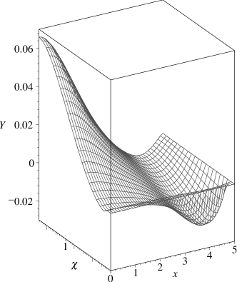
Figure 3: The numerical solution of $Y$ for $(1/L)=0.06$ as a function of $x$ and $\chi$. Here, $x_{\rm out}=5$ and $\Delta x=0.05$ are adopted. The value of $Y$ does not decay properly at the distant region. Besides, there is an unnatural jump in the value of $Y$ between the grids $J=1$ and $2$ (i.e. $\chi=\Delta\chi$ and $2\Delta\chi$).

When both $(1/L)$ and $x_{\rm out}$ are not so large (e.g. $(1/L)=0.02$ and $x_{\rm out}=5.0$), the numerical solutions for $T$, $X$, and $Y$ (apparently) look natural, and their gross features coincide with those of the solution in [29]. For example, the figures in [29] indicate that $Y\geq 0$ and $Y$ takes the maximum value where the brane and the horizon cross each other, and the same feature holds in our numerical data. However, as $(1/L)$ is increased for a fixed $x_{\rm out}$, a strange behavior becomes relevant. Figure 3 shows our numerical solution of $Y(x,\chi)$ for $(1/L)=0.06$, $x_{\rm out}=5.0$, and $\Delta x=0.05$. The value of $Y$ does not decay properly at the distant region. Moreover, there is an unnatural jump in the values of $Y$ at the grids $J=1$ and $2$ (i.e. $\chi=\Delta\chi$ and $2\Delta\chi$). This is in contrast to the case of a zero tension brane in Sec. 4, where the error in $Y$ is suppressed in the neighborhood of the axis. As the characteristic error in $Y$, we define the following quantity:

$$\delta_{Y}:=\max\left|Y(x,2\Delta\chi)-Y_{\rm ext}(x)\right|.$$ (29)

Here, $Y_{\rm ext}(x)$ means the extrapolated value of $Y$ at $\chi=2\Delta\chi$ using the values of $Y(x,0)$ and $Y(x,\Delta\chi)$. Let us observe how the value of $\delta_{Y}$ depends on $x_{\rm out}$ and $(1/L)$.

Figure 4: Dependence of the error $\delta_{Y}$ in $Y$ on the location of the outer boundary $x_{\rm out}$. The left plot shows the cases of $(1/L)=0.005$ ($\circ$), $0.01$ ($\blacktriangledown$), and $0.02$ ($\diamond$) for a fixed resolution $\Delta x=0.05$. The right plot shows the results by the two different resolutions, $\Delta x=0.05$ ($\blacktriangledown$) and $0.025$ ($\triangledown$), in the case $(1/L)=0.01$. In the range $x_{\rm out}\lesssim\log(4L)$, the error value $\delta_{Y}$ does not depend on the resolution and decreases with the increase in $x_{\rm out}$. In the range $x_{\rm out}\gtrsim\log(4L)$, the error value $\delta_{Y}$ depends on the resolution and becomes larger with the increase in $x_{\rm out}$ in both resolutions. The error is interpreted as the boundary error and the nonsystematic error for $x_{\rm out}\lesssim\log(4L)$ and $x_{\rm out}\gtrsim\log(4L)$, respectively. See text for details.

Figure 4 shows the value of $\delta_{Y}$ as a function of $x_{\rm out}$. In the left plot, the cases $(1/L)=0.005$, $0.01$, and $0.02$ are shown for a fixed $\Delta x=0.05$. As $x_{\rm out}$ is increased, $\delta_{Y}$ decreases at first, but later increases. The change from decrease to increase happens at $x_{\rm out}\simeq\log(4L)$ (i.e. $\rho_{\rm out}\simeq 4\ell$). This behavior is opposite to our expectation, since the error has to continue to decrease as $x_{\rm out}$ is increased until it hits one of the relaxation and grid errors which are both $\lesssim 10^{-5}$. Therefore, although the error $\delta_{Y}$ for $x_{\rm out}\lesssim\log(4L)$ can be interpreted as the boundary error, we have detected the nonsystematic error in the range $x_{\rm out}\gtrsim\log(4L)$. The right plot shows the comparison between the two resolutions, $\Delta x=0.05$ and $0.025$, for a fixed $(1/L)=0.01$. For $x_{\rm out}\lesssim\log(4L)$, the two error values almost coincide and they are determined only by $x_{\rm out}$. Therefore, we can confirm that the error in this region is the boundary error. On the other hand, for $x_{\rm out}\lesssim\log(4L)$, the error $\delta_{Y}$ depends on the resolution. However, they are not the grid errors, since the grid errors are $\lesssim 10^{-5}$ and $\sim 10^{-7}$ for $\Delta x=0.05$ and $0.025$, respectively, as proved in Sec. 4. The relaxation error is also $\sim 10^{-6}$. The important feature is that in both resolutions, the errors become larger as $x_{\rm out}$ is increased. Therefore, we again confirm that the error in the range $x_{\rm out}\gtrsim\log(4L)$ is the nonsystematic error.

Figure 5: Dependence of the error $\delta_{Y}$ in $Y$ on the values of $(1/L)$. The left plot shows the cases of $x_{\rm out}=4.0$ ($\times$), $5.0$ ($\vartriangle$), and $6.0$ ($\bullet$) for a fixed resolution $\Delta x=0.05$. The right plot shows the results by the two different resolutions, $\Delta x=0.05$ ($\vartriangle$) and $0.025$ ($\blacktriangle$), in the case $x_{\rm out}=5.0$. The boundary error $\delta_{Y}$ in the range $(1/L)\lesssim 4\exp(-x_{\rm out})$ scarcely depends on the resolution and grows linearly with respect to $(1/L)$. The nonsystematic error in the range $(1/L)\gtrsim 4\exp(-x_{\rm out})$ depends on the resolution and grows nonlinearly with respect to $(1/L)$ in both resolutions.

Figure 5 shows the value of $\delta_{Y}$ as a function of $(1/L)$. The left plot shows the cases of $x_{\rm out}=4.0$, $5.0$, and $6.0$ for a fixed $\Delta x=0.05$. We see the boundary error in the range $(1/L)\lesssim 4\exp(-x_{\rm out})$, and it grows linearly with respect to $(1/L)$ for a fixed $x_{\rm out}$. This is natural because the value of $Y$ itself grows linearly with $(1/L)$. On the other hand, we see the nonsystematic error in the range $(1/L)\gtrsim 4\exp(-x_{\rm out})$. In contrast to the boundary error, the nonsystematic error grows nonlinearly with respect to $(1/L)$ for a fixed $x_{\rm out}$, and the growth rate is roughly given by $\sim(1/L)^{4}$. The right plot shows the comparison between the two different resolutions, $\Delta x=0.05$ and $0.025$, for a fixed $x_{\rm out}=5.0$. Again, we confirm that the boundary errors are almost same for both resolutions, while the nonsystematic error depends on the resolution. Although the nonsystematic error for $\Delta x=0.025$ is smaller than that for $\Delta x=0.05$ if compared with the same $(1/L)$, the nonlinear growth $\sim(1/L)^{4}$ is observed in both resolutions.

5.2 The error in the surface gravity $\kappa$

Figure 6: The same as Fig. 4 but for the error $\delta_{\kappa}$ in the surface gravity. The boundary error and the nonsystematic error can be seen for $x_{\rm out}\lesssim\log(4L)$ and $x_{\rm out}\gtrsim\log(4L)$, respectively, also in the error $\delta_{\kappa}$.

Figure 7: The same as Fig. 5 but for the error $\delta_{\kappa}$ in the surface gravity. The nonlinear growth of the nonsystematic error with respect to $(1/L)$ is seen also for $\delta_{\kappa}$.

As another example of the numerical error, we look at the error in the surface gravity $\kappa$. As mentioned in Sec. 2.2, there are the four boundary conditions on the horizon, and the three of them are chosen in our numerical calculation. Since we omitted the boundary condition that corresponds to the constancy of $\kappa$ on the horizon, we have to check if it is satisfied within the amount of the systematic errors after generating the solutions. In order to evaluate the error in $\kappa$, we define

$$\delta_{\kappa}:=\max[\kappa]-\min[\kappa].$$ (30)

Figure 6 shows the value of $\delta_{\kappa}$ as a function of $x_{\rm out}$. The left plot shows the cases of $(1/L)=0.005$, $0.01$, and $0.02$ for a fixed $\Delta x=0.05$, and the right plot shows the comparison between the two different resolutions, $\Delta x=0.025$ and $0.05$, for a fixed $(1/L)=0.01$. Although $\delta_{\kappa}$ is smaller than $\delta_{Y}$, they have common features. Namely, if $x_{\rm out}$ is increased, the value of $\delta_{\kappa}$ decreases at first but begins to increase at $x_{\rm out}\simeq\log(4L)$. Therefore, also for $\delta_{\kappa}$, we find the boundary error and the nonsystematic error in the ranges $x_{\rm out}\lesssim\log(4L)$ and $x_{\rm out}\gtrsim\log(4L)$, respectively. Although the nonsystematic errors for the resolutions $\Delta x=0.05$ and $0.025$ have a little different values, they both become larger as $x_{\rm out}$ is increased.

Figure 7 shows the value of $\delta_{\kappa}$ as a function of $(1/L)$. The left plot shows the cases of $x_{\rm out}=4.0$, $5.0$, and $6.0$ for a fixed $\Delta x=0.05$, and the right plot shows the comparison between the two different resolutions, $\Delta x=0.05$ and $0.025$, for a fixed $x_{\rm out}=5.0$. The boundary error for $\delta_{\kappa}$ is almost constant when $(1/L)$ is changed and this is different from the behavior of $\delta_{Y}\propto(1/L)$. This is because the surface gravity $\kappa$ itself is almost constant. On the other hand, for a fixed $x_{\rm out}$, the nonsystematic error for $\delta_{\kappa}$ grows nonlinearly with respect to $(1/L)$. Although the nonsystematic error for $\Delta x=0.025$ is smaller than that for $\Delta x=0.05$, we observe the nonlinear growth with respect to $(1/L)$ in both resolutions, and again the growth rate is roughly $\sim(1/L)^{4}$.

5.3 Comparison with the perturbative study

In the next subsection, we discuss the fact that the nonsystematic error has a crucial meaning for the existence of the solution. But in the perturbative level, the (at least $C^{1}$) solution of a black hole on a brane was found for a small mass [30, 31]. In this subsection, let us examine whether our numerical solution is consistent with the perturbative study if the numerical errors are ignored. Since the perturbative study [30, 31] was done in a different gauge condition, the direct comparison between the metric functions is not possible. However, we can compare the two results by calculating nondimensional quantities on the horizon.

Figure 8: The behavior of $\kappa\tilde{\rho}_{\rm b}$ as a function of $(1/L)$. The numerical data for $x_{\rm out}=5.0$ and $\Delta x=0.05$ is shown by squares ($\square$). The prediction by the perturbative study [31] is shown by a solid line. The two results agree well for $(1/L)\ll 1$.

Figure 9: The same as Fig. 8 but for the quantity $\tilde{\rho}_{\rm eff}/\tilde{\rho}_{\rm b}$. Again, the two results agree well for $(1/L)\ll 1$.

As the first example, let us consider the product of the surface gravity $\kappa$ and the proper radius of the horizon on the brane

$$\tilde{\rho}_{\rm b}:=\rho_{h}\exp\left[C(\rho_{h},\pi/2)\right]$$ (31)

(i.e., the proper circumference divided by $2\pi$). Here, $C$ is written as a function of the coordinates $(\rho,\chi)$. Figure 9 shows the relation between $(1/L)$ and $\kappa\tilde{\rho}_{\rm b}$ for fixed values of $\Delta x=0.05$ and $x_{\rm out}=5.0$. The prediction by the perturbative study [31] is shown by a solid line (see Appendix A for a derivation). The two results agree well in the regime $(1/L)\ll 1$.

As another example, let us consider the quantity related to the distortion of the horizon. For this purpose, we define the effective radius of the horizon in the 5-dimensional sense as

$$\tilde{\rho}_{\rm eff}:=\left({A_{5}}/{\Omega_{3}}\right)^{1/3},$$ (32)

and calculate the ratio of the effective radius $\tilde{\rho}_{\rm eff}$ to the proper radius on the brane $\tilde{\rho}_{\rm b}$. Here, $\Omega_{3}$ denotes the 3-dimensional area of a unit sphere, $\Omega_{3}=2\pi^{2}$, and $A_{5}$ is the area of the horizon

$$A_{5}:=2\Omega_{2}\int_{0}^{\pi/2}\left(\frac{\ell}{z}\right)^{3}e^{R+2C}\sin^{2}\chi d\chi,$$ (33)

with $\Omega_{2}:=4\pi$. Figure 9 shows the relation between $(1/L)$ and $\tilde{\rho}_{\rm eff}/\tilde{\rho}_{\rm b}$ for fixed values of $\Delta x=0.05$ and $x_{\rm out}=5.0$. The value of $\tilde{\rho}_{\rm eff}/\tilde{\rho}_{\rm b}$ decreases as $(1/L)$ is increased, and thus the horizon becomes flattened. The prediction by the perturbative study [31] is shown by the solid line (see Appendix A for a derivation), and the numerical data agrees well with the perturbative study in the regime $(1/L)\ll 1$.

As found above, our numerical data is consistent with the perturbative study [30, 31] if the numerical errors are ignored. This result can be interpreted as the evidence for the correctness of our code as well as the correctness of the perturbative study.

5.4 Interpretation

Now, let us discuss the interpretation of our results. In Secs. 5.1 and 5.2, we have found the nonsystematic errors in our numerical data for both the error $\delta_{Y}$ in $Y$ and the error $\delta_{\kappa}$ in the surface gravity. These nonsystematic errors become relevant for $x_{\rm out}\gtrsim\log(4L)$, and grow nonlinearly with respect to $(1/L)$ for a fixed $x_{\rm out}$. On the other hand, as shown in Sec. 5.3, our results are consistent with the perturbative study [30, 31] for a small black hole on a brane in the regime $(1/L)\ll 1$ if the numerical errors are ignored. In order to interpret these strange results, we suggest and discuss the following three possibilities: (I) The numerical code is wrong; (II) The solution does not exist; and (III) The solution exists but it is numerically unstable.

We understand that the possibility (I) is the case that most readers might expect. However, we have successfully reproduced the Schwarzschild solution for $(1/L)=0$ in Sec. 4. Moreover, our results for $(1/L)\ll 1$ are consistent with the perturbative study [30, 31]. This guarantees that at least the linear terms in $\rho/\ell$ are correctly included in our code. Therefore, our task is to properly include the other nonlinear terms, and this can be done by careful checks. For this reason, we definitely exclude the possibility (I).

We turn to the possibility (II) that no solution exists. Here, we consider the case that no regular solution exists but the solution to the finite difference equations exist. Since such a case can happen, it is generally warned that at least the appropriate convergence has to be checked in numerical calculations. Let us recall Figs. 4, 5, 6, and 7. In the right plots of those figures, we compared the errors of the results by the two different resolutions, $\Delta x=0.05$ and $0.025$, and found that the numerical data does not show the appropriate convergence. If we assume that the solution to the finite difference equations is unique (see possibility (III) for the meaning of this assumption), this indicates that a regular solution does not exist at least for finite $x_{\rm out}$. If the error continued to decrease with the increase in $x_{\rm out}$, the solution would exist for $x_{\rm out}=\infty$. However, the fact is that the error becomes larger with the increase in $x_{\rm out}$ in the range $x_{\rm out}\gtrsim\log(4L)$, raising doubts for the existence of the solution also for $x_{\rm out}=\infty$.

For small $(1/L)$, the solution exists at the perturbative level [31] and our numerical data is consistent with this study. But we also found the nonsystematic error that grows nonlinearly with respect to $(1/L)$. Here, let us recall the fact that the regularity of the horizon is not perfectly guaranteed in the perturbative study [31] (see also Appendix A). If the perturbation becomes singular at the higher-order perturbation, what happens in the numerical calculation? Such a singular effect should appear as the numerical error that behaves in a nonsystematic way. The nonlinear growth of the nonsystematic error with respect to $(1/L)$ supports this view. We consider that this is the most natural interpretation of our result. If this is the case, the regular solution does not exist at least to this setup.

It is interesting to ask at which order the perturbation becomes singular. This is a difficult question to answer, and we just make a speculation here. In Figs. 5 and 7, we found that the nonsystematic error grows quite rapidly, $\sim(1/L)^{4}$, as $(1/L)$ is increased. If we assume that this power of the nonsystematic error reflects the order at which the perturbation becomes singular, the singular behavior might appear at the 4th-order perturbation.

Readers might wonder why we do not claim the existence of the solution at least for the range $(1/L)\ll 1$ in spite of the consistency of our numerical data with the perturbative study and the small values of the nonsystematic error. In fact, we have reproduced the results of the perturbative study for $(1/L)\ll 1$ with a typical numerical error $\lesssim 0.1\%$. However, the merits in the numerical calculation is the ability to explore the nonlinear regime in $(1/L)$, and our results obviously show that something is wrong at the nonlinear level. In such a situation, it is much more dangerous to claim the existence of the solution however small the detected error is. We consider that this is a common sense for numerical researchers who are serious in analyzing the numerical errors.

Readers might also expect that the solution exists for small $(1/L)$ and it vanishes at some critical point as $(1/L)$ is increased, as suggested in Ref. [17]. We do not consider that this is the case, because as shown in Figs. 4 and 6, the nonsystematic error becomes relevant for $x_{\rm out}\gtrsim\log(4L)$ for very small $(1/L)$ values such as $(1/L)=0.005$. To support this view, let us look at the existing example by the author and his collaborator [36] where disappearance of a solution was actually observed. In that paper, we numerically studied the apparent horizon formation in high-energy particle collisions, and found that the solution of the apparent horizon exists for a small impact parameter $b$, but it disappears at the maximal impact parameter $b_{\rm max}$. As shown in Fig. 2 of Ref. [36], there is a clear signal of $b_{\rm max}$ such that $dr_{\rm min}/db$ diverges. Although the numerical error grows as $b$ is increased, the error turns out to be the grid error whose growth is driven by the distortion of the apparent horizon. This is the typical phenomena that happens when a solution vanishes as the system parameter is changed. However, in the present setup, we do not find any signal of disappearance of the solution. Besides, the numerical error that grows with $(1/L)$ is not the grid error, but has turned out to be the nonsystematic error. These features are all in contrast to the case of [36].

Finally, let us discuss the third possibility (III) that the solution exists but it is numerically unstable. Here, we refer to the case that a regular solution exists and that two or more solutions to the finite difference equations exist. Among these numerical solutions, only one solution approximates the regular solution, and our obtained solution is one of the other artificial solutions that do not represent the true solution. We consider that this case is unlikely, since our solution reproduces the result of the perturbative study for $(1/L)\ll 1$ and hence it does not seem to be artificial. However, at the same time, we cannot rigorously show the uniqueness of the solution to the finite difference equations since they are highly complicated. As a result, we cannot rigorously claim the nonexistence of the solution, i.e., that the possibility (II) is the case. For this reason, our results also have to be carefully interpreted as well as the other numerical or perturbative studies. In order to show the nonexistence of solutions rigorously, a proof by the method of the mathematical relativity will be required.

6 Summary and discussion

In this paper, we studied a black hole on a brane in the RS II scenario using the numerical code having almost 4th-order accuracy. Although we successfully reproduced the Schwarzschild solution in the case of a zero tension brane (Sec. 4), the nonsystematic error was detected for the cases of a nonzero tension brane (Secs. 5.1 and 5.2). This nonsystematic error becomes relevant for $x_{\rm out}\gtrsim\log(4L)$ even for a very small $(1/L)$, and it grows nonlinearly with respect to $(1/L)$ for a fixed $x_{\rm out}$. On the other hand, our numerical data agrees very well with the perturbative study [30, 31] if the numerical error is ignored (Sec. 5.3). In Sec. 5.4, we discussed the interpretation of our result. The most natural interpretation is that the perturbation becomes singular at the higher order in $(1/L)$, and this effect appears as the nonsystematic error in the numerical data [the possibility (II)]. If this is the case, no solution of a black hole on a brane exists. We also pointed out the remaining possibility that the solution exists [the possibility (III)], although it is unlikely. To summarize, our numerical results raise strong doubts for the existence of a static black hole on a brane. To be precise, our claim is: A solution sequence of a static black hole on an asymptotically flat brane that is reduced to the Schwarzschild black hole in the zero tension limit is unlikely to exist. It is also worth pointing out that a similar claim has been made in the context of the AdS/CFT correspondence [14].

In this paper, we focused our attention to the numerical calculations. So far, we have not succeeded in proving the nonexistence of solutions by an analytic method. But, here, we would like to give an analytic discussion that supports it. Let us ask in this way: Suppose the functions $T$, $R$, and $C$ satisfy Eqs (5)–(7) and (9) and the boundary conditions at infinity (11), at the symmetry axis (15)–(14), on the horizon (16)–(19), and ${T_{,\chi}}/{T}=R_{,\chi}=({\rho}/{\ell})(e^{R}-1)$ on the brane. Then, can the function $C$ satisfy the boundary condition $C_{,\chi}=({\rho}/{\ell})(e^{R}-1)$ on the brane? To answer this question, we calculate the difference of the equations (7) and (9). The result is the equation of the form

$$-\rho^{2}C_{,\chi\chi}+C_{,\rho\rho}+F[T_{,\chi\chi},T_{,\chi},R_{,\chi},C_{,\chi},T_{,\rho},R_{,\rho},C_{,\rho},T,R,C,\rho,\chi]=0.$$ (34)

Here, there is no singularity in this equation at $\chi=0$. This is a wave equation where $\chi$ is the “time” coordinate. The “initial condition” is given by $C=R$ and $C_{,\chi}=0$ at $\chi=0$. For given $T$ and $R$, we can “evolve” $C$ using this equation from $\chi=0$ to $\pi/2$. Then, the value of $C_{,\chi}$ at $\chi=\pi/2$ is determined as a result of the “temporal evolution”, and therefore, there is no guarantee that $C$ satisfies the junction condition on the brane $C_{,\chi}=({\rho}/{\ell})(e^{R}-1)$. Although this condition can be satisfied in a special situation (e.g. the spherically symmetric case), such a chance cannot be expected in general. We consider that this discussion is consistent with our numerical results. In Fig. 3, we found an unnatural jump in the value of $Y$ in the neighborhood of the symmetry axis. This would be because the boundary conditions on the brane and at the symmetry axis are incompatible.

Suppose solutions of a static black hole on a brane do not exist in the RS scenarios as discussed in this paper. Then, what happens after the gravitational collapse? As an example, let us consider a head-on collision of high-energy particles. Because of the nonexistence of the solution, one might expect that the black hole does not form in the collision. However, we do not consider that this is the case, since there exist studies on the apparent horizon formation in the RS II scenario [37, 38], and even the formation of a very large apparent horizon is reported [38]. For this reason, the black hole should form. Although the produced black hole relaxes to a quasi-equilibrium state by emitting the gravitational radiation, it does not completely become static and cannot remain on the brane. In this sense, the black hole is unstable. We suggest two possibilities of the consequences of the instability: the event horizon pinch and the brane pinch.

In the first possibility of the event horizon pinch, we refer to the case where the brane scarcely moves and the cross section of the event horizon and the brane shrinks. In the classical general relativity, the pinch of an event horizon is forbidden (e.g. [35]). However, if the radius of the cross section becomes order of the Planck length, the event horizon pinch could happen by quantum gravity effects and the black hole may leave the brane. We consider that this scenario may happen when the horizon radius is sufficiently larger than the bulk curvature scale, since the brane is expected to be rigid in this case.

In the second possibility of the brane pinch, we refer to the case where the event horizon scarcely moves while the brane moves. The motion of the brane continues until it pinches and generates a baby brane. We consider that this scenario may happen when the horizon radius is smaller than the bulk curvature scale, since in this case the brane can easily fluctuate. Basically, this scenario was already suggested and studied in detail in [39, 40, 41, 42] by numerical simulations for a zero tension brane and a more detailed model of a brane (but without the self-gravity effects). In those studies, the authors gave the brane an initial velocity in the bulk direction, and observed the brane pinch. The new insight from the results in the present paper is that such a brane pinch might happen because of the instability without the initial velocity in the bulk direction. We are also able to estimate the time scale of this phenomena. In our numerical data, the nonsystematic error has the order of $\sim(1/L)^{4}$. Since this error amount is expected to cause the temporal evolution, the typical time scale would be $\sim\ell^{4}/\rho_{h}^{3}$. Therefore, the brane pinch may happen relatively slowly unless the velocity in the bulk direction is given. In order to clarify if this is the case, a simulation taking account of the self-gravity effects of the brane is necessary. It also has to be checked if the brane pinch can happen when the $\mathbb{Z}_{2}$-symmetry is imposed.

The above discussion has the following implication for the black hole production at the LHC. If the extra dimension is warped, the produced black hole may escape into the bulk. If this is the case, it is difficult to observe the signals of the Hawking radiation especially from black holes with large mass, since the time scale of the instability may be shorter than the time scale of the evaporation. Therefore, the instability of black holes on a brane gives us many interesting and important issues to be explored.

Appendix A A brief review of the perturbative study

Karasik et al. [30, 31] solved the static solution of a black hole on a brane in the RS scenarios in the case of a small mass by a perturbative study. Here, we summarize the part of their results that is directly related to the discussions in this paper. In this section, we follow their notation. Since they were mainly motivated by the TeV gravity scenarios, they studied in the framework of the RS I scenario. However, their results can be applied also to the RS II scenario by changing the sign of $\ell$.

They considered the situation where the radius of the black hole $\mu:=\sqrt{8G_{5}M/3\pi}$ is much smaller than the bulk curvature scale $\ell$, and adopted the so-called matching method. In this method, the spacetime is a perturbed Schwarzschild black hole in the neighborhood of the horizon and is a perturbed AdS spacetime at the distant region, where $\epsilon:=\mu/\ell$ is the small parameter. In the matching region $\mu\ll r\ll l$, the two approximations both hold and the two solutions can be matched to each other.

In the neighborhood of the horizon, the metric is assumed to be

$$ds^{2}=\left(\frac{\ell}{z}\right)^{2}\left[-Bdt^{2}+\frac{A}{B}d\rho^{2}+2Vd\rho d\psi+\rho^{2}Ud\psi^{2}+\rho^{2}\sin^{2}\psi d\Omega_{2}^{2}\right],$$ (35)

where $z:=\ell-\rho\cos\psi$ and $A$, $B$, $V$, $U$ are the functions of $\rho$ and $\psi$. The background solution is the Schwarzschild solution $A_{0}=U_{0}=1$, $B_{0}=1-1/\rho^{2}$, and $V_{0}=0$. The first order quantities for these functions are given as $\epsilon A_{1}$, $-\epsilon B_{1}$, $\epsilon U_{1}$ and $\epsilon V_{1}$, respectively, and it turns out that they are expressed in terms of $F$, $H$, $F_{,\rho}$, $H_{,\rho}$, $F_{,\psi}$ and $H_{,\psi}$, where $F$ is a gauge function and $H$ is a wave function. The wave function $H$ satisfies the equation

$$(\rho^{2}-1)\left(H_{,\rho\rho}-\frac{H_{,\rho}}{\rho}\right)+H_{,\psi\psi}+2\frac{\cos^{2}\psi+1}{\sin\psi\cos\psi}H_{,\psi}=0.$$ (36)

It was found that when the perturbed AdS metric at the distant region includes only integer powers of $M$, the matched solution in the neighborhood of the horizon is singular at $\rho=1$. However, if we allow the terms with half integer powers of $M$ at the distant region, the metric becomes at least $C^{1}$ and the zeroth and first law of the black hole thermodynamics can be satisfied. The solution of $H$ is

$$H=\delta_{0}-\frac{2}{3\pi}\tilde{Q}_{-1/2}(\rho)g^{(1)}(\psi)+\tilde{Q}_{1/2}(\rho)\left(-\frac{1}{3\pi}g^{(2)}(\psi)+\frac{d_{2}}{\sin^{3}\psi}-\frac{\pi}{3}g^{(3)}(\psi)\right)\\ +\frac{\pi}{3}\left(\tilde{P}_{1/2}(\rho)+\frac{2}{\pi^{2}}\left.\frac{\partial\tilde{Q}_{n-1/2}}{\partial n}\right|_{n=1}\right)g^{(2)}(\psi)+\sum_{\lambda=3}^{\infty}a(\lambda)\tilde{Q}_{(\lambda-1)/2}(\rho)G(\lambda,\psi).$$ (37)

Here, $\tilde{P}_{\nu}:=\rho\sqrt{\rho^{2}-1}P^{1}_{\nu}(2\rho^{2}-1)$, and $\tilde{Q}_{\nu}:=\rho\sqrt{\rho^{2}-1}Q^{1}_{\nu}(2\rho^{2}-1)$, and $g^{(1)}$, $g^{(2)}$, $g^{(3)}$ and $G(\lambda,\psi)$ are some elementary functions of $\psi$ (see Eq. (36) in [31] for details). The values of $\delta_{0}$, $d_{2}$, and $a(\lambda)$ are fixed as $\delta_{0}=d_{2}=0$ and $a(\lambda)=-(16/3\pi)(-1)^{\lambda}/(\lambda^{2}-4)$ by imposing boundary conditions and the zeroth and first laws of the black hole thermodynamics. The expansion of the function $\tilde{Q}_{\nu}$ has the terms proportional to $(\rho^{2}-1)^{n}\log(\rho^{2}-1)$ for integer $n\geq 1$. Hence, $H_{,\rho}$ has the form

$$H_{,\rho}\simeq\frac{h_{0}(\psi)}{\sin^{3}\psi}\left[\log(\rho^{2}-1)+2\gamma_{E}+2\bar{\psi}(1/2)\right]+h_{1}(\psi),$$ (38)

in the neighborhood of the horizon, where $h_{0}(\psi)$ and $h_{1}(\psi)$ are given by Eqs. (44) and (45) in Ref. [31]. Here, a miraculous cancellation happens and $h_{0}(\psi)$ becomes zero. This means that the term proportional to $(\rho^{2}-1)\log(\rho^{2}-1)$ is not included in $H$. Then, the equation (36) implies that $H_{,\rho\rho}$ is also finite. As a result, the function $H$ includes terms proportional to $(\rho^{2}-1)^{n}\log(\rho^{2}-1)$ only for $n\geq 3$.

When the horizon is regular, the location of the horizon $\rho_{H}$ and the surface gravity $\kappa$ are given by

$$\rho_{H}=1+\epsilon\left[-6H(1,\pi/2)+H_{,\rho}(1,\pi/2)\right];$$ (39)

$$\kappa=1+6\epsilon H(1,\pi/2),$$ (40)

from Eqs. (23c) and (23d) in [31], and the 3-dimensional area of the horizon is given by

$$\frac{A_{H}}{A_{H}^{(0)}}=1-\frac{9}{2}\epsilon H(1,\pi/2)$$ (41)

from Eqs. (27) and (30) in [31], where $A_{H}^{(0)}:=2\pi^{2}\mu^{3}$. From these formulas, we immediately find that the product of the surface gravity and the proper radius of the horizon on the brane is $\kappa\rho_{H}=1+\epsilon h_{1}(\pi/2)$. On the other hand, the ratio of the effective horizon radius to the radius on the brane becomes $(A_{H}/A_{H}^{(0)})^{1/3}/\rho_{H}=1+\epsilon\left[(9/2)H(1,\pi/2)-h_{1}(\pi/2)\right]$. Here, $H(1,\pi/2)=8/9\pi$ from Eq. (38) in [31] and $h_{1}(\pi/2)$ is numerically evaluated to be $\simeq 1.087336$. In order to apply to the RS II scenario, we change the sign of $\ell$ and find

$$\kappa\rho_{H}\simeq 1-2.17467\times\frac{\sqrt{2G_{5}M/3\pi}}{\ell};$$ (42)

$$\frac{(A_{H}/A_{H}^{(0)})^{1/3}}{\rho_{H}}\simeq 1-0.371801\times\frac{\sqrt{2G_{5}M/3\pi}}{\ell}.$$ (43)

These formulas are used in Figs. 9 and 9, respectively.

We comment on the remaining issues in this study. In order to guarantee the regularity on the horizon, the Kretchmann scalar $K:=R_{\mu\nu\rho\sigma}R^{\mu\nu\rho\sigma}=K^{(0)}+\epsilon K^{(1)}+\epsilon^{2}K^{(2)}+\cdots$ has to be finite on the horizon. If the function $H$ includes a term proportional to $(\rho^{2}-1)^{3}\log(\rho^{2}-1)$, the third derivative $H_{,\rho\rho\rho}$ logarithmically diverges at $\rho=1$. Although the authors of Ref. [31] have confirmed the absence of the term $H_{,\rho\rho\rho}$ in $K^{(1)}$, there remains a possibility that $K^{(2)}$ diverges. In order to check this, two things are required. First, one needs to confirm if $H_{,\rho\rho\rho}$ really possesses such a logarithmic term. But this is difficult because the coefficient of $(\rho^{2}-1)^{3}\log(\rho^{2}-1)$ in Eq. (37) has the infinite summation of terms whose absolute values become unboundedly large as $\lambda$ is increased. It turns out that this infinite summation does not converge even in the sense of distribution. Therefore, there is an ambiguity in the interpretation of Eq. (37). In the particle physics, several procedures to regularize diverging infinite summations are known. Although it may be possible to regularize the infinite summation in $H$ in a similar way, this is not an easy task, and this situation makes it difficult to confirm the (non)existence of the term proportional to $(\rho^{2}-1)^{3}\log(\rho^{2}-1)$ even numerically. Next, the presence of a logarithmic term in $H_{,\rho\rho\rho}$ does not immediately imply the divergence of the Kretchmann scalar $K$, since the terms from the 2nd-order perturbations may cancel this term. However, the study of the 2nd-order perturbation is also a difficult task.

Finally, even if the regularity of the perturbation is established to some order, there remains the possibility that the metric becomes singular at the next order. If our interpretation in Sec. 5.4 is correct, the singular behavior might appear at the 4th-order perturbation. Therefore, it may be very difficult to check the (non)existence of solutions of a black hole on a brane by the perturbative method.

References

- [1] L. Randall and R. Sundrum, A large mass hierarchy from a small extra dimension, Phys. Rev. Lett. 83 (1999) 3370 [hep-ph/9905221].
- [2] L. Randall and R. Sundrum, An alternative to compactification, Phys. Rev. Lett. 83 (1999) 4690 [hep-th/9906064].
- [3] T. Banks and W. Fischler, A model for high energy scattering in quantum gravity, hep-th/9906038.
- [4] S. Dimopoulos and G. Landsberg, Black holes at the LHC, Phys. Rev. Lett. 87 (2001) 161602 [hep-ph/0106295].
- [5] S. B. Giddings and S. Thomas, High energy colliders as black hole factories: The end of short distance physics, Phys. Rev. D 65 (2002) 056010 [hep-ph/0106219].
- [6] J. Garriga and T. Tanaka, Gravity in the brane-world, Phys. Rev. Lett. 84 (2000) 2778 [hep-th/9911055].
- [7] S. B. Giddings, E. Katz and L. Randall, Linearized gravity in brane backgrounds, J. High Energy Phys. 03 (2000) 023 [hep-th/0002091].
- [8] S. W. Hawking, T. Hertog and H. S. Reall, Brane new world, Phys. Rev. D 62 (2000) 043501 [hep-th/0003052].
- [9] M. J. Duff and J. T. Liu, Complementarity of the Maldacena and Randall-Sundrum pictures, Class. and Quant. Grav. 18 (2001) 3207 [Phys. Rev. Lett. 85 (2000) 2052] [hep-th/0003237].
- [10] T. Shiromizu and D. Ida, Anti-de Sitter no hair, AdS/CFT and the brane-world, Phys. Rev. D 64 (2001) 044015 [hep-th/0102035].
- [11] T. Tanaka, Classical black hole evaporation in Randall-Sundrum infinite braneworld, Prog. Theor. Phys. Suppl. 148 (2003) 307 [gr-qc/0203082].
- [12] R. Emparan, A. Fabbri and N. Kaloper, Quantum black holes as holograms in AdS braneworlds, J. High Energy Phys. 08 (2002) 043 [hep-th/0206155].
- [13] P. R. Anderson, R. Balbinot and A. Fabbri, Cutoff AdS/CFT duality and the quest for braneworld black holes, Phys. Rev. Lett. 94 (2005) 061301 [hep-th/0410034].
- [14] A. Fabbri, S. Farese, J. Navarro-Salas, G. J. Olmo and H. Sanchis-Alepuz, Semiclassical zero-temperature corrections to Schwarzschild spacetime and holography, Phys. Rev. D 73 (2006) 104023 [hep-th/0512167].
- [15] A. L. Fitzpatrick, L. Randall and T. Wiseman, On the existence and dynamics of braneworld black holes, J. High Energy Phys. 11 (2006) 033 [hep-th/0608208].
- [16] A. Fabbri and G. P. Procopio, Quantum Effects in Black Holes from the Schwarzschild Black String?, Class. and Quant. Grav. 24 (2007) 5371 [\arXivid0704.3728].
- [17] T. Tanaka, Implication of Classical Black Hole Evaporation Conjecture to Floating Black Holes, \arXivid0709.3674.
- [18] R. Gregory, S. F. Ross and R. Zegers, Classical and quantum gravity of brane black holes, J. High Energy Phys. 09 (2008) 029 [\arXivid0802.2037].
- [19] R. Emparan, G. T. Horowitz and R. C. Myers, Exact description of black holes on branes, J. High Energy Phys. 01 (2000) 007 [hep-th/9911043].
- [20] R. Emparan, G. T. Horowitz and R. C. Myers, Exact description of black holes on branes. II: Comparison with BTZ black holes and black strings, J. High Energy Phys. 01 (2000) 021 [hep-th/9912135].
- [21] J. F. Plebanski and M. Demianski, Rotating, charged, and uniformly accelerating mass in general relativity, Ann. Phys. (NY) 98 (1976) 98.
- [22] N. Dadhich, R. Maartens, P. Papadopoulos and V. Rezania, Black holes on the brane, Phys. Lett. B 487 (2000) 1 [hep-th/0003061].
- [23] A. Chamblin, H. S. Reall, H. a. Shinkai and T. Shiromizu, Charged brane-world black holes, Phys. Rev. D 63 (2001) 064015 [hep-th/0008177].
- [24] P. Kanti and K. Tamvakis, Quest for localized 4-D black holes in brane worlds, Phys. Rev. D 65 (2002) 084010 [hep-th/0110298].
- [25] P. Kanti, I. Olasagasti and K. Tamvakis, Quest for localized 4-D black holes in brane worlds. II: Removing the bulk singularities, Phys. Rev. D 68 (2003) 124001 [hep-th/0307201].
- [26] R. Casadio, A. Fabbri and L. Mazzacurati, New black holes in the brane-world?, Phys. Rev. D 65 (2002) 084040 [gr-qc/0111072].
- [27] R. Casadio and L. Mazzacurati, Bulk shape of brane-world black holes, Mod. Phys. Lett. A 18 (2003) 651 [gr-qc/0205129].
- [28] C. Charmousis and R. Gregory, Axisymmetric metrics in arbitrary dimensions, Class. and Quant. Grav. 21 (2004) 527 [gr-qc/0306069].
- [29] H. Kudoh, T. Tanaka and T. Nakamura, Small localized black holes in braneworld: Formulation and numerical method, Phys. Rev. D 68 (2003) 024035 [gr-qc/0301089].
- [30] D. Karasik, C. Sahabandu, P. Suranyi and L. C. R. Wijewardhana, Small (1-TeV) black holes in Randall-Sundrum I scenario, Phys. Rev. D 69 (2004) 064022 [gr-qc/0309076].
- [31] D. Karasik, C. Sahabandu, P. Suranyi and L. C. R. Wijewardhana, Small black holes on branes: Is the horizon regular or singular?, Phys. Rev. D 70 (2004) 064007 [gr-qc/0404015].
- [32] H. Kodama, Accelerating a Black Hole in Higher Dimensions, Prog. Theor. Phys. 120 (2008) 371 [\arXivid0804.3839].
- [33] H. Kodama and A. Ishibashi, A master equation for gravitational perturbations of maximally symmetric black holes in higher dimensions, Prog. Theor. Phys. 110 (2003) 701 [hep-th/0305147].
- [34] A. Ishibashi and H. Kodama, Stability of higher-dimensional Schwarzschild black holes, Prog. Theor. Phys. 110 (2003) 901 [hep-th/0305185].
- [35] R. Wald, General Relativity (University of Chicago Press, Chicago, 1984).
- [36] H. Yoshino and Y. Nambu, Black hole formation in the grazing collision of high-energy particles, Phys. Rev. D 67 (2003) 024009 [gr-qc/0209003].
- [37] T. Shiromizu and M. Shibata, Black holes in the brane world: Time symmetric initial data, Phys. Rev. D 62 (2000) 127502 [hep-th/0007203].
- [38] N. Tanahashi and T. Tanaka, Time-symmetric initial data of large brane-localized black hole in RS-II model, J. High Energy Phys. 03 (2008) 041 [\arXivid0712.3799].
- [39] A. Flachi and T. Tanaka, Escape of black holes from the brane, Phys. Rev. Lett. 95 (2005) 161302 [hep-th/0506145].
- [40] A. Flachi, O. Pujolas, M. Sasaki and T. Tanaka, Black holes escaping from domain walls, Phys. Rev. D 73 (2006) 125017.
- [41] A. Flachi, O. Pujolas, M. Sasaki and T. Tanaka, Critical escape velocity of black holes from branes, Phys. Rev. D 74 (2006) 045013 [hep-th/0604139].
- [42] A. Flachi and T. Tanaka, Branes and black holes in collision, Phys. Rev. D 76 (2007) 025007 [hep-th/0703019].