A bijectional attack on the Razumov-Stroganov conjecture

Abstract

We attempt to prove the Razumov-Stroganov conjecture using a bijectional approach. We have been unsuccessful but we believe the techniques we present can be used to prove the conjecture.

1 Introduction

Ever since the discovery of alternating sign matrices (ASM), the conjecture on the number of such matrices [1] and the proof of this conjecture in [2] (followed by a shorter proof in [3]), a number of interesting structures have been found which are counted by the ASM numbers [4]. One of these structures is that of fully packed loops which has given rise to another beautiful conjecture, formulated in [5, 6], and now popularly known as the Razumov-Stroganov conjecture.

This conjecture, motivated by some exactly solvable models in statistical physics, is about seven years old and already several connections have been found to other combinatorial objects. The literature on this subject is already very large and we will not be able to survey the complete literature. Readers are referred to the papers [7, 8, 9] for more references.

The proof has been found only in some restricted cases [9]. This has also motivated a bunch of refined conjectures, starting with [8]. All of these proofs and refined conjectures generally involve connections to other combinatorial objects and might be a red herring. In this short letter, we suggest a completely self-contained approach which is more combinatorial. This might lead to a proof of the Razumov-Stroganov conjecture.

The paper is organized as follows. In Section 2, we give the basic definitions and set the notation. In Section 3, we restate the conjecture combinatorially, and in Section 4, we propose a mechanism for tackling this restatement. Lastly, in Section 5, we mention some computer experiments which have been successful for smaller sizes but have not yielded the proposed bijection.

2 Definitions

Fully Packed Loops (FPLs) of size $n$ are configurations of lattice paths which are drawn in a square lattice of dimensions $n\times n$ as follows. One assigns the labels $1,\dots,2n$ on the $4n$ endpoints of the lattice alternatively. Subsequently, one connects the endpoint labels pairwise via paths on the lattice so that there are no crossings. Note that one is allowed to fill in loops also. The important point is that these lattice paths have to cover the entire square lattice. It turns out that FPLs are in bijection with Alternating Sign Matrices (ASMs) and therefore the number of FPLs is given by the ASM numbers $A_{n}$ [2, 3],

$$A_{n}=\prod_{i=0}^{n-1}\frac{(3i+1)!}{(n+i)!}.$$ (2.1)

Let us denote the set of FPLs of size $n$ as $F_{n}$. The number of ways of connecting $2n$ endpoints on a circle is the Catalan number $C_{n}$. We can count the number of FPLs according to the connectivity of its endpoints. Let the connectivities be labelled $\pi_{j}$, $j=1,\dots,C_{n}$. Then we let $A(\pi_{j})$ be the number of FPLs with connectivity $\pi_{j}$.

On the set of endpoints, one can define the operators $e_{i}$ for $i\in[1,2n]$ in the following way. Suppose in a particular connectivity $\pi$, $i$ joins $j$ and $i+1$ joins $k$. Then $e_{i}(\pi)$ is the new connectivity obtained by connecting $i$ to $i+1$ (cyclically) and $j$ to $k$. It is easy to see that this is a valid connectivity also. These $e_{i}$ satisfy the defining relations of the Temperley-Lieb algebra,

$$\begin{split}e_{i}^{2}&=e_{i},\\ [e_{i},e_{j}]&=0,\qquad\text{for }|i-j|\geq 2,\\ e_{i}e_{i\pm 1}e_{i}&=e_{i}.\end{split}$$ (2.2)

Consider the vector space whose basis consists of all connectivities $\pi_{j}$, $j=1,\dots,C_{n}$. Since the operators $e_{i}$, $i=1,\dots,2n$ act on connectivities, one can construct a matrix for each $e_{i}$ in that basis. Since every $e_{i}$ takes any basis vector to another single basis vector, the matrix must have a single one in every column, the rest being zeros. This ensures that the vector $w=(1,\dots,1)$ satisfies $we_{i}=w$ for all $i$. Since $e_{i}$ is a nonnegative integer matrix, it has a largest eigenvalue by the Perron-Frobenius theorem, the corresponding eigenvector being positive. Thus, $w$ is the left Perron-Frobenius eigenvector for each $e_{i}$.

Define the “Hamiltonian” matrix,

$$H=\sum_{i=1}^{2n}e_{i}.$$ (2.3)

$w$ is also the left eigenvector of $H$ with the largest eigenvalue $2n$. Obviously, $H$ also has a single right eigenvector with the same eigenvalue. Call it $\Psi$. We can choose $\Psi$ to have positive integer entries, and can expand it in our original basis. Then the Razumov-Stroganov conjecture states that

$$\Psi=\sum_{j=1}^{C_{n}}A(\pi_{j})\pi_{j}.$$ (2.4)

3 A Combinatorial Restatement of the Conjecture

To restate the conjecture we rewrite $H\Psi$,

$$\begin{split}\left(\sum_{i=1}^{2n}e_{i}\right)\left(\sum_{j=1}^{C_{n}}A(\pi_{j})\pi_{j}\right)&=\sum_{j=1}^{C_{n}}A(\pi_{j})\left(\sum_{i=1}^{2n}e_{i}\pi_{j}\right),\\ &=\sum_{j=1}^{C_{n}}A(\pi_{j})\left(\sum_{\begin{subarray}{c}i=1,k=1\\ e_{i}\pi_{j}=\pi_{k}\end{subarray}}^{2n,C_{n}}\pi_{k}\right),\\ &=\sum_{k=1}^{C_{n}}\pi_{k}\left(\sum_{\begin{subarray}{c}i=1,j=1\\ e_{i}\pi_{j}=\pi_{k}\end{subarray}}^{2n,C_{n}}A(\pi_{j})\right).\end{split}$$ (3.1)

Since $H\Psi=2n\Psi$ and the $\pi_{k}$’s are independent vectors, we must have

$$\sum_{\begin{subarray}{c}i=1,j=1\\ e_{i}\pi_{j}=\pi_{k}\end{subarray}}^{2n,C_{n}}A(\pi_{j})=2nA(\pi_{k}),\qquad\text{for all }k=1,\dots,C_{n}.$$ (3.2)

This restatement has the advantage that it involves only the number of FPLs for a given connectivity and in that sense, is more combinatorial. There is no mention of any matrices, eigenvalues and algebras. To the best of our knowledge, this is the first time the Razumov-Stroganov conjecture has been interpreted this way.

We comment that another way to think of (3.2) is that the map $\pi\to A(\pi)$ is a “harmonic function” on the graph of connectivities, where $\pi$ has the $2n$ neighbors $e_{i}\pi$ ($i=1,\dots,2n$).

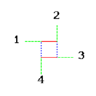
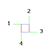
Figure 1: The two FPLs for $n=2$. The red lines represent the paths.

Let us consider a simple example. When $n=2$, we have two connectivities on four points, $\pi_{1}=(12)(34),\,\pi_{2}=(14)(23)$ with $A(\pi_{1})=A(\pi_{2})=1$. These FPLs are shown in Figure 1. The operators $e_{i}$ act in a straightforward manner:

$$\begin{split}e_{1}(\pi_{1})=e_{1}(\pi_{2})=e_{3}(\pi_{1})=e_{3}(\pi_{2})=\pi_{1},\\ e_{2}(\pi_{1})=e_{2}(\pi_{2})=e_{4}(\pi_{1})=e_{4}(\pi_{2})=\pi_{1}.\end{split}$$ (3.3)

For $k=1$, the left hand side is $2A(\pi_{1})+2A(\pi_{2})$ (when $i=1,3$), which is also equal to the right hand side, $4A(\pi_{1})$. Similarly for $k=2$.

(3.2) can be interpreted as a statement of the equality of the cardinality of two sets in the following way. Let

$$\begin{split}{\mathcal{A}}_{k}&=\{(i,f)|i\in[1,2n],f\in F_{n},\pi(f)=\pi_{k}\},\\ {\mathcal{B}}_{k}&=\{(j,g)|j\in[1,2n],g\in F_{n},e_{j}(\pi(g))=\pi_{k}\},\end{split}$$ (3.4)

be two subsets of the product set $[1,2n]\times F$. Then the restatement (3.2) is equivalent to the statement

$$|{\mathcal{A}}_{k}|=|{\mathcal{B}}_{k}|\qquad\text{for all }k=1,\dots,C_{n}.$$ (3.5)

4 Alternating Paths

The equation (3.5) is a conjectured equinumeracy where the index varies among all link patterns. We conjecture that something stronger is true. Namely, a bijection in which the index varies among all FPLs. We suggest that is possible, given an FPL $f$ of size $n$ and an integer $i$ between $1$ and $2n$, to choose in an invertible way another FPL $g$ and another integer $j$ between $1$ and $2n$ so that $e_{i}(\pi(g))=\pi(f)$. The role of $j$ would be to provide the inversion. We give in this section such a procedure, which if used correctly, would yield precisely the correct bijection. The main idea is that of alternating paths.

Recall that the FPL of size $n$ can be represented as a subset of the edges of the two dimensional square lattice whose vertex coordinates lie between $1$ and $n$ plus some additional edges needed to describe the alternating boundaries. For the purposes of defining alternating paths we do not need the additional boundary edges. Let us define the set of all possible edges:

$$S=\{[(i,j),(i+1,j)],[(i,j),(i,j+1)]|\,i,j\in(1,n-1)\},$$

which has cardinality $2n(n-1)$. The FPL is then simply defined by a set of edges $E\subset S$ which has cardinality $n(n-1)$. Then one can define the converse FPL by the set $\bar{E}=S\setminus E$ and of course $\bar{\bar{E}}=E$. In Figure 1, the blue lines represent the interior part of the converse FPL.

We define an alternating path by a closed loop $L=[e_{1},e_{2},\dots,e_{m}]$ in an FPL in which each edge $e_{i}$ belongs to the converse of the set that $e_{i-1}$ belongs to. That is each edge is alternately in either $E$ or $\bar{E}$. This notion of alternating paths leads immediately to an easy lemma.

Lemma 4.1.

Given an FPL of size $n$ by its edges $E$ and given an alternating path $L$ in the FPL, create a new edge set $E^{\prime}$ by the following procedure. For every edge $e$,

• if $e$ belongs to $E$ and does not belong to $L$, set $e\in E^{\prime}$;

• if $e$ belongs to $L$ and does not belong to $E$, set $e\in E^{\prime}$;

• else do nothing.

This procedure gives a new valid FPL.

Proof.

The idea is very simple. If we color the edge sets $E$ red and $\bar{E}$ blue, then what this procedure does is to simply interchange the colors within the alternating path. The defining property of an FPL is that every vertex will have two red and two blue edges connected to it and this procedure does not change that. For the edges at the boundary, we either have vertices with one red and one blue edge at the corners or those with one red and two blue edges or those with two red and one blue edges. At each of these places at most one red and one blue edge are rearranged and thus the procedure preserves the arrangement and is therefore a valid FPL. ∎

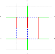
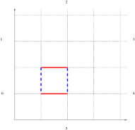
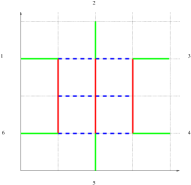
Figure 2: An example of an alternating path. Suppose we start with the FPL on the left and consider the alternating path of the figure on the right, we end up, after the operation of Lemma 4.1, with the FPL on the right.

We now make the conjecture made at the beginning of this section more precise.

Conjecture 4.2.

Given an FPL $f$ of size $n$ and an integer $i$ between $1$ and $2n$ there is a canonical algorithm to find an alternating path $L$, which leads to another FPL $g$ in which the paths from $i$ and $i+1$ are connected. This algorithm also leads to an integer $j$ which will be needed to find the inverse of this map.

5 Experiments

We have performed computer experiments using Maple to find the supposed bijection Conjecture 4.2 and present a set of programs in two packages titled RS and FPL. These packages are available from the homepages of the authors and the arXiv.

The simplest test of the above conjecture is to simply count the number of times each FPL is the output of the alternating path procedure. If each FPL occurs exactly $2n$ times, this is a hint that the algorithm is correct. Most of the algorithms work for $n=2$ and $n=3$. The first nontrivial test occurs for $n=4$ where there are 42 FPLs. This case is also original in the sense that there occurs an FPL with a loop inside. This forces the algorithm to be nontrivial.

The first comment is that the obvious algorithms for the conjectured alternating paths do not work. Neither choosing the first available alternating path (starting from the path beginning at $i$) nor choosing the smallest alternating path which connects $i$ to $i+1$ are well-defined operations. There do arise examples when $n\geq 5$ in which there are several paths beginning at the first edge, two of which have the same length. Similarly there are examples where there are multiple shortest alternating paths which lead to different final FPLs. This problem of choice in proving the Razumov-Stroganov conjecture has been noticed before [10].

The second comment is that one can use the dihedral symmetry inherent in the FPL picture proved in [11]. If one has a prescribed alternating path algorithm for a certain FPL $f$ and an integer $i$ $(f,i)\to(g,j)$, then one can use the rotation defined in [11] to define the algorithm for $(f^{\prime},i+1)$ as $(g^{\prime},j+1)$. And similarly for the reflected case.

Another possible way out is to introduce “catalytic” sets. It is very possible that two sets ${\mathcal{A}}$ and ${\mathcal{B}}$ have the same cardinality without being in “natural bijection”, but there exist other sets ${\mathcal{C}}$ and ${\mathcal{D}}$, such that it is known that $|{\mathcal{C}}|=|{\mathcal{D}}|$ and there is a natural bijection between the Cartesian products ${\mathcal{A}}\times{\mathcal{C}}$ and ${\mathcal{B}}\times{\mathcal{D}}$. Similarly, if ${\mathcal{A}}\cup{\mathcal{C}}$ has a natural bijection with ${\mathcal{B}}\cup{\mathcal{D}}$. In other words, one has not to be a fanatic about “pure bijective proofs”, but view them merely as yet another tool that may be combined with other tools of the trade.

References

- [1] W.H. Mills, D.P. Robbins and H. Rumsey Jr., Alternating Sign Matrices and Descending Plane Partitions, J. Combin. Th. Ser. A 34 (1983), 340–359.
- [2] D. Zeilberger, Proof of the Alternating Sign Matrix Conjecture, Electronic J. Combin 3 no. 2 (1996), R13, 84pp.
- [3] G. Kuperberg, Another Proof of the Alternating-Sign Matrix Conjecture”, Internat. Math. Res. Notes No. 3 (1996), 139–150.
- [4] J. Propp, The many faces of alternating-sign matrices, preprint, arXiv:math/0208125.
- [5] B. Nienhuis, J. de Gier and M.T. Batchelor, The quantum symmetric XXZ chain at Delta=-1/2, alternating sign matrices and plane partitions, J. Phys. A 34 (2001), L265–L270.
-
[6]
A.V. Razumov and Yu.G. Stroganov, Spin chains and
combinatorics, J. Phys. A 34 (2001), 3185–3190.
A.V. Razumov and Yu.G. Stroganov, Combinatorial nature of ground state vector of O(1) loop model, Theor. Math. Phys. 138 (2004), 333–337,
A.V. Razumov and Yu.G. Stroganov, O(1) loop model with different boundary conditions and symmetry classes of alternating-sign matrices, Theor. Math. Phys. 142 (2005), 237–243. - [7] J. de Gier, Loops, matchings and alternating-sign matrices, Discr. Math. 298 (2005), 365–388.
-
[8]
P. Di Francesco, A refined Razumov-Stroganov conjecture,
J. Stat. Mech., P08009 (2004),
P. Di Francesco, A refined Razumov-Stroganov conjecture II, J. Stat. Mech., P11004 (2004), - [9] P. Zinn-Justin, Proof of Razumov-Stroganov conjecture for some infinite families of link patterns, preprint, arXiv:math/0607183
- [10] P. Di Francesco, Totally Symmetric Self-Complementary Plane Partitions and Quantum Knizhnik-Zamolodchikov equation: a conjecture, J. Stat. Mech., P09008 (2006).
- [11] B. Wieland, Large Dihedral Symmetry of the Set of Alternating Sign Matrices, Electronic J. Combin. 7 (2000), R37, 13 pp.