Bipartite states of low rank are
almost surely entangled

Abstract

We show that a bipartite state on a tensor product of two matrix algebras is almost surely entangled if its rank is not greater than that of one of its reduced density matrices.

1 Introduction

1.1 Background

Recently, Arveson [2] considered the question of when a bipartite mixed state of rank $r$ is almost surely entangled, and showed that this holds when $r\leq d/2$ where $d$ is the dimension of the smaller space. In this note we show that this result holds if $r\leq d$, with $d$ now the dimension of the larger space.

We will use results from [11] on entanglement breaking channels and exploit the well-known isomorphism between bipartite states and completely positive (CP) maps.. We will first consider states associated with completely positive trace-preserving (CPT maps) and then find that extension to arbitrary bipartite states is quite straightforward.

If the rank of a bipartite state $\gamma_{AB}$ is strictly smaller than that of either of its reduced density matrices, then the state must be entangled. This is an immediate consequence of well-known results on entanglement, and seems to have first appeared explicitly in [12]. We include a proof in Appendix A for completeness. This allows us to restrict attention to the case in which the ranks of the reduced density matrices are equal, with one of full rank.

Although it seems natural to expect that this result is optimal, recent results of Walgate and Scott [19] suggest otherwise. Let the Hilbert spaces ${\cal H}_{A}$ and ${\cal H}_{B}$ have dimensions $d_{A}$ and $d_{B}$ respectively. It follows from a result proved independently by Wallach [20] and by Parthasarathy [15] for multi-partite entanglement that when $s>(d_{A}-1)(d_{B}-1)$ any subspace of ${\cal H}_{AB}={\cal H}_{A}\otimes{\cal H}_{B}$ with dimension $s$ contains some product states, and that this bound is best possible, i.e., if $s\leq(d_{A}-1)(d_{B}-1)$ then there is some subspace of dimension $s$ with no product states.

Walgate and Scott extended this by proving [19, Corollary 3.5] that if a subspace of ${\cal H}_{A}\otimes{\cal H}_{B}$ has dimension $s\leq(d_{A}-1)(d_{B}-1)$ then, almost surely, it contains no product states. For a bipartite state $\gamma_{AB}$ with rank $r\leq(d_{A}-1)(d_{B}-1)$, it follows that range of $\gamma_{AB}$ almost surely contains no product states, which implies that a bipartite state $\gamma_{AB}$ with rank $r\leq(d_{A}-1)(d_{B}-1)$ is almost surely entangled. Alternatively, one could apply [19, Theorem 3.4] directly to $\ker(\gamma_{AB})$ to reach the same conclusion.

When $d_{A}>d_{B}\geq 2$, this result is stronger than ours, but for a pair of qubits, $d_{A}=d_{B}=2$ our result is stronger. Moreover, it is easy to extend our qubit results to the general case of bipartite states with rank $r=d_{A}\geq d_{B}\geq 2$, providing a proof quite different from that in [19]. Although our measure is constructed differently from that used in [2], our approach is similar in the sense that we show that in a natural parameterization of the set of density matrices, the separable ones lie in a space of smaller dimension.

In the next half of this section, we review relevant terminology, and describe the notation and conventions we will use. Qubit channels and states are considered in Section 2, and the general case in Section 3. We conclude with some remarks about other approaches, and the question of the largest rank for which the separable states have measure zero.

1.2 Basics and notation

In this paper, we consider maps $\Phi:{\cal B}({\cal H}_{A})\mapsto{\cal B}({\cal H}_{B})$ and identify them with bipartite states or, equivalently, density matrices in ${\cal B}({\cal H}_{A})\otimes{\cal B}({\cal H}_{B})$ via the Choi-Jamiolkowski isomorphism as described below. Our primary interest is the situation in which ${\cal H}_{A}={\bf C}_{d_{A}}$, in which case we can identify ${\cal B}({\bf C}_{d})$ with $M_{d}$, the space of $d\times d$ matrices. However, we will also have occasion to consider either Hilbert space ${\cal H}$ as a proper subspace of ${\bf C}_{d}$ for some $d$.

We will identify a state with a density matrix, i.e., a positive semi-definite operator $\rho$ with $\hbox{Tr}\,\rho=1$, in ${\cal B}({\cal H})$. To an operator algebraist this corresponds to the positive linear functional on the algebra ${\cal B}({\cal H})$ which takes $A\mapsto\hbox{Tr}\,\rho\,A$. In the physics and quantum information literature, a density matrix (or, more properly, a density operator) is often referred to as a (mixed) state on ${\cal H}$ (because the density operator acts on ${\cal H}$. )

When ${\cal H}_{A}={\bf C}_{d_{A}}$ and ${\cal H}_{B}={\bf C}_{d_{B}}$, we write $\Phi:M_{d_{A}}\mapsto M_{d_{B}}$. In this case, let $\{e_{j}\}$ and $\{f_{m}\}$ denote orthonormal bases for ${\bf C}_{d_{A}}$ and ${\bf C}_{d_{B}}$ respectively. The isomorphism between states and matrices arises from the fact that

$$\hbox{Tr}\,|f_{m}\rangle\langle f_{n}|\,\Phi(|e_{j}\rangle\langle e_{k}|)$$ (1)

can be interpreted as either

(i) the matrix representative of the linear map $\Phi:M_{d_{A}}\mapsto M_{d_{B}}$ in the bases $|f_{m}\rangle\langle f_{n}|$ and $|e_{j}\rangle\langle e_{k}|$ for $M_{d_{B}}$ and $M_{d_{A}}$ respectively, or,

(ii) the density matrix $\gamma_{AB}$ of a state on ${\bf C}_{d_{A}}\otimes{\bf C}_{d_{B}}$ with elements $[\gamma_{AB}]_{jm,kn}$ in the product basis $|e_{j}\otimes f_{m}\rangle$.

Conversely, any state on ${\bf C}_{d_{A}}\otimes{\bf C}_{d_{B}}$ defines a CP map. We describe this well-known fact in detail in order to establish some conventions for interpretations of $\gamma_{A}$ and $\gamma_{B}$. Observe that (ii) is equivalent to writing $\gamma_{AB}$ as a block matrix of the form

$$\gamma_{AB}=\tfrac{1}{d_{A}}\sum_{jk}{|e_{j}\rangle\langle e_{k}|}\otimes P_{jk}=\tfrac{1}{d_{A}}\sum_{jk}{|e_{j}\rangle\langle e_{k}|}\otimes\Phi(|e_{j}\rangle\langle e_{k}|)$$ (2)

with the block $P_{jk}=\Phi(|e_{j}\rangle\langle e_{k}|)$ the matrix in $M_{d_{B}}$ given by the image $\Phi(|e_{j}\rangle\langle e_{k}|)$. One can write an arbitrary matrix in $M_{d_{A}}\otimes M_{d_{B}}$ in the block form $\sum_{jk}|e_{j}\rangle\langle e_{k}|\,P_{jk}$ and then define $\Phi(|e_{j}\rangle\langle e_{k}|)=P_{jk}$ and extend by linearity or, equivalently,

$$\Phi(A)=\sum_{jk}a_{jk}P_{jk}$$ (3)

when $A=\sum_{jk}a_{jk}|e_{j}\rangle\langle e_{k}|$.

Observe that

$$\gamma_{B} = \tfrac{1}{d_{A}}\hbox{Tr}_{A}\gamma_{AB}=\tfrac{1}{d_{A}}\sum_{k}\Phi(|e_{k}\rangle\langle e_{k}|)=\tfrac{1}{d_{A}}\Phi(I_{A})$$ (4a)

$$\gamma_{A} = \tfrac{1}{d_{A}}\hbox{Tr}_{B}\gamma_{AB}=\tfrac{1}{d_{A}}\sum_{jk}|e_{j}\rangle\langle e_{k}|\,\hbox{Tr}\,\Phi(|e_{j}\rangle\langle e_{k}|)$$ (4b)

and that this implies the following:

a) $\Phi$ is unital, i.e., $\Phi(I_{A})=I_{B}$, if and only if $\gamma_{B}=\tfrac{1}{d_{A}}I_{B}$, and

b) $\Phi$ is trace-preserving (TP), i.e., $\hbox{Tr}_{B}\,\Phi(X)=\hbox{Tr}_{A}\,X~{}~{}\forall~{}X\in{\cal B}({\cal H}_{A})$, if and only if $\gamma_{A}=\tfrac{1}{d_{A}}I_{A}$.

When $M_{d}$ or ${\cal B}({\cal H})$ is equipped with the Hilbert-Schmidt inner product, one can define the adjoint, or dual, of a map $\Phi$. We denote this by $\widehat{\Phi}$ and observe that this is equivalent to

$$\hbox{Tr}\,B^{\dagger}\Phi(A)=\hbox{Tr}\,[\widehat{\Phi}(B)]^{\dagger}A.$$ (5)

A matrix $\Phi$ is TP if and only if its adjoint $\widehat{\Phi}$ is unital.

It is a consequence of Theorem 5 in [7] that the extreme points of the convex set of CP maps for which $\gamma_{A}=\widehat{\Phi}(I_{B})=\rho$ have a state representative (often called the Choi matrix) with rank $\leq$ rank $\rho$. We prefer to consider CPT maps and regard the density matrices with rank $\leq d_{A}$ as an extension of the set of extreme points. As shown in Appendix B, this corresponds to the closure of the set of of extreme points. We let ${\cal D}_{C}$ denote the set of density matrices in ${\cal B}({\cal H}_{C})$ or $M_{d_{C}}$ and ${\cal D}_{C}(r)$ to denote the subset of rank $r$. We also define the following subsets of ${\cal D}_{AB}(r)$.

$${\cal P}_{A}(\rho;r,s) \equiv \{\gamma_{AB}\in{\cal D}_{AB}:{\rm rank}\,\gamma_{AB}=r,~{}{\rm rank}\,\gamma_{A}=s~{}\hbox{and}~{}\gamma_{A}=\rho\}$$ (6a)

$${\cal P}_{A}(r,s) \equiv \{\gamma_{AB}\in{\cal D}_{AB}:{\rm rank}\,\gamma_{AB}=r~{}\hbox{and}~{}{\rm rank}\,\gamma_{A}=s\}$$ (6b)

Although the sets in (6) above are subsets of ${\cal D}_{AB}\subset{\cal B}({\cal H}_{A})\otimes{\cal B}({\cal H}_{B})\simeq M_{d_{A}}\otimes M_{d_{B}}$ we use the subscript $A$ to emphasize that we impose conditions only on the marginal $\gamma_{A}$. When rank $\rho_{1}=$ rank $\rho_{2}=d_{A}$, the map

$$\gamma_{AB}\mapsto(\rho_{2}^{1/2}\rho_{1}^{-1/2}\otimes I_{B})\gamma_{AB}\,(\rho_{1}^{-1/2}\rho_{2}^{1/2}\otimes I_{B})$$ (7)

gives an isomorphism from ${\cal P}_{A}(\rho_{1};r,d_{A})$ to ${\cal P}_{A}(\rho_{2};r,d_{A})$ and each of these is isomorphic to ${\cal P}_{A}(\tfrac{1}{d_{A}}I_{A};d_{A},d_{A})$ which is isomorphic to the set of CPT maps $\Phi$ whose Choi matrix has rank $d_{A}$. We will let ${\cal S}_{A}(\rho;r,s)$, etc. denote the corresponding subsets of separable state in (6).

It will be useful to introduce the notation $\Upsilon_{T}$ for the map that takes a density matrix $\rho\mapsto T^{\dagger}\rho T$.

2 Maps with qubit inputs

2.1 Canonical form and parameterization

Now consider the case of CPT maps on qubits for which ${\cal H}_{A}={\cal H}_{B}={\bf C}_{2}$. As observed in [14], these maps can be written using the Bloch sphere representation in the form

$$\Phi\big{(}w_{0}I+\sum_{k}w_{k}\sigma_{k}\big{)}=w_{0}I+\sum_{k}(t_{k}w_{0}+\lambda_{k}w_{k})\sigma_{k}$$ (8)

where $\sigma_{k}$ denote the three Pauli matrices. Necessary and sufficient conditions on $t_{k},\lambda_{k}$ which ensure that $\Phi$ is CP are given in [18]. The form (8) is equivalent to representing $\Phi$ by a matrix $T$ with elements $t_{jk}={\textstyle\frac{1}{2}}\hbox{Tr}\,\sigma_{j}\Phi(\sigma_{k})$ so that, with subscripts $j,k=0,1,2,3$ and the convention $I_{2}=\sigma_{0}$

$$T=\begin{pmatrix}1&0&0&0\\ t_{1}&\lambda_{1}&0&0\\ t_{2}&0&\lambda_{2}&0\\ t_{2}&0&0&\lambda_{3}\end{pmatrix}.$$ (9)

As shown in [14, Appendix B] an arbitrary unital map on qubits can be reduced to this form by applying a variant of the singular value decomposition to the $3\times 3$ submatrix with $j,k\in\{1,2,3\}$ using only real orthogonal rotations. Given the isomorphism between rotations and $2\times 2$ unitary matrices, this corresponds to making a change of basis on the input and output spaces ${\cal H}_{A}={\bf C}_{d_{A}}={\bf C}_{2}$ and ${\cal H}_{B}={\bf C}_{d_{B}}={\bf C}_{2}$ respectively. Thus, for an arbitrary unital CP map $\Phi$ one can find unitary $U,V$ such that $\Upsilon_{V^{\dagger}}\circ\Phi\circ\Upsilon_{U}$ has the form (8) or, equivalently, a matrix representative of the form (9).

It was shown in [18] that the maps with Choi rank $\leq 2$ are precisely those for which the form (9) becomes

$$T_{u,v}=\begin{pmatrix}1&0&0&0\\ 0&\cos u&0&0\\ 0&0&\cos v&0\\ \sin u\sin v&0&0&\cos u\cos v\end{pmatrix}$$ (10)

with $u,v$ in $(-\pi,\pi]\times[0,\pi]$. Moreover, as shown in [16], the entanglement breaking (EB) maps are precisely the channels which have either $\cos u=0$ or $\cos v=0$.

It follows from (10) that every element of ${\cal P}_{A}({\textstyle\frac{1}{2}}I;2,2)$ can be represented by a triple $\big{(}(u,v),U,V\big{)}$ consisting of a point in ${\bf R}_{2}$, and two unitary matrices $U,V$. However, some care must be taken so that each element of ${\cal P}_{A}({\textstyle\frac{1}{2}}I;2,2)$ is counted exactly once. It suffices to restrict $(u,v)$ to the rectangle

$$\overline{\Delta}=\big{[}0,\frac{\pi}{2}\big{]}\times\big{[}0,\frac{\pi}{2}\big{]}$$ (11)

Suitable rotations will give all allowed negative values of the non-zero elements in (10), as well as even permutations of $t_{k}$ and $\lambda_{k}$. Problems with overcounting occur only on the lines $u=0,v=0,u=v$. To deal with this we define

$$\Delta=\{(u,v):0<u\leq\frac{\pi}{2},0<v\leq\frac{\pi}{2},u\neq v\}.$$ (12)

(The line segments on the boundary with $u=\frac{\pi}{2}$ and $v=\frac{\pi}{2}$ are included in $\Delta$ as shown in Figure 1.)

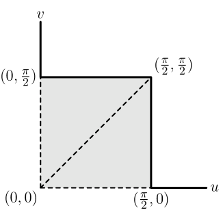
Figure 1: The rectangle $\overline{\Delta}$ corresponds to the shaded region. The dashed lines are not in $\Delta$. The lines $u=\frac{\pi}{2}$ and $v=\frac{\pi}{2}$ correspond to the EB channels.

Because different pairs of matrices $U,V$ may give the same channel on the lines not included in (12), we define equivalence classes as follows. Let ${\cal R}_{t}$ (with $t=x,y,z$) denote the subset of $SU(2)$ corresponding to the rotations around the indicated axis. We write $(U,V)\simeq(U^{\prime},V^{\prime})$ if there is an $R_{t}\in{\cal R}_{t}$ such that $U^{\prime}=R_{t}U$ and $V^{\prime}=R_{t}V$ or, equivalently $U^{\prime}U^{\dagger}=V^{\prime}V^{\dagger}\in{\cal R}_{t}$, and denote the quotient space $(SU(2)\times SU(2))/{\cal R}_{t}$. With this notation, we now make some observations

• The subset of EB channels consist of those channels for which either $u=\frac{\pi}{2}$ or $v=\frac{\pi}{2}$;

• The line $u=v$ corresponds to the amplitude damping channels (It is well-known that only the case $u=v=\frac{\pi}{2}$ is EB; this is a completely noisy channel mapping to a fixed pure state.) From (10) one sees that these channels are invariant under rotations about the $z$-axis, and the set of amplitude damping channels in ${\cal P}_{A}({\textstyle\frac{1}{2}}I;2,2)$ is isomorphic to $(u,u)\times(SU(2)\times SU(2))/{\cal R}_{z}$.

• The line segments with $u=0$ and $v=0$ correspond to phase-damping channels. From (10) one sees that these channels are invariant under rotations about the $x$ and $y$-axes respectively. Thus, the set of phase damping channels in ${\cal P}_{A}({\textstyle\frac{1}{2}}I;2,2)$ is isomorphic to

  $$\{(0,v):v\in(0,\tfrac{\pi}{2},]\}\times(SU(2)\times SU(2))/{\cal R}_{x}$$

  $$\bigcup \{(u,0):u\in(0,\tfrac{\pi}{2}]\}\times(SU(2)\times SU(2))/{\cal R}_{y}.$$

• The point $u=v=0$ gives the identity channel, for which rank $\gamma_{AB}=1$.

Thus ${\cal P}_{A}({\textstyle\frac{1}{2}}I;2,2)$ is isomorphic to

$$\Delta\times SU(2)\times SU(2)\,\bigcup\,\{(u,u)\}_{u\in(0,\frac{\pi}{2}]}\times(SU(2)\times SU(2))/{\cal R}_{z}\quad$$

$$\bigcup\,\{(u,0)\}_{u\in(0,\frac{\pi}{2}]}\times(SU(2)\times SU(2))/{\cal R}_{y}$$ (13)

$$\bigcup\,\{(0,v)\}_{v\in(0,\frac{\pi}{2}]}\times(SU(2)\times SU(2))/{\cal R}_{x}$$

and, ${\cal S}_{A}({\textstyle\frac{1}{2}}I;2,2)$, the subset of EB channels in ${\cal P}_{A}({\textstyle\frac{1}{2}}I;2,2)$, is isomorphic to

$$\{(u,\tfrac{\pi}{2}):u\in(0,\tfrac{\pi}{2})\}\times SU(2)\times SU(2)$$ (14)

$$\,\bigcup\,\{(\tfrac{\pi}{2},v):v\in(0,\tfrac{\pi}{2})\}\times SU(2)\times SU(2)\bigcup\,(0,\frac{\pi}{2})\times(SU(2)\times SU(2))/{\cal R}_{x}\quad$$

$$\,\bigcup\,(\frac{\pi}{2},0)\times(SU(2)\times SU(2))/{\cal R}_{y}\,\bigcup\,(\frac{\pi}{2},\frac{\pi}{2})\times(SU(2)\times SU(2))/{\cal R}_{z}.$$

2.2 Construction of a measure

Let $m_{2}$ be the normalized Lebegue measure on $\overline{\Delta}$ and $\nu_{2}$ the normalized Haar measure on $SU(2)$. Then the product measure $\widetilde{\mu}\equiv m_{2}\times\nu_{2}\times\nu_{2}$ defines a probability measure on $\Omega_{2}=\overline{\Delta}\times SU(2)\times SU(2)$. Although every point in $\Omega_{2}$ corresponds to an element in ${\cal P}_{A}({\textstyle\frac{1}{2}}I;2,2)$, it can happen, as described above, that more than one point corresponds to the same CPT map $\Phi$. Therefore, to define a measure on ${\cal P}_{A}({\textstyle\frac{1}{2}}I;2,2)$ we use the map $g:\Omega_{2}\rightarrow{\cal P}_{A}({\textstyle\frac{1}{2}}I;2,2)$ which takes

$$\big{(}(u,v),U,V\Big{)}\mapsto\Upsilon_{V}\circ\Phi_{u,v}\circ\Upsilon_{U^{\dagger}}$$ (15)

where $\Phi_{u,v}$ denotes the CPT map whose Choi matrix is given by (10). The map $g$ is surjective which allows us to define a measure $\mu$ on all sets $X\subset{\cal P}_{A}({\textstyle\frac{1}{2}}I;2,2)$ for which $g^{-1}(X)$ is measurable by

$$\mu(X)=\widetilde{\mu}\left(g^{-1}(X)\right).$$ (16)

Since $g$ is surjective, $g^{-1}({\cal P}_{A}({\textstyle\frac{1}{2}}I;2,2))=\Omega_{2}$ which implies that ${\cal P}_{A}({\textstyle\frac{1}{2}}I;2,2)$ is measurable and $\mu({\cal P}_{A}({\textstyle\frac{1}{2}}I;2,2)=1$. Thus, $\mu$ is a probability measure on ${\cal P}_{A}({\textstyle\frac{1}{2}}I;2,2)$

Moreover, the entanglement breaking channels satisfy

$$\mu({\cal S}_{A}({\textstyle\frac{1}{2}}I;2,2))$$ (17)

$$= \widetilde{\mu}\big{(}\{(u,\tfrac{\pi}{2}):u\in[0,\tfrac{\pi}{2}]\}\times SU(2)\times SU(2)\cup\{(\tfrac{\pi}{2},v):v\in[0,\tfrac{\pi}{2}\}\times SU(2)\times SU(2)\big{)}$$

$$= 0\cdot 1\cdot 1+0\cdot 1\cdot 1=0$$

Thus, we have proved the following

Theorem 1

A CPT map $\Phi:M_{2}\mapsto M_{2}$ of Choi-rank 2 is almost surely not EB, or, equivalently, a state $\gamma_{AB}$ on ${\bf C}_{2}\otimes{\bf C}_{2}$ which has rank 2 and $\gamma_{A}={\textstyle\frac{1}{2}}I$ is almost surely entangled.

Since, the unitary conjugations have Choi matrices of rank 1, and correspond to the set $(0,0)\times SU(2)$ which has measure zero, we have also proved the following result, which we state for completeness.

Theorem 2

A CPT map $\Phi:M_{2}\mapsto M_{2}$ of Choi-rank $\leq 2$ is almost surely not EB, or, equivalently, a state $\gamma_{AB}$ on ${\bf C}_{2}\otimes{\bf C}_{2}$ which has rank $\leq 2$ and $\gamma_{A}={\textstyle\frac{1}{2}}I$ is almost surely entangled.

2.3 Removing the TP restriction

We would like to extend the results of the previous section to

Theorem 3

If a state $\gamma_{AB}$ on ${\bf C}_{2}\otimes{\bf C}_{2}$ has rank 2 and $\gamma_{A}$ also has rank 2, then $\gamma_{AB}$ is almost surely entangled.

Proof: As observed after (7), ${\cal P}_{A}(\rho_{1};r,d_{A})\simeq{\cal P}_{A}(\rho_{2};r,d_{A})$; Indeed, the CP maps corresponding to states in ${\cal D}_{A}(\rho;2,2)$ have the form $\Phi\circ\Upsilon_{\sqrt{2\rho}}$ with $\Phi$ CPT, although it might seem more natural to consider the dual $\Upsilon_{\sqrt{2\rho}}\circ\widehat{\Phi}$ which takes $I\mapsto d_{A}\,\rho$. Next, observe that any density matrix $\rho\in M_{d_{A}}$ of rank 2, can be written as $U\left(\begin{smallmatrix}x&0\\ 0&1-x\end{smallmatrix}\right)U^{\dagger}$ with $x\in(0,{\textstyle\frac{1}{2}})$ and $U\in SU(2)$; the case $x={\textstyle\frac{1}{2}}$ gives ${\textstyle\frac{1}{2}}I$ independent of $U$. Thus the set of density matrices $\rho\in M_{d_{A}}$ of rank 2 is isomorphic to

$${\textstyle\frac{1}{2}}I~{}\cup~{}(0,{\textstyle\frac{1}{2}})\times SU(2)$$ (18)

and the set of bipartite density matrices ${\cal P}_{A}(2,2)$ (for which rank $\gamma_{AB}=$ rank $\gamma_{A}=2$) is isomorphic to

$${\cal P}_{A}({\textstyle\frac{1}{2}}I;2,2)\bigcup{\cal P}_{A}({\textstyle\frac{1}{2}}I;2,2)\times(0,{\textstyle\frac{1}{2}})\times SU(2).$$ (19)

To define a measure on this set, let $m_{1}$ denote normalized Lebesque measure on $(0,{\textstyle\frac{1}{2}})$ and let $\lambda_{2,t}$ be defined using product measure so that

$$\lambda_{2,t}(X)=\begin{cases}t\,(\mu\times m_{1}\times\nu_{2})(X)&~{}~{}X\in{\cal P}_{A}({\textstyle\frac{1}{2}}I;2,2)\times(0,{\textstyle\frac{1}{2}})\times SU(2)\\ (1\!-\!t)\,\mu(X)&~{}~{}X\in{\cal P}_{A}({\textstyle\frac{1}{2}}I;2,2)\end{cases}$$ (20)

where we can pick any $t\in(0,1]$ and $\mu$ is the measure defined in Section 2.2. Then the subset of EB channels ${\cal S}_{A}(2,2)$ has measure

$$\lambda_{2,t}\big{(}{\cal S}_{A}(2,2)\big{)} = \mu\big{(}{\cal S}_{A}({\textstyle\frac{1}{2}}I;2,2)\big{)}+\mu\big{(}{\cal S}_{A}({\textstyle\frac{1}{2}}I;2,2)\big{)}\,m_{1}(0,{\textstyle\frac{1}{2}})\,\nu_{2}\big{(}SU(2)\big{)}$$ (21)

$$= t\cdot 0+(1\!-\!t)\cdot 0\cdot 1\cdot 1=0\qquad\qquad{\bf QED}$$

independent of $t\in(0,1])$. We can drop the requirement that $\gamma_{A}$ has rank 2 by observing that extension to all $\gamma_{AB}$ of rank 2 requires only that one replaces $(0,{\textstyle\frac{1}{2}})$ on the right side of (19) by $[0,{\textstyle\frac{1}{2}})$. Thus, we can conclude that

Corollary 4

If a state $\gamma_{AB}$ on ${\bf C}_{2}\otimes{\bf C}_{2}$ has rank 2, then $\gamma_{AB}$ is almost surely entangled.

2.4 Two-dimensional subspaces of ${\bf C}_{d}$.

We can use the isomorphism between ${\bf C}_{2}$ and any Hilbert space of dimension 2 to replace either ${\cal H}_{A}$ or ${\cal H}_{B}$ by a two dimensional subspace of ${\bf C}_{d}$. However, for later use, we now want to extend our qubit results to the somewhat more general situation of the set of all CPT maps $\Phi:{\bf C}_{2}\mapsto{\bf C}_{d_{B}}$ whose range has the form ${\cal B}\big{(}\hbox{span}\,\{|v_{1}\rangle,|v_{2}\rangle\}\big{)}$ with $|v_{1}\rangle,|v_{2}\rangle\in{\bf C}_{d_{B}}$. Here, we do not fix the range, but consider all CPT maps whose range corresponds to some two-dimensional subspace of ${\bf C}_{d_{B}}$.

Observe that in the polar decomposition $\Upsilon_{V^{\dagger}}\circ\Phi\circ\Upsilon_{U}$ leading to the canonical form (8) we need only replace $V$ by an isometry $V:{\bf C}_{2}\mapsto{\cal H}_{B}$. Then in (2.1) and (14), the first use of $SU(2)$ in each subset must be replaced by ${\cal V}_{d}$ which is defined as the subset of $d\times 2$ matrices satisfying $V^{\dagger}V=I_{2}$. By Theorem A.2 of [2], ${\cal V}_{d}$ can be given the structure of a real analytic manifold with a probaility measure $v_{d}$ (which is unique if it is required to be left-invariant under $SU(d)$). Although ${\cal V}$ is not a group, we can define equivalence classes as before with$(V,U)\simeq(V^{\prime},U^{\prime})$ if there is a $R_{t}\in{\cal R}_{t}$ such that $V^{\prime}=VR_{t}$ and $U^{\prime}=UR_{t}$. Then the previous arguments go through with $SU(2)\times SU(2)$ replaced by ${\cal V}_{d}\times SU(2)$ in Section 2.1 and the corresponding use of $\nu_{2}$ in Section 2.2 by $v_{d}$.

3 General maps

3.1 CPT maps with $d_{A}>2$.

We now assume $d_{A}\geq d_{B}\geq 2$ and extend these results to bipartite states on ${\bf C}_{d_{A}}\otimes{\bf C}_{d_{B}}$ with $\gamma_{A}=\tfrac{1}{d_{A}}I_{A}$. We begin by considering a CPT map $\Phi:M_{d_{A}}\mapsto M_{d_{B}}$ with Choi-rank $d_{A}$. By Theorem 5C of [11], which is equivalent to Corollary 14, $\Phi$ can always be written in the form

$$\Phi(\rho)=\sum_{k}|g_{k}\rangle\langle g_{k}|\langle\psi_{k},\rho\,\psi_{k}\rangle$$ (22)

where $\{g_{k}\}$ is an orthonormal basis for ${\bf C}_{d_{A}}$, but the states $\psi_{k}\in{\bf C}_{d_{B}}$ need not be orthogonal or even linearly independent. In the basis $g_{k}$, the Choi matrix for $\Phi$ has the form

$$\gamma_{AB}=\tfrac{1}{d_{A}}\sum_{k}|g_{k}\rangle\langle g_{k}|\otimes|\psi_{k}\rangle\langle\psi_{k}|$$ (23)

which implies that $\gamma_{AB}$ is block diagonal with each block a $d_{B}\times d_{B}$ rank one projection. Let us first assume that $\psi_{1}$ and $\psi_{2}$ are linearly independent.

Now let $P_{k}\equiv|\psi_{k}\rangle\langle\psi_{k}|$ and write (23) explicitly in block form, as

$$\gamma_{AB}=\tfrac{1}{d_{A}}\begin{pmatrix}P_{1}&0&0&0&\ldots&0\\ 0&P_{2}&0&0&\ldots&0\\ 0&0&P_{3}&0&\ldots&0\\ \vdots&&&\ddots&&\vdots\\ 0&0&\ldots&0&\ldots&P_{d_{A}}\end{pmatrix}$$ (24)

and consider a density matrix of the form

$$\tfrac{1}{d_{A}}\begin{pmatrix}Q&0&0&\ldots&0\\ 0&P_{3}&0&\ldots&0\\ \vdots&&\ddots&&\vdots\\ 0&\ldots&0&\ldots&P_{d_{A}}\end{pmatrix}$$ (25)

where $Q\in M_{2}\otimes M_{d_{B}}$ is a positive semi-definite $2d_{B}\times 2d_{B}$ matrix of rank 2 satisfying $\hbox{Tr}_{B}\,Q=I_{2}$. Now a density matrix of the form (25) is separable if and only if ${\textstyle\frac{1}{2}}Q$ is separable. However, ${\textstyle\frac{1}{2}}Q$ is a density matrix of the form considered in Section 2.4.

Let ${\cal Y}_{d_{A}}(\{g_{k}\},\{\psi_{k}\})$ denote the subset of ${\cal P}_{A}(\tfrac{1}{d_{A}}I_{A};d_{A},d_{A},)$ consisting of density matrices of the form (25) or, equivalently,

$${\cal Y}_{d_{A}}(\{g_{k}\},\{\psi_{k}\})=\Big{\{}Q\oplus\sum_{k=3}^{d_{A}}|g_{k}\rangle\langle g_{k}|\otimes|\psi_{k}\rangle\langle\psi_{k}|:Q\in{\cal X}_{AB},\hbox{Tr}_{B}\,Q=I_{2}\big{\}}$$ (26)

where $\oplus$ denotes the direct sum and

$${\cal X}_{AB}={\cal B}\big{(}\hbox{span}\{|g_{1}\rangle,|g_{2}\rangle\}\otimes{\cal B}\big{(}\hbox{span}\{|\psi_{1}\rangle,|\psi_{2}\rangle\}\big{)}.$$ (27)

The set of projections $|\psi_{k}\rangle\langle\psi_{k}|\in M_{d_{B}}$ is isomorphic to $S_{2d_{B}-1}$, the $\ell_{2}$ unit sphere in ${\bf R}_{2d_{B}}$. For a given $|g_{1}\rangle,|g_{2}\rangle$, the set ${\cal X}_{AB}$ depends only on span $\{|\psi_{1}\rangle,|\psi_{2}\rangle\}$ and not the choice of individual vectors. Therefore, we can identify each point in

$$\Omega_{d_{A}} \equiv \overline{\Delta}_{2}\times{\cal V}_{d_{B}}\times SU(2)\times SU(d_{A})/SU(2)\times\underset{d_{A}-2}{\underbrace{S_{2d_{B}-1}\times\ldots\times S_{2d_{B}-1}}}$$ (28)

$$= \overline{\Delta}_{2}\times{\cal V}_{d_{B}}\times SU(d_{A})\times\underset{d_{A}-2}{\underbrace{S_{2d_{B}-1}\times\ldots\times S_{2d_{B}-1}}}$$

with a density matrix $\gamma_{AB}$ in ${\cal Y}_{d_{A}}\equiv\bigcup_{\{g_{k}\},\{\psi_{k}\}}{\cal Y}_{d_{A}}(\{g_{k}\},\{\psi_{k}\})$, the set of all density matrices of the form (25). (Note that $S_{2d_{B}-1}$ occurs $d_{A}-2$ times in (28) corresponding to the choices of $\psi_{k}$ for $k=3,4\ldots n$. The set ${\cal Y}_{d_{A}}(\{g_{k}\},\{\psi_{k}\})$ depends only on span $\{|\psi_{1}\rangle,|\psi_{2}\rangle\}=$ range $V$ with $V\in{\cal V}_{d_{B}}$, with non-orthogonal vectors $|\psi_{1}\rangle,|\psi_{2}\rangle$ associated with non-unital qubit channels via isomorphism.)

Let $m_{2}$ and $v_{d}$ be measures as in Sections 2.2 and 2.4, let $\nu_{d}$ be normalized Haar measure on $SU(d)$ and let $n_{2d_{B}-1}$ be a probability measure on $S_{2d_{B}-1}$. We define a normalized measure $\widetilde{\mu}$ on $\Omega_{d_{A}}$ by the product measure

$$\widetilde{\mu}=m_{2}\times v_{d_{B}}\times\nu_{2}\times\nu_{d_{A}/2}\times\underset{d_{A}-2}{\underbrace{n_{2d_{B}-1}\times\ldots\times n_{2d_{B}-1}}}$$ (29)

To obtain a measure on ${\cal Y}_{d_{A}}$ we proceed as in Section 2.2. Let $G:\Omega_{d_{A}}\mapsto{\cal Y}_{d_{A}}$ be the map that sends an element $\big{(}(u,v),V,U,|\psi_{3}\rangle,\dots,|\psi_{d_{A}}\rangle\big{)}$ to the corresponding density matrix in ${\cal Y}_{d_{A}}$ and define

$$\mu(X)=\widetilde{\mu}\big{(}G^{-1}(X)\big{)}$$ (30)

whenever $X\subset{\cal Y}_{d_{A}}$ for which $G^{-1}(X)$ is measurable.

As explained above, Corollary 14 implies that ${\cal S}_{A}(\tfrac{1}{d_{A}}I_{A};d_{A},d_{A})\subset{\cal Y}_{d_{A}}$. Then, proceeding as in (17), one finds

$$\mu\big{(}{\cal S}_{A}(\tfrac{1}{d_{A}}I_{A};d_{A},d_{A})\big{)}=0\cdot 1\cdot 1\cdot 1^{d_{A}-2}=0.$$ (31)

Moreover, for any reasonable extension of $\mu$ from ${\cal Y}_{d_{A}}$ to all of ${\cal P}_{A}(\tfrac{1}{d_{A}}I_{A},;d_{A},d_{A})$, the EB subset will still have measure zero. In particular, one could simply let

$$\omega(X)=\begin{cases}\mu(X)&\quad\hbox{if}\quad X\subset{\cal Y}_{d_{A}}\\ 0&\quad\hbox{if}\quad X\subset{\cal P}_{A}(\tfrac{1}{d_{A}}I_{d};d_{A},d_{A})\backslash{\cal Y}_{d_{A}}\end{cases}$$ (32)

and note that $\omega$ is absolutely continuous with respect to any other extension of $\mu$.

Thus, we have reduced the general case to that of $d_{A}=2$ and conclude that

Theorem 5

Let $\gamma_{AB}$ be a state on ${\bf C}_{d_{A}}\otimes{\bf C}_{d_{B}}$ which has rank $d_{A}\geq d_{B}\geq 2$ and for which $\gamma_{A}=\tfrac{1}{d_{A}}I_{A}$. Then $\gamma_{AB}$ is almost surely entangled.

Remark: The assumption that $\psi_{1}$ and $\psi_{2}$ are linearly independent can be dropped because that case corresponds to $u=v=\tfrac{\pi}{2}$ in (8) and is included implicitly in our analysis. The set of channels for which all $\psi_{j}$ are identical also has measure zero, except for the excluded situation $d_{B}=1$, for which all states are separable.

3.2 Reduction of the general case to CPT

As observed earlier, when rank $\rho=d_{A}$

$${\cal P}_{A}(\rho;d_{A},d_{A})=\big{\{}(\sqrt{d_{A}\,\rho}\otimes I_{B})\gamma_{AB}(\sqrt{d_{A}\,\rho}\otimes I_{B}):\gamma_{AB}\in{\cal P}_{A}(\tfrac{1}{d_{A}}I_{A};d_{A},d_{A})\}$$ (33)

is isomorphic to ${\cal P}_{A}(\tfrac{1}{d_{A}}I_{A};d_{A},d_{A})$. But parameterizing the set of density matrices of rank $d_{A}$ is a bit more subtle than for $d_{A}=2$ because of the need to consider degenerate eigenvalues, for situations beyond $\tfrac{1}{d_{A}}I$. However, this only affects a set of measure zero and can be dealt with as in the preceding sections. To describe the set of density matrix of rank $d_{A}$ consider the set of vectors

$$Z=\Big{\{}{\bf z}=(\zeta_{1},\zeta_{2},\ldots\zeta_{d_{A}}):0<\zeta_{1}\leq\zeta_{2}\leq\ldots\leq\zeta_{d_{A}},\sum_{k}\zeta_{k}=1\Big{\}}$$ (34)

in the positive facet of the $\ell_{1}$ unit ball of ${\bf R}_{d_{A}}$. We can associate each ${\bf z}\in Z$ with a diagonal matrix $\Lambda_{\bf z}$ so that that the map $h:({\bf z},U)\mapsto U\Lambda_{\bf z}U^{\dagger}$ takes $Z\times SU(d_{A})$ onto ${\cal D}_{A}(d_{A})$, the set of density matrices in $M_{d_{A}}$ with full rank $d_{A}$. Since we can identify $Z$ with a subset of ${\bf R}_{d_{A}-1}$, we put normalized Lebesque measure $m_{d_{A}-1}$ on $Z$, and let

$$\eta_{d_{A}}(X)=(m_{d_{A}-1}\times\nu_{d_{A}})(h^{-1}(X))$$ (35)

whenever $X\subset{\cal D}_{A}(d_{A})$ and $h^{-1}(X)$ is measurable. Then it follows from (31) that for any extension $\omega$ of $\mu$, the product measure $\omega\times\eta_{d_{A}}$ gives a measure on ${\cal P}_{A}(d_{A},d_{A})$ for which the separable states ${\cal S}_{A}(d_{A},d_{A})$ have measure $0\cdot 1=0$. Thus, we have proved

Theorem 6

If a state $\gamma_{AB}$ on ${\bf C}_{d_{A}}\otimes{\bf C}_{d_{B}}$ has rank $d_{A}\geq d_{B}\geq 2$ and rank$(\gamma_{A})=d_{A}$ then $\gamma_{AB}$ is almost surely entangled.

3.3 Further results

Theorem 11 states that if the rank of $\gamma_{A}$ is $d_{A}$ and the rank of $\gamma_{AB}$ is strictly smaller than $d_{A}$, then $\gamma_{AB}$ is entangled. Thus $r<d_{A}$ implies that ${\cal P}_{A}(\rho;r,d_{A})$ consists entirely of entangled states. If we combine this with our results for $r=s=d_{A}$ we obtain several additional theorems, which we state for completeness.

Theorem 7

Assume $d_{A}\geq d_{B}\geq 2$. If a state $\gamma_{AB}$ on $M_{d_{A}}\otimes M_{d_{B}}$ has rank $\gamma_{AB}\leq d_{A}=$ rank $\gamma_{A}$, then $\gamma_{AB}$ is almost surely entangled.

By using the isomorphism between ${\bf C_{d}}$ and any Hilbert space of dimension $d$ we can restate this by letting ${\cal H}_{A}=$ range $\gamma_{A}$ and ${\cal H}_{B}=$ range $\gamma_{B}$ and considering $\gamma_{AB}$ as a state on ${\cal B}({\cal H}_{A})\otimes{\cal B}({\cal H}_{A})$.

Theorem 8

If a state $\gamma_{AB}$ on $M_{d_{A}}\otimes M_{d_{B}}$ has rank $\gamma_{AB}\leq$ rank $\gamma_{A}$ and rank $\gamma_{A}\geq$ rank $\gamma_{B}\geq 2$, then $\gamma_{AB}$ is almost surely entangled.

We also find that we can eliminate the need to consider the rank of $\gamma_{A}$.

Theorem 9

Assume $d_{A}\geq d_{B}\geq 2$. If a state $\gamma_{AB}$ on $M_{d_{A}}\otimes M_{d_{B}}$ has rank $\gamma_{AB}\leq d_{A}$, then $\gamma_{AB}$ is almost surely entangled.

Proof: Let $\overline{Z}$ denote the closure of (34). Since this simply replaces the strict inequality $0<\zeta_{1}$ by $0\leq\zeta_{1}$, the set $\overline{Z}\times SU(d)$ includes all density matrices in $M_{d_{A}}$ so that

$$\overline{Z}\backslash Z\times SU(2)=h^{-1}\big{(}\{\rho\in{\cal P}_{A}:~{}\hbox{rank}~{}\rho<d_{A}\}\big{)}$$ (36)

Now extend the measure $\eta$ in (35) to all of ${\cal D}_{A}$. The set of all separable states $\gamma_{AB}$ with rank $\gamma_{AB}\leq d_{A}$ is ${\cal S}_{A}(d_{A})\equiv\bigcup_{s\leq d_{A}}{\cal S}_{d_{A}}(d_{A},s)$. The subset of separable states with rank $\gamma_{A}<d_{A}$ satisfies

$$\bigcup_{s<d_{A}}{\cal S}_{d_{A}}(d_{A},s)\subset\{\rho\in{\cal P}_{A}:~{}\hbox{rank}~{}\rho<d_{A}\}$$ (37)

But

$$\eta_{d_{A}}\big{(}\{\rho\in{\cal P}_{A}:~{}\hbox{rank}~{}\rho<d_{A}\}\big{)}=m_{d_{A}-1}(\overline{Z}\backslash Z)~{}\nu_{d_{A}}(SU(2))=0\cdot 1.$$ (38)

Thus

$$(\omega_{d_{A}}\times\eta_{d_{A}})\big{(}{\cal S}(d_{A})\big{)} = (\omega_{d_{A}}\times\eta_{d_{A}})\big{(}{\cal S}_{d_{A}}(d_{A},d_{A})\big{)}+(\omega_{d_{A}}\times\eta_{d_{A}})\Big{(}\bigcup_{s<d_{A}}{\cal S}_{d_{A}}(d_{A},s)\Big{)}$$ (39)

$$\leq 0\cdot 1+1\cdot 0=0\qquad\qquad{\bf QED}$$

4 Final comments

4.1 Remarks on measure

If we apply the argument used in to prove Theorem 9 to the subset of states with $\gamma_{A}=\tfrac{1}{d_{A}}I_{d_{A}}$ or equivalently, combine Theorems 5 and 11 we obtain the following result which we state in terms of channels.

Corollary 10

Assume $d_{A}\geq d_{B}\geq 2$. Then the set of CPT maps $\Phi:{\bf C}_{d_{A}}\mapsto{\bf C}_{d_{B}}$ whose Choi matrix has rank $r\leq d_{A}$ is almost surely entanglement breaking.

As shown in Appendix B, the closure of the set of extreme points of CPT maps $\Phi:{\bf C}_{d_{A}}\mapsto{\bf C}_{d_{B}}$ is precisely the set of channels whose Choi matrix has rank $\leq d_{A}$. Because the extreme points of a convex set lie on the boundary, their closure always has measure zero. Thus, Corollay 10 is a special case of a well known, more general fact from convex geometry. An alternative, and somewhat simpler, approach to proving Theorem 5, would be to use this fact together with Theorem 15. However, we feel that it is useful to see the specific paramaterizations which lead to our results. In our approach, one sees that everything really follows from the basic paramaterization of extreme points for qubit channels, and the fact that (up to sets of measure zero) the relevant sets of bipartite states can be parameterized as direct products on which we can put product measures.

One could extend Corollary 10 to the set of CP maps for which $\widehat{\Phi}(I_{B})=\rho$ with $\rho\in{\cal D}_{A}(r)$ fixed, again using the fact that the closure of the set of extreme points has measure zero. Then we can conclude that the subset of separable states $\cup_{s\leq r}{\cal S}(\rho;r,s)$ has measure zero with respect to a measure on $\cup_{s\leq r}{\cal P}(\rho;r,s)$. However, we can not go directly from this observation to Theorem 9 by taking the $\bigcup_{\rho\in{\cal D}_{A}}$ because the set ${\cal D}_{A}$ is uncountable. One would still need the argument in Section 3.2. What this observation about extreme points does tell us is that our results are not sensitive to the choice of measure. The fundamental issue is that the bipartite states can be parameterized as a smooth manifold on which the separable ones correspond to a space of smaller dimensions.

There is one unsatisfying aspect of using the the inverse image to define a measure, as in (16); namely, that it does not reflect the fact that different unitaries give the same map on some lines in $\overline{\Delta}$. An alternative would be to first define separate measures on the different regions in (2.1), e.g., on $\{(u,u)\}_{u\in(0,\tfrac{\pi}{2}]}\times(SU(2)\times SU(2))/{\cal R}_{z}$, use the product measure $m_{1}\times\widetilde{\nu}_{z}$ where $m_{1}$ is normalized Lebesque measure on $(0,\tfrac{\pi}{2)}$ and $\widetilde{\nu}_{z}$ is Haar measure on the group $(SU(2)\times SU(2))/{\cal R}_{z}$. One could then combine the measures on the four subsets in (2.1) as in (20) using, say, weights $1-t_{x}-t_{y}-t_{z},t_{z},t_{x},t_{y}$ with $t_{m}\geq 0$ and $\sum_{m=1}^{3}t_{m}\leq 1$. However, given that each of the line segments with $u=\tfrac{\pi}{2}$, $u=v$, and $v=\tfrac{\pi}{2}$ have measure zero in $\overline{\Delta}$, the most natural choice weight would be $t_{m}=0$, equivalent to simply omitting the corresponding channels (or states).

In fact, all regions which a quotient space is needed, as in Sections 2.2 and 3.2 have measure zero in our inverse image approach. Intuitively, one would like to simply observe that we can identify ${\cal D}_{A}({\textstyle\frac{1}{2}}I;2,2)$ with a subset of $[0,\tfrac{\pi}{2}]\times[0,\tfrac{\pi}{2}]$ that satisfies $\Delta\subset{\cal D}_{A}({\textstyle\frac{1}{2}}I;2,2)\subset\overline{\Delta}$ and then observe that since

$$\mu(\Delta)\leq\mu\big{(}{\cal D}_{A}({\textstyle\frac{1}{2}}I;2,2)\big{)}\leq\mu(\overline{\Delta}).$$ (40)

and $\mu(\Delta)=\mu(\overline{\Delta})=1$, one must have $\mu\big{(}{\cal D}_{A}({\textstyle\frac{1}{2}}I;2,2)=1$. But to use this approach, one must establish that ${\cal D}_{A}({\textstyle\frac{1}{2}}I;2,2)$ can be identified with a measurable subset of $\overline{\Delta}$.

4.2 Optimality

It is natural to ask if the results in Theorems 7 and 8 are optimal. For $d_{A}>2$, it is clear that the results which follow from those of Walgate and Scott [19] are better. Thus, the question becomes whether or not rank $\gamma_{AB}\leq(d_{A}-1)(d_{B}-1)$ is optimal. This does not follow from the subspace theorems in [19] because when rank $\gamma_{AB}=2>(d_{A}-1)(d_{B}-1)$ the product states can form a set of measure zero in a subspace of ${\cal H}_{A}\otimes{\cal H}_{B}$. However, we know that the separable ball in ${\cal B}({\cal H}_{A}\otimes{\cal H}_{B})$ has strictly positive measure [4, 5, 21] so that the optimal rank must be strictly smaller than $d_{A}d_{B}$.

In the case of qubits, we know that Theorem 3 is stronger than the results implied by Walgate and Scott [19], and that when rank $\gamma_{AB}=4$, the separable states have strictly positive measure. If we restrict attention to those states $\gamma_{AB}$ with rank 3 and $\gamma_{A}=\gamma_{B}={\textstyle\frac{1}{2}}I$ or, equivalently, the unital CPT maps with Choi-rank 3, we can use the familiar picture of a tetrahedron [8, 16, 18]. The rank 3 states correspond to the faces, and the subset of separable states on each face to the smaller triangle whose vertices are midpoints of the edges as shown in Figure 2. Thus, the unital CPT maps with Choi-rank 3 have measure $0.25$ with respect to all the unital CPT maps on qubits. However, it is open whether or not this holds when the restriction to unital maps is removed. Thus, the question of whether ${\cal P}_{A}({\textstyle\frac{1}{2}}I;3,2)$ has measure zero or positive measure seems to be open.

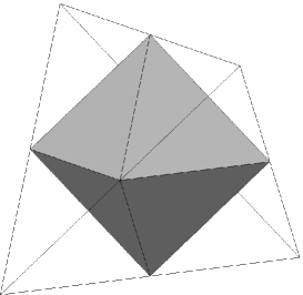
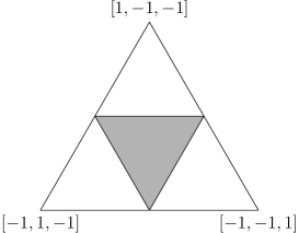
Figure 2: The left figure shows the tetrahedron of unital qubit channels with the octahedron the EB subset. The right figure shows one of the faces of the tetrahedron, corresponding to channels with Choi-rank 3, with the shaded region the subset of EB channels

Acknowledgment: It is a pleasure to thank Jonathon Walgate for bringing [19] to our attention, to Michael Wolf for providing reference [12] and to Michael Nathanson for assistance with figures.

Appendix A Some separability theorems

For completeness, we now state and sketch proofs of some results that are well known and/or proved in [11]. The first result appeared as [12, Theorem 1] in a slightly stronger form.

Theorem 11

If rank $\gamma_{AB}<d_{A}=~{}\hbox{rank}~{}\gamma_{A}$, then $\gamma_{AB}$ is not separable.

Proof: First observe that $\gamma_{AB}$ is separable if and only if

$$\widetilde{\gamma}_{AB}\equiv\tfrac{1}{d_{A}}(I_{A}\otimes\gamma_{A})^{-1/2}\gamma_{AB}(I_{A}\otimes\gamma_{A})^{-1/2}$$ (41)

is separable. But $\widetilde{\gamma}_{A}=\tfrac{1}{d_{A}}I_{A}$. Now both the reduction and majorization criteria [6, 9] for separability of a state $\rho_{AB}$ imply that the largest eigenvalue must satisfy $\|\rho_{AB}\|_{\infty}\leq\|\rho_{B}\|_{\infty}$. But rank $\widetilde{\gamma}_{AB}=$ rank $\gamma_{AB}<d_{A}$ implies that $\widetilde{\gamma}_{AB}$ has at least one eigenvalue $>\tfrac{1}{d_{A}}$. Thus $\|\widetilde{\gamma}_{AB}\|_{\infty}>\tfrac{1}{d_{A}}=\|\widetilde{\gamma}_{B}\|_{\infty}$, and it follows that both $\widetilde{\gamma}_{AB}$ and $\gamma_{AB}$ are entangled. QED

When rank $\gamma_{A}<d_{A}$, one can regard the underlying Hilbert space as ${\cal H}_{A}$ to be range $\gamma_{A}=(\ker\gamma_{A})^{\perp}$. One then obtains

Corollary 12

If rank $\gamma_{AB}<$ rank $\gamma_{A}$, then $\gamma_{AB}$ is not separable.

The following Lemma goes back at least to [10] and a simpler proof was given in [11]. To emphasize that one need not assume $d_{A}=d_{B}$ (and because of typos in [11]) we include a full proof here.

Lemma 13

Let $\rho_{AB}$ be a density matrix on ${\cal H}_{A}\otimes{\cal H}_{B}$. If $\rho_{AB}$ is separable, $\rho_{AB}$ has rank $d$, and $\rho_{A}$ has rank $d$, then $\rho_{AB}$ can be written as a convex combination of products of pure states using at most $d$ products.

Proof: Since $\rho_{AB}$ is separable it can be written in the form

$$\rho_{AB}=\sum_{i=1}^{k}\lambda_{i}\,|a_{i}\rangle\langle a_{i}|\otimes|b_{i}\rangle\langle b_{i}|.$$ (42)

with $\|a_{i}\|=\|b_{i}\|=1$. Assume that $k>d$ and that $\rho_{AB}$ can not be written in the form (42) using less than $k$ products. Since $\rho_{A}$ has exactly rank $d$, there is no loss of generality in assuming that the vectors above have been chosen so that $|a_{1}\rangle,|a_{2}\rangle,\ldots|a_{d}\rangle$ are linearly independent. Moreover, since $\rho_{AB}$ has rank $d<k$, the first $d+1$ vectors $|a_{i}\rangle\otimes|b_{i}\rangle$ must be linearly dependent so that one can find $\alpha_{j}$ such that

$$\sum_{j=1}^{d+1}\alpha_{j}\,|a_{j}\rangle\otimes|b_{j}\rangle=0.$$ (43)

Now let $\{|e_{k}\rangle\}$ be an orthonormal basis for ${\cal H}_{B}$. Then

$$\sum_{j=1}^{d+1}\alpha_{j}\langle e_{k},b_{j}\rangle\,|a_{j}\rangle=0~{}~{}~{}\forall~{}k.$$ (44)

Since the first $d$ vectors $|a_{j}\rangle$ are linearly independent, the solution of $\sum_{j}x_{j}|a_{j}\rangle=0$ is unique up to a multiplicative constant. Applying this to the coefficients in (44) one finds that there are numbers $\nu_{k}$ such that $\alpha_{j}\langle e_{k},|b_{j}\rangle=\nu_{k}x_{j}$. Let $|\nu\rangle\equiv\sum_{k}\nu_{k}|e_{k}\rangle$. Then $\alpha_{j}|b_{j}\rangle=x_{j}|\nu\rangle$. Since multiplying $x_{j}$ by $c$, changes $\nu_{k}\rightarrow\tfrac{1}{c}\nu_{k}$, one can assume that $x_{j}$ has been chosen so that $\|\nu\|=1=\|b_{j}\|$. Then $\alpha_{j}|b_{j}\rangle=x_{j}e^{i\theta_{j}}|\nu\rangle$, and $\alpha_{j}\neq 0$ implies $|b_{j}\rangle=e^{i\theta_{j}}|\nu\rangle$. Therefore, , one can rewrite (42) as

$$\rho_{AB}=\sum_{j:\alpha_{j}=0}\lambda_{j}\,|a_{j}\rangle\langle a_{j}|\otimes|b_{j}\rangle\langle b_{j}|+\sum_{j:\alpha_{j}\neq 0}\lambda_{j}\,|a_{j}\rangle\langle a_{j}|\otimes|\nu\rangle\langle\nu|.$$ (45)

Suppose that $t$ of the $\alpha_{j}$ are non-zero. Since the vectors $\{|a_{j}\rangle:\alpha_{j}\neq 0\}$ are linearly dependent, the density matrix $\sum_{j:\alpha_{j}\neq 0}\lambda_{j}\,|a_{j}\rangle\langle a_{j}|$ has rank strictly $<t$ and can be rewritten in the form $\sum_{k=1}^{s}\lambda_{j}^{\prime}|a_{j}^{\prime}\rangle\langle a_{j}^{\prime}|$ using only $s<t$ vectors $|a_{j}^{\prime}\rangle$ . Substituting this in (45) gives $\rho_{AB}$ as linear combination of products using strictly less than $k$ contradicting the assumption that (42) used the minimum number. QED

Corollary 14

If $\gamma_{AB}$ is separable and $\gamma_{A}=\tfrac{1}{d_{A}}I_{A}$, then $\gamma_{AB}$ can be written in the form

$$\gamma_{AB}=\sum_{k}\tfrac{1}{d_{A}}|g_{k}\rangle\langle g_{k}|\otimes|\psi_{k}\rangle\langle\psi_{k}|$$ (46)

with $g_{k}$ an orthonormal basis for ${\bf C}_{d_{A}}$

Proof: Since $\gamma_{AB}$ is separable it is a convex combination of projections onto product states and can be written in the form

$$\gamma_{AB}=\sum_{k}\xi_{k}|g_{k}\otimes\psi_{k}\rangle\langle g_{k}\otimes\psi_{k}|.$$ (47)

Since rank $\gamma_{A}$ is $d_{A}$ by assumption, it follows from Lemma 13 that we can assume $k=1,2\ldots d_{A}$ (duplicating terms if $<d_{A}$ are needed). But then, the assumption

$$\tfrac{1}{d_{A}}I_{A}=\gamma_{A}=\sum_{k}\xi_{k}|g_{k}\rangle\langle g_{k}|$$ (48)

holds if and only if $\xi_{k}=\tfrac{1}{d_{A}}~{}~{}\forall~{}k$ and the vectors $g_{k}$ are orthonormal.          QED

Appendix B Closure of the set of extreme points

It is often useful to consider the set of all CPT maps with Choi rank $\leq d_{A}$. In [18] these were called “generalized extreme points” and shown to be equivalent to the closure of the set of extreme points for qubit maps. This is true in general. We repeat here an argument form [17]. Let ${\cal E}(d_{A},d_{B})$ denote the extreme points of the convex set of CPT maps from $M_{d_{A}}$ to $M_{d_{B}}$.

Theorem 15

The closure $\overline{{\cal E}(d_{A},d_{B})}$ of the set of extreme points of CPT maps $\Phi:M_{d_{A}}\mapsto M_{d_{B}}$ is precisely the set of such maps with Choi rank at most $d_{A}$.

Proof: Let $A_{k}$ be the Choi-Kraus operators for a map $\Phi:M_{d_{A}}\mapsto M_{d_{B}}$ with Choi rank $r\leq d_{A}$ which is not extreme, and let $B_{k}$ be the Choi-Kraus operators for a true extreme point with Choi-rank $d_{A}$. When $r<d_{A}$ extend $A_{k}$ by letting $A_{m}=0$ for $m=r\!+\!1,r\!+\!2,\ldots d_{A}$ and define $C_{k}(\epsilon)=A_{k}+\epsilon B_{k}$. There is a number $\epsilon_{*}$ such that the $d_{A}^{2}$ matrices $C_{j}^{\dagger}(\epsilon)C_{k}(\epsilon)$ are linear independent for $0<\epsilon<\epsilon_{*}$. To see this, for each $C_{j}^{\dagger}(\epsilon)C_{k}(\epsilon)$ “stack” the columns to give a vector of length $d_{A}^{2}$ and let $M(\epsilon)$ denote the $d_{A}^{2}\times d_{A}^{2}$ matrix formed with these vectors as columns. Then $\det M(\epsilon)$ is a polynomial of degree $d_{A}^{4}$, which has at most $d_{A}^{4}$ distinct roots. Since the matrcies $A_{j}^{\dagger}A_{k}$ were assumed to be linearly dependent, one of these roots is $0$; it suffices to take $\epsilon_{*}$ the next largest root (or $+1$ if no roots are positive). Thus, the operators $C_{j}^{\dagger}(\epsilon)C_{k}(\epsilon)$ are linearly independent for $\epsilon\in(0,\epsilon_{*})$. The map $\rho\mapsto\sum_{k}C_{k}(\epsilon)\rho\,C_{k}^{\dagger}(\epsilon)$ is CP, with

$$\sum_{k}C_{k}^{\dagger}(\epsilon)\,C_{k}(\epsilon)=(1+\epsilon^{2})I+\epsilon(A_{k}^{\dagger}B_{k}+B_{k}^{\dagger}A_{k})\equiv S(\epsilon).$$

For sufficiently small $\epsilon$ the operator $S(\epsilon)$ is positive semi-definite and invertible, and the map $\Phi_{\epsilon}(\rho)=C_{k}(\epsilon)S(\epsilon)^{-1/2}\rho S(\epsilon)^{-1/2}C_{k}^{\dagger}(\epsilon)$ is a CPT map with Kraus operators $C_{k}(\epsilon)S(\epsilon)^{-1/2}$. Thus, one can find $\epsilon_{c}$ such that $\epsilon\in(0,\epsilon_{c})$ implies that $\Phi_{\epsilon}\in{\cal E}(d_{A},d_{B})$. It then follows from $\displaystyle{\lim_{\epsilon\rightarrow 0+}\Phi_{\epsilon}=\Phi}$ that $\Phi\in\overline{{\cal E}(d_{A},d_{B})}$. QED

References

• [1] W. Arveson, “Subalgebras of C*-Algebras” Acta Mathematica 123 141–224 (1969).
• [2] W. Arveson, “The probability of entanglement” Commun. Math. Phys. in press and on-line (2008). arXiv:0712.4163
• [3] W. Arveson, private correspondence.
• [4] G. Aubrun and S. J. Szarek “Tensor products of convex sets and the volume of separable states on N qudits” Phys. Rev. A 73, 022109 (2006). arXiv:quant-ph/0503221
• [5] L. Gurvits and H. Barnum “Largest separable balls around the maximally mixed bipartite quantum state” Phys. Rev. A 66, 062311 (Dec. 2002). arXiv:quant-ph/0204159
• [6] D. Bruss, “Characterizing Entanglement” J. Math. Phys. 43, 4237 (2002). arXiv:quant-ph/0110078
• [7] M-D Choi, “Completely Positive Linear Maps on Complex Matrices” Lin. Alg. Appl. 10, 285–290 (1975).
• [8] R. Horodecki and M. Horodecki, “Information-theoretic aspects of quantum inseparability of mixed states” Phys. Rev. A 54 1838–1843 (1996). arXiv:quant-ph/9607007
• [9] R. Horodecki, P. Horodecki, M. Horodecki and K. Horodecki, ”Quantum entanglement” arXiv:quant-ph/0702225
• [10] P. Horodecki, M. Lewenstein, G. Vidal and I. Cirac, “Operational criterion and constructive checks for the separability of low rank density matrices” Phys. Rev. A 62, 032310 (2000). arXiv:quant-ph/0002089
• [11] M. Horodecki, P. Shor, and M. B. Ruskai “Entanglement Breaking Channels” Rev. Math. Phys 15, 629–641 (2003). arXiv:quant-ph/030203
• [12] P. Horodecki, J. A. Smolin, B. M. Terhal, and A. V. Thapliyal “Rank Two Bipartite Bound Entangled States Do Not Exist” Theoretical Computer Science 292, 589–596 (2003). arXiv:quant-ph/9910122
• [13] A. Jamiolkowski, “Linear transformations which preserve trace and positive semidefiniteness of operators” Rep. Math. Phys., 3 275–278 (1972).
• [14] C. King and M.B. Ruskai “Minimal Entropy of States Emerging from Noisy Quantum Channels” IEEE Trans. Info. Theory 47, 1–19 (2001).
arXiv:quant-ph/9911079
• [15] K.R. Parthasarathy, “On the maximal dimension of a completely entangled subspace for finite level quantum systems” Proc. Indian Acad. Sci. 114, 365 2004
• [16] M. B. Ruskai, “Qubit Entanglement Breaking Channels” Rev. Math. Phys. 15, 643-662 (2003). arXiv:quant-ph/0302032
• [17] M. B. Ruskai, “Some Open Problems in Quantum Information Theory” arXiv:0708.1902
• [18] M. B. Ruskai, S. Szarek, E. Werner, “An analysis of completely positive trace-preserving maps $M_{2}$Lin. Alg. Appl. 347, 159 (2002).
• [19] J. Walgate and A. J. Scott, “ Generic local distinguishability and completely entangled subspaces” J. Phys. A 41, 375305 (2008). arXiv:0709.4238
• [20] N. Wallach, “An Unentangled Gleason’s Theorem ” Contemporary Math. 305, 291–297 (AMS, 2002). arXiv:quant-ph/0002058
• [21] K. Zyczkowski, P. Horodecki , A. Sanpera and M. Lewenstein “On the volume of the set of mixed entangled states” Phys. Rev. A 58 883–892 (1998.)
arXiv:quant-ph/9804024