Multi-Scale Morphological Analysis of SDSS DR5 Survey
Using the Metric Space Technique

Abstract

Following novel development and adaptation of the Metric Space Technique (MST), a multi-scale morphological analysis of the Sloan Digital Sky Survey (SDSS) Data Release 5 (DR5) was performed. The technique was adapted to perform a space-scale morphological analysis by filtering the galaxy point distributions with a smoothing Gaussian function, thus giving quantitative structural information on all size scales between 5 and 250 Mpc. The analysis was performed on a dozen slices of a volume of space containing many newly measured galaxies from the SDSS DR5 survey. Using the MST, observational data were compared to galaxy samples taken from N-body simulations with current best estimates of cosmological parameters and from random catalogs. By using the maximal ranking method among MST output functions we also develop a way to quantify the overall similarity of the observed samples with the simulated samples.

1 INTRODUCTION

From redshift surveys such as the Sloan Digital Sky Survey (SDSS; York et al. 2000) and the Two-Micron All Sky Survey (2MASS; Skrutskie et al. 2000), the local universe shows intricate patterns with clusters, filaments, bubbles, sheet-like structures and the so-called voids. For a review of the structural analysis of the universe, see Weinberg (2005). At the same time, Lambda Cold Dark Matter $\lambda$CDM models have been developed, see Gill et al. (2004) and Dolag et al. (2008). Several simulations have been created, such as the Millennium Simulation (Springel et al., 2005) done by Crotonet al. (2005) and another N-body simulation by Berlind et al. (2006). These models describe a universe that consists mainly of dark energy and dark matter and calculate the evolution of the universe from a short time after the big bang to the present time. Work has been done to verify the similarity between the real universe and simulated universe (Springel et al., 2005; Berlind et al., 2006) and they agree well, based on the comparative techniques used in these studies.

To supplement the widely used correlation function and power spectrum, alternatives have been proposed to quantify structure in the galaxy distribution, such as the genus curve (Zeldovich, 1982), percolation statistics (Zeldovich, 1982; Shandarin, 1983; Sahni et al., 1997), Rhombic Cell analysis (Kiang, Wu & Zhu, 2004), void probability functions (White, 1979), high-order correlation function (Peebles, 1980), and multi-fractal measures (Saar et al., 2007). However, all of these consider a single map as a space. Here we generalize the Metric Space Technique (MST), a tool used to analyze and classify astrophysical maps (Adams, 1992), to perform a multi-scale analysis. Key facets of the MST approach are consideration of any given map as an element in the space of all such maps and definitions of a distance function to make the spaces of all maps into a topological space. Moreover, the other methods focus on summary statistics that convey little of the geometric and topological properties of the galaxy distribution. The MST method gives desired quantitative summary statistics of the difference between maps. However, a primary benefit of our method is that the output functions, such as filamentation, number of components, density, volume and pixels, are straightforward and simple to understand and particularly useful in maps comparisons. Finally, MST is based on the use of threshold values, which will make sure that we can unambiguously define a space on the map with an interesting topology (Adams, 1992).

The MST allows an objective and quantitative comparison of any two images. All such images are considered to be elements of a metric space, where, instead of comparing images on a pixel-to-pixel basis, the comparison is made by considering the metric distance between two images’ output functions. The MST was first used to analyze Galactic molecular cloud data (Adams & Wiseman, 1994; Wiseman & Adams, 1994). Several mathematical and technical improvements to the technique were presented in Khalil et al. (2004) (for more details, see Khalil (2004), where the updated formalism was used to analyze Galactic atomic hydrogen gas regions from the Canadian Galactic Plane Survey (Taylor et al., 2003). For both studies the output functions were applied to two-dimensional gray-scale images which described a smooth density field. But as originally suggested by Adams (1992), one can choose to smooth point distribution data (e.g., galaxy distribution) in order to obtain gray-scale data from which the output functions can be calculated. The first application to point distribution is done by Wu, Batuski & Khalil (2008). Importantly, however, the smoothing level becomes critical in creating the density field (Donoho, 1988; Silverman, 1981). Efforts have concentrated on determining the best density estimate from optimal smoothing length (Coles & Lucchin, 1995; Martinez et al., 2005). In this paper, we consider a wide range of smoothing levels for multi-scale filtering (Khalil et al., 2006). By varying the size of the smoothing function over a range of scales, exactly like the wavelet transform, a complete multi-scale description of galaxy distributions in metric space becomes possible.

The goal of this paper is therefore to use the multi-scale MST to quantify morphological differences between the SDSS observational data and two sets of simulation sample data and then illustrate the use of those differences to understand degrees and types of structure in the galaxy distribution. Here the point (galaxy) distribution data was filtered by a smoothing function over a continuous range of scales. Using this novel approach, the MST not only informs us, quantitatively, about the structure information of the universe and which mock sample most resembles the observational data, but also how the information and resemblance vary over size scales.

2 The Multi-Scale Metric Space Technique

The formalism has been developed as a form description tool with the aim of comparing any two different astrophysical maps. In previous studies, any given image would always be compared to a uniform image where all pixels have the same value (Adams & Wiseman, 1994; Wiseman & Adams, 1994; Khalil et al., 2004; Khalil, 2004). In this way, two images were separately compared to a uniform image, giving information on “how far” (in the metric sense) both fall from uniformity, thus quantifying the complexity of each of the maps. This approach will be used here, but additionally however, the observational data from the SDSS will also be directly compared to the mock sample data, giving information on how far each mock sample is from the observations.

2.1 Output Functions

Instead of comparing the smoothed maps on a pixel-to-pixel basis, information is extracted from the maps in the form of output functions. An output function is a one-dimensional function representing a profile of some meaningful physical quantity. Its independent variable is the pixel value (intensity), called the threshold value $\Sigma$, and $\sigma$ denotes a smoothed galaxy distribution image.

2.1.1 Distributions of Density and Volume

The density output function characterizes the fraction $m$ of material at densities higher than the reference threshold value $\Sigma$:

$$m(\sigma;\Sigma)={\int\sigma(x)\Theta[\sigma(x)-\Sigma]d^{2}x\over{\int\sigma(x)d^{2}x}}$$ (1)

where $\Theta$ is a step function and the integrals are taken over a bounded domain, from the minimal threshold values. This function measures the amount of material occurring at a given density, reflecting how much material occupies a fixed projected volume. The distribution of density can be useful to characterize the condensation of material. This is useful in cosmology because theoretical considerations suggest that galaxies form in the highest density regions.

The distribution of volume characterizes the amount of space occupied by material at a fixed density level. The distribution of projected volume characterizes the volume fraction $v$ of material at densities higher than the reference threshold value $\Sigma$:

$$v(\sigma;\Sigma)={\int\Theta[\sigma(x)-\Sigma]d^{2}x\over{\int d^{2}x}}$$ (2)

This is an important parameter when considering how galaxies are distributed, since the volume output function will quantify the space filled by galaxies.

2.1.2 Distribution of Pixels

The number of pixels representing various numbers of data points is counted in a histogram:

$$j(\sigma;\Sigma)=\sharp{\Theta[\sigma(x)-\Sigma]}$$ (3)

where $\Theta$ is a step function and $\sharp$ is the number of elements of the set. This function is also of interest to be applied to the galaxy distribution, since different spatially distributed populations can create different histogram shapes.

2.1.3 Distribution of Topological Components and Filaments

A topological component is a set of connected pixels in a smoothed map for a fixed threshold value. We use the notation $n(\sigma;\Sigma)$ to denote the distribution of components (the number of components as a function of the threshold value). The distribution of components can measure the connections of material, making it useful to indicate the interaction among galaxies.

Each component can be associated with a filament index, $F$, which characterizes the filamentary structure of the component. $F$ is defined in the following way:

$$F={\pi D^{2}\over{4A}},$$ (4)

where $D$ and $A$ are the longest straight line between any two parts in the component and the area of the component, respectively. From this definition one can see that a thin or elongated component will have a higher filament index than a more circular component, for which $F$ will be close to 1. It is interesting in cosmology because a thin component is generally the boundary of a void or a string of galaxies, and the more circular component is generally a cluster. We are interested in the distribution of the filament indices as a function of threshold value

$$f(\sigma;\Sigma)={1\over{n(\sigma;\Sigma)}}\sum_{j}F_{j},$$ (5)

where $j=1,2,\ldots n(\sigma;\Sigma)$. As originally mentioned in Khalil et al. (2004) this definition of the filament index has a fault in that it cannot characterize adequately the filamentary structure of non-convex objects. A new definition of the filament index is given by

$$F={PD\over{4A}},$$ (6)

where $P$ is the perimeter of the component. The details of the justification for introducing this new definition are given in the Appendix.

2.2 The Euclidean Metric, Coordinates, and Maximal Ranking

For any functions $f$ and $g$, the Euclidean metric $d_{E}$ is defined as

$$d_{E}(f,g)=\bigg{(}\int|f(x)-g(x)|^{p}dx\bigg{)}^{1/p},$$ (7)

where, for this study, $p=2$. If we want to compare a specific output function in two of our maps, we use the following equation:

$$d_{K}(\sigma_{A},\sigma_{B})=\bigg{(}\sum|K(\sigma_{A};\Sigma)-K(\sigma_{B};\Sigma)|^{2}\bigg{)}^{1/2}.$$ (8)

Here $\Sigma$ is the threshold value, $K$ is a specific output function and $\sigma_{A}$ and $\sigma_{B}$ are maps. Since $\Sigma$ is discrete in our analysis, we approximate Equation (7) with a summation.

In order to obtain the distance between the output functions of the images under study, in this paper we apply this method in two ways. One way is that the observed images are compared to uniform images, giving us information on “how far” (in the metric sense) the observation fall from uniformity, thus giving quantitative information on the complexity of observed images. Another way is that all mock images are compared to observed images, thus, each coordinate gives quantitative information as to “how far” the mock image is from observed data sets. Clearly, the larger each coordinate is, the “farther” the mock image under study is from the observational data. Coordinates are calculated for each of the output functions, for each of the mock sample data sets, and for each size scale considered. Following the ranking procedure introduced in Khalil et al. (2004), once the coordinates for all output functions are calculated, each coordinate is divided by the maximal coordinate (out of all mock sample coordinates for a particular output function). These normalized coordinates are then added to each other for each output function to yield an overall distance value. For each size scale, this distance value quantifies the difference between each mock sample and the observational data.

2.3 Gaussian Filtering

The two-dimensional Gaussian smoothing function is defined by

$$G(x,y)=\exp(-|\textbf{x}|^{2}/2)$$ (9)

where $|\textbf{x}|=\sqrt{x^{2}+y^{2}}$. In full analogy with the continuous wavelet transform (Khalil et al., 2006), Gaussian filtering can be described by

$$T_{G}[f](\textbf{b},a)=\frac{1}{a^{2}}\int f(\textbf{x})\cdot G(\frac{\textbf{x}-\textbf{b}}{a})d^{2}\textbf{x}$$ (10)

where $f$ is a two-dimensional function representing the image under study, $G(\textbf{x})$ is the Gaussian function (Equation (9)), which can also be defined as a wavelet. $a$ is the scale parameter, and b is a position vector. Thus, the convolution between the point distribution images under study and the Gaussian filter at several different values of the scale parameter $a$ yields the continuous gray-scale images from which the output functions and then the coordinates can be calculated.

3 DATA

The observational galaxy sample was taken from the SDSS DR 5 (Adelman-McCarthy et al., 2007). DR 5 includes five-band photometric data for 217 million objects selected over 8000 deg², and 1,048,960 spectra of galaxies, quasars, and stars selected from 5713 deg² of that imaging data.

This sample of galaxies is approximately complete down to an apparent $r$-band Petrosian magnitude limit of 17.77, with absolute magnitudes k-corrected (Blanton et al., 2005). In order to limit the effects of incompleteness on our group identification, we restrict our sample to regions of the sky where the completeness (the ratio of obtained redshifts to spectroscopic targets) is greater than 90%, and $r$-band magnitude limit is 17.5 (this will improve the uniformity of coverage across the sky). Redshift range is from 0.015 to 0.1, $-48.3^{\circ}<\lambda<48.5^{\circ}$ and $6.25^{\circ}<\eta<36.25^{\circ}$ ($\lambda$ and $\eta$ are the telescope coordinates). Our sample covers 2904 deg² on the sky. To ensure completeness, a volume-limited sample region was delineated. The final galaxy sample is approximately complete down to an absolute $r$-band magnitude limit -19.9 and contains 35,726 galaxies.

We split the whole sample into 12 slices (see Fig. 1), which strictly follow the survey coordinates ($\lambda,\eta$), each slice corresponding to a roughly east-west stripe on the sky. Fig. 1 describes the observed sample geometry.

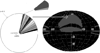
Figure 1: Sketch of the sample geometry. The whole sample has been divided into 12 slices ($\thickapprox$ 2.5 degrees each) in $\eta$.

There are two major reasons for choosing 12 slices: (1) each slice is approximately two-dimensional and (2) the slice-to-slice variations determine error bars, while keeping the number of objects per slice at a fairly high level. Each slice includes around 2977 galaxies and those galaxy positions are projected onto a two-dimensional image (projection perpendicular to the slice).

Mock samples from two model universe simulations were used to compare with the observational samples. One model universe is from the NYU Mock Galaxy Catalog (Berlind et al., 2006) in redshift (velocity) space, henceforth referred as NYUr. They used the Hashed-Oct-Tree (HOT) code (Warren & Salmon 1993) to make N-body simulations of the $\lambda$CDM cosmological model, with $\Omega_{m}=0.3,\Omega_{\lambda}=0.7,\Omega{b}=0.04,h=H_{0}/(100kms^{-1}Mpc^{-1})$ = 0.7, $n$ = 1.0, and $\sigma_{8}=0.9$. They identify halos in the dark matter particle distributions using a friends-of-friends algorithm with a linking length equal to 0.2 times the mean inter particle separation. They then populate these halos with galaxies using a simple model for the HOT of galaxies more luminous than a luminosity threshold. Every halo with a mass $M$ greater than a minimum mass $M_{min}$ gets a central galaxy that is placed at the halo center of mass and is given the mean halo velocity. A number of satellite galaxies is then drawn from a Poisson distribution with mean $<N_{sat}>=((M\cdot M_{min})/M_{1})^{\alpha}$, for $M\geq M_{min}$. These satellite galaxies are assigned the positions and velocities of randomly selected dark matter particles within the halo. This model is in good agreement with a wide variety of cosmological observations (see, e.g., Spergel et al. (2004); Seljak et al. (2005); Abazajian (2005)). Another mock sample is from the Millennium Run Semianalytic Galaxy Catalogue (Crotonet al., 2005) produced at the Max-Planck Institute for Astrophysics (MPA), henceforth referred to as MPAr. The simulation itself was carried out with a special version of the GADGET-2 code (Springel et al., 2001b, 2005). They use $\Omega_{m}=\Omega_{dm}+\Omega_{b}=0.3,\Omega_{b}=0.045,h=0.73,n=1.0$, and $\sigma_{8}=0.9$. They apply in post-processing an improved and extended version of the SUBFIND algorithm of (Springel et al., 2001a) to identify halos and a semianalytic model MODEL to build galaxies. A third mock sample is an entirely randomly distributed set of points. Fig. 2 shows examples of slices from each sample used in this paper.

Figure 2: Example observed and mock samples slices.

4 RESULTS AND DISCUSSION

Fig. 3 shows the calculated output functions (Section 2.1) for the observational SDSS data, as well as for all mock sample data, where only the functions corresponding to the size scale 15 Mpc (smoothed to that scale) are shown. The error bars are calculated from the variance of the results over 12 slices for each sample (every sample has the same geometry for the 12 slices). The $x$-axis represents the threshold value $\Sigma$, which is linearly distributed between the minimum ($\Sigma$=0) and maximum ($\Sigma$=10) pixel values for each smoothed slice.

Figure 3: Output functions from the MST for the size scale 15 Mpc: Distribution of components ($n$), density ($m$), filament ($f$), pixels ($j$), and volume ($v$). For uniform image, because there is only one value (the maximal pixel value equal with minimal value), no pixels can be found above any threshold value, $n$=0, $m$=0, $f$=0, j=0, and $v$=0 (straight thick solid line)

First we are interested to see how far the observed sample is from the uniform image at each scale, and we also want to see how different smoothing lengths influence the coordinates obtained from the comparison. Fig. 4 displays the changes with smoothing scale. We find there is an exponential change for all output functions.

Figure 4: Results of the observed sample compared with uniform image on different filtering scales. We calculate the distance between all samples and uniform images on every scale by Equation (8). The x-axis value is smoothing length and has ranges from 5 Mpc to 250 Mpc.

To quantify the differences between all the mock sample curves and the observational curves such as shown in Fig. 3, Equation (8) was used to calculate coordinates in metric space. Each coordinate gives quantitative information as to “how far” the mock sample is from the observed case. Coordinates were calculated for each output function, at each size scale. Table 1 shows the coordinates, where, for simplicity, the scale sizes were categorized into four groups (i.e., small, medium, large and huge scales). Also shown are the distance values obtained from the maximal coordinate ranking scheme (Section 2.2). Simply speaking, for each output function at each scale group we find the maximal value first (among observed, NYUr, MPAr and random samples), and then other values will be normalized by this maximal value (the maximal value itself will be changed to “1” after normalization). In this way we normalize the different output functions to sum them together. The resulting sum quantifies the overall differences between mock sample data and observational data at each scale. The lower the distance value, the closer the mock data is to the observed sample.

Table 1: MST Coordinates and Overall Distance Between Models and Observational Data

Filtering Scale	Sample	Components	Density	Filament	Pixels	Volume	Maximal Ranking
Small	NYUr	37.27	0.04	0.36	2611	0.003	0.75
(5–10mpc)	MPAr	62.99	0.03	0.41	3720	0.005	0.86
	Random	1230.98	0.38	0.69	48224	0.090	5
Medium	NYUr	4.05	0.04	0.18	8021	0.012	0.62
(15–30mpc)	MPAr	12.78	0.11	0.34	13879	0.026	1.28
	Random	77.77	0.82	0.45	94207	0.284	5
Large	NYUr	3.66	0.07	0.25	12174	0.024	0.78
(40–80mpc)	MPAr	5.71	0.17	0.33	17129	0.044	1.22
	Random	16.93	1.02	0.81	98539	0.341	5
Huge	NYUr	2.57	0.10	0.33	17950	0.035	0.97
(120–250mpc)	MPAr	2.81	0.24	0.47	24900	0.060	1.38
	Random	7.22	0.97	1.50	101196	0.320	5

Note. — The maximal coordinate ranking used to calculate the distance takes only the new definition of the filament output function.

Table 1 clearly shows how the random mock sample is systematically the farthest from the observational data. In order to get a better assessment of the more subtle differences from the other mock samples, the distance values between each mock sample and the observational data were plotted as a function of the size scale in Fig. 5, along with the rankings obtained from the individual output functions.

Figure 5: Metric distance (see Equation (8)) for maximal ranking result and output functions from mock samples. 1$\sigma$ error bars are shown. We also plot the straight thick solid line representing the zero value of distance from the observed sample.

We can see that on small scales, both mock samples are within 1$\sigma$ error bar range for the density, pixels and volume output function compared to the observations. We also note that the random sample has a consistently large metric distance from the observed sample and that NYUr is consistently and significantly closer to the observed sample case (zero values in Fig. 5) than the MPAr simulation results. To investigate the reason for the difference between the simulations, we repeated the above analysis, but using the mock samples in physical space (MPAp and NYUp — as opposed to redshift space MPAr and NYUr).

While it is technically inappropriate to compare our redshift space observation sample with galaxy distributions without velocity distortion, the results were informative. In Fig. 6 we see on small scales that even the random sample is more closely matched to the observed sample than NYUp and MPAp are. That is reasonable because the lack of redshift distortion significantly changes the structure on small scales. We also see in Fig. 6 that MPAp is closer to the observed sample statistics than NYUp in the maximal ranking method (as well as most of the individual output functions). Considering the opposite tendency for NYUr and MPAr, it is clear the two methods for assigning velocities to galaxies in the MPA and NYU simulations make a noticeable difference.

Figure 6: Metric distance (see Equation (8)) for maximal ranking result and output functions from mock samples in physical space.

5 CONCLUSION

We have used a slightly modified MST of Adams & Wiseman (1994) on multiple scale to study the morphology of galaxy distributions. The technique gives a detailed morphological description of galaxy distributions in metric space, on scales from about 5 Mpc to about 250 Mpc, with five output functions showing strong statistical differences. We also find that the filament output function values are high for the observations at small filtering scales but at around 50 Mpc the function approaches a lower stable value. Considering that most voids in SDSS galaxies are around 30–50 Mpc (Gott et al., 2005), this seems a likely signature of those voids.

The key motivation for this work is to supplement traditional tools with a more informative way of quantifying the similarity in the “visual” morphological properties between simulations and the observed universe. We use the “metric distance” as the parameter to describe that similarity through multiple measures by calculating the value of each of the MST output functions. We combine the values of each of the output functions into one “final” parameter for each simulation by the maximal ranking method. In Table 1 and Fig. 5, it was demonstrated that two N-body simulations have done a similar job of approximating our universe and that NYUr is more close to the observed sample than MPAr. From the analysis for Fig. 6, we surprisingly found that MPAp is more closely matched than the NYUp to the observed sample in redshift space, with the implication that velocity determinations for simulation galaxies is a major contributor to the relatively poorer match of the MPA simulation. The velocities of satellite galaxies in NYU simulation halos are assigned randomly from the dark matter particles within the haloes (Berlind et al., 2006). However, in the MPA simulation, even satellite galaxies have interpolated velocities (taken from the subhalo) rather than just randomly assigned ones (Croton, 2008). It is very likely that the mechanism for producing the velocity of satellite galaxies in MPA simulation contributes noticeably to the relative shortcomings of MPAr in Fig. 5.

While the MST yields a single statistic for comparison of structure maps, in a way similar to other measures of large scale structure, we submit that its greater utility is in providing multiple intermediate outputs that convey insight into the physical differences between samples that lead to the statistical result. Of the many topological characteristics, threshold values, and scale samplings that the MST aggregates into a final result, we highlight a few examples of the specific physical differences that the technique reveals.

First, we have the expected result that the random sample is much different from all other samples at virtually all scales for all output functions. We have chosen only to use that case for normalization in the maximal ranking step.

Now, for our much more meaningful comparisons among MPA, NYU, and observed samples, we see that for the density output function, MPA has more high-density pixels (at about the 5$\sigma$ level) than NYU sample, and the NYU sample has more high-density pixels than observed sample (1-2 $\sigma$). The volume and pixels output functions show similar trends as the density output function with the implication that those high-density pixels are also accompanied by large area regions of pixels above the various thresholds. The components and filament output functions are more complicated and fluctuate with the increasing scale. Simply speaking, for scales less than 50 Mpc, NYU and the observed sample are close to each other (around 1 $\sigma$), but MPA clearly has many more sizeable clumps (greater than 3$\sigma$) and is also more filamentary (greater than 3$\sigma$). For scales more than 50 Mpc, MPA shows more filamentary structure (greater than 3$\sigma$) than NYU sample, which is a little more filamentary (0.5-2 $\sigma$) than the observed sample. And observed sample has more clumps (1$\sigma$) than both mock samples.

Our next step is to apply the MST to the full three-dimensional galaxy distribution, which will require redevelopment/extension of output functions.

Appendix A Generalizing the Filament Index Definition

Let us first recall the definition of the filament index:

$$F={\pi D^{2}\over{4A}}.$$ (A1)

Note first that $F$ depends only upon two values, $D$ and $A$, which are respectively the diameter and the area of the component. Since we use the standard definition of a diameter (i.e., for a component $S$, the diameter of $S$ is $D(S)=\max_{x,y\in S}\{|x-y|\}$), there is a possibility that two components having quite different structures end up having the same filament index value (Fig. 7).

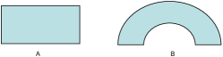
Figure 7: $A$ and $B$ have the same diameter and the same area and therefore, the same filament index, even though their structure is quite different.

The diameter, and therefore the filament index of non-convex components is under-estimated. Contrary to what was originally said in Khalil et al. (2004), the cause of this problem is not the fact that the definition of the diameter is not well adapted for non-convex components. A closer look at the definition of the filament index shows that one of its attributes is the circumference of a circle, $P_{\circ}=\pi D$:

$$F={\pi D^{2}\over{4A}}={(\pi D)D\over{4A}}={P_{\circ}D\over{4A}}.$$ (A2)

So by definition, the filament index “expects” to be treating convex objects (a circle certainly being the most trivial example of a convex object). And that is where the change should be made: Instead of changing the definition of the diameter, one should simply change the definition of the perimeter to have it in its most general form, $P$. So the generalized version of the filament index is therefore

$$F={PD\over{4A}},$$ (A3)

where $P$ is the perimeter of the underlying object.

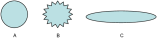
Figure 8: Objects $A$, $B$, and $C$ in order of increasing filament index value. All have the same area. $A$ and $B$ have the same diameter, but since the perimeter of $B$ is larger, their (newly generalized) filament index is different. Since object $C$ has a larger diameter and a larger perimeter than object $A$, it therefore has a larger filament index. And although objects $B$ and $C$ have the same perimeter, since object $C$ has a larger diameter, it has a larger filament index.

One can readily see from Fig. 7 that although both objects have the same diameter and area, since their perimeter is quite different, object B will have the larger filament index, which is what one would intuitively expect. In Fig. 8 are shown three objects of increasing filament index value. One can easily see how the newly generalized filament index definition will greatly help in the distinction of different geometrical features in the analyzed objects (or components). However, this new definition of $F$ is still degenerate in the sense that one can still find an infinite number of objects having the same $F$. However, the degree of degeneracy is much less than for the standard, original definition of $F$.

References

- Abazajian (2005) Abazajian, K., Kadota, K., & Stewart, E. D. 2005, JCAP, 0508, 008
- Adams (1992) Adams, F. C. 1992, ApJ, 387, 572
- Adams & Wiseman (1994) Adams, F. C. & Wiseman, J. 1994, ApJ, 435, 693
- Adelman-McCarthy et al. (2007) Adelman-McCarthy, J. K., et al. 2007, ApJS, 172, 634
- Berlind et al. (2006) Berlind, A. A., et al. 2006, ApJS, 167, 1
- Blanton et al. (2005) Blanton, M. R., et al. 2005, AJ, 129, 2562
- Coles & Lucchin (1995) Coles, P. & Lucchin, F. 1995, Cosmology: The Formation and Evolution of Cosmic Structure (NY:Wiley)
- Crotonet al. (2005) Croton, D. J., et al. 2006, MNRAS, 365, 11
- Croton (2008) Croton, D. J. 2008, private communication.
- Dolag et al. (2008) Dolag, K., Borgani, S., Schindler, S., Diaferio, A., & Bykov, A. M. Space Sci.Rev., 134, 229
- Donoho (1988) Donoho, D. L. 1988, Ann. Stat., 16, 1390
- Gill et al. (2004) Gill, S. P. D., Knebe, A., & Gibson, B. K. 2004, MNRAS, 351, 399
- Gott et al. (2005) Gott, J. R., Jurić, M., Schlegel, D., Hoyle, F., Vogeley, M., Tegmark, M., Bahcall, N., & Brinkmann, J. 2005, ApJ624, 463
- Khalil (2004) Khalil, A. 2004, PhD thesis, Univ. Laval (available online at http://www.theses.ulaval.ca/2004/22165/22165.pdf)
- Khalil et al. (2004) Khalil, A., Joncas, G., & Nekka, F. 2004, ApJ, 601, 352
- Khalil et al. (2006) Khalil, A., Joncas, G., Nekka, F., Kestener, P., & Arneodo, A. 2006, ApJS, 165, 512
- Kiang, Wu & Zhu (2004) Kiang, T., Wu, Y., & Zhu, X. 2004, Chin. J. Astron. Astrophys., 3, 209
- Martinez et al. (2005) Martinez, V. J., Starck, J. L., Saar, E., Donoho, D. L., Reynolds, S., Cruz .P., & Paredes, S. 2005, ApJ, 634, 744
- Peebles (1980) Peebles, P.J.E. 1980, Principles of Physical Cosmology, Princeton University Press
- Saar et al. (2007) Saar E., Martinez V.J., Starck J.-L., Donoho D.L. 2007, MNRAS, 374, 1030
- Sahni et al. (1997) Sahni, V., Sathyaprakash, B.S., & Shandarin, S.F. 1997, ApJ, 476, L1
- Seljak et al. (2005) Seljak, U., et al. 2005, Phys. Rev. D71, 103515
- Shandarin (1983) Shandarin, S.F. 1983, Soviet Astron. Lett., 9, 104
- Silverman (1981) Silverman, B. W. 1981, J. R. Stat. Soc. B, 43, 97
- Skrutskie et al. (2000) Skrutskie, M. F., et al. 2006, AJ, 131, 1163
- Spergel et al. (2004) Spergel, D. N., et al. 2004, ApJ, 608, 10
- Springel et al. (2005) Springel, D. N., et al. 2005, Nature, 435, 629
- Springel et al. (2005) Springel, D. N., et al. 2005, MNRAS, 364, 1105
- Springel et al. (2001a) Springel V., White S. D. M., Tormen G., Kauffmann G., 2001a, MNRAS, 328, 726
- Springel et al. (2001b) Springel V., Yoshida N., White S. D. M., 2001b, New Astron., 6, 79
- Taylor et al. (2003) Taylor, A. R., et al. 2003, AJ, 125, 3145
- Warren & Salmon (1993) Warren M.S., Salmon J.K., A parallel hashed oct-tree N-body algorithm. In Supercomputing ’93, pages 12-21, Los Alamitos, 1993. IEEE Comp. Soc.
- Weinberg (2005) Weinberg, D. H. 2005, Science, 309, 564
- White (1979) White S.D.M. 1979, MNRAS186,145
- Wiseman & Adams (1994) Wiseman, J. & Adams, F.C. 1994, ApJ, 435, 708
- Wu, Batuski & Khalil (2008) Wu, Y., Batuski, D. J., & Khalil, A. 2008, The Fractal Structure of the Universe (Germany :VDM Verlag Dr. Mueller e.K.)
- York et al. (2000) York, D. G., et al. 2000, AJ, 120, 1579
- Zeldovich (1982) Zeldovich, Ya. B. 1982, Soviet Astron. Lett., 8, 102