Dynamics of a double pendulum with distributed mass

Abstract

We investigate a variation of the simple double pendulum in which the two point masses are replaced by square plates. The double square pendulum exhibits richer behavior than the simple double pendulum and provides a convenient demonstration of nonlinear dynamics and chaos. It is also an example of an asymmetric compound double pendulum, which has not been studied in detail. We obtain the equilibrium configurations and normal modes of oscillation and derive the equations of motion, which are solved numerically to produce Poincaré sections. We show how the behavior varies from regular motion at low energies, to chaos at intermediate energies, and back to regular motion at high energies. We also show that the onset of chaos occurs at a significantly lower energy than for the simple double pendulum.

I Introduction

The simple double pendulum consisting of two point masses attached by massless rods and free to rotate in a plane is one of the simplest dynamical systems to exhibit chaos.richter84 ; korsch99 ; stachowiak06 It is also a prototypical system for demonstrating the Lagrangian and Hamiltonian approaches to dynamics and the machinery of nonlinear dynamics.landau76 ; goldstein80 ; kibble05 ; gregory06 Variants of the simple double pendulum have been considered, including an asymmetrical version,newton89 and a configuration in which the inner mass is displaced along the rod.levien93 The compound (distributed-mass) double pendulum is a generalization that is easier to implement as a demonstration. For example, the double bar pendulum in which the point masses are replaced by slender bars has been the subject of a number of studies,shinbrot92 ; zhou96 ; ohlhoff00 and a version of the double square pendulum is available commercially.chaoticpendulums The dynamics of the general symmetrical compound double pendulum has also been investigated, including a proof that it is a chaotic system.dullin94

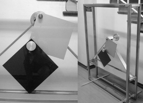
Fig. 1: The double square pendulum in the School of Physics at the University of Sydney. Left: close up of the two plates. Right: the pendulum and its enclosure.

The School of Physics at the University of Sydney has a large-scale variation of the compound planar double pendulum (see Fig. 1). The double square pendulum consists of two square metal plates connected together by two axles. It is set into motion by rotating a wheel at the back, which is attached to the axle on the inner plate. The axles are housed in low friction bearings, so that when the wheel is turned and released, the plates continue in a complex motion that lasts several minutes.wheatland08a The demonstration is housed inside a large glass and metal enclosure measuring about 120 cm by 120 cm by 25 cm, and the square metal plates are approximately 28 cm on a side. The double square pendulum is located in the main corridor of the building and attracts considerable attention from passing students. The School also has a smaller, bench-mounted version of the double square pendulum, suitable for classroom demonstrations.

The double square pendulum exhibits diverse and at times unpredictable behavior. For small pushes on the driving wheel, the system oscillates back and forth about the equilibrium position shown in Fig. 1. If the driving wheel is rotated very rapidly, the inner plate spins rapidly and throws the other plate outward, and the motion is again fairly regular. For intermediate rates of rotation of the driving wheel the system exhibits unpredictable motions.

This general behavior is similar to that of the simple and compound planar double pendula.korsch99 ; ohlhoff00 However, the double square pendulum described here differs from previously studied systems. It is a compound pendulum, but the center of mass of the inner plate does not lie along the line joining the two axles. In this regard it is closest to the asymmetrical double pendulum studied in Ref. newton89, , although that pendulum does not have distributed mass. The dynamics of the double square pendulum is interesting both from the viewpoint of elucidating the physics of a classroom physics demonstration and as a pedagogical exercise illustrating the application of dynamical theory.

In this paper we investigate an idealized model of the double square pendulum. We first obtain the equations of motion using the Lagrangian formalism (Sec. II). General statements are then made about the basic motion of the double pendulum: the energy ranges for different types of motion of the pendulum are identified, and the behavior at low energy (Sec. III.1) and at high energy (Sec. III.2) is described. The equations of motion are expressed in dimensionless form in Sec. IV and solved numerically to produce Poincaré sections of the phase space of the pendulum, which are constructed at increasing values of the total energy in Sec. V. Section VI includes a brief qualitative comparison with the real double square pendulum.

II Equations of motion

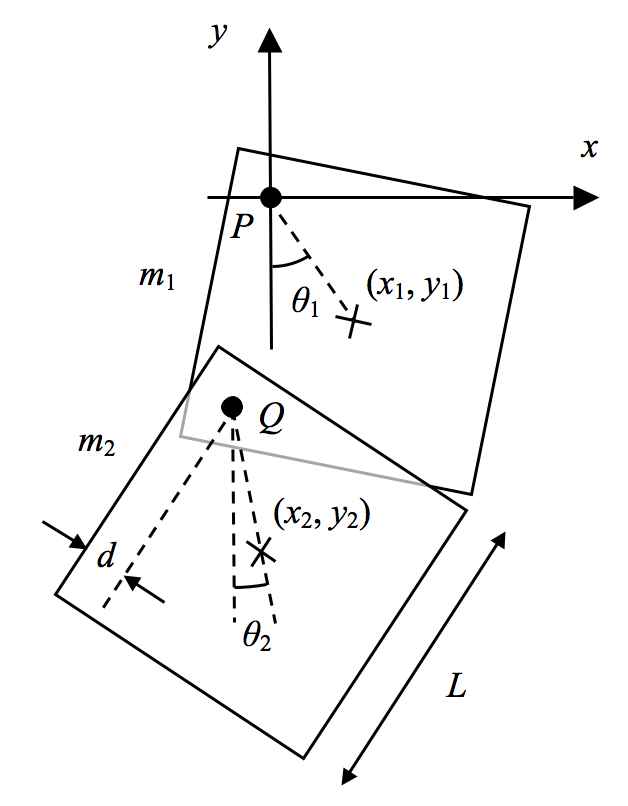
Fig. 2: A model of the double square pendulum.

Consider a double pendulum comprising two square plates with side length $L$ and masses $m_{1}$ and $m_{2}$ (see Fig. 2). The inner plate rotates about a fixed axle at $P$ and the outer plate rotates about an axle fixed to the inner plate at $Q$. We neglect the effect of friction at the axles. The plates are assumed to have uniform mass densities and the axles are assumed to be massless, so that the center of mass of each plate is at its center. A coordinate system with origin at $P$ is defined as shown and the center of mass of the inner and outer plates are located at positions $(x_{1},y_{1})$ and $(x_{2},y_{2})$, respectively. The center of mass of the plates subtend angles $\theta_{1}$ and $\theta_{2}$ with respect to the direction of the negative $y$ axis.

The double square pendulum shown in Fig. 1 has relatively large axles, and in particular the central axle has a wheel attached to it. The presence of massive axles changes the locations of the center of mass of each plate. However, the simple model considered here is expected to capture the essential dynamics of the real double square pendulum.

The equations of motion of the model pendulum may be derived using Lagrangian dynamics.landau76 ; goldstein80 ; kibble05 ; gregory06 The Lagrangian is $\mathcal{L}=T-V$, where $T$ is the kinetic energy and $V$ is the potential energy of the pendulum. The kinetic energy is the sum of the kinetic energies of the center of mass of the two plates, each of which has a linear and a rotational component:

$$T=\frac{1}{2}m_{1}(\dot{x}_{1}^{2}+\dot{y}_{1}^{2})+\frac{1}{2}I_{1}\dot{\theta}_{1}^{2}+\frac{1}{2}m_{2}(\dot{x}_{2}^{2}+\dot{y}_{2}^{2})+\frac{1}{2}I_{2}\dot{\theta}_{2}^{2},$$ (1)

where $I_{1}$ and $I_{2}$ are the moments of inertia about the center of mass, and are given by $I_{i}=\frac{1}{6}m_{i}L^{2}$ for $i=1,2$. The potential energy is the sum of the potential energy of each plate, and is given by

$$V=m_{1}gy_{1}+m_{2}gy_{2}+V_{0},$$ (2)

where $V_{0}$ is a suitable reference potential.

If we express $y_{1}$ and $y_{2}$ in terms of $\theta_{1}$ and $\theta_{2}$, we obtain

$$V=-2m_{2}k_{1}\left[\cos(\theta_{1}-\alpha)+\sin\alpha\cos\theta_{2}\right]+V_{0},$$ (3)

where

$$\alpha=\tan^{-1}\frac{m_{2}}{m_{1}+m_{2}},$$ (4)

and

$$k_{1}=\frac{\sqrt{2}g\ell}{4}\mathrm{cosec}\,\alpha,$$ (5)

with $\ell=L-2d$.

Equilibrium configurations of the pendulum occur when $V=V(\theta_{1},\theta_{2})$ is stationary with respect to $\theta_{1}$ and $\theta_{2}$. The four equilibrium configurations are

$$(\theta_{1},\theta_{2})=(\alpha,0),\quad(\alpha,\pi),\quad(\alpha+\pi,0),\quad\textrm{and}\quad(\alpha+\pi,\pi);$$ (6)

but $(\theta_{1},\theta_{2})=(\alpha,0)$ is the only stable equilibrium. The equilibrium configurations are illustrated in Fig. 3 with the stable equilibrium at the upper left. The angle $\alpha$, defined by Eq. (4), is the angle that the center of mass of the inner plate makes with the negative $y$ axis in stable equilibrium.

It is convenient to choose $V_{0}$ so that the potential energy of the pendulum is zero in stable equilibrium. In this case the potential energies of the pendulum in the three unstable equilibrium configurations are $V=E_{i}$ (with $i=1,\,2,\,3$), where

$$E_{1} = \sqrt{2}m_{2}g\ell,$$ (7a)

$$E_{2} = E_{1}\,\mathrm{cosec}\,\alpha,$$ (7b)

$$E_{3} = E_{1}+E_{2}.$$ (7c)

The configurations shown in Fig. 3 are labeled by these energies.

It is convenient to remove the dependence of the equilibrium coordinates on $\alpha$ by introducing the change of coordinates

$$\varphi_{1}=\theta_{1}-\alpha\quad\textrm{and}\quad\varphi_{2}=\theta_{2}.$$ (8)

With these choices the potential energy of the pendulum may be written as

$$V=\frac{1}{2}\left[(1-\cos\varphi_{1})E_{1}+(1-\cos\varphi_{2})E_{2}\right].$$ (9)

The simple double pendulum has analogous equilibrium configurations, and its potential energy may also be expressed in the form of Eq. (9).korsch99

In terms of the coordinates in Eq. (8) the kinetic energy of the pendulum in Eq. (1) may be written as

$$T=m_{2}(k_{2}{\dot{\varphi}_{1}}^{2}+2k_{3}\dot{\varphi}_{1}\dot{\varphi}_{2}\sin\beta+k_{4}\dot{\varphi}_{2}^{2}),$$ (10)

where

$$k_{2} =\frac{1}{12}\left[(m_{1}/m_{2})L^{2}+3(m_{1}/m_{2}+2)\ell^{2}\right],$$ (11)

$$k_{3} =\sqrt{2}\ell^{2}/4,\qquad k_{4}=\frac{1}{12}(L^{2}+3\ell^{2}),$$ (12)

and

$$\beta=\pi/4+\alpha+\varphi_{1}-\varphi_{2}.$$ (13)

We apply the Euler-Lagrange equationslandau76 ; goldstein80 to the Lagrangian $\mathcal{L}=T-V$ given by Eqs. (9) and (10) and obtain the equations of motion:

$$k_{2}\ddot{\varphi}_{1}+k_{3}(\ddot{\varphi}_{2}\sin\beta-\dot{\varphi}_{2}^{2}\cos\beta)+k_{1}\sin\varphi_{1} = 0,$$ (14a)

$$k_{4}\ddot{\varphi_{2}}+k_{3}(\ddot{\varphi}_{1}\sin\beta+\dot{\varphi}_{1}^{2}\cos\beta)+k_{5}\sin\varphi_{2} = 0,$$ (14b)

where

$$k_{5}=\sqrt{2}g\ell/4.$$ (15)

III General Features of the Motion

The coupled, nonlinear equations of motion in (14) are not amenable to analytic solution, and it is necessary to solve these equations numerically to investigate the motion. Some general statements can be made about the behavior for a given energy, and about the nature of the motion at small and large energies.

The motion of the pendulum depends on its total energy $E=T+V$. The magnitude of the energy in relation to the three energies $E_{1}$, $E_{2}$, and $E_{3}$ specified by Eq. (7) determines whether the plates of the pendulum can perform complete rotations. For $E\leq E_{1}$ each of the plates may oscillate about stable equilibrium, but there is insufficient energy for either plate to perform a complete rotation. For $E_{1}<E\leq E_{2}$ the energy of the pendulum is sufficient to allow complete rotation of the outer plate about the axle at $Q$ (see Fig. 2), but rotational motion of the inner plate is still prohibited. One or other of the plates may rotate for $E_{2}<E\leq E_{3}$, and simultaneous rotation becomes possible when $E>E_{3}$. The simple double pendulum has analogous behavior.korsch99

III.1 Motion at low energy

The nonlinear terms in the equations of motion have negligible influence when the total energy is small, in which case the pendulum oscillates with small amplitude about stable equilibrium. In this regime the equations may be simplified by using small-angle approximations and dropping nonlinear terms,hand98 ; kibble05 ; gregory06 leading to the linear equations:

$$k_{2}\ddot{\varphi}_{1}+k_{6}\ddot{\varphi}_{2}+k_{1}\varphi_{1} =0,$$ (16a)

$$k_{4}\ddot{\varphi}_{2}+k_{6}\ddot{\varphi}_{1}+k_{5}\varphi_{2} =0,$$ (16b)

where

$$k_{6}=k_{3}(\cos\alpha+\sin\alpha)/\sqrt{2}.$$ (17)

These equations have the general form expected for coupled linear oscillators.main84

Normal modes of oscillation are motions of the pendulum in which the coordinates $\varphi_{1}$ and $\varphi_{2}$ vary harmonically in time with the same frequency and phase, but not necessarily with the same amplitude.gregory06 The substitution of harmonic solutions into the linearized equations of motion (16) leads to the identification of two normal frequencies $\omega_{+}$ and $\omega_{-}$, corresponding to fast and slow modes of oscillation:

$$\omega_{\pm}^{2}=\frac{k_{1}k_{4}+k_{2}k_{5}\pm\sqrt{(k_{1}k_{4}-k_{2}k_{5})^{2}+2k_{1}k_{5}k_{6}^{2}}}{2a},$$ (18)

where $a=k_{2}k_{4}-k_{6}^{2}$. The amplitude factors $A_{1}$ and $A_{2}$ for the harmonic motions of the two coordinates are related by

$$\Big{(}\frac{A_{1}}{A_{2}}\Big{)}_{\pm}=\frac{-k_{5}k_{6}}{a\omega_{\pm}^{2}-k_{1}k_{4}}.$$ (19)

For the slow mode $(A_{1}/A_{2})_{+}>0$, so that the plates oscillate in the same direction; for the fast mode $(A_{1}/A_{2})_{-}<0$, and the plates oscillate in opposite directions.

A simple case considered in Secs. IV and V occurs when $m_{1}=m_{2}$ and $\ell=L$; that is, the plates have equal mass and the axles are located at the corners of the plates. In that case the normal frequencies are $\omega_{+}\approx 1.66(g/L)^{1/2}$ and $\omega_{-}\approx 0.782(g/L)^{1/2}$, and the amplitudes are $A_{1}\approx-0.613A_{2}$ for the fast mode and $A_{1}\approx 0.730A_{2}$ for the slow mode.

The general motion at low energy may be expressed as linear combinations of the normal modes,main84 in which case the motion is no longer periodic, but is quasi-periodic. The motion never quite repeats itself for general initial conditions. The simple double pendulum has analogous behavior at low energy.korsch99

III.2 Motion at high energies

At high energy the pendulum behaves like a simple rotor, with the system rotating rapidly in a stretched configuration ($\theta_{1}\approx\pi/4$, $\theta_{2}\approx 0$). In this case the kinetic energy terms in the Lagrangian dominate the potential energy terms and may be described by setting $g=0$ in the equations of motion. The total angular momentum is conserved, because in the absence of gravity, there is no torque on the pendulum. The resulting motion of the system is regular (non-chaotic), because a system with two degrees of freedom and two constraints (conservation of total energy and total angular momentum) cannot exhibit chaos.richter84 It follows, for example, that the double square pendulum would not exhibit chaos if installed on the space station. The simple double pendulum has analogous behavior.korsch99

IV Numerical Methods

To investigate the detailed dynamics of the pendulum the equations of motion are solved numerically by using the fourth-order Runge-Kutta method.press92 The accuracy of the integration may be checked by evaluating the energy of the pendulum at each integration step. If there is a discrepancy between the calculated energy and the initial energy of the pendulum, the integration step may be modified accordingly.

The equations of motion of the pendulum may be written in dimensionless form by introducing

$$\overline{t}=\sqrt{\frac{g}{L}}t,\quad\overline{L}=\frac{\ell}{L},\quad\text{and}\quad\overline{m}=\frac{m_{1}}{m_{2}}.$$ (20)

An appropriate dimensionless energy is

$$\overline{E}=\frac{E}{\frac{1}{12}m_{2}gL}.$$ (21)

In Sec. V the system is simplified by considering equal mass plates and by locating the axles at the corners of the plates. These choices imply parameter values

$$\overline{L}=1\quad\text{and}\quad\overline{m}=1.$$ (22)

With these choices, the energies of the pendulum corresponding to Eq. (7) are $\overline{E}_{1}\approx 16.97$, $\overline{E}_{2}\approx 37.95$, and $\overline{E}_{3}\approx 54.92$. In Sec. V we also use dimensionless variables and drop the bars for simplicity.

V General Dynamics and Poincaré Sections

The general dynamics of the pendulum may be investigated by analyzing the phase space for increasing values of the total energy. The phase space of the pendulum is three-dimensional. (There are four coordinates, that is, $\varphi_{1}$, $\varphi_{2}$, $\dot{\varphi}_{1}$, and $\dot{\varphi}_{2}$, but one of these may be eliminated because energy is conserved.) The phase space can be examined by considering the two-dimensional Poincaré section,drazin92 ; korsch99 ; hilborn00 defined by selecting one of the phase elements and plotting the values of others every time the selected element has a certain value. For a given choice of initial conditions the Poincaré section shows points representing the intersection of an orbit in phase space with a plane in the phase space. Periodic orbits produce a finite set of points in the Poincaré section, quasi-periodic orbits produce a continuous curve, and chaotic orbits result in a scattering of points within an energetically accessible region.drazin92 ; korsch99

V.1 Defining a Poincaré section

We use conservation of energy to eliminate $\dot{\varphi}_{2}$ and choose the Poincaré plane to be $\varphi_{2}=0$. A point $(\varphi_{1},\dot{\varphi}_{1})$ is recorded in the phase space of the inner plate whenever the outer plate passes through the vertical position $\varphi_{2}=\theta_{2}=0$. When this condition occurs, the outer plate may have positive or negative momentum. To ensure a unique definition of the Poincaré section a point is recorded if the outer plate has positive momentum; that is, a point is recorded in the phase space of the inner plate whenever

$$\varphi_{2}=0\qquad\textrm{and}\qquad{p}_{2}>0,$$ (23)

where $p_{2}=\partial{\mathcal{L}}/\partial\dot{\varphi}_{2}=6\sqrt{2}\dot{\varphi}_{1}\sin\beta+8\dot{\varphi}_{2}$ is the generalized momentum corresponding to $\varphi_{2}$. In the following we present Poincaré sections as plots of $\dot{\theta}_{1}$ versus $\theta_{1}$, with the angles in degrees.

V.2 Results

Figure 4 shows the results of constructing Poincaré sections for values of the total (dimensionless) energy ranging from $E=0.01$ to $E=2\times 10^{4}$.wheatland08b Each section was constructed by numerically solving Eq. (16) at a given energy for many different initial conditions; 40–60 initial conditions were used for the cases shown in Fig. 4, with initial conditions chosen to provide a good coverage of the energetically accessible region in the plane.

For energy $E=0.01$ [Fig. 4(a)] the Poincaré section is covered by two regions of stable elliptical orbits around two fixed points located on the line $\theta_{1}=\alpha\approx 26.6^{\circ}$, and this entire section has approximate reflection symmetry about this line. The motion of the pendulum is regular (that is, periodic and quasi-periodic) at low values of its total energy. The fixed points correspond to the two strictly periodic normal modes identified in Sec. III.1, with the upper fixed point corresponding to the co-oscillating slow mode, and the lower fixed point corresponding to the counter-oscillating fast mode. The behavior observed in Fig. 4(a) corresponds to the solution of the linearized equations of motion in Eq. (16), and is strictly regular. The horizontal and vertical extent of the section is very small (a few degrees) due to the small energy.

Figure 4(b) shows the Poincaré section for $E=0.65$. The section has lost the reflection symmetry about $\theta_{1}=\alpha\approx 26.6^{\circ}$ observed in Fig. 4(a). This loss of symmetry is related to the non-symmetrical geometry of the pendulum (the center of mass of the inner plate is offset to the right). The section is much larger, spanning almost $30^{\circ}$ in $\theta_{1}$, and almost $40^{\circ}$ in $\dot{\theta}_{1}$ (recall that time is dimensionless), due to the larger energy. A striking feature of this section is that the lower fixed point has undergone a period-doubling bifurcation, resulting in a pair of stability islands separated by a separatrix within the lower stability region. A trajectory producing an orbit in either of these stability islands produces a corresponding orbit in the other due to the period $2$ nature of the orbit.

The first signs of chaotic behavior appear at $E\approx 4$–4.5 [see Fig. 4(c) for $E=4.5$] in the form of a scattering of points around the hyperbolic point that sits between the four stability regions. The chaotic region first appears along the trajectory containing the hyperbolic point. As the energy is increased from $E=4.5$ to $E=8$ [Fig. 4(d)] the size of the chaotic region increases with the loss of regular orbits, particularly in the stability regions located at the upper left and upper right of the Poincaré section. The lower stability region remains unaffected.

The growth of chaos with energy is demonstrated by the next three Poincaré sections, corresponding to $E=E_{1}=16.97$ [Fig. 4(e)], $E=20$ [Fig. 4(f)], and $E=E_{2}=37.95$ [Fig. 4(g)]. Figure 4(e) corresponds to the pendulum having sufficient energy for the outer plate to rotate. It is striking that the Poincaré section has few regions with stable orbits, so that the pendulum is chaotic even at this modest energy. At $E=20$ [Fig. 4(f)] most of the invariant orbits in the upper stability region have been lost. Notably the upper fixed point persists, and is surrounded by small regions of stability. The upper fixed point corresponds to a large amplitude analog of the slow normal mode. Global chaos is achieved at energy $E\approx 25$ (not shown) where a single trajectory covers the entire Poincaré section and the system is completely ergodic. Note that this energy is less than $E_{2}=37.95$, the energy required for the inner plate to rotate. Hence completely chaotic behavior is achieved even without the rotation of the inner plate. Global chaos remains up to $E\approx 37$ at which energy a small stability island appears in the lower part of the Poincaré section and grows with energy. Figure 4(g) shows $E=E_{2}=37.95$. The Poincaré section has grown to a width of $360^{\circ}$ in $\theta_{1}$.

A second stability island appears near the upper part of the Poincaré section at $E\approx 75$. This stability island corresponds to quasi-periodic rotational motion of the entire pendulum, and is an very large amplitude analog of the slow normal mode. The two stability islands, plus a third stability island located on the left and right hand edges, are shown in the Poincaré section at $E=80$ [Fig. 4(i)].

The sizes of the stability regions increase with energy, as shown by the cases $E=150$ [Fig. 4(j)] and $E=500$ [Fig. 4(k)]. The motion of the pendulum becomes regular at very high values of $E$, as shown in Fig. 4(l), corresponding to $E=2\times 10^{4}$. The appearance of regular behavior at high energies was discussed in Sec. III.2, and explained in terms of the total angular momentum being conserved during the motion, in addition to the total energy. The section also becomes approximately reflection symmetric at this energy, about the line $\theta_{1}=45^{\circ}$.

V.3 Comparison with simple double pendulum

The geometry of the Poincaré sections presented in Sec. V.2 show some differences from those of the simple double pendulum and double bar pendulum.korsch99 ; ohlhoff00 ; richter84 ; stachowiak06 To better illustrate the differences we have numerically solved the equations of motion for the simple double pendulum, and constructed Poincaré sections using the definition given in Sec. V.1. For simplicity we consider a simple double pendulum with equal masses $M$, connected by massless rods with equal length $h$. The energy of the system is given in terms of $\frac{1}{12}Mgh$, and time is in terms of $\sqrt{h/g}$. The dimensionless energies corresponding to threshold values for complete rotation of the inner mass, outer mass, and both masses are $E_{1,\rm s}=24$, $E_{2,\rm s}=48$, and $E_{3,\rm s}=72$ respectively, where the subscript $s$ denotes the simple double pendulum. The energies are equally spaced due to the symmetry of the pendulum.

Figure 5 illustrates a sequence of Poincaré sections for the simple double pendulum, which may be considered to be comparable to certain sections shown in Fig. 4 for the double square pendulum, as described in the following.

At $E=0.01$ [Fig. 5(a)] the Poincaré section is very similar to that obtained for the double square pendulum at the same energy [Fig. 4(a)], except that the section for the simple double pendulum is symmetric about $\theta_{1}=0$ rather than $\theta_{1}=\alpha$, and the orbits in the section have exact reflection symmetry about this line (rather than approximate symmetry). All of the Poincaré sections for the simple double pendulum have strict reflection symmetry about $\theta_{1}=0$. In common with the double square pendulum the section at the lowest energy consists of regular orbits about two fixed points corresponding to two normal modes.

At somewhat higher energies [Fig. 5(b)] the orbits in the Poincaré section distort. Figure 5(b) is comparable to Fig. 4(b) with two notable differences. The Poincaré section for the double square pendulum exhibits period-doubling of the lower fixed point, which has no counterpart for the simple double pendulum (or for the double bar pendulum),korsch99 ; ohlhoff00 ; richter84 ; stachowiak06 and may be related to the non-symmetrical geometry of the double square pendulum. The other obvious difference is the loss of symmetry in the section for the double square pendulum.

Figure 5(c) illustrates the first appearance of chaos in the simple double pendulum; this section may be considered to be comparable to Fig. 4(c). Note that the double square pendulum first becomes chaotic at an energy substantially lower than that for the simple double pendulum in comparison to the respective threshold energies required for complete rotation of the masses. For the double square pendulum chaos appears at an energy $E_{\rm c}\approx 4$, a fraction $E_{\rm c}/E_{1}\approx 0.24$ of the energy required for the outer plate to rotate, and a fraction $E_{\rm c}/E_{3}\approx 0.07$ of the energy required for both plates to rotate. In comparison, chaos first appears in the simple double pendulum at $E_{\rm c,s}\approx 10$, which corresponds to $E_{\rm c,s}/E_{1,\rm s}\approx 0.42$ and $E_{\rm c,s}/E_{3,\rm s}\approx 0.14$ of the energy required for rotation of the outer mass and of both masses, respectively. This difference may be due to the additional complexity introduced into the motion by the geometrical asymmetry. Figures 5(c) ($E=10$) and 5(d) ($E=15$) illustrate the development of chaos, and are comparable to Figs. 4(c) and 4(d).

Figure 5(e) shows the Poincaré section for $E=32$; this section is comparable with Fig. 4(f). In both cases the pendula have sufficient energy for the lower mass, but not the upper mass, to rotate. Both Poincaré sections are chaotic, apart from stable regions around the upper fixed point, which corresponds to a large amplitude slow mode.

The geometry of the Poincaré section at very high energy ($E=2\times 10^{4}$) shown in Fig. 5(f) is very similar to that of the double square pendulum at the same energy [Fig. 4(l)]. This similarity is expected because at high energies the different pendula perform rotational motion in a stretched configuration, and the difference in geometry is of little importance. The section for the simple double pendulum is exactly symmetrical about $\theta_{1}=0$, whereas the section for the double square pendulum is approximately symmetrical about $\theta_{1}=45^{\circ}$.

VI Qualitative comparison with a real double square pendulum

A detailed comparison with a real double square pendulum requires an experimental investigation and solution of the equations of motion including the more complicated distributions of masses in that double square pendulum, which is beyond the scope of this article. In this section we make some brief qualitative comparisons between the results of the model and the behavior of the double square pendulum.

As mentioned in Sec. I, the real double square pendulum exhibits regular behavior at high and low energies and irregular behavior at intermediate energies. One way to demonstrate the range of behavior of a real double square pendulum is to set it into motion with high energy, and to watch the change in behavior as the double square pendulum slowly loses energy due to friction.

It is straightforward to demonstrate each of the normal modes in a real double square pendulum by turning the central wheel back and forth with small amplitude and with the appropriate frequencies. By timing multiple oscillations, the periods of the normal modes were measured to be $T_{+}\approx 0.70\pm 0.01\,{\rm s}$ and $T_{-}\approx 1.23\pm 0.01\,{\rm s}$. For equal mass plates with axles at the corners of the plates ($\ell=L$), and $L=0.28\,{\rm m}$ and $g=9.81\,{\rm m}\,{\rm s}^{-2}$, Eq. (18) predicts $T_{+}\approx 0.64\,{\rm s}$ and $T_{-}\approx 1.36\,{\rm s}$. If we include an offset of the axles ($\ell=0.1L$), the result is $T_{+}\approx 0.64\,{\rm s}$ and $T_{-}\approx 1.25\,{\rm s}$. The slow mode period predicted by the model is approximately correct, but the predicted fast mode period is too small by about 10%. These results illustrate the relative accuracy of the simple model.

We also demonstrated the appearance of chaos in the double square pendulum. By turning the central wheel through $180^{\circ}$ from stable equilibrium, the double square pendulum may be put into the unstable equilibrium configuration corresponding to energy $E_{2}$ in the model [the lower left configuration in Fig. 3]. The double square pendulum may be held at rest in this position and then released. The model predicts that the double square pendulum is almost completely chaotic at this energy, as shown by the Poincaré section in Fig. 4(g), and in particular the model is chaotic with these initial conditions. The motion of the double square pendulum was video taped several times after release from this initial configuration. Comparison of the corresponding movie frames (with the correspondence determined by the initial motion) shows that the motion is the same for a few rotations and oscillations of the plates, and then rapidly becomes different, providing a striking demonstration of the sensitivity to initial conditions characteristic of chaos.wheatland08c

Figure captions

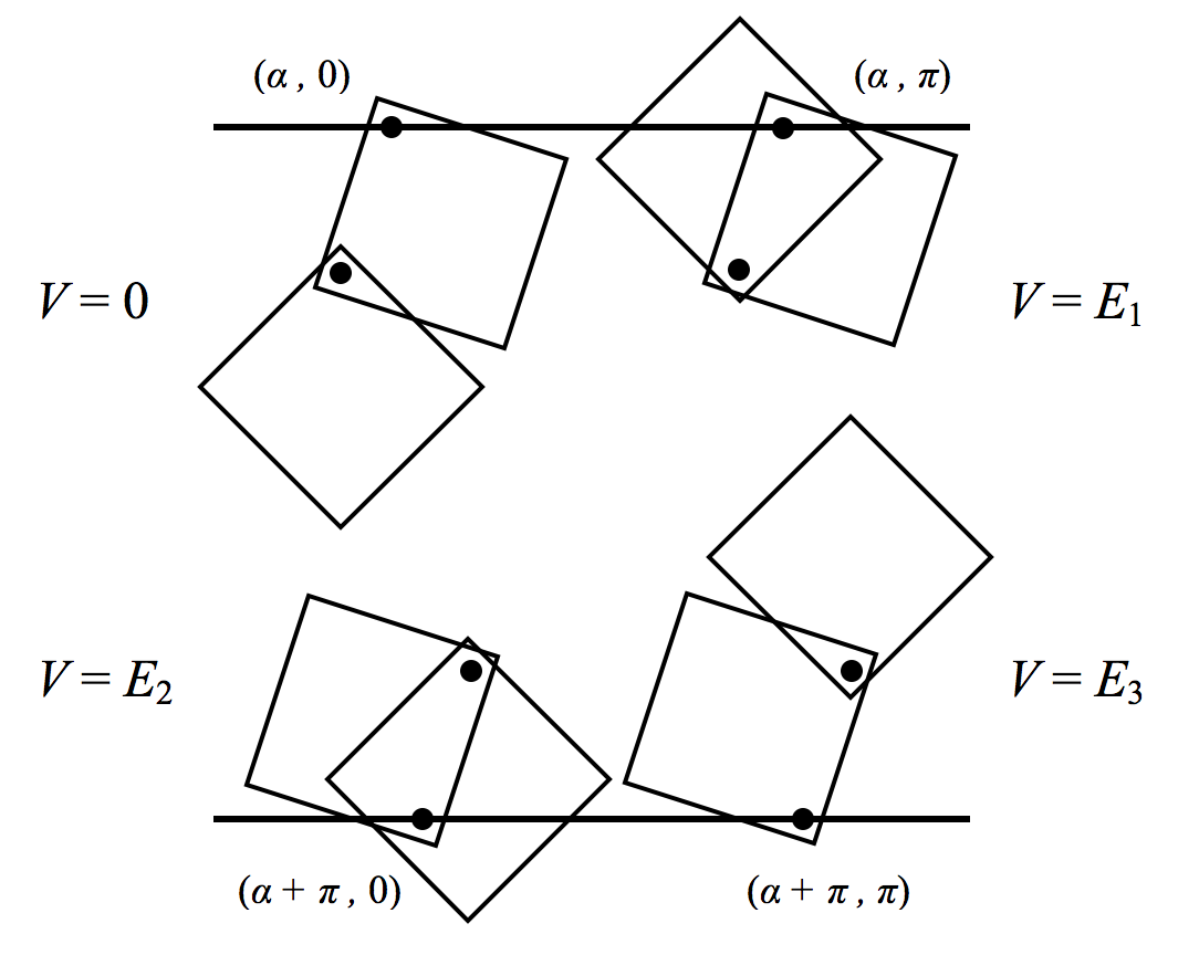
Fig. 3: The equilibrium configurations of the double square pendulum, with the stable equilibrium at upper left. The axles $P$ and $Q$ are indicated by black circles, and the angles $(\theta_{1},\theta_{2})$ and potential energies of the configurations are also shown.

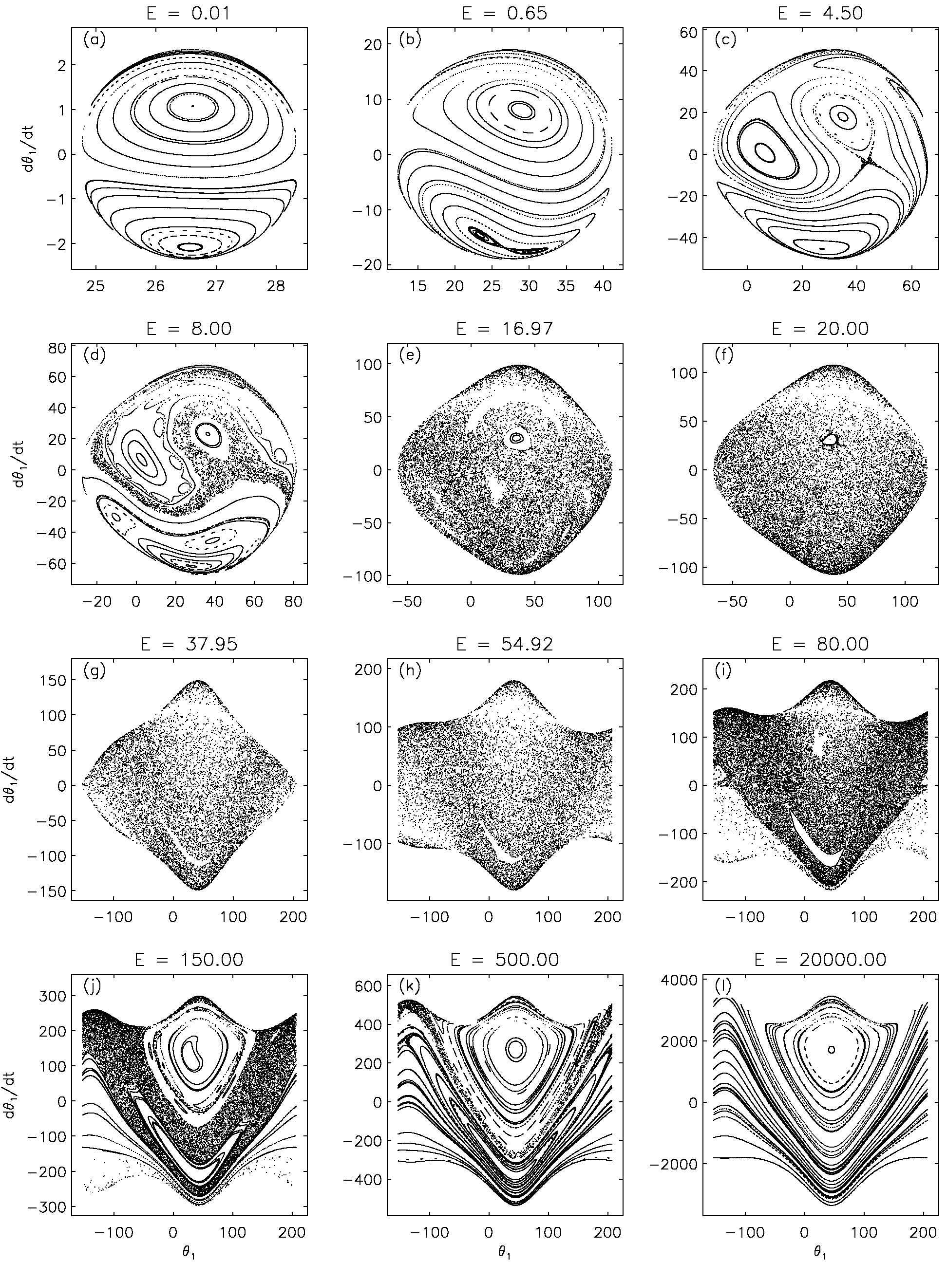
Fig. 4: Poincaré sections of the double square pendulum for increasing values of the dimensionless total energy $E$. The panels show: (a) $E=0.01$; (b) $E=0.65$; (c) $E=4.50$; (d) $E=8$; (e) $E=E_{1}=16.97$; (f) $E=20$; (g) $E=E_{2}=37.95$; (h) $E=E_{3}=54.92$; (i) $E=80$; (j) $E=150$; (k) $E=500$; and (l) $E=20000$.

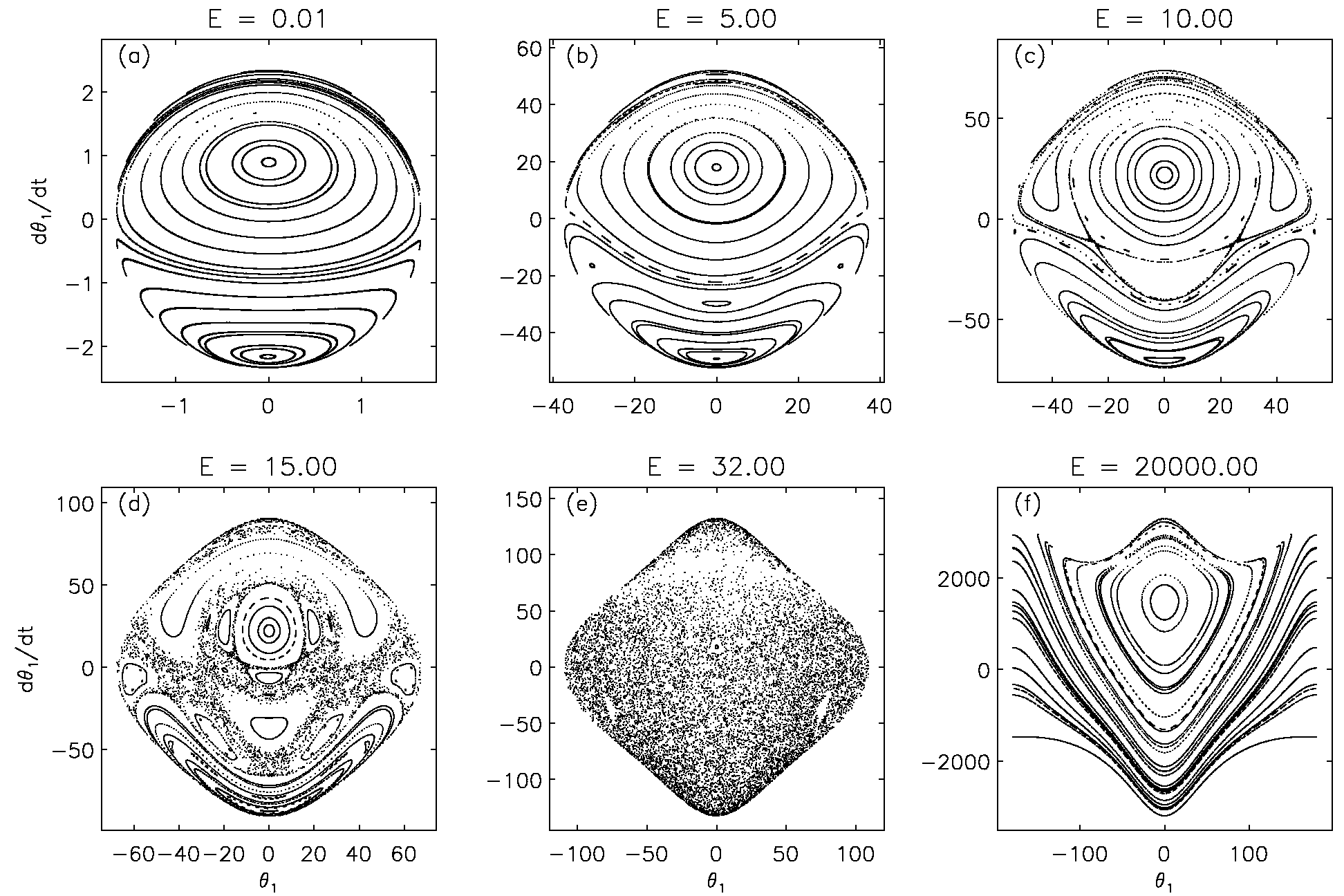
Fig. 5: Poincaré sections of the simple double pendulum for increasing values of $E$. The panels show: (a) $E=0.01$; (b) $E=5$; (c) $E=10$; (d) $E=15$; (e) $E=32$; and (f) $E=20000$.

References

- (1) P. H. Richter and H. -J. Scholz, “Chaos in classical mechanics: The double pendulum,” in Stochastic Phenomena and Chaotic Behavior in Complex Systems, edited by P. Schuster (Springer, Berlin, Heidelberg, 1984), pp. 86–97.
- (2) H. J. Korsch and H. -J. Jodl, Chaos: A Program Collection for the PC (Springer-Verlag, Berlin, 1999), 2nd ed.
- (3) T. Stachowiak and T. Okad, “A numerical analysis of chaos in the double pendulum,” Chaos, Solitons and Fractals 29, 417–422 (2006).
- (4) L. D. Landau and E. M. Lifshitz, Mechanics (Elsevier, Amsterdam, 1976), 3rd ed.
- (5) H. Goldstein, Classical Mechanics (Addison-Wesley, Reading MA, 1980), 2nd ed.
- (6) T. W. B. Kibble and F. H. Berkshire, Classical Mechanics (Imperial College Press, London, 2005), 5th ed.
- (7) R. D. Gregory, Classical Mechanics (Cambridge University Press, Cambridge, 2006).
- (8) P. K. Newton, “Escape from Kolmogorov-Arnold-Moser regions and breakdown of uniform rotation,” Phys. Rev. A 40, 3254–3264 (1989).
- (9) R. B. Levien and S. M. Tan, “Double pendulum: An experiment in chaos,” Am. J. Phys. 61, 1038–1044 (1993).
- (10) T. Shinbrot, C. Grebogi, J. Wisdom, and J. A. Yorke, “Chaos in a double pendulum,” Am. J. Phys. 60, 491–499 (1992).
- (11) Z. Zhou and C. Whiteman, “Motions of double pendulum,” Nonlinear Analysis, Theory, Method and Applications 26 (7), 1177–1191 (1996).
- (12) A. Ohlhoff and P. H. Richter, “Forces in the double pendulum,” Z. Angew. Math. Mech. 80 (8), 517–534 (2000).
- (13) Available at <http://www.chaoticpendulums.com/>.
- (14) H. R. Dullin, “Melkinov’s method applied to the double pendulum,” Z. Phys. B 93, 521–528 (1994).
- (15) Movies showing the double square pendulum in action are available at <www.physics.usyd.edu.au/~wheat/sdpend/>.
- (16) L. N. Hand and J. D. Finch Analytical Mechanics (Cambridge University Press, Cambridge, 1998).
- (17) I. G. Main, Vibrations and Waves in Physics (Cambridge University Press, Cambridge, 1984), 2nd ed.
- (18) W. H. Press, B. P. Flannery, S. A. Teukolsky and W. T. Vetterling, Numerical Recipes in C (Cambridge University Press, New York, 1992), 2nd ed.
- (19) P. G. Drazin, Nonlinear Systems (Cambridge University Press, Cambridge, 1992).
- (20) R. C. Hilborn, Chaos and Nonlinear Dynamics: An Introduction for Scientists and Engineers (Oxford University Press, New York, 2000), 2nd ed.
- (21) Animations of the numerical solution of the equations of motion for different energies corresponding to some of the choices in F ig. 4 are available at <www.physics.usyd.edu.au/~wheat/sdpend/>.
- (22) T. Tél and M. Gruiz, Chaotic Dynamics: An Introduction Based on Classical Mechanics (Cambridge University Press, Cambridge, 2006).
- (23) A movie showing nearly aligned frames for three releases of the pendulum is available at <www.physics.usyd.edu.au/~wheat/sdpend/>.