The Calibration of Strömgren $uvby$-H$\beta$ Photometry for Late-Type Stars – a Model Atmosphere Approach

Abstract

Context. The use of model atmospheres for deriving stellar fundamental parameters, such as $T_{\rm eff}$, $\log g$ and [Fe/H], will increase as we find and explore extreme stellar populations where empirical calibrations are not yet available. Moreover calibrations for upcoming large satellite missions of new spectrophotometric indices, similar to the $uvby-$H$\beta$ system, will be needed.

Aims. We aim to test the power of theoretical calibrations based on a new generation of MARCS models by comparisons with observational photomteric data.

Methods. We calculate synthetic $uvby-$H$\beta$ colour indices from synthetic spectra. A sample of 388 field stars as well as stars in globular clusters is used for a direct comparison of the synthetic indices versus empirical data and for scrutinizing the possibilities of theoretical calibrations for temperature, metallicity and gravity.

Results. We show that the temperature sensitivity of the synthetic $(b-y)$ colour is very close to its empirical counterpart, whereas the temperature scale based upon H$\beta$ shows a slight offset. The theoretical metallicity sensitivity of the $m_{1}$ index (and for G-type stars its combination with $c_{1}$) is somewhat larger than the empirical one, based upon spectroscopic determinations. The gravity sensitivity of the synthetic $c_{1}$ index shows a satisfactory behaviour when compared to obervations of F stars. For stars cooler than the sun a deviation is significant in the $c_{1}$–$(b-y)$ diagram. The theoretical calibrations of $(b-y)$, $(v-y)$ and $c_{1}$ seem to work well for Pop II stars and lead to effective temperatures for globular cluster stars supporting recent claims by Korn et al. (2007) that atomic diffusion occurs in stars near the turnoff point of NGC 6397.

Conclusions. Synthetic colours of stellar atmospheres can indeed be used, in many cases, to derive reliable fundamental stellar parameters. The deviations seen when compared to observational data could be due to incomplete linelists but are possibly also due to effects of assuming plane-parallell or spherical geometry and LTE.

1 Introduction

The $uvby$ photometric intermediate-band system of Strömgren (1963) and the H$\beta$ narrow-band system (Crawford 1958, 1966) were combined early and soon proved to be a most powerful means of determining fundamental parameters of stars. Calibrations of the systems were also developed early by Strömgren, Crawford and collaborators. Generally, semi-empirical methods were used with the calibrations made by means of sets of stars with parameters determined in more fundamental ways. The first metallicity calibration of the $m_{1}$ index for solar-type stars by Strömgren (1964) was thus based on spectroscopical [Fe/H] values of Wallerstein (1962) and the first luminosity calibration of the $c_{1}$ index by Strömgren (see Crawford 1966) used cluster stars in the main-sequence band. This general semiempirical approach continued with calibrations like those of the $m_{1}$ index by Nissen (1970), Gustafsson $\&$ Nissen (1972), Nissen $\&$ Gustafsson (1978) and Nissen (1981) where very-narrow-band spectrophotometry of groups of weak lines was calibrated with synthetic spectra. These stars were then used as calibration stars for $uvby$-H$\beta$ photometry. Other calibrations follow this semiempirical approach e.g. those of Crawford (1975), Ardeberg $\&$ Lindgren (1981) and Olsen (1988) for G and K-type stars, as well as by Schuster & Nissen (1989) for metal-poor stars. In the calibration by Alonso et al. (1996) the effective temperature calibration was based on stellar temperatures from the Infrared Flux Method. The calibrations by Nordström et al. (2004) and Holmberg et al. (2007) additionally utilised Hipparcos parallaxes for the surface gravity calibration.

Another development towards calibration of the systems also started early: the direct calculation of photometric indices by means of model atmospheres. Such theoretical calibrations were attempted for early-type stars with relatively line-free spectra. For late type stars, a statistical correction for the effects of spectral lines was made by Baschek (1960) in his calibration of the Strömgren $m$ index (a predecessor to $m_{1}$). A first systematic and detailed calculation of $uvby-$H$\beta$ indices for a grid of F and G dwarf model atmospheres was published by Bell (1970), using scaled solar model atmospheres. Bell $\&$ Parsons (1974) calculated $uvby$ colours for flux-constant model atmospheres of F and G supergiants, while Gustafsson $\&$ Bell (1979) produced theoretical colours in a number of systems, including the $uvby$ system, for a grid of giant-star model atmospheres. Relya & Kurucz (1978) calculated $uvby$ and $UBV$ colours from early ATLAS models, and discussed their shortcomings for late-type stars. $uvby$ colours for new sets of Kurucz models were published by Lester, Gray $\&$ Kurucz (1986). Castelli $\&$ Kurucz (2006) published H$\beta$ indices. Sometimes, semiempirically corrected fluxes from model atmospheres have also been used for calibrations of Strömgren photometry, see e.g. Lejeune et al. (1999) and Clem et al. (2004).

The need for reliable calibrations of $uvby-$H$\beta$ photometry has increased in the last decade, not the least for estimating parameters of new and more ”exotic” stars, such as very metal-poor and super-metal-rich stars which are not found at great abundance in the solar neigbourhood so that relatively complete sets of calibration stars cannot easily be established. Furthermore, the preparation for the Gaia satellite includes a careful analysis of the power of model atmospheres to provide a detailed astrophysical calibration of the photometric system of the satellite. This analysis needs support by a detailed test of the problems and possibilities to make a detailed theoretical calibration of, e.g., the $uvby-$H$\beta$ photometry.

Subsequently, we shall present the theoretical models and colours (Sect. 2 and 3). Stellar samples for empirical comparisons are discussed in Section 4. Next, the discussion will be focused on the determination of effective temperature, metallicity and surface gravity of the stars, by discussing the calibration of $(b-y)$ and H$\beta$ indices (Sect. 5, effective temperature), of $m_{1}$ (Sect. 6, metallicity) and $c_{1}$ (Sect. 7, gravity) indices, devoting more limited interest to ”secondary” effects such as the metallicity sensitivity of $(b-y)$ and $c_{1}$, or the gravity sensitivity of $m_{1}$. In each section the results will be compared with empirical and semi-empirical data and calibrations. Finally, in the last Section some comments will be made on the success and the problems of the theoretical calibrations, conclusions will be drawn and recommendations given.

2 Model atmospheres and calculated spectra

The theoretical tools used in modelling the stellar colours are model stellar atmospheres and their calculated fluxes. These are based on extensive atomic and molecular data. Here, we shall briefly present the models and data used and refer to more complete descriptions.

2.1 Model atmospheres

The stellar atmosphere code MARCS (Gustafsson et al. 2008, http://marcs.astro.uu.se) was used to construct a grid of 168 theoretical 1D, flux constant, radiative + mixing-length convection, LTE models with fundamental atmospheric parameters as follows: $T_{\rm eff}$ = 4500, 5000, 5500, 6000, 6500 & 7000 K, $\log g$ = 2.0, 3.0, 4.0, 4.5 and [Me/H] = 0.5, 0.0, –0.50, –1.0, –2.0, –3.0, –5.0, [Me/H] denoting the logarithmic over-all metallicity with respect to the sun. Plane parallell (ppl) stratification was assumed for $\log g$ = 4.5, 4.0 & 3.0, whereas spherical (sph) symmetry was assumed for $\log g$ = 2.0. For the spherically symmetric models a mass of 1 M_⊙ was adopted. The local mixing-length recipe was used to describe convective fluxes, for more details see Gustafsson et al. (2008).

Elemental abundances were adopted from Grevesse and Sauval (1998) except for the CNO abundances which were adopted following Asplund et al. (2005).

2.2 Synthetic spectrum calculations

In order to calculate synthetic spectra of sufficiently high resolution the Uppsala BSYN code was used with the MARCS models as input. The spectra were calculated within the wavlength limits of the Strömgren $uvby$ filters with wavelength steps of 0.02 Å. The mictroturbulence parameter, $\xi_{t}$, was set to 1.0 km s^-1 and 1.7 km s^-1, when calculating spectra based on ppl models and sph models, respectively. The effects of changing $\xi_{t}$ are studied in Section 6.

2.3 Line lists

We collected atomic line data from the Vienna Atomic Line Data Base, VALD (version I, Kupka et al. 1999). For hydrogen line data a version of the code HLINOP was used, and has been described by Barklem & Piskunov (2003). This code has been developed based on the original HLINOP by Peterson & Kurucz (see http:// kurucz.harvard.edu/). The hydrogen line profiles are calculated including Stark broadening, self-broadening, fine structure, radiative broadening, and Doppler broadening (both thermal and turbulent). The Stark broadening is calculated using the theory of Griem (1960 and subsequent papers) with corrections based on Vidal et al. (1973). Self-broadening is included following Barklem et al (2000) for H$\alpha$, H$\beta$ and H$\gamma$, while for other lines the resonance broadening theory of Ali & Griem (1966) is used. For molecules, data for C₂ including ¹²C¹³C lines were gathered from Querci, Querci & Kunde (1971) and Querci (1998, private communication with B. Plez), except for the Fox-Herzberg band in the UV for which data was taken from Kurucz (1995). Molecular data for CH with ¹³CH comes from Plez et al. (2008) and Plez (2007, priv. communication). Data for the CN molecule with ¹²C¹⁵N, ¹³C¹⁴N, and ¹³C¹⁵N are also from Plez (priv. communication). CO data with ¹³C¹⁶O was gathered from Kurucz (1995) as well as NH with ¹⁵NH, OH with ¹⁸OH, and MgH with ²⁵MgH and ²⁶MgH. TiO was not taken into account in the calculations since absorption by this molecule is expected to have small effects on the spectra within the effective-temperature range considered.

3 Colour index calculations

3.1 Filter profiles

To determine the theoretical $m_{1}$, $c_{1}$ and $(b-y)$ indices, transmission profiles of the Strömgren $uvby$ filters (Crawford & Barnes (1970) see Fig. 1) were multiplied with the calculated model stellar surface flux within the wavelength range of the filters:

$$mag\,=\,-2.5\,{\rm\log}\left(\frac{\int{F_{\lambda}T_{\lambda}d\lambda}}{\int{T_{\lambda}d\lambda}}\right)+const.$$

where $F_{\lambda}$ and $T_{\lambda}$ are the flux and the relevant transmission profile, respectively. The theoretical magnitudes were converted into colour indices via the definitions: $c_{1}\equiv u-2v+b,\,\,m_{1}\equiv v-2b+y.$

The H$\beta$ index is defined (Crawford 1958) as the ratio of the flux measured through a narrow and a wide profile, respectively, both centered around the H$\beta$ line:

$${\rm H}\beta\,=\,-2.5\left(\log\frac{\int{F_{\lambda}T_{N,\lambda}d\lambda}}{\int{T_{N,\lambda}d\lambda}}-\log\frac{\int{F_{\lambda}T_{W,\lambda}d\lambda}}{\int{T_{W,\lambda}d\lambda}}\right)+const.$$

where $T_{W,\lambda}$ and $T_{N,\lambda}$ are the wide and the narrow filter profiles, respectively. We have found notable differences between synthetic H$\beta$ indices calculated with the Kitt Peak filter set denoted (9, 10) and those calculated with the (212, 214) set, both described by Crawford & Mander (1966, CM66). Here, the Kitt Peak (212, 214) filter system was chosen (Fig. 1 CM66) with a transmission function adopted from Castelli & Kurucz (2006), see Figure 1.

Figure 1: The $uvby-$H$\beta$ transmission functions of the standard systems plotted as a function of wavelength. As a comparison, the flux (per Ångström unit) of a model with $T_{\rm eff}$ = 6000 K, $\log g$ = 4.0 and [Me/H] = 0.0 is plotted on an arbitrary flux scale.

3.2 Transformation to the observational system

The frequent use of filter-profiles different from those that originally have defined the photomteric system needs some extra considerations. For the H$\beta$ index this mainly comes in at the zero-point determination. Since the observed indices are defined on a system with zero-points set by particular standard stars, we must apply corresponding zero-point shifts to our theoretical system. The much observed, and frequently used, star Vega was chosen to estimate these zero-points. Thus, a model atmosphere for Vega was calculated with parameters $T_{\rm eff}$ = 9550 K, $\log g$ = 3.95 and [Me/H] = –0.5 (mean values of selected measurements presented in SIMBAD), and a synthetic spectrum was computed. Theoretical indices for the Vega model were calculated and compared to observed values: $c_{1}$ = 1.088, $m_{1}$ = 0.157 and $(b-y)$ = 0.003 (Hauck and Mermilliod 1998). The resulting differences between the theoretical and observed colours were then added as constants to all calculated Strömgren colours in our model grid.
For the H$\beta$ index, Crawford & Mander (1966) presented several filter systems, of which we choose the (212, 214) filters as mentioned above. Indices calculated by using this filter set, which are referred to as H${}^{\prime\prime}\beta$ below, should be transformed via a set of equations (CM66), in order to agree with previous Crawford–Mander observations on their standard system. The transformation for the (212,214) filters is described by the following two equations (CM66, Table III):

H$\beta=0.374+1.305\,$H${}^{\prime}\beta$,   B stars

H$\beta=0.248+1.368\,$H${}^{\prime}\beta$,   A, F stars,

derived from a set of 45 and 35 bright stars, where H${}^{\prime}\beta$ and H$\beta$ are the observed and tranformed indices, respectively. The later equation for A and F stars was applied on all H$\beta$ indices in our theoretical grid.

The A0 star Vega clearly poses a number of problems for determining the zero-point of the $uvby$ and H$\beta$ indices. It is known to be rapidly rotating, but with its axis close to the line of sight (Gulliver, Hill & Adelman 1994, Hill, Gulliver & Adelman 2004). Vega has also been regarded to show mild $\lambda$ Bootis star characteristics, such as certain non-solar abundance ratios as well as dust emission in the IR (see Gigas 1988, Hill 1995, Ilijic et al. 1998, Adelman & Gullliver 1990, Heiter, Weiss & Paunzen 2002). However, these departures from standard A0 stars, as well as standard model atmospheres, are thought to only lead to minor modifications of its $uvby-$H$\beta$ indices (Paunzen et al. 2002). A more practical problem is that neither of the two CM66 transformation equations from H${}^{\prime}\beta$ to H$\beta$ will give a fully satisfactory fit due to the fact that the index for Vega should be transformed intermediately between the B star and the A, F star sets. Several tests were performed which all pointed in the direction that Vega should be transformed to the standard system via an equation somewhere in between the B and the A, F transformations but with a heavier weight for the latter. By using all listed A0 stars in Table II of CM66, a special transformation between H${}^{\prime}\beta$ and H$\beta$ for A0 dwarf stars was established, as can be seen in Figure 2. The vertical line in the plot represents the observed H$\beta$ value for Vega (Hauck & Mermilliod, 1998). However, the observed H${}^{\prime}\beta$ value of Vega is not known. In order to determine the zero point c in the transformation from calculated (H${}^{\prime\prime}\beta$) to “observed” H${}^{\prime}\beta$ values, H${}^{\prime\prime}\beta$ = H${}^{\prime}\beta$ + c, we have therefore adopted an H${}^{\prime}\beta$ value for Vega derived from the A0 stars line in Figure 2, read off at the observed H$\beta$ for the star. After correction of the model H${}^{\prime\prime}\beta$ value to H${}^{\prime}\beta$ we have then calculated the model H$\beta$ values by using the empirical A,F-transformation relation as mentioned earlier.

Figure 2: H$\beta$ and H${}^{\prime}\beta$ values for A0 stars tabulated in CM66 are plotted individually and represented by a linear regression (thick line), as well as the transformation relations for B and A+F stars, respectively, following CM66 (thin lines).

The transmission functions of the filters used by Olsen (1983, 1984) and Schuster & Nissen (1988) depart from those on which the system was originally based (Crawford 1966). Filter profiles representative for these newer studies are given by Helt et al. (1987) and Bessell (2005). In particular, the more recent $v$ band is narrower, and its effective wavelength shifted by about 25 Å towards the red. To test the effects of this, we have calculated colours with the Helt et al. (1987) profiles as an alternative to the Crawford set, and then applied the transformations as given by Schuster & Nissen (1988) back to the standard system to mimic the procedure of the observers. From this, we find changes of the calculated values, amounting to typically 0.02 magnitudes or less in the $m_{1}$ and $c_{1}$ index values and only 0.002 in $(b-y)$. In particular, the changes in the differential values measuring the sensitivity of $m_{1}$ to metallicity and of $c_{1}$ to gravity are small, in $\delta m_{1}/\delta$[Me/H] typically 0.003 and in $\delta c_{1}/\delta\log g$ typically 0.01. Such effects do not change our conclusions in the present paper.

3.3 Model colours

The model colours, with zero-point added using Vega observations, are supplemented the present paper electronically.

4 Comparison star samples

In order to test the reliability of our calculated colours, we selected a sample of standard stars. These were taken from various sources: one subset with well determined spectroscopic parameters was selected from The Bright Star Catalogue (Hoffleit & Warren 1995), another from the $uvby$ standard stars listed by Crawford & Barnes (1970), a third from the list of metal-poor stars in Schuster & Nissen (1988), a fourth among stars that have been observed by the Hubble-STIS spectrograph and a fifth from the stars listed in the study of Pop II stars by Jonsell et al. (2005). Altogether 388 stars were thus selected. The fundamental parameters were taken from the sources listed, or from other sources given in the SIMBAD catalogue and judged to have high quality. Complementary photometry was also obtained from SIMBAD. Parameter determinations based on $uvby-$H$\beta$ photometry were avoided as far as possible, since we aimed at testing calibrations based on this photometric system relative to parameters based on more fundamental methods. In practice, this usually means effective temperatures based on the infrared-flux method and gravities and metallicities based on high-resolution spectroscopy. The effective temperatures gathered from the Jonsell et al (2005) sample are calculated with the Alonso et al. (1996) calibration. These stars however, constitute less than 5 % of our total sample. In the case of multiple sources, i.e., stellar values listed in more than one of our selected catalogues, a mean value was used. The $uvby$ indices of the standard stars were dereddened by means of the algorithm and computer code of Hakkila (1997). For most of the stars, in particularly the dwarfs, $E$(B-V) was smaller than $\sim$0.01.

Altogether, the standard stars span a volume in the parameter space ranging from 3900 K to 7850 K in $T_{\rm eff}$, 0.20 to 4.80 in $\log g$ (cgs units) and –3.0 dex to 0.45 dex in [Fe/H]. Data for the full standard sample is accessible electronically from A&A as on-line material supplementing the present paper. As seen in Figure 3 our standard sample satisfactorily covers the fundamental parameter space, although one would need some more cool ($T_{\rm eff}<5000$) and hot ($T_{\rm eff}>6300$) dwarf stars ($\log g>4.0$). For this purpose two complementary homogeneous samples were tested; the stellar sample published by Casagrande et al (2006, hereafter C06) and Valenti & Fischer (2005, hereafter VF05). $uvby$ colour indices for both samples were taken from Hauck & Mermilliod (1998). These complimentary stellar samples cover the parameter spaces: $4700\leq T_{\rm eff}\leq 6600$, $3.1\leq\log g\leq 5.1$ and $-1.9\leq\rm[Fe/H]\leq 0.5$ for the VF05 sample and $4406\leq T_{\rm eff}\leq 6556$, $\log g\sim 4.5$ and $-1.87\leq\rm[Fe/H]\leq 0.34$ for the C06 sample. Despite that the lowest $\log g$ values in the VF05 sample are characteristic of giants/sub-giants, a majority (93 %) of the VF05 stars are dwarfs with $\log g\geq 4.0$. In the C06 sample all stars are assumed to be dwarfs with $\log g\sim 4.5$. A majority (85 %) of the stars in the VF05 sample are also metal-rich, [Fe/H] $\geq-0.2$, whereas the C06 sample is evenly distributed in metallicity. Likewise, the effective temperatures of the C06 sample (determined by the authors’s new calibration of the infrared-flux method) are evenly distributed but the VF05 sample is biased towards higher temperatures, $T_{\rm eff}\geq 5500$ (74 %). Among the stars in the standard sample, 18 and 72 are found in the C06 and VF05 samples, respectively. For the stars in the VF05 sample no significant trends of discrepacies for the values given, $T_{\rm eff}$, $\log g$ and [Fe/H], were found. In the C06 sample we find an overall difference in given effective temperatures, growing for higher effective temperatures at low metallicities ($T_{\rm eff\,standard}-T_{\rm eff\,Casagrande}\approx-175$ K at $T_{\rm eff}\sim 6000$ K and $-2.0\leq$ [Fe/H] $\leq-1.0$).

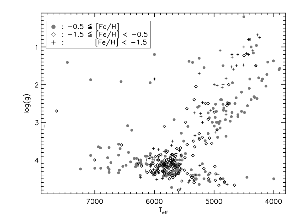
Figure 3: Fundamental parameters, i.e. $T_{\rm eff}$, [Fe/H] and $\log g$, for the standard sample.

5 The effective-temperature calibration

Precise determinations of effective temperatures of stars are critical for a variety of reasons, not only for direct applications such as comparisons of isochrone calculations to observed colour-magnitude diagrams, but also in more indirect applications e.g. determinations of chemical abundances. Photometric indices play a critical role when determining the effective temperatures of stars. For stars located on the main sequence, model atmosphere calibrations of these indices may be particularly important since determinations of diameters are generally few and poor.
The Strömgren $(b-y)$ index provides a sensitive temperature measure for F, G and K stars. The H$\beta$ index is another frequently used criterion for deriving temperatures. We study both indices here.

In Figure 4 (left) we explore the temperature sensitivity of the theoretical $(b-y)$ index for different metallicities. As a comparison we also plot $(b-y)$ for a set of Kurucz models (Lester, Gray & Kurucz, 1986). We note that the indices, calculated with the different model sets, more or less show the same behaviour although the models of Lester et al. are systematically bluer at given $T_{\rm eff}$. In comparison with observed values for stars our synthetic indices show a satisfactory temperature sensitivity over the full temperature range (4500–7000 K), see Figure 5.
In Figure 4 (right) the H$\beta$ index is plotted versus effective temperature, together with the theoretical data of Castelli & Kurucz (2006). For the warmer part of the temperature range we find no differences in sensitivity, whereas for the cooler temperatures (5500 K) we note that MARCS indices have a steeper gradient, thus lower H$\beta$ values than those of Castelli & Kurucz. Our steeper gradient tends to agree with observed stellar colours, Figure 6, which is probably due to improvements of the broadening theory of H$\beta$.

Figure 4: The $(b-y)$ colour index (left) and H$\beta$ index (right) versus effective temperature for MARCS and Kurucz (Lester, Gray & Kurucz (1986), LGK, Castelli & Kurucz, 2006, CK) model atmospheres with different [Me/H] and $\log g$ (indicated to the left and right of each curve). Corresponding theoretical MARCS $(b-y)$ and H$\beta$ curves for [Me/H] = 0.5, –0.5, and –3.0 can be seen in Figure 5 and Figure 6, respectivley.

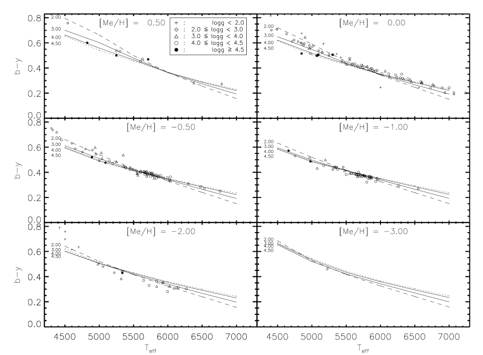
Figure 5: Theoretical $(b-y)$ values versus effective temperature for models with different [Me/H] and $\log g$ plotted together with values for the standard stars (with [Fe/H] within $\pm$0.1 dex of the given [Me/H]). To guide the eye the theoretical $\log g$ curves for 2.0 and 4.5 are plotted as a dashed and a dotted line, respectively.

Figure 6: Theoretical H$\beta$ values versus effective temperature for models with different [Me/H] and $\log g$ plotted together with values for the standard stars (with [Fe/H] within $\pm$0.1 dex of the given [Me/H]). To guide the eye the theoretical $\log g$ curves for 2.0 and 4.5 are plotted as a dashed and a dotted line, respectively.

5.1 $T_{\rm eff}(b-y)$

Several attempts (Alonso et al. 1996, Nordström et al. 2004, Ramírez & Meléndez 2005, Holmberg et al. 2007) have been made to derive empirical calibrations for $uvby-$H$\beta$ colours, where the fundamental parameters are expressed as explicit formulae in the photometric indices. We will here derive such calibration equations by using theoretical colours. We make use of the formal expressions of Alonso et al. (1996, 1999, hereafter A96 resp. A99) based on $(b-y)$ (their eq. 9 and 14 & 15, respectively) but derive new coefficients via an iterative least squares method and by using the model colours.
The result for dwarfs ($\log g\geq 4.0$) are given numerically in Appendix A.1 and can be seen in Figure 7 where we also merge our standard sample with the C06 sample and plot temperatures for the individual stars derived from our theoretical calibration equation. The standard deviations for our calculated temperatures with respect to literature values can be found in Table 1 A linear regression for the calculated temperatures of the two merged samples is also shown in Figure 7 and yields a dispersion $\sigma$ = 117 K. We note that our theoretical calibration gives higher temperatures, as compared with literature values, by $\sim$100 K for the cooler stars ($T_{\rm eff}$$\,<\,$5000 K) and tends to lead to lower temperatures ($\sim$100–150 K) than the values found in the literature for hotter stars ($T_{\rm eff}$$\,>\,$6500 K). Our calibration suggests lower temperatures than the values listed in VF05 by 100-200 K for stars within the range of 5200-6300 K. Below that our theoretical calibration gives systematically $\sim$100 K higher temperatures for the VF05 stars, in accordance with the tendencies found also for the other comparison samples. The standard deviation of the calculated temperatures for the VF05 sample can be seen in Table 1.

It is also interesting to compare our results to previous empirical calibrations. The standard deviations of the calculated temperatures using four different empirical calibrations applied on our three comparison samples, are listed in Table 1. In order to illustrate the empirical trends the resultant linear regressions for the merged standard and C06 samples are shown in Figure 7 (note the shifted scale by 1000 K).

Table 1: Standard deviations for $T_{\rm eff}$ and [Fe/H] derived using models as compared with literature values of the different comparison samples.

		$T_{\rm eff}$		[Fe/H]
	Dwarfs		Giants	G-stars	F-stars
Theoretical	$(b-y)$	H$\beta$	$(b-y)$
Standard	133	151	144	0.263	0.254
C06	101	—	—	0.321	0.190
VF05	185	—	—	0.392	0.399
All	172	—	—	0.368	0.355
A06,99 + S&N89	A06		A99	S&N89
Standard	110	156	116	0.183	0.182
C06	118	—	—	0.158	0.128
VF05	135	—	—	0.128	0.146
All	130	—	—	0.141	0.157
HNA07
Standard	101	—	—	0.208	0.164
C06	92	—	—	0.159	0.132
VF05	101	—	—	0.123	0.130
All	100	—	—	0.144	0.140
RM05
Standard	155	—	105	0.268	0.176
C06	110	—	—	0.176	0.139
VF05	128	—	—	0.116	0.081
All	134	—	—	0.161	0.122

The calibration results for giants ($1.5\leq\log g\leq 3.5$) is presented in Appendix A.2 and shown in Figure 8. The standard deviations with respect to effective temperatures of the standard stars are shown in Table 1 together with the standard deviations for the same sample when using the A99 empirical calibration.

5.2 $T_{\rm eff}$(H$\beta$)

A theoretical temperature calibration for dwarfs was also derived for the H$\beta$ index, with a formal expression adopted from A96, Eq. 10, see Appendix A.1. The result can be seen in Figure 9. Standard deviations with respect to the literature values of the standard sample are listed in Table 1, values somewhat higher than the calibration based on $(b-y)$. Here we are, however, using different stars in the $T_{\rm eff}$$(b-y)$ and $T_{\rm eff}$(H$\beta$) equations (fit limits defined in A96). To make a fair comparison between the two calibrations we have restricted our sets of stars to be identical for both calibrations. Such a comparison is made in Sec. 5.3. A linear regression for the calculated effective temperatures is also shown in Figure 9. The dispersion around this fit is $\sigma$ = 143 K. We see that our theoretical calibration suggests somewhat higher effective temperatures, of roughly 100 K, in the cooler part of the temperature range (T_eff $\sim$ 5000 K), and that it possibly implies lower effective temperatures of the order of $\sim$ 100 K for the warmest stars ($T_{\rm eff}$ $>$ 6500 K). Some of these tendencies may possibly be traced also in the $(b-y)-T_{\rm eff}$ calibration (c.f. Fig. 7). As an alternative, the effective temperatures for the standard sample are calculated with the empirical calibration equation by A06. The standard deviations with respect to literature values are presented in Table 1, and a linear regression to the calculated effective temperatures is also plotted in Figure 9.

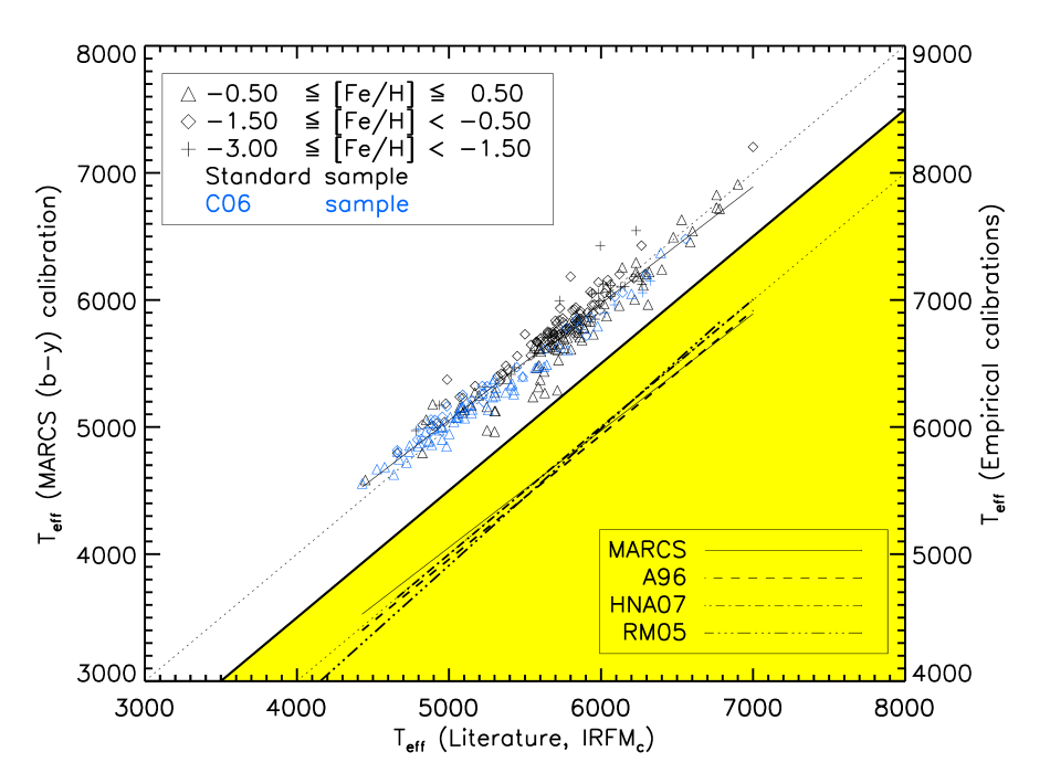
Figure 7: Comparison of calibrations of $(b-y)$ for dwarf stars with individual values for the standard stars and C06 plotted. The solid line represents a fit of the effective temperatures adopted for the stars relative to the corresponding values obtained from the theoretical calibration. Below that (shaded area and right y-axis) corresponding linear regressions of the adopted effective temperatures relative to empirical calibrations (Alonso et al. 1996, Holmberg et al. 2007 and Ramírez & Meléndez 2005) are shown. The dotted line is a one-to-one line.

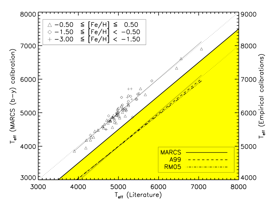
Figure 8: Comparison of calibrations of $(b-y)$ for giant stars with individual values for the standard stars plotted. The solid line represents a fit of the effective temperatures adopted for the standard stars relative to the corresponding values obtained from the theoretical calibration. Below that (shaded area and right y-axis) corresponding linear regressions of the adopted effective temperatures relative to empirical calibrations (Alonso et al. 1999 and Ramírez & Meléndez 2005) are shown. The dotted line is a one-to-one line.

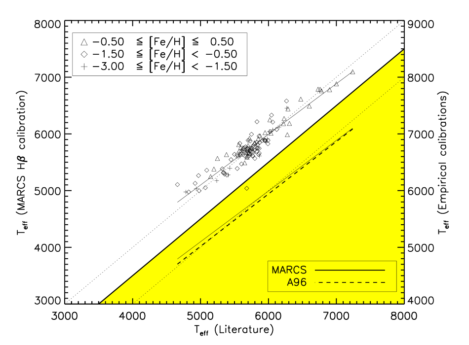
Figure 9: Comparison of calibrations of $T_{\rm eff}({\rm H}\beta)$ for dwarf stars with individual values for the standard stars plotted. The solid line represents a fit of the effective temperatures adopted for the standard stars relative to the corresponding values obtained from the theoretical calibration. Below that (shaded area and right y-axis) a corresponding linear regression of the adopted effective temperautres relative to an empirical calibration (Alonso et al. 1996) is shown. Note that the star located in the shaded area belongs to the theoretical calibration and should therefore be read off at the left y-axis. The dotted line is a one-to-one line.

5.3 $T_{\rm eff}$($b-y$) vs $T_{\rm eff}$(H$\beta$)

Now we compare the derived temperatures based on $(b-y)$ and H$\beta$, respectively. 119 stars matching the restrictions in the parameter space for both calibrations were selected out of our standard sample. The effective temperatures based on $(b-y)$ and H$\beta$ and the result are displayed in Figure 10. The test reveals that there is some disagreement between the two theoretical calibrations. The H$\beta$ based equation suggests higher temperatures for the cooler stars ($T_{\rm eff}$ $\lesssim$ 5000 K) and lower temperatures for the warmer stars ($T_{\rm eff}$ $<$ 6900 K) of some 200 K. The empirical equation of Alonso et al. (1996) shows more or less the same spread for the standard sample but no significant departures from the 1-1 line, which is also to be expected. The failure for the theoretical calibration for the coolest stars is not very remarkable, since the metal lines for those stars are strong and dominate the H$\beta$ line, and other parameters affect the index such as gravity. The departure in the hotter end is only dependent on a few standard stars.
It is worth noting that the difference between the $(b-y)$ and H$\beta$ calibrations responds in opposite directions to different gravities. I.e., the temperature sensitivity $\delta(index)/\delta(T_{\rm eff})$ decreases with increasing gravity for $(b-y)$ while it increases for $T_{\rm eff}\leq 5000\,K$ for H$\beta$ (see Fig. 4). As is seen, these differences are also metallicity dependent, and tend to vanish for small metallicities. However, for stars with known reddening and assuming e.g. the metallicity to be known and relatively large, this may make it possible to obtain a temperature and rough gravity classification from $(b-y)$ and H$\beta$, only.

Figure 10: The effective temperatures calculated by the equations based on H$\beta$ and $(b-y)$. Solid line theoretical fit, dashed line empirical fit (Alonso et al. 1996). The dotted line is the one-to-one relation.

6 The metallicity calibration

The basic aim of $m_{1}\equiv(v-b)-(b-y)$ was to measure the total intensity of the metal lines in the $v$ band. As was early appreciated by Strömgren, for late F and G stars of Pop I these lines are, however, to a large extent located on the flat part of the Curve of Growth and are thus not very sensitive to metallicity, but rather to microturbulence. Moreover, for the hotter stars, the H$\delta$ line is strongly affecting the band, and for stars later than G5, CN lines of the (0,1) band in the Violet System are also significant. Thus, the effects of the value of the mircroturbulence parameter, as well as of the individual CNO abundances, e.g. due to dredge-up of CNO processed material from the interior, must be taken into consideration. Certainly, $m_{1}$ also varies with effective temperature and, to a less degree, with surface gravity.

The variation of the calculated $m_{1}$ with $(b-y)$ and metallicity for the model atmospheres is shown in Figure 11 and compared with calculated indices by Lester et al. (1986). As is seen, the index offers a good discrimination in metallicity except for stars of Extreme Population II for which it only works for the cooler end of the temperature interval. A characteristic measure of the sensitivity of the index to overall metallicity is $(\delta(m_{1})/\delta$[Me/H]$)_{(b-y)}$, where the subscript denotes that the sensitivity is measured at a constant $(b-y)$. This quantity, as measured for models with –3.0 $\leq$ [Me/H] $\leq 0.5$ and $\log g$ $\approx$ 4.5 & 4.0, is given in Table  2.

We may compare the sensitivity of the $m_{1}$ index with the empirical results. However, recent calibrations of the Strömgen photometry, e.g. by Holmberg et al. (2007), contain complex non-linear expressions in which all the indices are involved – in principle a reasonable approach since e.g. also the $c_{1}$ index carries information on the metallicity. Since this metallicity dependence is, however, far from independent of that carried by the $m_{1}$ index the terms in the calibration expressions involving $c_{1}$ may well mask some of the dependence of $m_{1}$ on metallicity. So, as we wish to understand the way $m_{1}$ changes with metallicity, we have instead turned back to the earlier empirical calibrations like that of Nissen (1988), where the metallicity dependence of $m_{1}$ was still treated separately.

Thus, Nissen (1988) finds

$$\rm[Fe/H]=-(10.5+50(H\beta-2.626))\cdot\delta m_{0}+0.12$$ (1)

where $\delta m_{0}$ is calculated as $m_{stand}-m_{1}$ relative to the Hyades standard sequence at constant H$\beta$ and corrected for interstellar extinction. From Figure 11 or Table 2 we may estimate $\delta m_{1}/\delta$[Me/H] at constant $(b-y)$. We can easily calculate the corresponding empirical quantity from the coefficient in Eq. (1) (correcting for the derivative at constant H$\beta$ to constant $(b-y)$ by adding 0.03 which is easily found with sufficient accuracy from the model colours) and then find empirical sensitivities $\delta m_{1}/\delta$[Fe/H] of 0.093 (7000 K) and 0.15 (5750 K), with relevant effective temperatures within parentheses. These values for the sensitivities are valid for [Fe/H]$\approx 0.0$. The corresponding theoretical sensitivities $\delta m_{1}/\delta$[Me/H] for dwarf stars are typically 0.10 and 0.14, respectively. The agreement between the empirical and theoretical results is quite satisfactory. It seems possible that a basic reason why the theoretical calibration, in spite of this agreement, does not succeed very well for the more metal-poor stars (see below) may rather be due to the modelling of the fluxes of those stars than due to failures in calculating the change of flux with metallicity for solar-type stars. It may also be associated with the measured $v$ band being different to that computed, as a single transformation equation is unlikely to correct solar metallicity stars and metal-poor stars by the same amount.

In order to further explore the properties of the calculated $m_{1}$ indices we have plotted individual stars with fairly well-determined fundamental parameters, chosen from our standard sample in the $m_{1}-(b-y)$ diagram. As is seen in Figure 12, these stars match the calculated indices relatively well, although there seems to be a tendency of the sensitivity of the $m_{1}$ index to metallicity to be exaggerated by the model fluxes for the hotter stars. Also, it is clear from Figure 12 that the metal-rich stars lie somewhat low, possibly suggesting that the zero-point of the $m_{1}$ index as determined from Vega may be somewhat in error.

Figure 11: The $m_{1}$ index versus $(b-y)$ for MARCS and Lester, Gray & Kurucz (1986, LGK) model atmospheres. Arrows show the effect of increasing the N abundances by a factor of 3.

Figure 12: The m₁ index versus $(b-y)$ for MARCS models plotted together with standard stars of different gravities in different panels ($\log g$ for the stars within $\pm$0.1 dex of the given $\log g$). The metallicities of the stars are indicated by different symbols.

Table 2: The metallicity sensitivity, $\delta(m_{1})/\delta$[Me/H]$)_{(b-y)}$, for models with $\log g$ = 4.5 & 4.0.

$(b-y)$/[Me/H]	0.5$-$($-$0.5)	$-$1$-$($-$2)	$-$2$-$($-$3)
$\log g$ = 4.5
0.25	0.124	0.031	0.008
0.30	0.145	0.042	0.013
0.35	0.149	0.056	0.028
0.40	0.139	0.098	0.026
0.45	0.136	0.135	0.032
0.50	0.176	0.146	0.048
0.55	0.233	0.127	0.070
$\log g$ = 4.0
0.25	0.125	0.030	0.010
0.30	0.143	0.041	0.014
0.35	0.148	0.059	0.020
0.40	0.137	0.081	0.031
0.45	0.125	0.097	0.052
0.50	0.145	0.100	0.076
0.55	0.198	0.093	0.089

When studying the calculated indices of Lester, Gray & Kurucz (1986) in Figure 11 we find that they reproduce the observed sensitivity of the $m_{1}$ index more successfully than ours. However, these authors have transformed their calculated colours to match a set of standard stars and have thus scaled the amplitude of the $m_{1}$ index by a correction factor to fit the observations. This is the probable reason for the closer agreement of those calculations with observations. We note that our line list is more complete, and that our treatment of the hydrogen line broadening (affecting H$\delta$ and thus the $v$ band) is more accurate.

What is then the reason for our discrepancy for early F stars? We have compared the MARCS model fluxes with observed solar and stellar fluxes from ground-based and space observations (Edvardsson 2008, Edvardsson et al. 2008) and traced probably significant discrepancies in the region 4000  – 5000  , with empirical fluxes of the Sun and solar-type stars being somewhat smaller than model fluxes in the $b$ band, while the blue-violet fluxes from HST/STIS of the more metal-poor stars are clearly in excess of the model fluxes in the violet-blue spectral region. These departures in both the $b$ and $v$ band may conspire to cause the discrepancy in calculated metallicity sensitivity. As discussed by Edvardsson et al. (2008), 3D model simulations suggest that these effects may be due to thermal inhomogeneities in the stellar atmospheres. Other systematic errors in the models, e.g. due to errors in opacities, line data and effects of departures from LTE are probably less significant.

As a further test of our $m_{1}$ indices we will now be guided by the separate metallicity calibrations for F and G stars, respectively, by Schuster & Nissen (1989, eq. 2 & 3, hereafter S&N89). The derived F-star equation is based on the $m_{1}$ and $(b-y)$ index and for the G-star equation the $c_{1}$ index is also included. We derive a calibration expression based upon the form of these equations and using our theoretical colour grid. The results, when applying this to the standard stars and the C06 sample, can be seen in Figures 13 and 14. For F-stars we find standard deviations of derived [Me/H] values compared with literature values for the standard-star sample as given in Table 1. We note, that for the standard sample, our theoretical calibration tends to suggest lower metallicities than the adopted values for a majority of the stars in the sample and increasing differences with increasing metallicity so that the differences amount to typically 0.3 dex at [Me/H] = 0.0. The overall trend might indicate a zero-point problem; a shift of all stars by 0.130 dex gives a lower spread of the calculated metallicities compared to adapted values, $\sigma_{+0.130}$ = 0.217. This is however still not satisfactory in comparison with the empirical equations which generally show smaller spread and imply higher metallicities (see Table 1 and Figure 13). A linear regression for the F-star calibration values to the adopted values for the standard stars and the C06 sample is plotted in Figure 13. The standard deviation for this line fit is $\sigma$ = 0.172 dex. When applying our calibration to the C06 sample we see the same indications as for the standard sample, except for the lower metallicities, where the theoretical calibration suggest somewhat lower metallicities ($\sim$0.05 dex) than derived in C06. However, the 13 F-stars in this sample are too few to allow any definite conclusions. When making use of the 266 F-stars in the VF sample and remembering that this sample is highly biased towards metal-rich dwarf stars ([Fe/H]$>-0.2$ & $\log g>4.0$) we see the same trend as for the standard sample, i.e. our calibration suggests lower metallicities than those given by VF05 (see also Table 1).

For the G-stars we find similar standard deviations for our standard sample with respect to literature values, see Table 1. There is an overall tendency that our theoretical calibration implies lower metallicities than listed in the literature for the metal-rich standard stars. The increasing deviation with increasing metallicity is of the same order as for the F-star calibration, i.e $\approx$ 0.3 dex at [Me/H] = 0.0. By adding 0.190 dex to all stars we would obtain a lower spread, $\sigma_{+0.190}$ = 0.181, which is of the same order as the deviation shown by empirical equations (see Table 1). A linear regression to the calculated metallicities for the standard sample and C06 is plotted as a solid line in the figure ($\sigma$ = 0.200). When using the 69 G-stars in the C06 sample, the result for the standard sample is confirmed, the theoretical calibration suggests lower metallicities for the higher metallicity range ([Fe/H] $>-0.5$) than listed in literature. Applying the calibrations to the 694 G-stars in the VF05 sample, we obtain similar results as for the C06 sample.

For comparison the metallicities of our three comparison samples are calculated with 3 different empirical calibrations. The resulting standard deviations with respect to literature values can be seen in Table 1 and linear regressions when applied to our standard sample can be seen in Figure 13 & 14 for F-stars and G-stars, respectively.

We note in passing that Clem et al. (2004) also found discrepancies between their calculated $m_{1}$ indices and observations. For their coolest models they had to apply upward corrections to their calculated $m_{1}$ indices of 0.1–0.3 mag. Our $m_{1}$ indices depart considerably less from observations but some upward corrections would be needed to fit the coolest stars in Figure 12.

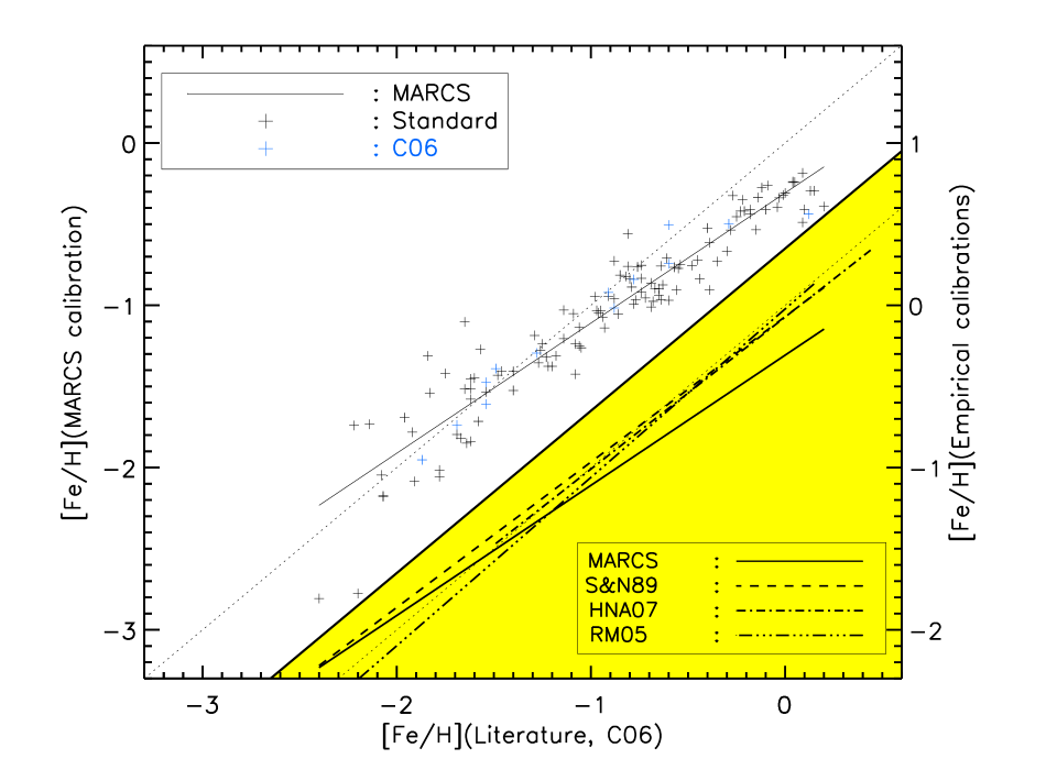
Figure 13: The [Me/H] calibration for F stars from the standard sample and Casagrande et al. (2006, C06). The solid line represents a linear regression of the effective temperatures adopted for the stars relative to the corresponding values obtained from the theoretical calibration. Below that (shaded area and right y-axis) corresponding linear regressions of the adopted effective temperautres relative to empirical calibrations (Schuster & Nissen 1989, Holmberg et al. 2007 and Ramírez & Meléndez 2005) are shown. The dotted line is a one-to-one line.

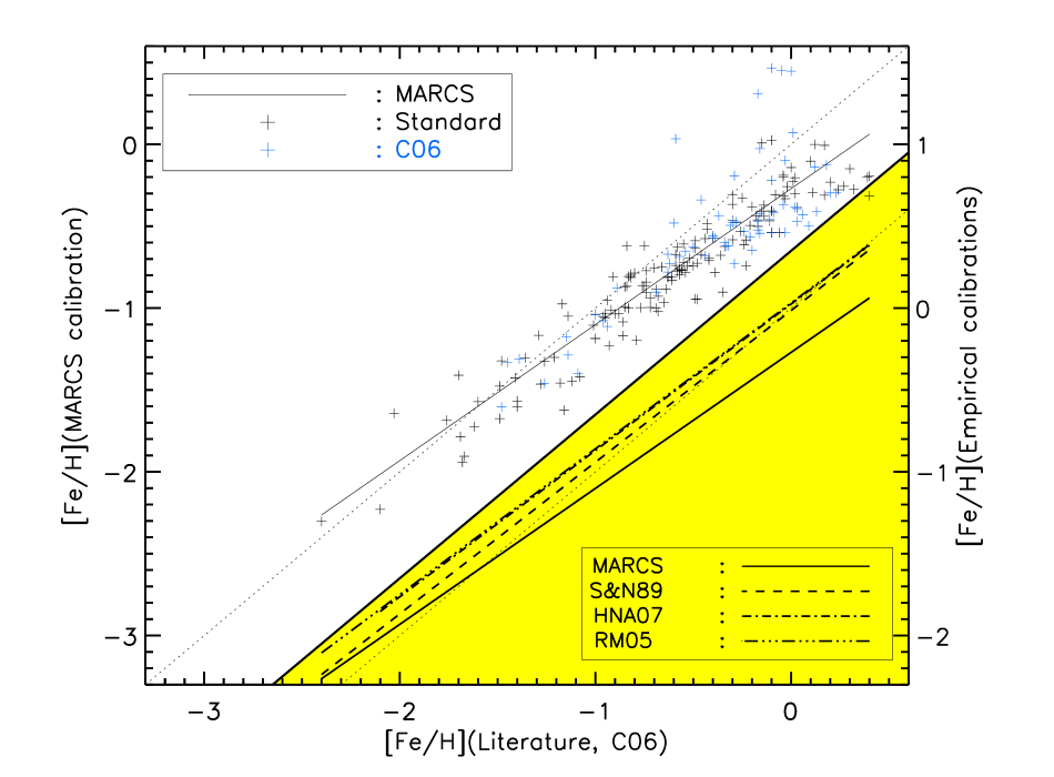
Figure 14: The [Me/H] calibration for G stars. For plot description see Figure 13. Note that empirical calibrations of HNA07 and RM05 overlap and could therefore be difficult to distinguish.

The strong effects of microturbulence on the strengths of the dominating lines in the $v$ band makes it important to investigate whether this could be the reason for the mis-match of the $m_{1}$ index in the theoretical calibration. In Table 3 we examine the effects of changing the microturbulence parameter $\xi_{t}$. The changes have been chosen to be larger for the lower-gravity models to take the larger parameter values usually obtained by spectroscopy for giants into account. We see that the effect of increasing the microturbulence is generally larger for lower $\log g$ and lower temperatures, as expected. When comparing to Figure 12 we see that this effect would indeed improve the situation by shifting the theoretical curves and steepening the curves in the low $T_{\rm eff}$ end. Yet, the effects are considerably smaller than those needed to eliminate the mis-match.

Table 3: The change in the $uvby$ indices when the microturbulence parameter is increased

$\log g$ = 4.0		$\Delta(\xi_{t}\,=\,1.0$	$\rightarrow$	$\xi_{t}\,=\,1.5)$
$T_{\rm eff}$	[Me/H]	$\Delta c_{1}$	$\Delta m_{1}$	$\Delta(b-y)$
4500	0.00	0.0	0.04	0.011
5500	0.00	0.003	0.008	0.005
7000	0.00	0.004	0.005	0.001
4500	$-$1.00	0.006	0.005	0.004
5500	$-$1.00	0.006	0.005	0.002
7000	$-$1.00	0.004	0.002	0.00
$\log g$ = 3.0		$\Delta(\xi_{t}\,=\,1.0$	$\rightarrow$	$\xi_{t}\,=\,2.0)$
$T_{\rm eff}$	[Me/H]	$\Delta c_{1}$	$\Delta m_{1}$	$\Delta(b-y)$
4500	0.00	$-$0.016	0.023	0.032
5500	0.00	0.004	0.025	0.014
7000	0.00	0.001	0.014	0.002
4500	$-$1.00	0.015	0.018	0.012
5500	$-$1.00	0.017	0.013	0.003
7000	$-$1.00	0.006	0.005	0.0

Another circumstance which might have some significance as an explanation for the problems with the $m_{1}$ sensitivity is the effect of lines from the (0,1) band of the CN violet system in the $v$ band. In particular for the cooler giant stars, which may be affected by the first dredge-up of CNO-processed material, the CN lines may become stronger due to this; even if the carbon abundances are reduced by CNO processing, the enhanced N abundance (to which C is converted) makes the CN lines stronger. Also the ¹³CN lines should be significantly enhanced due to the production of ¹³C and N by CNO processing. We have explored these effects by systematically increasing the N abundances by a factor of 3, keeping the C abundance constant. This should lead to an overestimate of the effect, except for possibly stars high-up on the giant branch. As indicated in Figure 11 this only leads to some effects for the more metal-rich giant stars and is not the explanation for the mis-match discussed here.

7 Surface-gravity calibration

The $c_{1}\equiv(u-v)-(v-y)$ index is designed to measure the Balmer discontinuity which is a temperature indicator for B- and A-type stars and a surface-gravity indicator for the late-type stars. Figure 15 shows its behaviour with changing parameters of the models. Obviously, it works nicely as a gravity criterion, with some dependence on metallicity for the most metal-rich stars, which has been a disputed issue in earlier calibration work. We note that for dwarfs cooler than the Sun it seems not very useful as a gravity measure, while for bright giants, and not the least metal-poor ones, it should work down to effective temperatures around 5000 K. In Figure 15 we have also plotted the indices calculated by Lester, Gray & Kurucz (1986). In view of the differences in line data and hydrogen-line theory we find the agreement satisfactory.

Analogously with our treatment of the metallicity dependence of the $m_{1}$ index, we have measured the quantity $\delta c_{1}/\delta\log g$ at constant $(b-y)$ as a measure of the gravity sensitivity of $c_{1}$. Again we have to turn back to earlier calibrations to find corresponding direct empirical measures. Thus, Schuster & Nissen (1989) have elaborated the methodology of Crawford (1975, 1979) and write

$$M_{V}=M_{V,ZAMS}-f\cdot\delta c_{0}$$

$$f\equiv 9.0+38.5\cdot((b-y)_{0}-0.22),$$ (2)

where $0.22\leq(b-y)_{0}\leq 0.47$, $(b-y)_{0}$ being the dereddened $(b-y)$, and $\delta c_{0}$ is the difference of a dereddened $c_{1}$ index and a standard sequence with $M_{V,ZAMS}$ at a given H$\beta$. From this one may estimate the empirical sensitivity $\delta c_{1}/\delta\log g$ to be approximately proportional to $2.5/f$. We thus obtain the following empirical values of ($\delta c_{1}/\delta\log g;\,(b-y)$) for [Fe/H] = 0: (0.21;0.30), (0.16;0.40) and (0.15;0.47). From Figure 15 and Table 4 we measure the corresponding theoretical $\delta c_{1}/\delta\log g$ values to be 0.19, 0.08 and 0.02, respectively. Thus, we find that the empirical gravity sensitivity of the $c_{1}$ index is well reproduced by the hotter models while it becomes underestimated for the cooler ones. We have also compared the calculated $c_{1}$ indices with the observed ones for our samples of standard stars and find a good agreement for the hotter stars (cf. Fig. 16) while for the cooler stars there is a severe mismatch. This is in itself not very remarkable – the total line blocking in the ultraviolet spectra of the cooler stars is considerably greater than $70\%$, and it is to be expected that this will not be very accurately described by the model spectra. The fluxes in the $u$ and $v$ bands are highly sensitive to other parameters, such as microturbulence, and in particular CN abundance for the cooler giants, and these are known to vary systematically with gravity. In fact, as is indicated in Figure 15, the CN line strengthening which is expected for the red giants improves the fit to observed $c_{1}$ indices for the red giant models considerably.

Clem et al. (2004) applied semiempirical corrections also to their calculated $(u-v)$ and $(v-b)$ colours in order to fit observations. The resulting effect on their $c_{1}$ indices is typically less than 0.1 mag while we would need a downward correction of our $c_{1}$ indices of about 0.2 mag for the coolest models to fit (cf. Fig. 16) the metal poor stars and even more for the metal-rich ones.

Figure 15: The $c_{1}$ index versus $(b-y)$ for MARCS and Lester, Gray & Kurucz (1986, LGK) model atmospheres with different $\log g$ values indicated at corresponding curves in the figure and different [Me/H] plotted in different panels. Arrows show the effect of increasing the N abundances by a factor of 3.

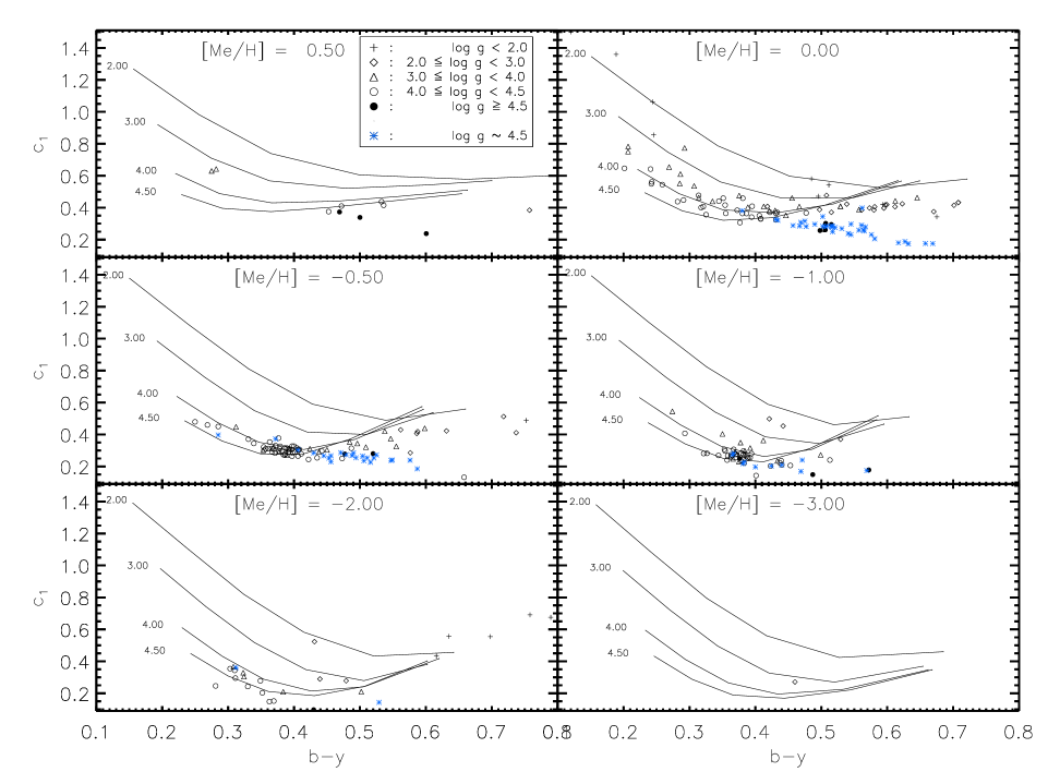
Figure 16: The $c_{1}$ index versus $(b-y)$ for MARCS models with different [Me/H] and $\log g$ plotted together with values for standard stars and Casagrande et al. (2006, C06) stars (marked as asterisks). The [Fe/H] intervals for the standard and C06 stars are [Fe/H] $\pm$0.1 dex and [Fe/H] $\pm$0.2 dex, respectively.

Table 4: The sensitivity to surface gravity, ($\delta c_{1}/\delta\log g)_{(b-y)}$, for models with [Me/H] = $0.5$ and $0.0$

$(b-y)/\log g$	2.0–3.0	3.0–4.0	4.0–4.5
$\rm[Me/H]$ = 0.5
0.25	0.231	0.216	0.207
0.30	0.213	0.187	0.165
0.35	0.183	0.148	0.122
0.40	0.148	0.112	0.091
0.45	0.114	0.086	0.074
0.50	0.083	0.071	0.060
0.55	0.056	0.062	0.049
$\rm[Me/H]$ = 0.0
0.25	0.247	0.230	0.223
0.30	0.236	0.205	0.185
0.35	0.215	0.169	0.131
0.40	0.182	0.126	0.082
0.45	0.144	0.081	0.035
0.50	0.106	0.040	–0.006
0.55	0.065	0.002	–0.026

In a recent article, Twarog et al. (2007) discuss the metallicity dependence of the $c_{1}$ index for disk stars ([Fe/H] $\geq$ –1.00) and conclude that the metallicity sensitivity of the index generally has been underestimated. An interesting test would therefore be to follow their recipe, i.e. divide our model grid into three groups (hot, warm and cold), and check whether or not our synthetic colours show the same behaviour. For the hot models ($(b-y)\,<\,0.43$) we find the same strong metallicity dependence of the $m_{1}$ index and the same lack of sensitivity of the $c_{1}$ index as is found by Twarog et al. For warm models (0.43 $\leq\,(b-y)\,<$ 0.50) we do find, like Twarog et al., a strong $c_{1}$ sensitivity to metallicity, but likewise a relatively strong dependence of the $m_{1}$ index in contrast to the result of Twarog et al. For cool stars ($(b-y)\,\geq$ 0.50), we separate unevolved dwarfs from subgiants and giants by making use of the defined LC ($\equiv c_{1}-2.0m_{1}+3.0(b-y)-0.15)$ calibration in Twarog et al. The models follow the same trends and LC separates the more metal-poor models ([Fe/H] = –0.5 & –1.0) but does not succed in separating the metal-rich ones ([Fe/H] $\geq\,0.0$), as is also found by Twarog et al. It should however be noted that when applying the metallicity calibrations for hot and warm stars as defined by Twarog et al. on our standard sample, we do not reach any higher accuracy in reproducing the literature values of [Fe/H] than when using e.g. S&N89.

7.1 Applications

In the area of application of the $uvby$ photometry, some particular questions have been of special interest to us: to which extent can the photometry be used for determining gravities and temperatures for metal-poor stars, and how sensitive is the synthetic $c_{1}$ index to certain elements such as nitrogen.

Following Clem et al. (2004), we shall test our model colours versus observed colours for globular clusters. Unlike the approach of Clem et al., our main emphasis lies on exploring the possibilities and shortcomings of our theoretical model colours sooner than correcting them semiempirically to establish new calibrations.

7.1.1 M92

As a check on the capabilities of the $c_{1}$ index for determining gravities, we have tested the model indices relative to the observed $uvby$ photometry for the extreme Pop II globular cluster M92. Adopting a metallicity of [Fe/H]=  –2.22, a distance of 8.3 kpc, and a reddening of $E(B-V)=0.023$ (Grundahl et al. 2000), we have converted the observed $y-(b-y)$ diagram of Grundahl et al. (private communication) to the fundamental parameters along the evolutionary sequence past the turnoff point, using $M_{v}$, $(b-y)$, $T_{\rm eff}$ (determined by MARCS models) and assuming a mass of 0.8M_⊙ for the giants; c.f. the $T_{\rm eff}/\log g$ values given in Table 5. The bolometric corrections used were taken from VandenBerg & Clem (2003). Next, we have calculated values for the $uvby$ colours using MARCS models for these parameter values, to compare with the directly observed dereddened indices for M92 stars, according to Grundahl et al. As is seen in Table 5, the observed colours are well reproduced by the models. We have also calculated the derivatives $\delta c_{1}/\delta\log g$ along the giant branch and find typical values ranging from –0.2 to –0.1, thus agreeing within 20 % between the observations and the calculations. This suggests that we can use the $uvby$ system to estimate gravities for metal-poor giant stars.

Table 5: Observed and calculated colours for $\log g$ values along the sub-giant - giant branch for M92 and MARCS, respectively. The tabulated colours are mean colour values of stars close to the given fundamental parameters.

			M92		MARCS
$\log g$	$T_{\rm eff}$	$(b-y)_{0}$	$c_{0}$	$m_{0}$	$c_{1}$	$m_{1}$
1.58	4682	0.584	0.516	0.109	0.519	0.117
2.05	4915	0.522	0.414	0.088	0.440	0.088
2.51	5125	0.473	0.374	0.075	0.384	0.067
2.99	5306	0.437	0.307	0.069	0.328	0.052
3.50	5525	0.400	0.281	0.057	0.295	0.047
3.72	5836	0.355	0.332	0.047	0.335	0.045
4.00	6302	0.299	0.383	0.064	0.411	0.055

7.1.2 NGC 6397

As a second test, effective temperatures for stars in the metal-poor globular cluster NGC 6397 were derived. This is an application of current interest as Korn et al. (2007) have recently claimed that they have identified abundance trends between groups of cluster stars which they suggest are caused by atomic diffusion. Tracing abundance differences between different groups, at the turnoff, on the subgiant branch and on the lower and higher red-giant branch (TOP, SGB, lRGB, hRGB), requires well determined stellar parameters, and most importantly well measured effective temperature differences between the groups. Korn et al. derive effective temperatures with a photometric and spectroscopic approach and they find consistent temperatures. One potential problem, however, is the fact that two different photometric calibrations needed to be applied (Alonso et al. 1996, 1999) which may introduce systematic errors. For our theoretical calibration we derive effective temperatures for each of the 18 stars in the four different groups, by using $\log g$ values and dereddened colour indices $(b-y)$ and $(v-y)$ listed in Korn et al. and adopting their [Fe/H] of –2.0. Mean values of the effective temperatures for the four groups are shown in Table 6. The results indicate that our effective temperatures are 50 K to 100 K hotter than obtained from the empirical calibrations. More importantly, the temperature differences between TOP, SGB and hRGB stars are close to (even somewhat smaller than) the ones obtained from the empirical calibrations by Korn et al. This strengthens the claim of Korn et al. that abundance differences in Li, Mg and Fe, reflecting atomic diffusion, are present at a significant level.

Table 6: Derived effective temperatures from empirical calibrations of photometry ($(b-y)$ and $(v-y)$), and spectroscopy (Korn et al. 2007), as well as our theoretical calibration, for groups of stars in the metal-poor cluster NGC 6397. The temperatures are mean values for a number of stars/models in each group.

	Phot.		Spec.	MARCS
$T_{\rm eff}$ [K]	$(b-y)$	$(v-y)$		$(b-y)$	$(v-y)$
hRGB	5121	5132	5130	5225	5226
lRGB	5455	5408	5456	5541	5535
SGB	5797	5824	5805	5839	5853
TOP	6229	6214	6254	6288	6281
$\Delta$(TOP-RBG)	1108	1081	1124	1063	1055
$\Delta$(TOP-SGB)	433	390	449	449	428

7.1.3 NGC 6752

In another test, the nitrogen sensitivity of of the $c_{1}$ index was examined. In a recent paper, Yong et al. (2008), measure the nitrogen content of giants in the globular cluster NGC 6752 ([Fe/H] $\sim$ –1.6) based on high-resolution observations of NH. The authors find a strong correlation between nitrogen content and the $c_{1}$ index and establish the $c_{y}$ index ($c_{1}-(b-y)$) that shows a close to linear correlation with respect to nitrogen content. To examine the synthetic sensitivity of this $c_{y}$ index, a set of models and high resolution spectra were calculated ($T_{\rm eff}$ = 4749, 4829, 4841, 4904, 4950 K, $\log g$ = 1.95, 2.10, 2.15, 2.33, 2.42, [Me/H] = –1.50) based on a selection of stars discussed by Yong et al. The [N/Fe] content was set to vary as 0.00, 0.75 and 1.50 for each of the models in order to cover a great part of the [N/Fe] span in NGC 6752 found by Yong et al. As a result we find that our synthetic $c_{y}$ index is sensitive to the nitrogen content of the model, even though the sensitivity $\delta c_{y}/\delta$[N/Fe] of the models is somewhat smaller, $\sim 0.03-0.04$ (see Table 7), compared to the sensitivity Yong et al. find for their giant stars, $\sim$0.06, as is estimated from the best-fit straight line in Yong et al. Figure 7.

Table 7: Calculated $\delta c_{y}/\delta$[N/Fe] for giant models as a comparison to the observed $c_{\rm y}$ sensitivity of NGC 6752 (Yong et al. (2008))

$T_{\rm eff}$	$\log g$	0.0$--$0.75	0.75$--$1.5
4749	1.95	0.03	0.00
4829	2.10	0.04	0.02
4841	2.15	0.04	0.02
4904	2.33	0.04	0.04
4950	2.42	0.04	0.04

8 Conclusions and recommendations

We have explored the possibilities and shortcomings of synthetic $uvby-$H$\beta$ photometry based on new MARCS model atmospheres. In general a good agreement with empirical calibrations of this photometric system is found. However, a number of systematic deviations between theory and observations also become apparent. The temperature sensitivity of the $(b-y)$ colour (i.e. $\delta(b-y)/\delta T_{\rm eff}$) seems marginally larger for the calculated colours than is found when using infrared-flux-method determinations of temperatures. A similar, and even somewhat larger, difference occurs for temperatures based on the H$\beta$ index, when compared with the empirical scale. The $(b-y)$ calibration for Pop II stars supports Korn et al. (2007), who claim the signatures of atomic diffusion in the metal-poor globular cluster NGC 6397.

For the metallicity index $m_{1}$ the theoretical sensitivity $\delta m_{1}/\delta$[Me/H] is somewhat larger than the empirical one that is based on spectroscopic [Fe/H]-determinations. For the gravity sensitivity of the $c_{1}$ Balmer discontinuity measure, we find a reasonably good agreement with observations for stars hotter than the Sun, where the Balmer discontinuity is significant. Considerable problems remain for the cooler stars, although the model calibration works well for Pop II giants.

One might ask whether these problems may be solved when even more detailed atomic and molecular line data become available to feed into model atmospheres. This is possible but it is also possible that thermal inhomogenities as generated by convection and possibly also non-LTE effects, contribute to the difference between synthetic and observed values of $(b-y)$ and $m_{1}$. Concerning the problems in reproducing the observed $c_{1}$ indices of cooler stars, these may well be due to failures in line-data, although thermal inhomogeneities in the atmospheres may also here turn out to be the important effect. One should also realize that there are still residual problems associated with differences and uncertainties in the observed and adopted Strömgren passbands (Manfroid & Sterken, 1987). The current study illustrates the problems in synthetic photometry in the visual wavelength regions. Continued efforts along such lines must be complemented with more detailed studies of the shortcoming of classical model atmospheres and the replacement of those, also in large-scale calibration efforts, by physically more realistic models.

Appendix A Calibrations

In the following $T_{\rm eff}$ and [Fe/H] calibrations we have systematically used the form, and in most cases the index limits for the validity of the calibrations, according to Alonso et al. (1996,1999) and Schuster & Nissen (1989), respectively. The coefficients have then been calculated by a least square method to optimize the fit to the model indices.

A.1 Theoretical $T_{\rm eff}$ calibration for dwarf stars, $(b-y)$ and H$\beta$

$\Theta_{\rm eff}\equiv 5040/T_{\rm eff}$

$\displaystyle\Theta_{\rm eff}(b-y)_{\rm dwarf}$ $\displaystyle=$ $\displaystyle 0.466+1.025(b-y)-0.123(b-y)^{2}$ $\displaystyle+0.212(b-y)c_{1}-0.051(b-y)\rm[Me/H]$ $\displaystyle+0.003\rm[Me/H]-0.005\rm[Me/H]^{2}$

The models, upon which the calibration is based, are selected to follow the restrictions given for the empirical equation (A96, Eq. 9. Restrictions adopted from Fig. 11a): $-3.00\leq$ [Me/H] $\leq 0.50$; $0.70\leq(b-y)\leq 0.20$; $0.10\leq c_{1}\leq 0.55$; $4.00\leq\log g$ (set as limit for dwarf stars).

$\displaystyle\Theta_{\rm eff}(\rm H\beta)_{\rm dwarf}$ $\displaystyle=$ $\displaystyle 28.60-19.79\rm H\beta+3.504\rm H\beta^{2}+0.422\rm H\beta\rm[Me/H]$ $\displaystyle-1.068\rm[Me/H]+0.002\rm[Me/H]^{2}$

In analogy with the theoretical calibration based on $(b-y)$, the limits determining which models to use, were set to be equal to the ones for empirical calibration (A96, Eq. 10 and its following applicable ranges): $2.44\leq$ H $\beta\leq 2.74$ for $+0.5\geq$ [Me/H] $>-0.5$; $2.50\leq$ H $\beta\leq 2.70$ for $-0.5\geq$ [Me/H] $>-1.5$; $2.50\leq$ H $\beta\leq 2.63$ for $-1.5\geq$ [Me/H] $>-2.5$; $2.51\leq$ H $\beta\leq 2.62$ for $-2.5\geq$ [Me/H] $>-3.5$; $4.0\leq\ \log g$ (set as a limit for dwarf stars).

A.2 Theoretical $T_{\rm eff}$ calibration for giants, $(b-y)$

$$\Theta_{\rm eff}(b-y)_{\rm giant} = a_{0}+a{{}_{1}}(b-y)+a{{}_{2}}(b-y){{}^{2}}+$$

$$a{{}_{3}}(b-y)\rm[Me/H]+a{{}_{4}}\rm[Me/H]+a{{}_{5}}\rm[Me/H]{{}^{2}}$$

Table 8: The derived coefficients for the theoretical calibration in the intervalls I: $0.15\leq(b-y)\leq 0.424$, II: $0.424\leq(b-y)\leq 0.712$ & $-5.0\leq$ [Me/H] $\leq-0.5$ and III: $0.428\leq(b-y)\leq 0.794$ & $-0.5<$ [Me/H] $\leq 0.5$

	a0	a1	a2	a3	a4	a5
I:	0.6732	0.0859	1.1455	-1.080e-2	-0.132e-2	-0.082e-2
II:	0.1983	2.0931	-0.9978	4.709e-2	-2.66e-2	-0.01e-2
III:	0.4522	1.1745	-0.3093	-0.1693	2.165e-2	-1.679e-2

Here we deviate from the same restriction limits for the calibrations as presented in Alonso et al (1999, Table 2 and 3). New theoretical limits were set due to model restrictions: $(b-y)\,\leq\,0.424$ and $(b-y)\,\geq\,0.424$ (cf. Alonso et al 1999, Eq. 14: $(b-y)\,\leq\,0.55$ and Eq. 15: ($b-y)\,\geq\,0.50$). The $\log g$ limit was set to $1.5\leq\log g\leq 3.5$.

A.3 Theoretical metallicity calibration for G-stars

The models, upon which the metallicity calibrations for G and F stars are based, are selected to follow the restrictions given for the empirical equations of S&N89, Eq. 3. and 2., respectively. The G-stars limits cover the following intervals: $-2.6\leq$ [Me/H] $\leq 0.4$; $0.37\leq(b-y)\leq 0.59$; $0.03\leq c_{1}\leq 0.57$; $3.00\leq\log g$ (set as limit for $\log g$).

$$\rm[Me/H]_{G} = -2.796+39.21m_{1}-88.97m^{2}_{1}-73.43m_{1}(b-y)$$

$$+181.4m^{2}_{1}(b-y)+[27.03m_{1}-1.220c_{1}-41.42m^{2}_{1}]c_{1}$$

A.4 Theoretical metallicity calibration for F-stars

F-star limits are given by: $-3.5\leq$ [Me/H] $\leq 0.2$; $0.22\leq(b-y)\leq 0.38$; $0.17\leq c_{1}\leq 0.58$; $3.00\leq\log g$ (set as limit for $\log g$).

$$\rm[Me/H]_{F} = 1.850-34.21m_{1}+105.34m_{1}(b-y)$$

$$+179.8m^{2}_{1}(b-y)-242.4m_{1}(b-y)^{2}$$

$$+[2.757-20.38m_{1}+0.2777(b-y)]\log(m_{1}-c_{3})$$

$$c_{3} = 0.4462-2.233(b-y)+2.885(b-y)^{2}$$