Odderon in Gauge/String Duality

Abstract

At high energies, elastic hadronic cross sections, such as $pp,\;\overline{p}p,\;\pi^{\pm}p$, are dominated by vacuum exchange, which in leading order of the $1/N_{c}$ expansion has been identified as the BFKL Pomeron or its strong AdS dual the closed string Reggeized graviton [1]. However the difference of particle anti-particle cross sections are given by a so-called Odderon, carrying C = -1 vacuum quantum numbers identified in weak coupling with odd numbers of exchanged gluons. Here we show that in the dual description the Odderon is the Reggeized Kalb-Ramond field ($B_{\mu\nu}$) in the Neveu-Schwartz sector of closed string theory. To first order in strong coupling, the high energy contribution of Odderon is evaluated for ${\cal N}=4$ Super Yang-Mills by a generalization of the gravity dual analysis for Pomeron in Ref. [1]. The consequence of confinement on the Odderon are estimated in the confining QCD-like $AdS^{5}$ hardwall model of Polchinski and Strassler [2].

Brown-HET-1569

1 Introduction

One of the most striking aspects of high energy hadron-hadron scattering is the continued growth in the total cross section $\sigma_{T}$ from collider to cosmic ray energies. (See Fig. 1.) This increase can be fitted by a power $\sigma_{T}\sim s^{j^{+}_{0}-1}$ with intercept, $j^{+}_{0}>1$, to represent the so-called Pomeron Regge exchange in leading order in the $1/N_{c}$ expansion. Alternatively it can be fitted by $\sigma_{T}\sim log^{2}s$, the maximally allowed asymptotic term consistent with saturating the Froissart unitarity bound. In either case, one also observes a significant component in the difference of the antiparticle-particle and particle-particle total cross sections. This charge conjugation odd exchange, $C=-1$, which is referred to as the Odderon contribution [3, 4, 5, 6, 7], is often fitted by another sub-leading power $\Delta\sigma_{T}(s)\sim s^{j^{-}_{0}-1}$. The splitting between the two powers, $j^{+}_{0}-j_{0}^{-}>0$, can be inferred by the ratio of real/imaginary amplitudes as well as by differential cross sections in the near-forward limit. (See Fig. 2.)

Figure 1: The continued growth of total cross sections for $pp$, $\bar{p}p$,$\pi^{\pm}p$, etc., over a wide range of energies.

We study the $C=-1$ $J$-plane singularities in the crossing-odd sector, from the perspective of Gauge/String Duality, giving the first strong coupling evaluation of the Odderon in ${\cal N}=4$ super Yang Mills theory in the large $N_{c}$ ’t Hooft limit. We find that, while the Pomeron emerges as fluctuations of the metric tensor, $G_{MN}$, the Odderon is associated with fluctuations in anti-symmetric tensor field, $B_{MN}$, the Kalb-Ramond (KR) fields [8] in $AdS_{5}$ background.

Although the notion of a Pomeron has been around since the early sixties, its theoretical underpinning in a non-perturbative setting was only understood recently. Brower, Polchinski, Strassler and Tan [1] have shown that, for a conformal theory in the large $N_{c}$ limit, a dual Pomeron can always be identified with the leading eigenvalue of a Lorentz boost generator $M_{+-}$ [9]. A related weak-strong extrapolation for ${\cal N}=4$ Super YM has also been carried out in [10]. In the strong coupling limit, conformal symmetry  requires that the leading $C=+1$ Regge singularity is a fixed $J$-plane cut, which for ${\cal N}=4$ super Yang Mills theory is located at

$$j^{(+)}_{0}=2-2/\sqrt{\lambda}+O(1/\lambda)\;.$$ (1.1)

As the ’t Hooft coupling, $\lambda=g^{2}N_{c}$, increases, the “conformal Pomeron” moves to $j=2$ from below. In the limit $\lambda\to\infty$, the conformal Pomeron corresponds to the $AdS_{5}$ graviton. We extend in this paper the $C=+1$ analysis to the $C=-1$ sector. We demonstrate that the strong coupling conformal Odderon, like the Pomeron, is again a fixed cut in the $J$-plane but with its intercept determined by the AdS mass squared, $m^{2}_{AdS}$, of Kalb-Ramond field,

$$j_{0}^{(-)}=1-m^{2}_{AdS}/2\sqrt{\lambda}+O(1/\lambda)\;.$$ (1.2)

Two possible solutions are found: one solution has $m^{2}_{AdS,(1)}=16$ and a second possible solution has $m^{2}_{AdS,(2)}=0$, or $j_{0}^{(-)}=1$ to this order.

Figure 2: Energy dependence of $\rho(s)={\rm Re}F/{\rm}ImF$ at $t\simeq 0$ can be used to infer the presence of Odderon contributions [14]. The difference between differential cross sections for elastic $pp$ and $p\bar{p}$ at $\sqrt{s}=53$ GeV in the “dip region” [15] has been advocated as the best evidence for the existence of Odderon. For a careful review, see [16].

At weak coupling the classic study of Balitsky, Fadin, Kuraev and Lipatov (BFKL)  [17, 18, 19, 20, 21] evaluated the Pomeron contribution to leading order in $g^{2}_{YM}$ and all orders in $g^{2}_{YM}log(s/s_{0})$. In the conformal limit, both the weak-coupling BFKL Pomeron and Odderon correspond to $J$-plane branch points. For instance, for the BFKL Pomeron, the cut is located at $j^{(+)}_{0}=1+(\ln 2)\;\lambda/{\pi^{2}}+O(\lambda^{2})\;,$ where $\lambda=g^{2}N_{c}$ is the ’t Hooft coupling. Under the same leading log approximation investigations for the Odderon in the weak coupling were first carried out by Bartels, Kwiecinski and Praszalowicz (BKP) [22, 23]. Interestingly, two leading Odderon solutions have been identified. Both are branch cuts in the $J$-plane. One has an intercept slightly below 1, at $j^{(-)}_{0,(1)}$, [24, 25], and the second, denoted by $j^{(-)}_{0,(2)}$, [26], has an intercept precisely at 1 . These are summarized in Table 1.

To illustrate the difference between the Pomeron ($C=+1$) and the Odderon ($C=-1$) sectors, consider the path ordered trace operator, $TrP_{\sigma}\exp[i\oint d\sigma x^{\prime}_{\mu}(\sigma)A_{\mu}(x)]$, which is the source for the close string on the boundary of $AdS_{5}$. On the string world sheet, charge conjugation is given by parity ($\sigma\rightarrow-\sigma$), so that the $C=\pm 1$ sectors correspond to symmetric/anti-symmetric (or real/imaginary) combinations,

$$TrP_{\sigma}[e^{i\oint d\sigma x^{\prime}_{\mu}(\sigma)A_{\mu}(x)}\pm e^{-i\oint d\sigma x^{\prime}_{\mu}(\sigma)A_{\mu}(x)}]\;,$$

respectively. Expanding to lowest order in perturbation theory, these reduce to two- and three-gluon source, where charge conjugation is $A_{\mu}(x)\rightarrow-A^{T}_{\mu}(x)$ with $A_{\mu}=\lambda^{a}A^{a}$, the Hermitian gauge field generators. Thus the Pomeron Green’s function for exchanging two gluons between hadrons can be written as a correlator, $\langle{\cal P}_{\mu\nu}(x,y){\cal P}_{\mu^{\prime}\nu^{\prime}}(x^{\prime},y^{\prime})\rangle$, of two color-singlet operators,

$${\cal P}_{\mu\nu}(x,y)=tr(A_{\mu}(x)A_{\nu}(y))=(1/2)\delta_{ab}A^{a}_{\mu}(x)A^{b}_{\nu}(y)$$ (1.3)

with $C=+1$. For three gluons exchange, the Green’s function can again be written as a correlator of color-singlet operators, $\langle{\cal O}_{\mu\nu\rho}(x,y,z){\cal O}_{\mu^{\prime}\nu^{\prime}\rho^{\prime}}(x^{\prime},y^{\prime},z^{\prime})\rangle$. Unlike the case of two gluons, we now have two possibilities. One involves the totally symmetric $d$-coupling,

$${\cal O}_{\mu\nu\rho}(x,y,z) = tr\left(\{A_{\mu}(x),A_{\nu}(y)\}\;A_{\rho}(z)\right)=(1/2)d_{abc}A^{a}_{\mu}(x)A^{b}_{\nu}(y)A^{c}_{\rho}(z)$$ (1.4)

which is odd under C and therefore is the lowest order contribution to the Odderon. The second possibility involves the totally anti-symmetric coupling, $\;tr\left([A_{\mu}(x),A_{\nu}(y)]\;A_{\rho}(z)\right)=(i/2)f_{abc}A^{a}_{\mu}(x)A^{b}_{\nu}(y)A^{c}_{\rho}(z)\;.$ Under $C$, $f_{abc}\rightarrow f_{cba}=-f_{abc}$ and C even, leading to a three gluon contribution to the Pomeron.

In the weak coupling leading logarithmic approximation, the $C=+1$ BFKL Pomeron and the $C=-1$ Odderon [22, 23] are given by the ladder approximation for two and three Reggeized gluons in the t-channel. Rapid advances have been made recently by exploring the consequences of conformal invariance. It is possible to treat each sector with fixed number, $n_{g}$, of Reggeized gluons exchanges in the large $N_{c}$ limit, $n_{g}=2,3,\cdots$. The leading intercept for each $n_{g}$-sector can be found as the ground state eigenvalue of a Hamiltonian, $H_{\rm BFKL}$, where

$$H_{\rm BFKL}=\frac{1}{4}\sum^{n_{g}}_{i=1}[{\cal H}(J^{2}_{i,i+1})+{\cal H}(\bar{J}^{2}_{i,i+1})],$$ (1.5)

is a sum over two-body operator with holomorphic and anti-holomorphic functions of the Casimir. It has been shown in [27] that this is a spin chain with a sufficient number of conserved charges to be completely integrable. In [28] it was then identified as an $SL(2,C)$ XXX Heisenberg spin chain. For the $n_{g}=3$ Odderon, explicit solutions were found in [24, 25, 26]. (For a comprehensive review on Odderon, see [16]. Other related works include [29, 30, 31].)

	Weak Coupling	Strong Coupling
$\;\;\;C=+1\;\;\;$	$j^{(+)}_{0}=1+(\ln 2)\;\lambda/{\pi^{2}}+O(\lambda^{2})$	$j^{(+)}_{0}=2-2/\sqrt{\lambda}+O(1/\lambda)$
$C=-1$	$j^{(-)}_{0,(1)}\simeq 1-0.24717\;\lambda/\pi+O(\lambda^{2})$	$j^{(-)}_{0,(1)}=1-8/\sqrt{\lambda}+O(1/\lambda)$
	$j^{(-)}_{0,(2)}=1+O(\lambda^{3})$	$j^{(-)}_{0,(2)}=1+O(1/\lambda)$

Table 1: Pomeron and Odderon intercepts at weak and strong coupling.

The AdS/CFT dictionary relates string states to local operators in the gauge theory. This can be summarized by the statement that gauge theory correlators can be found, in the strong coupling, by the behavior of bulk (gravity) fields, $\phi_{i}(x,z)$, as they approach the $AdS_{5}$ boundary, $z\rightarrow 0$,

$$\langle e^{\int d^{4}x\phi_{i}(x){\cal O}_{i}(x)}\rangle_{CFT}={\cal Z}_{string}\left[\phi_{i}(x,z)|_{z\sim 0}\rightarrow\phi_{i}(x)\right],$$ (1.6)

where $z>0$ extends into the $AdS$ bulk and the left hand side is the generating function of correlation functions in the gauge theory for the operator ${\cal O}_{i}$. The Maldacena conjecture asserts that IIB superstring theory on $AdS_{5}\times S^{5}$ is dual to the ${\cal N}=4$ SYM conformal field theory on the boundary of the $AdS$ space. For QCD, we need to adopt a metric which is asymptotically $AdS_{5}$ near the $AdS$ boundary (up to asymptotic freedom logarithmic corrections) and deformed in the infrared to model confinement. Since much of the physics we will study takes place in the conformal region, for simplicity we begin by considering the $AdS_{5}\times S^{5}$ metric, obtaining first conformal results that strictly apply to ${\cal N}=4$ super Yang Mills theory. Furthermore, as explained in [32, 33], for the purpose of enumerating degrees of freedom in a gravity dual picture, it is sufficient to count modes at the $AdS$ boundary. To address the effect of confinement, we consider only the hard-wall cut-off introduced by Polchinski and Strassler [2] as a toy model for confining theories.

To be more precise, we consider IIB superstring theory, which, at low energy, has a supergravity multiplet with several bosonic fields: a metric tensor, $G_{MN}$, a dilaton $\phi$, an axion (or zero form R-R field) $C_{0}$, and the NS-NS and R-R fields $B_{MN}$ and $C_{2,MN}$ respectively. To identify the relevant gauge-bulk couplings, we consider an effective Born-Infeld (BI) action plus Wess-Zumino term, describing the coupling of supergravity fields to a single D3-brane,

$$S=\int d^{4}x\det[G_{\mu\nu}+e^{-\phi/2}(B_{\mu\nu}+F_{\mu\nu})]+\int d^{4}x(C_{0}F\wedge F+C_{2}\wedge F+C_{4})\rangle\;,$$ (1.7)

where $\mu,\nu\ =1,2,3,4$. Both $B$ and $C_{2}$ are anti-symmetric tensors, and will be referred to as Kalb-Ramond fields. (In addition there is the 4-form RR field $C_{4}$ that is constrained to have a self-dual field strength, $F_{5}=dC_{(4)}$.) From the BI action, one finds that the metric fluctuations couple to the energy-momentum tensor, which corresponds to $C=+1$. For the $C=-1$ sector, we find that $B$ leads to Odderon with even parity, $P=+1$ and $C_{2}$ leads to Odderon with $P=-1$.

In Sec. 2, we provide some general remarks on applying AdS/CFT to high energy scattering in QCD. This also serves to establish notations as well as to introduce some unavoidable background materials. Readers familiar with these materials can move directly to the following sections. In Sec. 3, we discuss the Odderon in gauge/string duality from a target space perspective. We begin first with a qualitative discussion under an “ultra-local” approximation. Just like the case for $C=+1$, this also leads to a “red-shifted” Odderon. This effective Odderon is linear for $t>0$ and is a constant near $j=1$ for $t<0$, with a kink at $t=0$. We next introduce diffusion, moving from the flat-space scattering to AdS. To simplify the discussion, we will focus on the conformal limit. By turning the problem into an equivalent Schrödinger problem, the $J$-plane singularity follows from a standard spectral analysis. In particular, in the conformal limit, the spectrum consists a continuum, corresponding to a $J$-plane branch-cut, (1.2). In Sec. 3.3, we provide a more formal interpretation of this finding from the perspective of $SL(2,C)$ invariance. In Sec. 4, we turn to a world-sheet analysis by providing a more systematic treatment of string scattering at high energies. Using OPE, we introduce vertex operators for both $C=\pm 1$, again moving from flat-space to AdS. We also provide a more general discussion on the connection between conformal dimensions and BFKL/DGLAP operators. We discuss in Sec. 5 the effect of confinement deformation. We also enumerate $J^{PC}$ assignments for glueballs states, and point out the expected $J$-plane structure under confinement deformation. We summarize and comment in Sec. 6 on various related issues. We provide a short discussion on the second Odderon solution, $j^{(-)}_{0,(2)}=1$, from the strong coupling perspective, and comment on eikonalization for $C=\pm 1$ sectors.

2 Review of Gauge/String Duality in the Regge Limit

Before proceeding to see how the curved-space analysis for $C=+1$ can be extended to $C=-1$, it is useful to briefly review how various concepts involving high-energy hadron scattering have emerged in gauge/string duality. We also provide a short discussion on expectations for the $C=-1$ sector based on flat-space string scattering as well on the effect of confinement deformation. For completeness, we will repeat here some of the relevant discussions in [1]. Readers familiar with high energy hadronic collisions and the work in Ref.[1] can move directly to Sec. 3.

2.1 AdS Background and Dual Pomeron

Conventional description of high-energy small-angle scattering in QCD has two components — a soft Pomeron associated with exchanging a tensor glueball, and a hard BFKL Pomeron. On the basis of gauge/string duality, a coherent treatment of the Pomeron was provided in Ref. [1]. In large-$N$ QCD-like theories, with beta functions that are vanishing or small in the ultraviolet, it has been shown how the BFKL regime and the classic Regge regime can be described simultaneously using curved-space string theory.

One important step in this development involves the recognition that in exclusive hadron scattering, the dual string theory amplitudes, which in flat space are exponentially suppressed at wide angle, instead give the power laws that are expected in a gauge theory [2]. It has also been shown that at large $s$ and small $t$ the classic Regge form of the scattering amplitude is present in certain kinematic regimes [2, 34]. Next, deep inelastic scattering was studied [35]. At small $x$, the physics was found to be similar to that of weak coupling, with a large growth in the structure functions controlled by Regge-like physics.

Regge behavior can also be approached from the IR where confinement plays a central role. For the $C=+1$ sector, it has been recognized earlier that, with confinement deformation, transverse fluctuations of the metric tensor $G_{MN}$ in $AdS$ become massive, leading to a tensor glueball [32, 33, 36]. It was suggested in [33, 37] that, at finite $\lambda$, exchanging such a tensor glueball, with its associated Regge recurrences, would lead to a Pomeron with an intercept below 2. That is, a Pomeron can be considered as a Reggeized Massive Graviton.

The dual Pomeron was subsequently identified as a well-defined feature of the curved-space string theory [1]. The problem reduces to finding the spectrum of a single $J$-plane Schrödinger operator, or equivalently the spectrum of the boost operator $M_{+-}$. For ultraviolet-conformal theories with confinement deformation, the spectrum exhibits a set of Regge trajectories at positive $t$, and a leading $J$-plane cut for negative $t$, the cross-over point being model-dependent. (See Fig. 3.) For theories with logarithmically-running couplings, one instead finds a discrete spectrum of poles at all $t$, where the Regge trajectories at positive $t$ continuously become a set of slowly-varying and closely-spaced poles at negative $t$. These results agree with expectations for the BFKL Pomeron at negative $t$, and with the expected glueball spectrum at positive $t$, but provide a framework in which they are unified [38, 39].

For conformally invariant gauge theories, the metric of the dual string theory is a product, $AdS_{5}\times W$,

$$ds^{2}=\left(\frac{r^{2}}{R^{2}}\right)\eta_{\mu\nu}{dx^{\mu}dx^{\nu}}+\left(\frac{R^{2}}{r^{2}}\right){dr^{2}}+ds^{2}_{W}\ ,$$ (2.1)

where $0<r<\infty$. We use $x^{M}$ for the ten-dimensional coordinates, or $(x^{\mu},r,\theta)$ with $\theta$ representing the five coordinates on $W$. In this paper, we will ignore coordinates $\theta$ by concentrating on $AdS_{5}$ only. For the dual to ${\cal N}=4$ supersymmetric Yang-Mills theory the AdS radius $R$ is

$$R^{2}\equiv\sqrt{\lambda}\alpha^{\prime}=(4\pi g_{\rm string}N)^{1/2}\alpha^{\prime}=(g_{\rm YM}^{2}N)^{1/2}\alpha^{\prime}\ ,$$ (2.2)

and $W$ is a 5-sphere of this same radius. We assume $\lambda\gg 1$, so that the spacetime curvature is small on the string scale, and $g_{\rm string}\ll 1$ so that we can use string perturbation theory. It is often more useful to change variable from $r$ to $z=R^{2}/r$, so that the $AdS_{5}$ metric can be expressed as

$$ds^{2}=\left(\frac{R^{2}}{z^{2}}\right)\left(\eta_{\mu\nu}{dx^{\mu}dx^{\nu}}+{dz^{2}}\right)+ds^{2}_{W}\ ,$$ (2.3)

Another representation which we will make use of is

$$ds^{2}=e^{2u}\eta_{\mu\nu}{dx^{\mu}dx^{\nu}}+R^{2}{du^{2}}+ds^{2}_{W}\ ,$$ (2.4)

where $z=R\;e^{-u}$.

2.2 Flat-Space Expectation for $C=\pm 1$ Sectors

Let us begin by first establishing some useful notations. Consider two-body scattering, $a+b\rightarrow c+d$, in the near-forward limit of $s$ large, and $t<0$ fixed, (with all-incoming convention, $s=-(p_{a}+p_{b})^{2}$ and $t=-(p_{a}+p_{c})^{2}$.) Another process related by crossing is $\bar{c}+b\rightarrow\bar{a}+d$, where $\bar{a}$ and $\bar{c}$ denote anti-particles of $a$ and $c$ respectively. Let us denote amplitudes for these two processes by $F$ and $\bar{F}$ and consider the combinations $F^{\pm}\equiv(\bar{F}\pm F)/2$, i.e.,

$$F_{\bar{c}b\rightarrow\bar{a}d} \equiv \bar{F}=F^{+}+F^{-}\;,$$

$$F_{ab\rightarrow cd} \equiv F=F^{+}-F^{-}\;.$$ (2.5)

However, since $F$ and $\bar{F}$ are also related by crossing, $s\leftrightarrow u$, $u=-(p_{a}+p_{c})^{2}$, $F^{\pm}$, at fixed $t$, will be even and odd ($C=\pm 1$) in the difference variable: $\nu=(s-u)/2$. At $s$ large and $t$ fixed, $\nu\simeq s$, and we shall therefore in what follows treat as if $F^{\pm}$ are even and odd in $s$.

For the most part, we will consider elastic scattering where $a=c$ and $b=d$. It follows that the average and the difference of total cross sections at high energies are related to $C=\pm 1$ amplitudes in the forward limit where $t=0$ via the optical theorem, i.e.,

$$\left[\sigma_{T}(\bar{a}b)+\sigma_{T}(ab)\right] \sim (2/s)\;{\rm Im}\;F^{+}\;,$$

$$\left[\sigma_{T}(\bar{a}b)-\sigma_{T}(ab)\right] \sim (2/s)\;{\rm Im}\;F^{-}\;.$$ (2.6)

Let us next recall how these amplitudes are realized for string scattering in flat-space at high energy. In a 10-dim flat-space, a crossing-even string scattering amplitude at high energy takes on the form

$${\cal T}^{(+)}_{10}(s,t)\to f^{(+)}(\alpha^{\prime}t)\left[\frac{(-\alpha^{\prime}s)^{2+\alpha^{\prime}t/2}+(\alpha^{\prime}s)^{2+\alpha^{\prime}t/2}}{\sin\pi(2+\alpha^{\prime}t/2)}\right]\;,$$ (2.7)

where $f^{(+)}(\alpha^{\prime}t)$ is process-dependent. We will re-derive this result in Sec. 4 using OPE and we will also introduce a Pomeron vertex operator which allows a direct generalization to the case of AdS background. For now, we simply note that Eq. (2.7) corresponds to the exchange of a leading closed string trajectory

$$\alpha_{+}(t)=2+\alpha^{\prime}t/2\;.$$ (2.8)

That is, at $t=0$, for $C=+1$, one is exchanging a massless spin-2 particle, i.e., the ubiquitous graviton. For a closed string theory , massless modes in light-cone gauge are created by a pair of left-moving and right-moving level-one oscillators $a^{\dagger}_{1,I}\tilde{a}_{1,J}^{\dagger}$ from the NS-NS vacuum for type-IIB superstring:

$$|I,J;k\rangle=a^{\dagger}_{1,I}\tilde{a}_{1,J}^{\dagger}|NS\rangle_{L}|NS\rangle_{R}|k\rangle\;.$$ (2.9)

In $D$ dimensions, there are $(D-2)^{2}$ such transverse modes, which can be grouped into $D(D-3)/2$ traceless-symmetric components, $(D-2)(D-3)/2$ anti-symmetric components, and one component for the trace. We shall denote representative states for each by

$$|h\rangle=\sum_{I,J}h^{IJ}|I,J;k\rangle\quad,\quad|B\rangle=\sum_{I,J}B^{IJ}|I,J;k\rangle\quad,\quad|\phi\rangle=\sum_{I,J}\eta^{IJ}|I,J;k\perp\rangle\;.$$ (2.10)

with $h^{IJ}=h^{JI}$, $trh=0$, $B^{IJ}=-B^{JI}$ and $k^{2}=0$. Since the 10-dim type-IIB superstring in the low-energy limit becomes 10-dim super-gravity,these modes can be identified with fluctuations of the metric $G_{MN}$, the anti-symmetric Kalb-Ramond background $B_{MN}$, and the dilaton, $\phi$, respectively. For oriented strings, it can be shown that both the symmetric tensor and the scalar contribute to $C=+1$ and the anti-symmetric tensor contributes to $C=-1$.

It is worth pointing out that, for $D=4$, there are only two independent traceless-transverse metric fluctuations, $D(D-3)/2=4(4-2)/2=2$, which corresponds precisely to helicity $\lambda=\pm 2$ for the massless graviton. However, in AdS/CFT, we will be dealing with $AdS_{5}$, where $D=5$. This leads to $5(5-3)/2=5$ independent modes, which is precisely what is necessary for turning the graviton massive on $AdS_{5}$, i.e., a tensor glueball, as demonstrated in Refs. [32, 33, 37]. This is also summarized in Table 2.

For the $C=-1$ sector, the amplitude behaves as

$${\cal T}^{(-)}_{10}(s,t)\to f^{(-)}(\alpha^{\prime}t)\left[\frac{(-\alpha^{\prime}s)^{1+\alpha^{\prime}t/2}-(\alpha^{\prime}s)^{1+\alpha^{\prime}t/2}}{\sin\pi(1+\alpha^{\prime}t/2)}\right]\ ,$$ (2.11)

corresponding to the exchange of a closed string trajectory

$$\alpha_{-}(t)=1+\alpha^{\prime}t/2\;.$$ (2.12)

This can again be understood as exchanging states lying on a leading $C=-1$ trajectory. Consider the state $|B\rangle$ obtained by applying $\sum_{IJ}B_{IJ}a^{\dagger}_{1,I}\tilde{a}^{\dagger}_{1,J}$, where $B_{IJ}=-B_{JI}$, to the NS-NS vacuum. One can again check explicitly that these are massless, i.e., $k^{2}=0$. It is also useful to note that, for $D=4$, there is only one independent component for the anti-symmetric tensor, i.e., $(D-2)(D-3)/2=1$, which leads to a zero-helicity state. The “helicity $\pm 1$” components we are seeking are pure gauge and unphysical. That is, the leading component must de-couple by the absence of a pole in $f^{(-)}(t)$ at $t=0$. However, since we will eventually be working in $AdS_{5}$, the dimension is one higher, and the number of independent modes is $(5-2)(5-3)/2=3$, so that the desired components for spin-1 survive in this limit [33].

As we have also explained in Ref. [1], in the conformal limit, gauge/string duality turns the flat-space graviton trajectory, (2.8), into a $J$-plane branch cut. In Secs. 3 and 4, we explain how the corresponding $C=-1$ flat-space exchange, (2.12), gets modified in the AdS-background, leading to (1.2). The strong coupling conformal Odderon is again fixed cuts in the $J$-plane.

2.3 Confinement Deformation

We are ultimately interested in gauge theories that are near conformally-invariant in the UV, (broken only by logs due to asymptotic freedom), but with conformal invariance strongly broken in the IR, resulting in a mass gap and confinement. If confinement sets in at a scale $\Lambda$ in the gauge theory, this leads to a change in the metric away from $AdS_{5}\times W$ in the region near $r\sim\Lambda R^{2}\equiv r_{0}$. Roughly speaking, this means that the dual string metric is of the $AdS$ form but with a lower cutoff on the coordinate $r$, so that $r_{0}<r<\infty$. More precisely, for QCD, the product structure breaks down in the infrared. The precise metric when $r\sim r_{0}$ depends on the details of the conformal symmetry breaking. Most of the physics that we will study takes place in the conformal region where the metric is the approximate $AdS$ product (2.1). Even here we might generalize to geometries that evolve slowly with $r$, as in the running coupling example studied in [1]. In terms of $z$, the infrared cutoff $z_{0}=R^{2}/r_{0}$ becomes an upper cutoff. Similarly, for $u$, there will be a lower infrared cutoff $u_{0}=-\log(z_{0}/R)=\log(r_{0}/R)$. Alternatively, we can re-define $u$ by $z=z_{0}e^{-u}$, so that $u_{0}=0$.

In kinematic regimes where confinement plays no role, it is sufficient to adopt the AdS metric, appropriate for conformally-invariant theories. To consider the generic effects of confinement, it is sufficient to modify the metric near $r\simeq r_{0}$, while keeping the ultraviolet nearly conformal. A simple example of such a theory is the ${\cal N}=1^{*}$ model studied in [40]. This discussion is by necessity less precise than the previous ones, simply because there is model-dependence in the confining region. Typically the space is cut off, or rounded off, in some natural way at $r=r_{0}$. This allows one to make as many model-independent remarks as possible, and examine where model-dependence is to be found. This leads to a theory with a discrete hadron spectrum, with mass splittings of order $\Lambda$ among hadrons of spin $\leq 2$. The theory will also have confining flux tubes (assuming these are stable) with tension $1/\alpha^{\prime}_{0}=2\sqrt{\lambda}\Lambda^{2}$; the same scale sets the slope of the Regge trajectories for the high-spin hadrons of the theory. Note the separation of the two energy scales, $\Lambda$ and $\alpha_{0}^{-1/2}$, by a factor of $\lambda^{1/4}$; this is an important feature of the large-$\lambda$ regime.

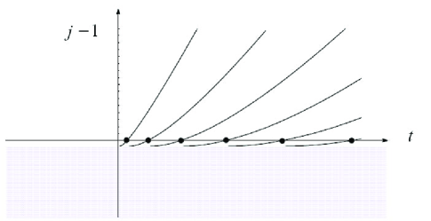
Figure 3: The $J$-plane structure for the $C=-1$ sector is schematically represented by the spectrum for hard-wall model. As $t$ decreases, trajectories move under the fixed-cut at $j=j^{(-)}_{0}$ and disappear from the physical sheet. The transition region from moving-pole to fixed cut is model-dependent. At sufficiently large $t$ each trajectory attains a fixed slope, corresponding to the tension of the model’s confining flux tubes. This $J$-plane structure for the $C=-1$ sector is similar to that for the $C=+1$ sector, as depicted in Fig. 8 of Ref. [1].

Since the metric is changed near $r_{0}$, the associated Schrödinger problem approaches the conformal limit only for $r\gg r_{0}$. However, for $-t\gg\Lambda^{2}$, it has been shown in [1] that the effective potential is insensitive to the region near $r_{0}$. This is consistent with the expectation in the QCD literature that the BFKL calculation is infrared-safe for large negative $t$, while the effects of confinement become important as $t\to 0^{-}$, and for $t>0$. For illustrative purpose, it is instructive to work with a “hard-wall” toy model. The main advantage of the hard-wall model is that it can be treated analytically. Since the metric is still $AdS_{5}\times W$, we have the same quantum mechanics problem to solve as in the conformal case except for a cutoff on the space at $r_{0}$. While this model is not a fully consistent theory, it does capture key features of confining theories with string theoretic dual descriptions. For instance, the resulting $J$-plane spectrum which exhibits a set of Regge trajectories at positive $t$ and the presence of an BFKL cut can be schematically represented by Fig. 3. We will return to these features for both $C=\pm 1$ sectors in Sec. 5.

3 Conformal Odderon Propagator in Target Space

In this section, we begin by first providing a simplified discussion for both the $C=\pm 1$ sectors based on the “ultra-local” approximation. Just like the case for the Pomeron discussed in [1], this leads to a “red-shifted” Odderon. This effective Odderon is linear for $t>0$ and is a constant near $j=1$ for $t<0$, with a kink at $t=0$. We next introduce diffusion, moving from the flat-space scattering to AdS. We will restrict ourselves to the conformal limit. By turning the problem into an equivalent Schrödinger problem, the $J$-plane singularity follows from a standard spectral analysis. In particular, in the conformal limit, the spectrum consists of a continuum, corresponding to a $J$-plane branch-cut, (1.2).

3.1 Ultra-Local Approximation

To see how Regge behavior differs in a curved-space from a flat-space, let us begin by providing an heuristic treatment. In the case of $AdS$, let us first assume that scattering takes place “locally”, i.e., only when all particles are located at the same $r$. The local inertial quantities are

$$\tilde{s}=\frac{R^{2}}{r^{2}}s\ ,\quad\tilde{t}=\frac{R^{2}}{r^{2}}t\ ,$$ (3.1)

and, with $r$ fixed, the ten-dimensional scattering process remains in the Regge regime when $s$ is sufficiently large. Thus at fixed $r$ we have, instead of (2.7) and (2.11),

$${\cal T}^{(\pm)}_{10}(\tilde{s},\tilde{t})\sim f^{(\pm)}(\alpha^{\prime}\tilde{t})(\alpha^{\prime}\tilde{s})^{\alpha_{\pm}(0)+\alpha^{\prime}\tilde{t}/2}\sim s^{\alpha_{\pm}(0)+\alpha^{\prime}_{eff}(r)t/2},$$ (3.2)

where $\alpha_{+}(0)=2$, $\alpha_{-}(0)=1$, and

$$\alpha^{\prime}_{\rm eff}(r)=\frac{R^{2}\alpha^{\prime}}{r^{2}}\;.$$ (3.3)

with $f^{(\pm)}$ process-dependent functions. We have also left out wave functions, $\{\psi_{i}(r)\}$, for four external hadrons. It follows that one arrives at scattering in 4-dim by summing over the $AdS$ radius, i.e.,

$${\cal T}^{(\pm)}_{4}(s,t)\sim\int dr\,\sqrt{-G}\,{\cal T}^{(\pm)}_{10}(\tilde{s},\tilde{t})\ ,$$ (3.4)

leading to a 4-dim Pomeron and Odderon respectively by superpositions. By examining the exponent of $s$, we see that the intercepts at $t=0$ remain at 2 and 1 respectively, just as in flat spacetime. We also see that the slope of $t$, $\alpha^{\prime}_{eff}$, depends on $r$. It is as though, in this “ultralocal” approximation, each pair of five-dimensional Pomeron and Odderon gives rise to a continuum of four-dimensional Pomerons and Odderons, one pair for each value of $r$ and each with a slope $\sim 1/r^{2}$. 

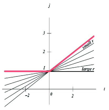
Figure 4: In the ultralocal approximation, the leading singularity for $C=-1$ (the singularity with largest $j$ at fixed $t$) is the usual linear Regge trajectory for $t>0$ but is a constant at $j=1$ for $t<0$. The ultralocal picture for $C=+1$ is identical, except for the intercept at $t=0$ shifted up to $j=2$, as illustrated by Fig. 1 of Ref. [1].

At large $s$, the highest trajectory will dominate. Recall, for the Pomeron, at positive $t$, this would be the one at the minimum value $r_{0}$:

$$\alpha^{(+)}_{eff}(t)\simeq 2+\alpha^{\prime}_{eff}(t>0)\;t\;,\quad{\rm and}\quad\alpha^{\prime}_{\rm eff}(t>0)=\frac{R^{2}\alpha^{\prime}}{r_{0}^{2}}\equiv\alpha^{\prime}_{0}\ .$$ (3.5)

For negative $t$, it would be the trajectories at large $r$. The wavefunctions in the superposition (3.4) make the integral converge at large $r$, so at any given $s$ the dominant $r$ is finite, but as $s$ increases the dominant $r$ moves slowly toward $\infty$ and so we have

$$\alpha^{\prime}_{\rm eff}(t<0)\simeq 0\ .$$ (3.6)

Same analysis also applies to the Odderon. For positive $t$, the effective Odderon sits at small $r$ and so its properties are determined by the confining dynamics. At negative $t$, the effective “spin” of an exchanged Odderon is

$$\alpha^{(-)}_{\rm eff}(t)\simeq 1+\frac{1}{2\sqrt{\lambda}}\frac{R^{4}}{r^{2}}t$$ (3.7)

The largest value sits at large $r$ and so is effectively a very small object, analogous to the tiny (and therefore perturbative) three-gluon Odderon.

This is illustrated schematically in Fig. 4. We see that, under this approximation, the dominant Odderon trajectory has a kink at $t=0$, as noted in [1] for the Pomeron.

3.2 Diffusion in AdS

However, the ultralocal approximation ignores diffusion in $AdS$. Regge behavior is intrinsically non-local in the transverse space. For flat-space scattering in 4-dimension, the transverse space is the 2-dimensional impact space, $\vec{b}$. In the Regge limit of $s$ large and $t<0$, the momentum transfer is transverse. Going to the $\vec{b}$-space,

$$t\to\nabla_{b}^{2}\;,$$ (3.8)

and the flat-space Regge propagator, for both $C=\pm 1$ sectors, is nothing but a diffusion kernel

$$\langle\;\vec{b}\;|\;(\alpha^{\prime}s)^{\alpha_{\pm}(0)+\alpha^{\prime}t/2}\;|\;\vec{b}^{\prime}\;\rangle\to(\alpha^{\prime}s)^{\alpha_{\pm}(0)}\;\frac{e^{-(\vec{b}-\vec{b}^{\prime})^{2}/(2{\alpha^{\prime}}^{2}\tau)}}{\tau^{(D-2)/2}}$$ (3.9)

with $\tau=\log(\alpha^{\prime}s)$, $\alpha_{+}(0)=2$ and $\alpha_{-}(0)=1$. Therefore, in moving to a ten-dimensional momentum transfer $\tilde{t}$, we must keep a term previously dropped, coming from the momentum transfer in the six transverse directions.

Let us first focus on $C=+1$ sector. This extra term leads to diffusion in extra-directions, i.e.,

$$\alpha^{\prime}\tilde{t}\to{\alpha^{\prime}}\Delta_{P}\equiv\frac{\alpha^{\prime}R^{2}}{r^{2}}\nabla_{b}^{2}+{\alpha^{\prime}}\Delta_{\perp P}\ .$$ (3.10)

The transverse Laplacian is proportional to $R^{-2}$, so that the added term is indeed of order ${\alpha^{\prime}}/{R^{2}}=1/\sqrt{\lambda}$. The Laplacian acts in the $t$-channel, on the product of the wavefunctions of states 1 and 2 (or 3 and 4). The subscript $P$ indicates that we must use the appropriate curved spacetime Laplacian for the Pomeron being exchanged in the $t$-channel [1]. We see that $\tilde{s}^{\alpha^{\prime}\tilde{t}/2}\sim e^{({\alpha^{\prime}}\Delta_{P}/2)\tau}$ is now a diffusion operator in all eight transverse dimensions, not just the Minkowski directions. By ignoring the $\theta$ variables, $\Delta_{\perp P}$ involves only the AdS radius r.

To obtain the $C=+1$ Regge exponents we will have to diagonalize the differential operator (3.10). Instead of an “ultralocal” Pomeron, we will have a more normal spectral problem. Using a Mellin transform, $\int_{0}^{\infty}d\tilde{s}\;{\tilde{s}}^{-j-1}$, the Regge propagator can be expressed as

$$\tilde{s}^{2+\alpha^{\prime}\tilde{t}/2}=\int\frac{dj}{2\pi i}\;\frac{{\tilde{s}}^{j}}{j-2-\alpha^{\prime}\Delta_{P}/2}$$ (3.11)

As shown in [1], $\Delta_{P}\simeq\Delta_{j}$, the tensorial Laplacian, and it is related to the scalar $AdS$ Laplacian $\Delta_{0}$ by $\Delta_{j}=r^{j}\;\Delta_{0}\;r^{-j}$. Making use of the EOM for traceless-transverse metric fluctuations, $\Delta_{2}h_{MN}=0$, it is sufficient to replace $\Delta_{j}$ by $\Delta_{2}$ for determining the first strong coupling correction, $O(1/\sqrt{\lambda})$, to the Pomeron intercept, (1.1). It is also convenient to introduced a $J$-plane $C=+1$ propagator $G^{(+)}(j)$.

$$G^{(+)}(j)=\frac{1}{j-2-\alpha^{\prime}\Delta_{2}/2}$$ (3.12)

In Ref. [1], one finds that this leads to a $J$-plane cut. We will return to this shortly.

A similar analysis can next be carried out for the $C=-1$ sector. In moving to AdS, we simply replace the Regge kernel by

$$\tilde{s}^{1+\alpha^{\prime}\tilde{t}/2}=\int\frac{dj}{2\pi i}\;{\tilde{s}}^{j}\;G^{(-)}(j)=\int\frac{dj}{2\pi i}\;\frac{{\tilde{s}}^{j}}{j-1-\alpha^{\prime}\Delta_{O}/2}$$ (3.13)

where we have again introduced a $J$-plane $C=-1$ propagator. The operator $\Delta_{O}(j)$ can be fixed by examining the EOM at $j=1$ for the associated super-gravity fluctuations responsible for this exchange, i.e., the anti-symmetric Kalb-Ramond field, $B_{MN}$. There are two classes of EOM’s:

$$(\square_{Maxwell}-(k+4)^{2})B^{(1)}_{IJ}=0\;,\quad(\square_{Maxwell}-k^{2})B^{(2)}_{IJ}=0$$ (3.14)

$k=0,1,2,\cdots$, where $\square_{Maxwell}$ stands for the Maxwell operator defined in Eq. A.2. However, for $k\neq 0$, there would be associated fluctuations on W, which we ignore, thus leaving two solutions, both for $k=0$. We also normalize the $\square_{Maxwell}$ operator so that its component in flat transverse directions is $(R^{4}/r^{2})\nabla_{b}^{2}$. For both cases, we have

$$G^{(-)}(j)=\frac{1}{j-1-(\alpha^{\prime}/2R^{2})(\square_{Maxwell}-m^{2}_{AdS,i})}$$ (3.15)

where the AdS mass-squared are 

$$m^{2}_{AdS,1}=16\;,\quad m^{2}_{AdS,2}=0\;.$$ (3.16)

We are now in position to demonstrate that (3.12) and (3.15) lead to diffusion in AdS for $C=+1$ and $C=-1$ sectors respectively. We shall treat both cases in parallel. It is convenient to switch to coordinate $z=R^{2}/r$ for the $AdS$ coordinate. Denote matrix elements by $G^{(\pm)}(z,z,^{\prime};j,t)=\langle z;t\;|G^{(\pm)}(j)|\;z^{\prime};t\rangle$, we adopt a normalization so that $(zz^{\prime})^{2}G^{(\pm)}$ each satisfies a standard $AdS_{5}$ scalar equation. Indeed, at $j=2$ and $j=1$ respectively, each reduces precisely to the equation for an $AdS_{5}$ scalar propagator, up to a constant factor $2\sqrt{\lambda}$. It is actually simpler to deal with $G^{(\pm)}$ directly, and one finds

$$(1/2\sqrt{\lambda})\left\{-z\partial_{z}z\partial_{z}+{z^{2}}t+m^{2}_{\pm}(j)\right\}G^{(\pm)}(z,z^{\prime};j,t)=z\;\delta(z-z^{\prime})$$ (3.17)

where $m^{2}_{+}(j)=2\sqrt{\lambda}(j-2)+4$ and $m^{2}_{-}(j)=2\sqrt{\lambda}(j-1)+m^{2}_{AdS,i}$. $G^{(\pm)}$ can now be found by a standard spectral analysis.

Recall that a diffusion operator resembles a Schrödinger operator in imaginary time, and the desired diagonalization can be similarly treated. To turn this into a conventional Schrödinger-like equation, introduce a new variable $u$, where $z=z_{0}e^{-u}$ and $z_{0}$ arbitrary. For simplicity, we will set $z_{0}=1$ in what follows. Aside from the $J$-dependent term $m^{2}_{\pm}(j)$, we need only to solve a standard Schrödinger eigenvalue problem, e.g.,

$$H^{(\pm)}\Psi_{E}(u)=[-\partial_{u}^{2}+V(u,t)]\Psi_{E}(u)=E\Psi_{E}(u)$$ (3.18)

with $V(u,t)=-te^{-2u}$. We can simplify the problem further by considering $t=0$ first. This has the same eigenstates as a free particle. The spectral representation  for $G^{\pm}$ at $t=0$ is

$$G^{(\pm)}(z,z^{\prime};j,0)=\frac{1}{\sqrt{\lambda}}\int_{-\infty}^{\infty}d\nu\frac{e^{2i\nu(u-u^{\prime})}}{j-j_{0}^{\pm}+{\cal D}\nu^{2}}$$ (3.19)

with $j^{(\pm)}_{0}$ given by (1.1) and (1.2), and ${\cal D}=2/\sqrt{\lambda}$.

Upon taking an inverse Mellin transform, it follows that

$$\langle z;0|\tilde{s}^{\alpha_{\pm}(0)+\alpha^{\prime}\tilde{t}/2}|z^{\prime};0\rangle=e^{j^{(\pm)}_{0}\tau}\;\frac{e^{-2(u-u^{\prime})^{2}/{\cal D}\tau}}{\sqrt{\pi{\cal D}\tau}}$$ (3.20)

where we have $\tau=\log\tilde{s}$. This is the same type of behavior found by BFKL in perturbative context. Here, it corresponds to diffusion in AdS. In particular, we can identify $j^{(\pm)}_{0}$ as the strong coupling limit of the Pomeron and Odderon intercepts respectively. Also from (3.19), one can verify that there is a branch point in the $J$-plane ending at $j^{(\pm)}_{0}$, as summarized in Table 1, for both $C=\pm 1$.

For $t\neq 0$, the eigenvalue problem can again be solved in terms of Bessel functions while the spectrum remains unchanged. Instead of (3.19), one has

$$G^{(\pm)}(z,z^{\prime};j,t)=\frac{2}{\sqrt{\lambda}\pi^{2}}\int_{-\infty}^{\infty}d\nu\;\nu\sinh 2\pi\nu\frac{K_{2i\nu}(|t|^{1/2}e^{-u})K_{-2i\nu}(|t|^{1/2}e^{-u^{\prime}})}{j-j_{0}^{\pm}+{\cal D}\nu^{2}}$$ (3.21)

Therefore, the spectrum in the $J$-plane remains a fixed cut at $j=j^{(\pm)}_{0}$.

It is also useful to explore the conformal invariance as the isometry of transverse $AdS_{3}$. As shown in [9], upon taking a two-dimensional Fourier transform with respect to $q_{\perp}$, where $t=-q_{\perp}^{2}$, one finds that $G^{(\pm)}(z,x^{\perp},z^{\prime},x^{\prime\perp};j)$ can be expressed simply as

$$G^{(\pm)}(z,x^{\perp},z^{\prime},x^{\prime\perp};j)=\frac{1}{4\pi zz^{\prime}}\frac{e^{(2-\Delta^{(\pm)}(j))\xi}}{\sinh\xi}\;.$$ (3.22)

The variable $\xi$ is related to the $AdS_{3}$ chordal distance

$$v=\frac{(x^{\perp}-x^{\prime\perp})^{2}+(z-z^{\prime})^{2}}{2zz^{\prime}}$$ (3.23)

by $\cosh\xi=1+v$, and

$$\Delta^{(\pm)}(j)=2+\sqrt{2}\;\lambda^{1/4}\sqrt{(j-j^{(\pm)}_{0})}$$ (3.24)

is a $J$-dependent effective $AdS_{5}$ conformal dimension .

For completeness, we note that, for both $C=+1$ and $C=-1$, it is useful to introduce Pomeron and Odderon kernels in a mixed-representation,

$${\cal K}^{(\pm)}(s,z,x^{\perp},z^{\prime},x^{\prime\perp})\sim\left(\frac{(zz^{\prime})^{2}}{R^{4}}\right)\int\frac{dj}{2\pi i}\;\left[\frac{(-\tilde{s})^{j}\pm(\tilde{s})^{j}}{\sin\pi j}\right]G^{(\pm)}(z,x^{\perp},z^{\prime},x^{\prime\perp};j)\;.$$ (3.25)

To obtain scattering amplitudes, we simply fold these kernels with external wave functions. Eq. (3.25) also serves as the starting point for eikonalization; we will return to this point in Sec. 6.

3.3 Conformal Geometry at High Energies

We now turn to a brief discussion on the conformal invariance of the $C=\pm 1$ kernels, $G^{(\pm)}(j)$. As pointed out in Ref. [9] the strong coupling AdS Pomeron ($C=+1$) kernel is almost completely determined by conformal symmetry or more precisely the subgroup of the conformal group that commutes with the boost operator $M_{+-}$. In the dual theory this subgroup corresponds to the $SL(2,C)$ isometries of the Euclidean $AdS_{3}$ submanifold transverse to the lightcone co-ordinates: $x^{0}\pm x^{3}$, (see Appendix B for details.) As such it plays the same role as the little group which commutes with the energy operator $P_{0}$. Here we extend this observation to the Odderon ($C=-1$) kernel.

Consider a general $n$-particle scattering amplitude, $A(p_{1},p_{2},\cdots p_{n})$. Regge exchange corresponds to having a large rapidity gap separating the $n$ particles into two sets: the right movers and left movers, with large $p^{+}_{r}=(p^{0}_{r}+p^{3}_{r})/\sqrt{2}$ and large $p^{-}_{\ell}=(p^{0}_{\ell}-p^{3}_{\ell})/\sqrt{2}$ momenta respectively [1, 9]. The $C=\pm 1$ kernels are obtained by applying this limit to the leading diagrams, in the $1/N_{c}$ expansion, that carries respective vacuum quantum numbers in the $t$-channel. The rapidity gaps, $\ln(p^{+}_{r}p^{-}_{\ell})$, between any right- and left-moving particles are all $O(\log s)$, i.e., a large Lorentz boost, $\exp[yM_{+-}]$, with $y\sim\log s$, is required to switch from the frame comoving with the left movers to the frame comoving with the right movers. Clearly, the large $y$ behavior is controlled by the leading spectrum of $M_{+-}$.

Since the $J$-plane is conjugate to rapidity, upon taking a Mellin transform, the spectrum of the boost generator $M_{+-}$ can be found by examining the resolvent, $(j-M_{+-})^{-1}$. This resolvent is nothing but the Regge propagator for $C=\pm 1$ respectively. To evaluate this propagator, we can go to a basis where $M_{+-}$ is diagonal. Since $M_{+-}$ commutes with all the generators of $SL(2,C)$, one finds that the propagator $(j-M_{+-})^{-1}$ can be expressed in terms of $SL(2,C)$ Casimirs.

From a more intuitive perspective, one recognizes that high energy small-angle scattering can be separated into longitudinal and transverse, relative to the momentum direction of the incoming particles. The transverse subspace of $AdS_{5}$ is $AdS_{3}$. It is therefore not surprising to find that the co-ordinate representation for both the $C=\pm 1$ Regge propagators can be expressed as bulk-to-bulk scalar propagators in the transverse Euclidean $AdS_{3}$ with $SL(2,C)$ isometries. Very likely this is a generic property in all conformal gauge theories.

In Appendix B, we briefly review how $SL(2,C)$ generator algebra can be realized on $AdS_{3}$. In general, unitary representations of $SL(2,C)$ are labeled by $h=i\nu+(1+n)/2$, and $\bar{h}=i\nu+(1-n)/2$, which are the eigenvalues for the highest-weight state of $J_{0}$ and $\bar{J}_{0}$. The principal series is given by real $\nu$ and integer $n$. For our leading order strong coupling Pomeron and Odderon, one finds that $J^{2}=\bar{J}^{2}=-(1/4+\nu^{2})$; we are thus restricted to $n=h-\bar{h}=0$ and are insensitive to rotations in the impact parameter plane by $M_{12}$.

Let us focus here on the $C=-1$ sector. To leading order in strong coupling, the boost operator can be expressed as $M_{+-}=1-H^{(-)}_{+-}/(2\sqrt{\lambda})+O(1/\lambda)$, with $H^{(-)}_{+-}$ given by the DE obeyed by the propagator $G^{(-)}$, or equivalently, $zz^{\prime}G^{(-)}$, i.e., Eq. (B.4). From (B.7), we find

$$H^{(-)}_{+-}=-z^{3}\partial_{z}z^{-1}\partial_{z}-z^{2}\nabla^{2}_{x_{\perp}}+m^{2}_{AdS}-1=-2J^{2}-2\bar{J}^{2}+m^{2}_{AdS}-1\;.$$ (3.26)

After a similarity transformation, $H^{(-)}_{+-}$ can be diagonalized by a Fourier transform, with eigenvalue $-\infty<\nu<\infty$ and eigenfunction

$$Y_{\nu}(v)=\frac{1}{4\pi}\frac{e^{2i\nu\xi}}{\sinh\xi}\;.$$ (3.27)

It follows that the boost operator $M_{+-}$ is diagonal in the $\nu$-basis and, in the strong coupling,

$$M_{+-}\rightarrow j^{(-)}(\nu)=j^{(-)}_{0}-{\cal D}\nu^{2}+0(\nu^{4})\;.$$ (3.28)

with $j^{(-)}_{0}=1-m^{2}_{AdS}/\sqrt{\lambda}$ and ${\cal D}=2/\sqrt{\lambda}$.

We are now in the position to put everything together, for both $C=+1$ and $C=-1$. It is useful to introduce Pomeron and Odderon propagators in a mixed-representation,

$$\left(\frac{1}{zz^{\prime}}\right)\int\frac{d\nu}{\pi}\;\frac{1}{j-j^{(\pm)}_{0}+{\cal D}\nu^{2}}{Y}_{\nu}(v)\;.$$ (3.29)

Closing the $\nu$-contour, one obtains $G^{(\pm)}(z,x^{\perp},z^{\prime},x^{\prime\perp};j)$, given by Eq. (3.22).

It is interesting to note that this strong coupling Hamiltonian structure, (3.26), is similar to the weak coupling one-loop $n_{g}$ gluon BFKL spin chain operator in the large $N_{c}$ limit. Here the boost operator is approximated by $M_{+-}=1-(\alpha N_{c}/\pi)H_{\rm BFKL}$, where

$$H_{\rm BFKL}=\frac{1}{4}\sum^{n_{g}}_{i=1}[{\cal H}(J^{2}_{i,i+1})+{\cal H}(\bar{J}^{2}_{i,i+1})],$$ (3.30)

is a sum over two-body operators with holomorphic and anti-holomorphic functions of the Casimir. The Yang-Mills coupling is defined as $\alpha=g^{2}_{YM}/4\pi$. Even numbers of gluons ($n_{g}$) contribute to the BFKL Pomeron with charge conjugations $C=+1$ and odd number of gluons to the weak coupling Odderon [22, 24, 25, 26] with charge conjugations $C=-1$. More discussion on the relation between the strong-coupling and weak-coupling limits can be found in [9].

4 Odderon Vertex on the World-Sheet

It has been demonstrated in Ref. [1] that Regge behavior for string scattering in flat-space follows from an OPE on world-sheet. Since the flat space (super) string is integrable with an explicit closed form for the amplitude, it is possible to define in closed form the on-shell Reggeon vertex. For example the on-shell Pomeron vertex is given by

$${\cal V}_{P}^{\pm}=(2\partial X^{\pm}\bar{\partial}X^{\pm}/\alpha^{\prime})^{1+\alpha^{\prime}t/4}e^{\mp ik\cdot X}\;.$$ (4.1)

(See [42] for a related discussion.) This operator (and a similar Reggeized gauge field operator for the open string) enables a very elegant direct evaluation of Regge and multi-Regge amplitudes reproducing all the results in the early literature, for example as reviewed in Ref. [43] for the open string.

In $AdS_{5}\times S^{5}$, without a closed form solution for amplitudes, no closed form particle or Regge vertex operator has been constructed. However Ref. [1] did succeed in finding the Pomeron vertex to leading order in the strong coupling approximation. A key step involves in identifying the Pomeron source as a generalized (1,1) conformal worldsheet vertex operator, satisfying the on-shell conditions: $L_{0}=\bar{L}_{0}=1$. Here we will generalized this analysis for the Odderon.

We begin by treating the bosonic sector of the supergravition multiplet in flat space introduce in Sec. 2.2, Eq. (2.10). The natural guess is take the high energy limit for a more general Reggeon operator insertion,

$${\cal V}(T)=(T_{MN}\partial X^{M}\bar{\partial}X^{N}/\alpha^{\prime})^{1+\alpha^{\prime}t/4}e^{\mp ik\cdot X}\;,$$ (4.2)

where one can expand ${\cal V}(T)$ into a leading symmetric traceless ($h_{MN}$), antisymmetric ($B_{MN}$) and the trace ($\phi\;\eta_{MN}$) contributions, appropriate for the Pomeron, Odderon and dilaton respectively. Generalization to the entire supergravity multiplet including the Fermionic fields is straight forward in principle but truncating to bosonic degrees of freedom has the advantage of being able drop all world sheet Grassmann variable from the outset.

4.1 Pomeron/Odderon Vertex Operator in Flatland

One of the key observation made in [1] is the recognition that Regge behavior in flat-space scattering follows also directly from the world sheet OPE. For instance, for the standard bosonic closed string scattering involving 4 external tachyons, the amplitude is given by

$$A_{4} = \intop d^{2}w\;\langle e^{ip_{1}\cdot X(0)}e^{ip_{2}\cdot X(w,\bar{w})}e^{ip_{3}\cdot X(1)}e^{ip_{4}\cdot X(\infty)}\rangle$$ (4.3)

$$= \intop d^{2}w\;|w|^{-4-\alpha^{\prime}t/2}|1-w|^{-4-\alpha^{\prime}s/2}$$

In the Regge limit, defined by $|s|\rightarrow\infty$ along the positive imaginary axis, the second factor can be approximated by $|1-w|^{-4-\alpha^{\prime}s/2}\sim e^{\alpha^{\prime}s(w+\bar{w})/4}$, leading to a cutoff, $|w|=O(1/s)$. This is equivalent to keeping the first non-trivial term,

$$e^{\textstyle ip_{1}\cdot X(0)}e^{\textstyle ip_{2}\cdot X(w,\bar{w})}\sim|w|^{\textstyle-4-\alpha^{\prime}t/2}\;e^{\textstyle ik\cdot X(0)+ip_{2}\cdot(w\partial+\bar{w}\cdot\bar{\partial})X(0)}\;,$$ (4.4)

in the OPE. Regge behavior then follows,

$$\int d^{2}w|w|^{-4-\alpha^{\prime}t/2}e^{\alpha^{\prime}s(w+\bar{w})/4}=\Pi(\alpha(t))\;s^{\alpha(t)}\;,$$ (4.5)

where

$$\Pi(\alpha(t))=2\pi\frac{\Gamma(-\alpha(t)/2)}{\Gamma(1+\alpha(t)/2)}e^{-i\pi\alpha(t)/2}\sim\frac{e^{-i\pi\alpha(t)}+1}{\sin\pi\alpha(t)}\ ,$$ (4.6)

and $\alpha(t)=2+\alpha^{\prime}t/2$.

We note that the terms $\partial X_{M}(0)$ and $\bar{\partial}X_{N}(0)$ in (4.4) single out the level-one oscillators, $a^{\dagger}_{1,M}$ and $\tilde{a}^{\dagger}_{1,N}$ that contribute to states on the leading Regge trajectory. We also note that, with (4.6), Eq. (4.5) can be expressed as (2.7), appropriate for an $C=+1$ exchange.

To generalize this to the $C=-1$ sector we must go beyond elastic tachyon amplitude. Due to symmetry under crossing, $s\leftrightarrow u$, only $C=+1$ states, which are even under worldsheet parity, couple in the t-channel. The odd sector couples first in the four point amplitude involving two external $C=-1$ states, one initial and one final in the t-channel. This is due to world-sheet parity conservation. It is also useful to consider the general case of scattering involving an arbitrary number of external particles of different types. The amplitude can be calculated at the tree-level as an integral

$$A_{n}=\intop d^{2}w_{2}d^{2}w_{3}\cdots d^{2}w_{n-2}<V_{1}V_{2}\cdots V_{N}>.$$ (4.7)

where $V_{i}$ are the corresponding vertex operators, including that for $C=-1$ states. (Here, we have also made use of Möbius invariance to fix three points, i.e., $w_{1}$, $w_{n-1}$ and $w_{n}$.) In the Regge limit, one factorizes this into left- and right-moving, denoted by ${\cal W}_{R}$ and ${\cal W}_{L}$ for sets of $l_{R}$ right-moving and $l_{L}$ left-moving vertex operators together with their associated $l_{R}-2$ and $l_{L}-2$ world-sheet integrations.

$$A_{n}=\int d^{2}w\left\langle{\cal W}_{R}w^{L_{0}-2}\bar{w}^{\bar{L}_{0}-2}{\cal W}_{L}\right\rangle\ .$$ (4.8)

Integrating over $\int d^{2}w$ leads to level matching conditions $L_{0}=\bar{L}_{0}$ and the string propagator $(L_{0}+\bar{L}_{0}-2)^{-1}$. It was also demonstrated in [1] that the leading Regge behavior corresponds to satisfying the J-plane constraint,

$$L_{0}(j,t)=\bar{L}_{0}(j,t)=j/2-\alpha^{\prime}t/4=1,\quad{\rm or}\quad j=2+\alpha^{\prime}t/2\;.$$ (4.9)

which interpolates through the physical states on the leading trajectory. Taken together these constraints can be represented by an inverse Mellin transform,

$$A_{n}\simeq\int\frac{dj}{2\pi i}\frac{{\cal F}(j)\;\delta_{L_{0},\tilde{L}_{0}}}{L_{0}(j,t)+\tilde{L}_{0}(j,t)-2}\;.$$ (4.10)

The residue is evaluated by the insertion of Reggeon vertex operator and the integral performed by contour integration over the pole at $j=2+\alpha^{\prime}t/2$. For example in the Pomeron case the result [1] was $A_{n}\sim\Pi(\alpha(t))\left\langle{\cal W}_{R}\,{\cal V}_{P}^{-}\right\rangle\left\langle{\cal V}_{P}^{+}\,{\cal W}_{L}\right\rangle$, or more explicitly by a large relative boost, $exp[-yM_{+-}]$, for the states ${\cal W}_{L}$ and ${\cal W}_{R}$ back to their approximate rest frames (denoted by a subscript 0),

$$A_{n}\sim\Pi(\alpha(t))(s/s_{0})^{2+\alpha^{\prime}t/2}\left\langle{\cal W}_{R0}\,{\cal V}_{P}^{-}\right\rangle\left\langle{\cal V}_{P}^{+}\,{\cal W}_{L0}\right\rangle\;.$$ (4.11)

where the large boost parameter (or rapidity gap) is $y=\log(s/s_{0})$. The result (4.11) has a simple interpretation as a Pomeron propagator, $(s/s_{0})^{2+\alpha^{\prime}t/2}$, times the couplings of the Pomeron to the two sets of vertex operators. To clarify this consider again the simple case of the 4-point function at $t=0$. In this case, one needs only to evaluate the following 3-point function,

$$\langle e^{ip_{1}\cdot X(1)}e^{ip_{2}\cdot X(2)}e^{\mp ik\cdot X(w,\bar{w})}(h_{MN}\partial X^{M}\bar{\partial}X^{N}/\alpha^{\prime})\rangle\;,$$ (4.12)

where $k=p_{1}+p_{2}$ and $k\cdot(p_{1}-p_{2})=0$. Note that this is analogous to a graviton-tachyon-tachyon coupling vertex. In CM, and using LC coordinates, $p_{1,2}$ have large $``+"$ components, $O(\sqrt{s})$, if they are R-moving, and large $``-"$ components, if they are L-moving. The corresponding small components are $O(1/\sqrt{s})$, and components orthogonal to $\pm$ are $O(1)$. From the commutation relations, $[a_{1}^{\pm},{a^{\mp}_{1}}^{\dagger}]=\pm 1$, the dominant contribution at large $s$ comes from $h_{-,-}$ (for R-moving) and $h_{+,+}$ (for L-moving), leading to the dominant LC components, (4.1). The analysis above holds also for $t\neq 0$ and can be carried out for general n-point amplitudes, leading to (4.11).

Returning to the general case insert the operator,

$${\cal V}(T)=(T_{MN}\partial X^{M}\bar{\partial}X^{N}/\alpha^{\prime})^{1+\alpha^{\prime}t/4}e^{\mp ik\cdot X}$$ (4.13)

and factorize the tensor and take the high energy limit. The leading term on-shell at $t=0$ defines 3 vertex operators:

$$\langle{\cal W}_{R}\;e^{ikX}h_{MN}\partial X^{M}\overline{\partial}X^{N}\rangle \simeq \langle{\cal W}_{R}\;e^{ikX}h_{--}\partial X^{-}\overline{\partial}X^{-}\rangle=O(s)\;,$$

$$\langle{\cal W}_{R}\;e^{ikX}B_{MN}\partial X^{M}\overline{\partial}X^{N}\rangle \simeq \langle{\cal W}_{R}\;e^{ikX}B_{-\perp}(\partial X^{-}\overline{\partial}X^{\perp}-\partial X^{\perp}\overline{\partial}X^{-})\rangle=O(\sqrt{s})\;,$$

$$\langle{\cal W}_{R}\;e^{ikX}\eta_{MN}\partial X^{M}\overline{\partial}X^{N}\rangle \simeq O(1)\;.$$ (4.14)

For $t\neq 0$ the leading term picks up a common factor of $(\partial X^{-}\bar{\partial}X^{-})^{\frac{\alpha^{\prime}t}{4}}$ on the left,

$$[(h_{MN} + B_{MN})\partial X^{M}\overline{\partial}X^{N}]^{1+\frac{\alpha^{\prime}t}{4}}$$

$$\simeq \left[h_{--}(\partial X^{-}\overline{\partial}X^{-})+B_{-\perp}(\partial X^{-}\overline{\partial}X^{\bot}-\partial X^{\perp}\overline{\partial}X^{-})\right](\partial X^{-}\overline{\partial}X^{-})^{\frac{\alpha^{\prime}t}{4}}\;.$$

For ${\cal W}_{L}$, we need to replace $X^{-}$ by $X^{+}$, with a common factor $(\partial X^{+}\bar{\partial}X^{+})^{\frac{\alpha^{\prime}t}{4}}$ on the right. When they are combined, the symmetric combination, i.e., the first term above, leads to the Pomeron vertex operator. The anti-symmetric combination, the second term, contributing to $1/s$ down relative to the first term, corresponds to an Odderon exchange.

In analogy with ${\cal V}_{P}^{\pm}$, we can now define an Odderon vertex operator

$${\cal V}_{O}^{\pm}=(2\epsilon_{\pm,\perp}\partial X^{\pm}\bar{\partial}X^{\perp}/\alpha^{\prime})(2\partial X^{\pm}\bar{\partial}X^{\pm}/\alpha^{\prime})^{\alpha^{\prime}t/4}e^{\mp ik\cdot X}$$ (4.16)

which characterizes the exchange of a leading Odderon. Here $\epsilon_{\pm,\perp}=-\epsilon_{\perp,\pm}$. Just as for the Pomeron, this is an on-shell vertex operator, satisfying the on-shell conditions

$$L_{0}{\cal V}^{\pm}_{O}=\bar{L}_{0}{\cal V}^{\pm}_{O}={\cal V}^{\pm}_{O}$$ (4.17)

In particular, this leading Regge trajectory interpolates those states created by level-one oscillators, $a_{1,M}^{\dagger}$ and $\tilde{a}_{1,M}^{\dagger}$, with $j=2n+1$, $t_{n}=4n\;{\alpha^{\prime}}^{-1}$, $n=0,1,\cdots$, and can be characterized by an Odderon trajectory

$$\alpha^{(-)}(t)=1+\alpha^{\prime}t/2\;,\quad{\rm or}\quad L_{0}(j,t)=\bar{L}_{0}(j,t)=(j+1)/2-\alpha^{\prime}t/4=1$$ (4.18)

Again we may boost the states back to their rest frame,

$$A_{n}\sim\Pi_{-}(\alpha^{(-)}(t))(s/s_{0})^{\alpha^{(-)}(t)}\left\langle{\cal W}_{R0}\,{\cal V}_{O}^{-}\right\rangle\left\langle{\cal V}_{O}^{+}\,{\cal W}_{L0}\right\rangle\;.$$ (4.19)

to explicitly obtain the Odderon Regge amplitude. Here, $\Pi_{-}(\alpha)=\Pi(\alpha+1)$, and (4.19) is of the form (2.11), appropriate for an crossing-odd exchange.

Let us next briefly comment on the the couplings of the Odderon, i.e., $\langle{\cal W}_{R0}\,{\cal V}_{O}^{-}\rangle$ and $\left\langle{\cal V}_{O}^{+}\,{\cal W}_{L0}\right\rangle$. Note that ${\cal V}_{P}$ and ${\cal V}_{O}$ have opposite symmetry under $\partial\leftrightarrow\bar{\partial}$, even and odd for ${\cal V}_{P}$ and ${\cal V}_{O}$ respectively. For oriented closed strings, the theory should be invariant under $w\leftrightarrow\bar{w}$. It follows that non-vanishing coupling $\langle{\cal W}_{R}\,{\cal V}_{O}^{-}\rangle$ and $\langle{\cal W}_{L}\,{\cal V}_{O}^{+}\rangle$ would require ${\cal W}_{R,L}$ to be odd under $w\leftrightarrow\bar{w}$. For example, tachyon and graviton vertex operators $V_{t}$ and $V_{g}$ are even under $w\leftrightarrow\bar{w}$. It follows that couplings involving n-tachyons and an Odderon vanish. To be precise, $\langle{\cal W}_{R}\,{\cal V}_{O}^{-}\rangle$ and $\langle{\cal W}_{L}\,{\cal V}_{O}^{+}\rangle$ are non-zero only if ${\cal W}_{R,L}$ are odd under $w\leftrightarrow\bar{w}$. Conversely, $\langle{\cal W}_{R}\,{\cal V}_{P}^{-}\rangle$ and $\langle{\cal W}_{L}\,{\cal V}_{P}^{+}\rangle$ are non-zero only if ${\cal W}_{R,L}$ are even under $w\leftrightarrow\bar{w}$. It is worth mentioning that our discussion for the Pomeron and Odderon vertex operators also apply to couplings with branes, which can be used to model “mesons”. It should also apply in the case of baryons. One can also generalize to the Fermionic sector, as discussed briefly in [1].

4.2 Pomeron and Odderon in AdS

We next extend the flat-space results to the case of an $AdS$ background. We will focus on $AdS_{5}$ without confinement deformation. In the limit of large $\lambda$, ($\lambda\equiv{R^{4}}/{\alpha^{\prime 2}}$), the world sheet path integral will be Gaussian. As emphasized in [1] for the Pomeron, we need to generalize the vertex operator to include a string wave function in $AdS$. In enforcing the on-shell condition, we must diagonalize $L_{0}$ and $\tilde{L}_{0}$ by going to a basis of definite spin. As we demonstrate below, making use of the analysis in Sec. 3.2, a complete diagonalization can be carried out.

For the $C=+1$ sector, let us begin by considering the vertex operator in a definite spin basis to have the form

$$V_{P}(j,\pm)=(\partial X^{\pm}\overline{\partial}X^{\pm})^{\frac{j}{2}}e^{\mp ik\cdot X}\phi_{\pm j}(r).$$ (4.20)

From the physical state conditions, $L_{0}V_{P}(j,\pm)=\tilde{L}_{0}V_{P}(j,\pm)=V_{P}(j,\pm)$, one has, up to $O(1/\sqrt{\lambda})$ corrections, $[\frac{j-2}{2}-\frac{\alpha^{\prime}}{4}\triangle_{j}]e^{\mp ik\cdot X}\phi_{\pm j}(Y)=0$. The on-shell condition can again be expressed in terms of a Mellin transform,

$$\int\frac{dj}{2\pi i}\frac{\delta_{L_{0},\tilde{L}_{0}}}{L_{0}(j)+\bar{L}_{0}(j)-2}\;.$$ (4.21)

It is convenient to first perform a similarity transformation, $(r/R)^{(j-2)}[L_{0}(j)+\bar{L}_{0}(j)-2]^{-1}(r/R)^{-(j-2)}$, leading to the $J$-plane Pomeron kernel is

$$G^{(+)}(j)=\frac{1}{j-2-({R^{2}}/{2\sqrt{\lambda}})\Delta_{2}}\;,$$ (4.22)

and we have replaced $\alpha^{\prime}$ by $R^{2}/\sqrt{\lambda}$. Note that this is precisely the Pomeron propagator introduced earlier, (3.12), by a diffusion consideration.

As shown in Sec. (3.2), $\Delta_{2}$ can be diagonalized using the $u$-basis, with the introduction of another continuous quantum number $\nu$. In this basis, $\phi_{+j}\sim e^{(j-2)u}K_{2i\nu}(|t|^{1/2}e^{-u})\;,$ ${\cal D}=2/\sqrt{\lambda}$, and the Pomeron vertex operator takes on the form

$${\cal V}_{P}(j,\nu,k,\pm)\sim(\partial X^{\pm}\overline{\partial}X^{\pm})^{\frac{j}{2}}e^{\mp ik\cdot X}e^{(j-2)u}K_{\pm 2i\nu}(|t|^{1/2}e^{-u})\;.$$ (4.23)

(More discussion for these solutions can be found in [1].) Following next the same steps done for the flat space, e.g., boosting back to the respective rest frames of $L$- and $R$-moving particles, we arrive at, for $C=+1$,

$${\cal T}^{(+)} \sim \int\frac{dj}{2\pi i}\int\frac{d\nu\nu\sinh{2\pi\nu}}{\pi}\frac{\Pi(j)\;s^{j}}{j-j_{0}^{(+)}+{\cal D}\nu^{2}}\left\langle{\cal W}_{R0}\,{\cal V}_{P}(j,\nu,k,-)\right\rangle\left\langle{\cal V}_{P}(j,\nu,k,+){\cal W}_{L0}\right\rangle,$$

where $\Pi(j)$ leads to a signature factor, appropriate for ${\cal T}^{(+)}$ being even in $s$. Closing the contour at $\nu=i\lambda^{1/4}\sqrt{(j-j_{0}^{(+)})/2}$ directly leads to the desired final result obtained in [1].

We are now in the position to generalize to the case of Odderon by following the same steps. Going to the $J$-plane, we introduce a vertex operator

$${\cal V}_{O}(j,\pm)=(\partial X^{\pm}\overline{\partial}X^{\perp}-\partial X^{\perp}\overline{\partial}X^{\pm})(\partial X^{\pm}\overline{\partial}X^{\pm})^{\frac{j-1}{2}}e^{\mp ik\cdot X}\phi_{\pm j\perp}(r).$$ (4.25)

The physical state condition, $L_{0}V^{\pm}_{O}(j)=\tilde{L}_{0}V^{\pm}_{O}(j)=V^{\pm}_{O}(j)$, will then give us

$$[\frac{j+1}{2}-\frac{\alpha^{\prime}}{4}\Delta_{O,j}]\phi_{\pm j\bot}(r)=\phi_{\pm j\bot}(r).$$ (4.26)

We can again perform a similarity transformation, $\phi_{\pm j\perp}=(r/R)^{(j-1)}\phi_{\pm,\perp}$, and arrive at a $J$-plane Odderon propagator,

$$G^{(-)}(j)=\frac{1}{j-1-({R^{2}}/{2\sqrt{\lambda}})\Delta_{O,1}}\;,$$ (4.27)

where $\Delta_{O,j}=(r/R)^{-(j-1)}(\Delta_{O,1})(r/R)^{(j-1)}$. To determine the diffusion operator for Odderon, $\Delta_{O,1}$, we can match the EOM at $j=1$, appropriate in the infinite $\lambda$ limit.

The EOM in this case involves a Maxwell operator, and in general will also involve an AdS mass. Both the Maxwell operator and the AdS mass squared, $m_{AdS}^{2}$, can be fixed by a proper identification of the $B_{\mu\nu}$ state of string theory at $j=1$ using the $AdS/CFT$ dictionary [33]. In [44, 33] it was found that a 2-form fields in AdS space has two solutions, corresponding to $m_{AdS}^{2}=16$ and $m_{AdS}^{2}=0$.

As done for the Pomeron, to $O(1/{\sqrt{\lambda}})$, after writing out the Maxwell operator, we have, for $z\neq z^{\prime}$, and for $j\simeq 1$, $G^{(-)}(j)$ satisfies the $C=-1$ part of Eq. (3.17). Again, the wave function, $\phi_{\pm\perp}$, satisfies the same DE. Changing variable to $u=-\ln(z/z_{0})$, we get

$$[j-1-\frac{\alpha^{\prime}t}{2}e^{-2u}-\frac{1}{2\sqrt{\lambda}}(\partial_{u}^{2}-m_{AdS}^{2})]\phi_{\pm\bot}(u)=0.$$ (4.28)

This equation can again be diagonalized by $\nu$, with

$$\phi_{+j\perp}\sim e^{(j-1)u}K_{2i\nu}(|t|^{1/2}e^{-u})\;,\quad{\rm and}\quad G^{(-)}(j)=\frac{1}{j-j_{0}^{(-)}+{\cal D}\nu^{2}}\;.$$ (4.29)

where $j_{0}^{(-)}=1-m^{2}_{i}/2\sqrt{\lambda}$, Eq. (1.2). In this basis, the Odderon vertex operator takes on the form

$${\cal V}_{O}(j,\nu,k,\pm)\sim(\partial X^{\pm}\overline{\partial}X^{\perp}-\partial X^{\perp}\overline{\partial}X^{\pm})(\partial X^{\pm}\overline{\partial}X^{\pm})^{\frac{j-1}{2}}e^{\mp ik\cdot X}e^{(j-1)u}K_{\pm 2i\nu}(|t|^{1/2}e^{-u})$$ (4.30)

Following the same steps done for $C=+1$, we arrive at

$${\cal T}^{(-)} \sim \int\frac{dj}{2\pi i}\int\frac{d\nu\nu\sinh{2\pi\nu}}{\pi}\frac{\Pi_{-}(j)\;s^{j}}{j-j_{0}^{(-)}+{\cal D}\nu^{2}}\left\langle{\cal W}_{R0}\,{\cal V}_{O}(j,\nu,k,-)\right\rangle\left\langle{\cal V}_{O}(j,\nu,k,+)\,{\cal W}_{L0}\right\rangle$$

where we again have a signature factor appropriate for amplitude being odd in s. Closing the contour at $\nu=i\lambda^{1/4}\sqrt{(j-j_{0}^{(+)})/2}$ directly leads to the desired final result.

Recall that there are two solutions for the conformal Odderon. For $m^{2}_{AdS}=16$,

$$j^{(-)}_{0,(1)}=1-8/\sqrt{\lambda}+O(1/\lambda)\;,$$ (4.32)

and, for $m^{2}_{AdS}=0$,

$$j^{(-)}_{0,(2)}=1+O(1/\lambda)\;,$$ (4.33)

as summarized in Table 1.

4.3 Conformal Dimensions, and BFKL/DGLAP Connection

We end this section with a brief discussion on the quantity $\Delta^{(\pm)}(j)$, defined in Eq. (3.24), which sets the dimension $\Delta$ as a function of Lorentz spin $J_{Lorentz}$ for the BFKL/DGLAP operators for $C=\pm 1$ sector respectively. This connection was first emphasized in Ref. [1]. The analytic continuation from DGLAP to BFKL operators has been discussed at weak coupling for some time [45, 46, 47, 48]. Recently, it was conjectured to be exact at weak coupling in ${\cal N}=4$ Yang-Mills theory [10]. The demonstration of this relationship in all large-$\lambda$ conformal theories, and the derivation of the formula for $\Delta^{(+)}(j)$, is given in section 3 of [1], where the existence of the single function $\Delta^{(+)}(j)$ with $j=j^{(+)}_{0}$ at $\Delta=2$ (the BFKL exponent) and $j=2$ at $\Delta=4$ (for the energy-momentum tensor, the first DGLAP operator) was demonstrated.

The AdS/CFT dictionary relates string states to local operators in the gauge theory. This can be summarized by the statement that gauge theory correlators can be found, in the strong coupling, by behavior of bulk (gravity) fields, $\phi_{i}(x,z)$, as they approach the $AdS_{5}$ boundary, $z\rightarrow 0$,

$$\langle e^{\int d^{4}x\phi_{i}(x){\cal O}_{i}(x)}\rangle_{CFT}={\cal Z}_{string}\left[\phi_{i}(x,z)|_{z\sim 0}\rightarrow\phi_{i}(x)\right]\;,$$ (4.34)

where $z>0$ extends into the $AdS$ bulk and the left hand side is the generating function of correlation functions in the gauge theory for the operator ${\cal O}_{i}$. For instance, in the case where $\phi(x,z)$ is the dilaton field in the bulk, it is well-known that the corresponding gauge theory operator ${\cal O}$ is $TrF^{2}$.

Let us next consider the diagonalized Pomeron and Odderon vertex operators. For simplicity, we consider the $t=0$ limit, where they become:

$${\cal V}_{P}(j,\nu,0,\pm) \sim (\partial X^{\pm}\overline{\partial}X^{\pm})^{\frac{j}{2}}e^{(j-2\pm 2i\nu)u}$$ (4.35)

$${\cal V}_{O}(j,\nu,0,\pm) \sim (\partial X^{\pm}\overline{\partial}X^{\perp}-\partial X^{\perp}\overline{\partial}X^{\pm})(\partial X^{\pm}\overline{\partial}X^{\pm})^{\frac{j-1}{2}}e^{(j-1\pm 2i\nu)u}$$ (4.36)

These vertex operators for integer $j\geq 2$ and $j\geq 1$ respectively correspond to the lightest string states of given spin, and so are dual to the lowest dimension operators of those spins. Therefore, in the large $\lambda$ limit, the physical state conditions, $L_{0}=\tilde{L}_{0}=1$, would determine the dimensions of the leading twist operators. Let us examine the Pomeron and the Odderon vertex operators from this perspective.

For $C=+1$, ${\cal V}_{P}$ at the AdS boundary will couple to a gauge invariant operator ${\cal O}^{(+)}$, i.e.,

$$\int d^{4}x\;{\cal O}^{(+)}\;{\cal V}_{P}$$ (4.37)

where ${\cal O}^{(+)}$ is an operator of dimension $\Delta^{(+)}$ and Lorentz spin $J_{L}$. By examining the number of Lorentz indices, we have $J_{L}=j$. At $j=2$, ${\cal V}_{P}$ couples to the energy-momentum tensor, whose gauge part is $tr(F_{+\mu}F_{+}^{\mu})$. For general $j$, as a leading twist operator, its gauge part is $tr(F_{+\mu}D_{+}^{J_{L}-2}F_{+}^{\mu})$, with the twist given by

$$\tau^{(+)}=\Delta^{(+)}-J_{L}$$ (4.38)

At $j=2$, $\Delta^{(+)}(2)=4$, corresponding to twist two. Due to energy-momentum conservation, anomalous dimension vanishes there, as expected.

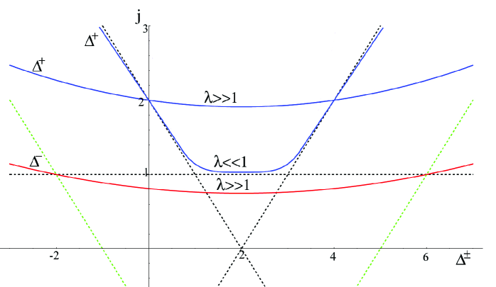
Figure 5: Schematic form of the $\Delta^{(\pm)}-j$ curves. For $C=+1$, we show in blue the curves ($\Delta^{(+)}$) for both the limit $\lambda\gg 1$ and $\lambda\ll 1$. (Fig. 2 of Ref. [1].) The curve for $C=-1$ ($\Delta^{(-)}$) at $\lambda\gg 1$ is shown in red, for the branch $m^{2}_{AdS}=16$. The dashed lines show the $\lambda=0$ DGLAP branch (slope 1), BFKL branch (slope 0), and inverted DGLAP branch (slope $-1$) for both $C=\pm 1$. Note that the $C=+1$ curves pass through the points (4,2) and (0,2) where the anomalous dimension must vanish. For $C=-1$, the curve pass through the points (6,1) and (-2,1). The inversion symmetry $\Delta\to 4-\Delta$ is shown explicitly. Note also that, Lorentz spin and $SO(3)$ spin are related by $J_{L}=j$ and $J_{L}=j+1$ for $C=+1$ and $C=-1$ respectively.

To determine $\Delta^{(+)}(j)$, let us first examine the scale transformation for ${\cal V}_{P}$. Under scale transformation, if $\delta u\sim\epsilon$, then $\delta X\sim-\epsilon X$. If $\phi_{j+}\sim e^{\zeta u}$, $\zeta=j-2+2i\nu$, it follows ${\cal V}^{+}_{P}$ scales with a dimension $2-2i\nu$. Therefore 

$$\Delta^{(+)}=4-(2-2i\nu)=2+2i\nu$$ (4.39)

On the other hand, from

$$j=j_{0}^{(+)}-{\cal D}\nu^{2}$$ (4.40)

one has

$$\Delta^{(+)}(j)=2+\sqrt{2}\;\lambda^{1/4}\sqrt{j-j_{0}^{(+)}}$$ (4.41)

or

$$j=j_{0}^{(+)}+(1/2\sqrt{\lambda})(\Delta^{(+)}-2)^{2}$$ (4.42)

as depicted in Fig. 5. As noted earlier, $\Delta=4$ for $J_{L}=j=2$, due to energy-momentum conservation. Note also that the the curve is symmetric in $\Delta\leftrightarrow 4-\Delta$, reflecting inversion symmetry in $AdS_{5}$. The intercept for the conformal Pomeron can be read off as the minimum $j$-value at $\Delta=2$. (See Table 1.)

We can repeat the same step for $C=-1$. One again arrives at

$$\Delta^{(-)}=2+2i\nu$$ (4.43)

The corresponding $\Delta-j$ curve is

$$j=j_{0}^{(-)}+(1/2\sqrt{\lambda})(\Delta^{(-)}-2)^{2}$$ (4.44)

or

$$\Delta^{(-)}(j)=2+\sqrt{2}\;\lambda^{1/4}\;\sqrt{j-j_{0}^{(-)}}$$ (4.45)

Note that the curve is again symmetric about $\Delta^{(-)}=2$. The Odderon intercept can again be read off as the minimum $J$-value at $\Delta^{(-)}=2$. We also note, at $j=1$, ${\cal V}_{O}$ has Lorentz spin 2, $J_{L}=2$, thus $j=J_{L}-1$.

There are now two branches. Consider first the branch where $m^{2}_{AdS}=16$. At $j=1$, one has $\Delta^{(-)}=6$. With Lorentz spin 2, it follows that this corresponds to a twist-4 operator, whose gauge component can be identified with $tr(F_{+\perp}F^{2})$. Due to charge conservation, anomalous dimension again vanishes there. For general $J_{L}$, ($J_{L}=j+1$), ${\cal V}_{O}$ couples to $tr(F_{+\perp}D_{+}^{j-1}F^{2})=tr(F_{+\perp}D_{+}^{J_{L}-2}F^{2})$. For $\lambda\neq\infty$, operator mixing naturally leads to the curve shown in Fig. 5, with $j_{0}^{(-)}<1$, consistent with that found in the weak coupling. For the branch $m^{2}_{AdS}=0$, we have $\Delta^{(-)}=2$ at $j=1$, and it would be interesting to identify the corresponding gauge invariant operators ${\cal V}_{O}$ for various integral $j$ values.

5 Effects of Confinement in the Hardwall Model

So far, we have carried out our discussion mostly in the conformally invariant limit, or in the kinematic regimes where confinement played no significant role. More generally, the Maldacena duality conjecture and its further extensions assert that there is an exact equivalence between large $N_{c}$ conformal field theories in d-dimensions and string theory in $AdS^{d+1}\times M$. A dual gravity description for $SU(N)$ quarkless $QCD_{4}$ was first suggested by Witten [49] by breaking explicitly the conformal (and SUSY) symmetries. A systematic strong coupling glueball calculation within the Witten scheme [33] has been carried out in the supergravity limit, i.e., infinite $\lambda$ limit, and the resulting spectrum is in qualitative agreement with ground state levels from lattice $QCD_{4}$ . In particular, it reproduces the important feature for low mass glueballs:

$$m^{2}(0^{++})<m^{2}(0^{-+})\sim m^{2}(2^{++})\;.$$ (5.1)

(See Fig. 6 below.) It has also been noted in [33] that the feature: $m^{2}(0^{++})<m^{2}(0^{-+})\sim m^{2}(2^{++})<m^{2}(1^{+-})<m^{2}(1^{--})$, is consistent with the pattern derived from a “constituent gluon” or bag models for glueballs.

Figure 6: The AdS glueball spectrum for $QCD_{4}$ in strong coupling (left) compared with the lattice spectrum [50] for pure SU(3) QCD (right). The AdS cut-off scale is adjusted to set the lowest $2^{++}$ tensor state to the lattice results in units of the hadronic scale $1/r_{0}=410$ Mev. This is Fig. 2 of Ref. [33], which we reproduce it here.

The Witten proposal, however, starts with 11-dimensional M theory on $AdS^{7}\times S^{4}$. One of the dimensions, $x_{11}$, is taken compact, reducing the theory to type-IIA string theory. The 5-d Yang-Mills CFT is next dimensionally reduced to $QCD_{4}$ by raising the “temperature”, $\beta^{-1}$, in a direction $x_{5}=\tau$. The new metric is an $AdS^{7}$ black hole with $x_{11}$ compact  In spite of the qualitative success of the low mass glueball spectrum in this background, it has the weakness of a model QCD having incorrect conformal limit in the ultraviolet. The correct metric for 4-d Yang Mills theory is an $AdS_{5}$ background with mild deviations to account for the logarithmic running of asymptotic freedom.

Other efforts in calculating glueball masses using more realistic background, e.g., the Klebanov-Strassler background [55], include [56, 57, 58, 59, 60]. These backgrounds are more difficult to handle so in the current effort for simplicity, we shall work the $AdS_{5}$ metric, (2.1), with a hard cutoff at $r=r_{0}$, i.e., a hardwall model. This metric does not satisfy the supergravity equations, but experience has shown [2, 35, 61] that it captures both the phenomenology encoded in the metrics of consistent four-dimensional theories with confining dynamics [40, 55] and the qualitative properties of a near conformal theory in the UV. In particular, phenomena for which the details of the metric in the confining region are not important — potentially universal features of gauge theory — are often visible in this model. One can identify infrared-insensitive quantities and general features of the hadronic spectrum, hadronic couplings, etc, including, as we will see, aspects of Regge trajectories and of the Pomeron, Odderon, etc. Meanwhile, model-dependent aspects of these and other phenomena can also be recognized, through their sensitivity to small changes in the model. The prices you pay for this phenomenological IR cut-off is the freedom to modify the boundary condition at the hardwall as part of detailed implementation of the cut-off.

5.1 Spin, Degeneracy and EOM at $\lambda=\infty$

We will first consider glueball spectra in the supergravity limit, ($\lambda\rightarrow\infty$), before addressing the issue of the associated Regge trajectories, ($\lambda$ large but finite.) Type-IIB string theory at low energy has a supergravity multiplet with several zero mass bosonic fields: a graviton $G_{\mu\nu}$, a dilaton $\phi$, an axion (or zero form RR field) $C_{0}$, and two K-R tensors, the NS-NS and R-R fields $B_{\mu\nu}$ and $C_{2,\mu\nu}$ respectively. With a hard cutoff for $AdS_{5}$, modes for these fields become discrete.

Our first task is to find out all quadratic fluctuations in the $AdS_{5}\times S^{5}$ background metric whose eigen-modes correspond to the discrete glueball spectra for $QCD_{4}$ at strong coupling for various $J^{PC}$ sectors. We are only interested in the excitations that lie on the superselection sector for $QCD_{4}$. Thus for example we can ignore all non-trivial harmonic in $S^{5}$ that carry a non-zero R charge. The result of these considerations, discussed in detail below, is summarized in Table 2.

To count the number of independent fluctuations for a supergravity field, we imagine harmonic plane waves propagating in the $AdS$ radial direction, $r$, with Euclidean time, $x_{4}$. For example, the metric fluctuations in $AdS_{5}$

$$G_{\mu\nu}=\bar{G}_{\mu\nu}+h_{\mu\nu}(x)$$ (5.2)

in the fixed background $\bar{G}_{\mu\nu}$ are taken to be of the form $h_{\mu\nu}(r,x_{4})$. There is no dependence on the other spatial coordinates, $\vec{x}=(x_{1},x_{2},x_{3})$. As we shall explain in more details in Appendix A, there are 5 independent transverse metric fluctuations, $h_{ij}$, (spin 2), 3 each for NS-NS and R-R two-form tensors respectively, $B_{ij}$ and $C_{2,ij}$, (spin 1), 1 for the dilaton $\phi$ (spin 0), and 1 for the Axion $C_{0}$ (spin 0).

We can consider perturbations of the following forms:

$$h_{ij}(r,x_{4}) = a_{ij}\;t(r)\;e^{ik_{4}x_{4}}\;,$$ (5.3)

$$B_{ij}(r,x_{4}) = b_{ij}\;q_{1}(r)\;e^{ik_{4}x_{4}}\;,$$ (5.4)

$$C_{2,ij}(r,x_{4}) = c_{ij}\;q_{2}(r)\;e^{ik_{4}x_{4}}\;$$ (5.5)

$$\phi(r,x_{4}) = S_{1}(r)\;e^{ik_{4}x_{4}}\;,$$ (5.6)

$$C(r,x_{4}) = S_{2}(r)\;e^{ik_{4}x_{4}}\;,$$ (5.7)

where $k=(0,0,0,k_{4})$, $a_{ij}$ a constant traceless-symmetric $3\times 3$ tensor, and $b_{ij}$, $c_{ij}$ anti-symmetric, with $i,j=1,2,3$. Let $m^{2}=-k^{2}=-k_{4}^{2}$. From linearized Einstein’s equations for $h_{ij}$, scalar wave-equations for $\phi$ and $C_{0}$, and a set of Maxwell equations for $B$ and $C_{2}$, we arrive at

$$[-{r}\frac{d}{dr}r\frac{d}{dr}+4]\;t(r) = \frac{m^{2}}{r^{2}}t(r)\;,$$ (5.8)

$$\left[-{r}\frac{d}{dr}r\frac{d}{dr}+m^{2}_{AdS}\right]q_{i}(r) = \frac{m^{2}}{r^{2}}q_{i}(r)\;,$$ (5.9)

$$-\frac{d}{dr}r^{5}\frac{d}{dr}\;S_{i}(r) = {m^{2}}\;{r}\;S_{i}(r)\;,$$ (5.10)

where $m^{2}_{AdS}$ are $AdS$ mass squared for the two-form. Note that, for $h_{ij}$ and $S_{i}$, $m^{2}_{AdS}=0$. We can bring all three equations into the “scalar” form by scaling

$$T(r) = r^{-2}\;t(r)\;,$$

$$Q_{i}(r) = r^{-2}\;q_{i}(r)\;.$$ (5.11)

One finds that, for $T$, $Q_{i}$ and $S_{i}$,

$$-\frac{d}{dr}r^{5}\frac{d}{dr}T(r) = {m^{2}}\;{r}\;T(r)\;,$$

$$\left[-\frac{d}{dr}r^{5}\frac{d}{dr}+(m^{2}_{AdS}-4)r^{3}\right]Q_{i}(r) = {m^{2}}\;{r}\;Q_{i}(r)\;,$$ (5.12)

$$-\frac{d}{dr}r^{5}\frac{d}{dr}S_{i}(r) = {m^{2}}\;{r}\;S_{i}(r)\;.$$

Note that equations for $T$ and $S_{1}$ and $S_{2}$ are degenerate, and also for $Q_{1}$ and $Q_{2}$. We will find it convenient later to work directly with $t$, $q_{i}$ and $s_{i}$, where $s_{i}=r^{2}S_{i}$. One finds an equivalent set of equations

$$\left[-r\frac{d}{dr}r\frac{d}{dr}+4\right]t(r) = (m^{2}/r^{2})\;t(r)\;,$$

$$\left[-r\frac{d}{dr}r\frac{d}{dr}+m^{2}_{AdS}\right]q_{i}(r) = (m^{2}/r^{2})\;q_{i}(r)\;,$$

$$\left[-r\frac{d}{dr}r\frac{d}{dr}+4\right]s_{i}(r) = (m^{2}/r^{2})\;s_{i}(r)\;.$$ (5.13)

For definiteness, let us for now work with Eqs. (5.12). Normalizability also requires wave functions to vanish at $r\rightarrow\infty$. (The case $m^{2}_{AdS}=0$ requires a special treatment .) Once boundary conditions at $r=r_{0}$ are specified, Eqs. (5.12) for $T$, $Q_{i}$ and $S_{i}$ separately turn into an eigenvalue problem, with orthonormal condition:

$$\int_{r_{0}}^{\infty}dr\;r\;\Phi_{n}\;\Phi_{m}=\delta_{n,m}\;.$$ (5.14)

and eigenvalues $m_{n}^{2}$ , $n=0,1,\cdots$. From these, one is led to a discrete spectrum for $QCD_{4}$ associated with each bosonic supergravity mode.

5.2 Parity and Charge Conjugation Assignments

Next we determine how the supergravity fields and therefore the glueballs couple to the boundary gauge theory. This allows us to unambiguously assign the correct parity and charge quantum numbers to the glueball states, following the analysis done in [33].

For this purpose, we consider the Born-Infeld action plus Wess-Zumino term, describing the coupling of a supergravity field to a single D3-brane,

$$S=\int d^{4}x\det[G_{\mu\nu}+e^{-\phi/2}(B_{\mu\nu}+F_{\mu\nu})]+\int d^{4}x(C_{0}F\wedge F+C_{2}\wedge F+C_{4})\rangle\;,$$

where $\mu,\nu\ =1,2,3,4$. We will find the charge conjugation and parity assignments with the help of the symmetries of the 4-d gauge theory. The Euclidean time is taken to be $x_{4}$ and the spatial co-ordinates, $x_{i}$, $i=1,2,3$.

For the 4-d gauge fields, we define parity by

$$P : A_{i}(x_{i},x_{4})\rightarrow-A_{i}(-x_{i},x_{4}),$$ (5.15)

$$P : A_{0}(x_{i},x_{4})\rightarrow A_{0}(-x_{i},x_{4}).$$ (5.16)

for $x_{i}\rightarrow-x_{i}$, $x_{4}\rightarrow x_{4}$.

Charge conjugation for a non-Abelian gluon field is

$$C:{\scriptstyle\frac{1}{2}}T_{a}A^{a}_{\mu}(x)\rightarrow-{\scriptstyle\frac{1}{2}}T^{*}_{a}A^{a}_{\mu}(x)$$ (5.17)

where $T^{a}$ are the Hermitian generators of the group. In terms of matrix fields ($A\equiv{\scriptstyle\frac{1}{2}}T_{a}A^{a}$), $C:A_{\mu}(x)\rightarrow-A^{T}_{\mu}(x).$ This leads to a subtlety. For example consider the transformation of a trilinear gauge invariant operators,

$$C:Tr[F_{\mu_{1}\nu_{1}}F_{\mu_{2}\nu_{2}}F_{\mu_{3}\nu_{3}}]\rightarrow-Tr[F_{\mu_{3}\nu_{3}}F_{\mu_{2}\nu_{2}}F_{\mu_{1}\nu_{1}}]\;.$$ (5.18)

The order of the fields is reversed. Hence the symmetric products, $d^{abc}F^{a}_{1}F^{b}_{2}F^{c}_{3}$, have $C=-1$ and the antisymmetric products, $f^{abc}F^{a}_{1}F^{b}_{2}F^{c}_{3}$, $C=+1$. Of course using a single brane, we can only find symmetric products. For reasons explained for instance in [33], we will only encounter symmetric traces over polynomials in F, designated by $Sym~{}{\rm Tr}[F_{\mu\nu}\cdots]$. Even polynomials have $C=+1$ and odd polynomials $C=-1$.

Graviton, Dilaton and Axion States

Expanding the Born-Infeld action, we can now read off the $J^{PC}$ assignments. One finds that the graviton $G_{\mu\nu}$ couples as $G_{\mu\nu}T^{\mu\nu}$, where $T^{\mu\nu}\sim{\rm Tr}(F_{\mu\lambda}F^{\lambda}_{\nu})+\cdots\;.$ Because an even number of gluons occur in the field operators, the charge conjugation for all such states are $C=+$. For parity, we assume we are in a gauge where the indices of $G_{\mu\nu}$ do not point along $x_{0},r$. From the coupling, $G_{\mu\nu}{\rm Tr}[F^{\mu\lambda}F_{\lambda}^{\nu}]+\cdots$, we get states

$$G_{ij}~{}\rightarrow~{}2^{++}\;\;$$ (5.19)

The dilaton couples as $\phi{\rm Tr}{F^{2}}$, leading to

$$\phi~{}\rightarrow~{}0^{++}\;,$$ (5.20)

and for the axion coupling $C_{0}{\rm Tr}(F_{12}F_{34})$,

$$C_{0}~{}\rightarrow~{}0^{-+}\;\;\;.$$ (5.21)

Two-Form Fields

Consider first the NS-NS 2-form field $B_{\mu\nu}$. For $U(1)$ gauge theory in leading order this field couples as $B_{\mu\nu}F^{\mu\nu}$. More generally in the $SU(N)$ gauge theory, $tr(F)=0$, we must have a multi-gluon coupling, $B_{\mu\nu}\;Sym{\rm Tr}[F_{\mu\nu}W]$, where $W$ is an an even power of fields $F$ and the trace is symmetrized. The first non-trivial coupling for $B_{\mu\nu}$ involves the totally-symmetric color-singlet operator, $Sym\;Tr(F_{\mu\nu}F^{2})$, i.e., the d-coupling.

For parity, again assume that we are in a gauge where the indices of the 2-form do not point along $x_{4},r$. With $i,j=1,2,3$, the coupling $B_{ij}\;Sym{\rm Tr}[F^{ij}W]\;$ leads to

$$B_{ij}~{}\rightarrow~{}1^{+-}\;\;\;,$$ (5.22)

For the Ramond-Ramond 2-form $C_{2,\mu\nu}$, we have the coupling $\epsilon^{ijk}C_{2,ij}\;Sym{\rm Tr}[F_{k4}W]$, so

$$C_{2,ij}~{}\rightarrow~{}1^{--}\;.$$ (5.23)

The first non-trivial coupling for the RR tensor $C_{2,\mu\nu}$ is $Sym\;Tr(\tilde{F}_{\mu\nu}F^{2})$.

The complete parity and charge conjugation assignments are now summarized in Table 2 below.

$\;\;\;G\;\;\;$	$\phi$	$C_{0}$	$B$	$C_{2}$
$2^{++}$	$0^{++}$	$0^{-+}$	$1^{+-}$	$1^{--}$

Table 2: $J^{PC}$ Classification for $QCD_{4}$ glueball states from IIB Gauge/String Duality. The identification here differs slightly from that in [33] where one starts from an 11-d M-theory description with confinement modeled by an $AdS^{7}$ black hole metric.

5.3 Glueball Spectrum at $\lambda=\infty$

Let us next examine the boundary conditions at $r=r_{0}$. Recall that the hard-wall model is not a fully consistent theory. However, it does capture key features of confining theories with string theoretic dual descriptions. The main advantage of the hard-wall model is that it can be treated analytically. The boundary condition at the wall on the five-dimensional graviton (and its trajectory for general $J$) is constrained by energy-momentum conservation in the gauge theory. We must impose the boundary condition, $\partial_{r}(r^{-2}t_{ij})=0$, or, equivalently, Neumann boundary condition for $T(r)$,

$$\partial_{r}T(r)=0$$ (5.24)

at $r=r_{0}$. The logic is the same as in deriving the wave equation $\nabla_{P}\;h_{ij}=0$: the pure gauge solution $t(r)=r^{2}$ must be retained as a zero mode, else conservation of the energy-momentum tensor will be violated. This condition extends to the Pomeron for small $|j-2|$, which will be the regime we will mainly consider below.

$J^{PC}$:	$2^{++}$	$0^{++}$	$0^{-+}$	$1^{+-}$	$1^{--}$
Lattice	1	0.52	1.17	1.50	2.57
Modes:	$T$	$S_{1}$	$S_{2}$	$Q_{1}$	$Q_{2}$
Bdry C.	$\partial_{u}T|_{0}=0$	$\partial_{u}s_{1}|_{0}=0$	$\partial_{u}S_{2}|_{0}=0$	$\partial_{u}q_{1}|_{0}=0$	$\partial_{u}Q_{2}|_{0}=0$
n = 0	1.00	0.64	1.00	1.93	2.44
n = 1	3.35	3.06	3.35	5.87	6.20
n = 2	7.05	6.77	7.05	10.95	11.25
n = 3	12.09	11.81	12.09	17.36	17.65

Table 3: The mass spectrum, $m_{n}^{2}$, $n=0,1,2,3$ for $QCD_{4}$ Glueballs vs Lattice calculations.

For simplicity, we shall assume a similar boundary conditions for $Q_{i}$ and $S_{i}$, i.e., with Neumann conditions for all three,

$$\partial_{r}T=\partial_{r}S_{i}=\partial_{r}Q_{i}=0\;,$$ (5.25)

at $r=r_{0}$. Note, due to degeneracies noted earlier, we have, for the low-mass glueballs,

$$m^{2}_{0}(0^{++})=m^{2}_{0}(0^{-+})=m^{2}_{0}(2^{++})<m^{2}_{0}(1^{+-})=m^{2}_{0}(1^{--})\;.$$ (5.26)

In Table 3, we have listed mass squared from lattice calculations for ground states, in ratios relative to $m^{2}_{0}(2^{++})\simeq 5.76{\rm GeV}^{2}$, e.g. $m^{2}_{0}(2^{++})=1$, $m^{2}_{0}(0^{++})=.52$, etc. We have normalized our calculated mass squared with $m^{2}_{0}(2^{++})=1$, and presented result of this calculation, for $T:\;m^{2}_{n}(2^{++})$, $S_{2}:\;m^{2}_{n}(0^{-+})$, and $Q_{2}:\;m^{2}_{n}(1^{--})$, $n=0,1,2,3$. (For two-form fluctuations, we have considered only the case $m^{2}_{AdS}=16$, since the case of $m^{2}_{AdS}=0$ can be shown to correspond to pure gauge.)

In this paper, we are less concerned on how well the resulting spectrum agrees with the lattice result and will postpone further improvements to future investigations. Nevertheless, it is important to note the pattern of degeneracy between the lightest scalar ($0^{++}$) glueball, the lightest tensor ($2^{++}$) and the pseudoscalar ($0^{-+}$), and the degeneracy between two spin-1 states, ($1^{+-}$ and $1^{--}$), are not shared by the lattice result. Within a hard-wall model, these patterns can only be broken by boundary conditions. There is a priori no reason to adopt the same boundary condition for $S_{i}$ and $Q_{j}$, $i,j=1,2$. In fact, based on the results for a black hole background [32, 33, 36], it is suggestive that the physics of confinement could be better simulated by having different boundary conditions for $S_{1}$ vs. $S_{2}$, or $Q_{1}$ vs. $Q_{2}$, in the IR, thus breaking their degeneracies.

The spectrum can be changed if different boundary conditions for $S_{1}$ and $Q_{1}$ are adopted . We find it amazing that it is possible to adjust the boundary conditions at $r=r_{0}$, so that $m^{2}_{0}\;(0^{++})<m^{2}_{0}\;(2^{++})\simeq m^{2}_{0}\;(0^{-+})<m^{2}_{0}\;(1^{+-})<m^{2}_{0}\;(1^{--})$. As noted earlier, this pattern is consistent with that followed from a constituent gluon and bag models. As an illustration, we adopt Neumann conditions for $h_{ij}$, $s_{1}$, $S_{2}$, $q_{1}$ and $Q_{2}$. The will change the masses for $0^{++}$ and $1^{+-}$, and the resulting mass squared under Neumann conditions, $S_{1}:\;m^{2}_{n}(0^{++})$, and $Q_{1}:\;m^{2}_{n}(1^{+-})$, $n=0,1,2,3$, are also shown in Table 3.

5.4 Regge Trajectories

At $\lambda$ large but finite, $0(1/\sqrt{\lambda})$ corrections must be taken into account. Recall that, for the metric fluctuations, the on-shell conditions, $L_{0}=\bar{L}_{0}=1$, receive corrections, and, operatorially, can be written as

$$\left[{j-2}+(1/2\sqrt{\lambda})\nabla_{P}\right]t(r)=\left[{j-2}+(1/2\sqrt{\lambda})(-r\partial_{r}r\partial_{r}+4-\frac{t}{r^{2}})\right]t(r)=0$$ (5.27)

For $j=2$, this leads to Eq. (5.8), where, by applying the boundary condition at $r_{0}$, it turns into an eigenvalue condition on $t\rightarrow m_{n}^{2}$. For finite $\lambda$, we now have a generalized eigenvalue problem. Since $j$ enters as a parameter, we find the glueball spectrum now can be considered as function of $j$ and $\lambda$, $m^{2}_{n}(j,\lambda)$. Equivalently, we can treat $t$ as a parameter, and consider this as an eigenvalue problem in $j$, i.e., we will have discrete spectrum in the $J$-plane. Since each eigenvalue is a function of $t$, one arrives at a set $j_{n}(t)$, $n=0,1,\cdots$, each specifying a Regge trajectory. Furthermore, this is also a continuous spectrum, corresponding to the BFKL cut. The $J$-plane spectrum is illustrated in Fig. 3, as a graph of $j$ vs. $t$.

It is now straight forward to generalize this to the whole supergravity modes. Using the variable $u=\log(r/r_{0})$, it is possible to express all relevant extensions of Eqs. (5.13) in a standard Schrödinger form,

$${\rm Pomeron:}\quad\quad\quad\quad\quad\left[-\partial^{2}_{u}+4+(2\sqrt{\lambda})(j-2)-e^{-2u}(t/t_{0})\right]t(u) = 0\;,$$

$${\rm Odderon:}\;\;\quad\quad\;\;\left[-\partial^{2}_{u}+m^{2}_{AdS}+(2\sqrt{\lambda})(j-1)-e^{-2u}(t/t_{0})\right]q(u) = 0\;,$$

$${\rm Scalar:}\quad\quad\quad\quad\quad\quad\left[-\partial^{2}_{u}+4+(2\sqrt{\lambda})(j-0)-e^{-2u}(t/t_{0})\right]s(u) = 0\;,$$ (5.28)

with boundary conditions, (5.25), becoming

$$\partial_{u}(e^{-2u}t)=\partial_{u}(e^{-2u}s_{i})=\partial_{u}(e^{-2u}q_{j})=0\;,$$ (5.29)

at $u=0$. We have also made use of the fact that $t_{0}=1/\alpha_{0}^{\prime}\sqrt{\lambda}=\Lambda_{QCD}^{2}$ and $\alpha_{0}^{\prime}\equiv\frac{\alpha^{\prime}R^{2}}{r_{0}^{2}}.$

The spectra for all three cases are structurally identical. We can express these equations collectively as

$$\left[-\partial_{u}^{2}+{m^{2}}_{(\gamma)}(j)-e^{-2u}(t/t_{0})\right]\psi^{(\gamma)}(u)=0$$ (5.30)

with

$${m^{2}}_{(\gamma)}=2\sqrt{\lambda}(j-j^{(\gamma)})$$ (5.31)

where $j^{(\gamma)}=2-2/\sqrt{\lambda},1-m^{2}_{AdS}/2\sqrt{\lambda},-2/\sqrt{\lambda}$, for $\gamma$ taking on $t,q,s$ respectively. Note that $j^{(\gamma)}$ is the location of the BFKL cut for the $t,q,s$ modes respectively. Note also that ${m^{2}}_{(t)}(j)$ and ${m^{2}}_{(q)}(j)$ are the same as ${m^{2}}_{(+)}(j)$ and ${m^{2}}_{(-)}(j)$ introduced earlier in Eq. (3.17). Since one can move from one equation to another by shift the $J$ value, they lead to same $J$-plane structure except for the intercepts at $t=0$.

Let us examine the form of (5.30) as a Schrödinger equation. At $t\leq 0$, the potential is strictly positive and approaching zero, at $u=\infty$. We conclude that the spectrum consists of a continuum and there are no bound states. For $t>0$, on the other hand, there is now an attractive potential well at $u=0$, and bound states can now be formed, in addition to the continuum at $E_{\gamma}=0$.

Changing back to the variable $z=e^{-u}$, our equation becomes a Bessel equation,

$$\left[z^{2}\partial_{z}^{2}+z\partial_{z}+({t}/{t_{0}})z^{2}-\nu^{2}\right]\psi=0,$$ (5.32)

with

$$\nu^{2}=m^{2}_{(\gamma)}=2\sqrt{\lambda}(j-j^{(\gamma)})$$ (5.33)

The solutions are given by

$$\psi(z)=c_{1}J_{\nu}(\sqrt{t/t_{0}}\;z)+c_{2}Y_{\nu}(\sqrt{t/t_{0}}\;z),$$ (5.34)

where $J_{\nu}$ and $Y_{\nu}$ are the Bessel functions of the first and second kind respectively. At $z=0,$ Bessel functions of the second kind are singular, and since we want the solution that is regular at $z=0$ we can conclude that $c_{2}=0$ and hence

$$\psi(z)=c_{1}J_{\nu}(\sqrt{t/t_{0}}\;z)$$ (5.35)

We next impose boundary conditions (5.29) at $z=1$, leading to an eigenvalue problem. There are two equivalent ways to proceed. One finds

• Given $j>j_{\gamma}$ real, solve spectrum $t_{\gamma,n}(j)$, $n=0,1,\cdots$.

• Given $t>0$, solve spectrum $j_{\gamma,n}(t)$, $n=0,1,\cdots$.

The $J$-structure is now more robust with the emergence of Regge trajectories at positive $t$. For the leading trajectory in the $C=+1$ sector, the lowest mass state corresponds to a tensor glueball when the trajectory crosses $j=2$. That is, under gauge/string duality, the Pomeron can be identified as a “Reggeized massive graviton”. There will also be interpolating Regge trajectories associated with modes identified in Table-3, e.g., that for $C=-1$. The generic $J$-plane structure can be illustrated by that for $C=+1$. (Fig. 3.) The details on how these trajectories emerge from the BFKL cut will of course be model-dependent. However, features such as their being asymptotically linear at large positive $t$ are general. Since this analysis is nearly identical to that of Ref. [1] for $C=+1$, we will not repeat it here.

6 Comments

In this paper, we have focused on the $C=-1$ $J$-plane singularities in the large $N_{c}$ limit from the perspective of gauge/string duality. We find that, while Pomeron emerges as fluctuations of the metric tensor, $G_{MN}$, Odderons can be associated with that of anti-symmetric tensor fields, i.e., Kalb-Ramond fields [8], in $AdS_{5}$ background. We have demonstrated that the strong coupling conformal Odderons are again fixed cuts in the $J$-plane, just as the case for $C=+1$. Their intercepts are specified by the AdS mass squared, $m^{2}_{AdS}$, for both Kalb-Ramond fields $B$ and $C_{2}$, (parity degenerate),

$$j_{0}^{(-)}=1-m^{2}_{AdS}/2\sqrt{\lambda}+O(1/\lambda)\;.$$ (6.1)

One solution has $m^{2}_{AdS,(1)}=16$, and a second solution has $m^{2}_{AdS,(2)}=0$. Thus the situation parallels that found in the weak coupling, as summarized in Table 1. Moreover unlike the case of the Pomeron, for the Odderon both the weak and strong coupling solutions start with $j_{0}=1$ as $\lambda\rightarrow 0$ and $\lambda\rightarrow\infty$ respectively and decrease away from this limit.

When confinement deformation is taken into account, the $J$-structure becomes more robust with the emergence of Regge trajectories at positive $t$. Recall that, for the leading trajectory in the $C=+1$ sector, the lowest mass state corresponds to a tensor glueball when the trajectory crosses $j=2$. That is, under gauge/string duality, the Pomeron can be identified as a Reggeized massive graviton. For $QCD_{4}$ based on metric which is asymptotically $AdS_{5}$ in the UV, we have identified the $J^{PC}$ quantum numbers for all ground state glueballs, and they are summarized in Table 2. We have also shown that there are interpolating Regge trajectories associated with these modes. The generic $J$-plane structure can be illustrated by that for $C=+1$. (Fig. 3.)

Let us next comment on the anticipated glueball states with $J^{PC}=1^{\pm-}$, lying on the leading $C=-1$ Odderon trajectories. This is certainly the case for the branch $m^{2}_{AdS}=16$. However, for the branch $m^{2}_{AdS}=0$, those two states $J^{PC}=1^{\pm-}$ decouple from the physical spectrum due to gauge invariance. To be more precise, since the associated field strengths actually vanish, these states do not couple to other physical modes. However, there are at least two good reasons for us to accept these Odderon trajectories associated with the branch $m^{2}_{AdS}=0$. First, as one moves away from $j=1$, the system is effectively massive and the field strengths no longer vanish. There will no longer be residual gauge freedom for decoupling and states on the Regge trajectories are now physical. (For this branch, the first physical recurrence along a Regge trajectory occurs at $j=3$.) Second, there is also the possibility of a Higgs-like mechanism at work so that these spin-1 states will acquire masses non-perturbatively. This has indeed been suggested to be the case when coupling to open strings is taken into account [8, 66], generating masses of the order $O(1/g^{2})$. From AdS/CFT perspective, however, we are at this point unable to address this possibility. The best we can do is to introduce “probe branes”. Nevertheless, it does suggest that, when coupling to external hadrons is taken into account, these would be gauge modes could indeed manifest themselves non-perturbatively through a Higgs-like mechanism. However, until this happens, this conformal Odderon, $j^{(-)}_{0,(2)}$, remains at $j=1$. In this connection, it is intriguing to note that, from weak coupling, the Odderon mode with intercept at $j=1$ is also “anomalous”. Its existence requires “enlarging” the Hilbert space of acceptable physical states, e.g., involving delta-function in gluon separations in impact space. These more singular configurations at small impact separations suggest, from string/gauge dual perspective, having more singular behavior at the $AdS$ boundary. This is precisely the case for $m^{2}_{AdS}=0$, as compared to $m^{2}_{AdS}=16$. Possible connections between these observations deserve further examination. We have also noted that, from strong coupling, $j^{(-)}_{0,(1)}$, corresponds to twist four. This is probably consistent with that from a weak coupling consideration. For $j^{(-)}_{0,(2)}$, on the other hand, no clear conclusion can be drawn at this time, either from weak coupling or from strong coupling. (For weak coupling, see Sec. 3.2.7 of [16] for a brief discussion.)

Let us re-iterate on the generality of the present Odderon treatment. As is the case of Pomeron in Gauge/String Duality, the current approach relies on the fact that ${\cal N}=4$ SYM in the strong coupling can be described by a string theory in $AdS$ background. The dual string theory affords a perturbative treatment at large curvature, and, in this limit, one approaches super gravity in ten dimenison. When viewed as a two-dimensional world-sheet sigma-model, there always exists, in additional to the (symmetric) metric tensor, $G_{MN}$, an anti-symmetric tensor field, $B_{MN}$. In this paper, we have shown that, just like the fact fluctuations of $G_{MN}$ can be identified with a dual Pomeron where $C=+1$, fluctuations of $B_{MN}$ leads to dual Odderons, with $C=-1$. Therefore, the generality of the present work is on an equal footing as that for the dual Pomeron [1]. Further discussion on the theoeretical foundation for this dual approach can be found in Sec. 2. For historical reasons, these anti-symmetric tensor fields have generically been referred to as “Kalb-Ramond” fields. As explained in Sec.  5, when confinement deformation is introduced, small fluctuations of these modes can be identified with glueball states. For the K-R fields, one finds both $J^{PC}$ equal $1^{+-}$ and $1^{--}$ glueballs.

It is also useful to provide further contrast between the current treatment of odderons with the traditional perturbative approach under a leading log approximation. We comment on some of issues which normally come up in the later approach and discuss their roles, if any, from gague/string duality. Many more questions can undoubtedly be raised and we limit here to some of the more common ones.

• In a perturbative LLA, BFKL Pomeron [17, 18, 19, 20, 21] can be thought of as a color-singlet bound state of two Reggeized gluons. Gluon Reggeization is an integral step for both the BFKL construct for the Pomeron and the BKP construct [22, 23] for the Odderon . In our dual approach, we work with the color-singlets only and the notion of gluon Reggeization does not arise.

• In contrast, since the underlying structure in a dual approach is a string theory, the presence of a $J$-plane is natural. Thus one speaks of a dual Pomeron as a “Reggeized graviton” in the case of $C=+1$ and Odderon as a “Reggeized K-R” field for $C=-1$. In the strong coupling, the structue of the $J$-plane can be established semi-classically. As shown in [1] and in this paper, at $\lambda$ large but finite, the $J$-plane in the conformal limit for both $C=\pm 1$ involves branch cuts only. However, in a confining theory, e.g., for QCD, Regge trajectories will emerge for positive $t$ (Sec. 5.)

• In our dual approach, energy-momentum conservation is maintained manifestly. Indeed, the vanishing of the anomalous dimension at $J=2$ plays a central role in establishing the location of the Pomeron intercept in the conformal limit at strong coupling. (See Sec. 4.3.) Furthermore, Moebius invariance enters as a subgroup of the conformal symmetry and is now realized as the isometry of the transverse $AdS_{3}$, as emphasized in [9, 11] and briefly reviewed in the Appendix B.

• In earlier weak coupling BFKL approach, Moebius invariance requires the vanishing of the wave function whenever the separation between any pair of gluons vanishes. However, for the second Odderon solution in the weak coupling where $j^{(-)}_{0,(2)}=1$, this restriction has to be relaxed by enlarging the Hilbert space of states [68, 67]. It is interesting to note that there is a hint of a similar feature in a dual appraoch, i.e., the normalizability condition for the $j^{(-)}_{0,(2)}=1$ solution differs from that of $j^{(-)}_{0,(1)}<1$. Clearly, this subtle point deserves further investigation in a future study.

• In a weak coupling treatment, Pomeron is minimally a bound state of 2 Reggeized gluons and Odderon a bound state of three. Indeed, in a weak coupling, there are additional Pomerons and Odderons involving more than the minimal numbers of gluons. For each sector with a fixed number of gluons, the solution can in principle be found by exploiting the integrabie structure of a Heisenberg spin chain of a finite length. In our dual approach, both the Pomeron and the Odderon are collective modes of gluons in color singlet configurations. In this limit, they each can be represented by fluctuations of local fields, $G_{MN}$ and $B_{MN}$ respectively. The notion of a fixed number of constituent gluons losses its meaning.

• Lastly, let us comment on the representation labels for the SL(2,C). One of more interesting features of the weak coupling approach is the holomorphic and anti-holomorphic separability and their correspondence to the unitary principal series representation of $SL(2,C)$, labelled by a real and an integer $n$. For the usual leading weak coupling BFKL Pomeron, one has $n=0$, although other $|n|=1,2,\cdots$ solutions are also allowed. When $n\neq 0$, angular correlation between color dipoles enters. As stressed in [9], our strong coupling solution corresponds to a realization where $SL(2,C)$ enters as the isometry of transverse $AdS_{3}$ and only $n=0$ solution appears. This is likely a reflection of the fact that, in strong coupling, effective local fields can be used. While one is able in strong coupling to encode “parton size”, orientational information such as that of “color dipole” no longer enters in the formulation [1, 9]. How such orientational information can be encoded in the strong coupling limit is an intersting question, but it is beyond the scope of our current analysis.

Let us next turn to a brief comment on eikonalization. Consider elastic scattering $a+b\to a+b$ and $\bar{a}+b\to\bar{a}+b$. If the $C=-1$ contribution can be neglected, it follows from Refs.[9, 11, 69] that, in the strong coupling limit, $F(s,t)\simeq\bar{F}(s,t)\simeq F^{(+)}(s,t)$ can be expressed in a “generalized” eikonal representation over $AdS_{3}$,

$$F(s,t)=\int dzdz^{\prime}P_{13}(z)P_{24}(z^{\prime})\int d^{2}b\;e^{-ib^{\perp}q_{\perp}}\widetilde{A}(s,b^{\perp},z,z^{\prime})\;,$$ (6.2)

where

$$\widetilde{A}(s,b^{\perp},z,z^{\prime})=2is\left[1-e^{i\chi(s,b^{\perp},z,z^{\prime})}\right]\;.$$ (6.3)

and $b^{\perp}=x^{\perp}-x^{\prime\perp}$ due to translational invariance. The probability distributions for left-moving, $P_{13}(z)$, and right moving, $P_{14}(z)$ particles are products of initial (in) and final (out) particle wavefunctions:

$$P_{13}(z)=(z/R)^{2}\sqrt{g(z)}\Phi_{1}(z)\Phi_{3}(z)\quad\mbox{and}\quad P_{24}(z)=(z^{\prime}/R)^{2}\sqrt{g(z^{\prime})}\Phi_{2}(z^{\prime})\Phi_{4}(z^{\prime})\;.$$ (6.4)

When confinement is implemented, wave functions can be normalized so that $\int dzP_{ij}(z)=\delta_{ij}$. By expanding to first order in the coupling $g_{0}^{2}$, this eikonal can then be related to the transverse representation for the strong coupling Pomeron kernel,

$$\chi(s,x^{\perp}-x^{\prime\perp},z,z^{\prime})=\frac{g_{0}^{2}R^{4}}{2(zz^{\prime})^{2}s}{\cal K}^{(+)}(s,x^{\perp}-x^{\prime\perp},z,z^{\prime})\;,$$ (6.5)

with ${\cal K}^{(+)}$ given by (3.25). This kernel was first introduced in Ref. [1], where the dimensionless coupling $g_{0}^{2}$ is proportional to the $AdS_{5}$ gravitational coupling constant: $g_{0}^{2}\sim\kappa_{5}^{2}/R^{3}\sim 1/N^{2}$. This is a natural generalization of our earlier result for $AdS$ graviton exchange [11, 69], whose kernel can be obtained by taking the limit $\lambda\rightarrow\infty$.

When both $C=\pm 1$ are present, eikonalization can still be carried out by generalizing the analysis of [5], e.g., the amplitude $F$ still takes on the form, Eq. (6.2), with a new eikonal $\chi=\chi^{(+)}+\chi^{(-)}$, and the same for crossed amplitude, $\bar{F}$, with eikonal $\bar{\chi}=\chi^{(+)}-\chi^{(-)}$. The $C=-1$ eikonal is now given by the corresponding Odderon kernel,

$$\chi^{(-)}(s,x^{\perp}-x^{\prime\perp},z,z^{\prime})=-\frac{e_{0}^{(a)}e_{0}^{(b)}R^{4}}{2(zz^{\prime})^{2}s}{\cal K}^{(-)}(s,x^{\perp}-x^{\prime\perp},z,z^{\prime})\;.$$ (6.6)

with ${e_{0}}^{(a)}$ an effective coupling constant. It then follows from (6.2) that

$$\;F^{(\pm)}(s,t)=\int dzdz^{\prime}P_{13}(z)P_{24}(z^{\prime})\int d^{2}b\;e^{-ib^{\perp}q_{\perp}}\widetilde{A}^{(\pm)}(s,b^{\perp},z,z^{\prime})\;,$$ (6.7)

where

$$\widetilde{A}^{(+)}(s,b^{\perp},z,z^{\prime}) = 2is\;\left[1-e^{i\chi^{(+)}(s,b^{\perp},z,z^{\prime})}\cos\chi^{(-)}(s,b^{\perp},z,z^{\prime})\right]\;,$$ (6.8)

$$\widetilde{A}^{(-)}(s,b^{\perp},z,z^{\prime}) = -2s\;e^{i\chi^{(+)}(s,b^{\perp},z,z^{\prime})}\sin\chi^{(-)}(s,b^{\perp},z,z^{\prime})\;.$$ (6.9)

Let us briefly comment on the issue of saturation and Froissart bound. Saturation for $F$ and $\bar{F}$ is characterized by the condition $\chi\simeq O(1)$ and $\bar{\chi}=O(1)$ respectively. With $j^{(+)}_{0}>j_{0}^{(-)}$, the corrections from the $C=-1$ contribution is a higher order effect. As also pointed out in [9], Froissart-like behavior for the $C=+1$ sector requires confinement, which leads to a diffractive disk, with a radius $r_{0}(s)\sim\log s$. This remains the case when $C=-1$ is present. This can be explicitly verified by examining Eq. (6.8).

The analog of the Froissart bound for the $C=-1$ sector is $\Delta\sigma_{T}(s)\sim\log s$, which if saturated [3, 4, 5, 6, 7], has been referred to as the “Maximal Odderon”. A natural question one could raise is whether such a behavior would emerge under a similar eikonal consideration. With $j^{(-)}_{0}<1$, it follows from Eq. (6.9) that $\Delta\sigma$ vanishes at least as fast as $s^{j_{0}^{(-)}-1}$, and the bound on $\Delta\sigma$ is far from being saturated. Moreover, even if we assume that $j^{(-)}_{0}>1$, unlikely as it maybe, the conclusion is again no “Maximal Odderon” saturation is found.

In flat space, it has been shown [5] earlier that eikonal sum does not lead to the Maximal Odderon saturation. The flat space argument follows from (6.9) with the z-coordinate fixed in the IR. Because of confinement there is a diffractive disk of radius $r_{0}(s)\sim\log s$. The corresponding flat-space eikonal factor $e^{i\chi^{(+)}(s,b^{\perp})}$ is either highly oscillatory or absorptive within this disk. In either case, it leads to rapid suppression, yielding negligible contribution to $\Delta\sigma$. With $j^{(-)}_{0}>0$, scattering for $F^{(-)}$ can take place within a “ring” at the edge of the diffractive disk, of width $\delta r$, leading to a finite contribution to $\Delta\sigma$, of the order $r_{0}(s)\;\delta r\sim\log s\;\delta r$. However, one can also show that the width of this ring decreases as $s^{-\Delta j}$, where $\Delta j=j^{(+)}_{0}-j^{(-)}>0$. Therefore, upto a logarithm, $\Delta\sigma$ vanishes as a power of $s$, within the eikonal picture. Essentially the same argument goes through for the eikonal expansion (6.9) of the AdS hardwall model because the z-coordinate is constrained to a finite interval.

As summarized in [16], the strongest evidence for Odderon, at this point, is more theoretical than experimental. Our current analysis has provided further support for its existence from a non-perturbative perspective. Nevertheless, puzzles remain on why it is so difficult to observe the Odderon experimentally. It has been suggested that direct exclusive production holds the best chance for observing Odderon. One would expect that at $t=0$ the Odderon would dominate over the quark anti-quark (meson) Regge trajectories and that for large $t<0$, there would be a distinguishing hard components similar to that expected for the BFKL Pomeron. If so, better understanding and control of the Odderon intercept and its on-shell string vertex-coupling would be useful. Our strong coupling approach might be able to shed more light on this question. This and other related issues will be addressed in a subsequent investigation.

Acknowledgments: We would like to thank S. Mathur, J. Polchinski and M. Strassler for earlier collaborations which are instrumental for the completion of this work. Thanks should also go to E. Levin, Y. Kovchegov, C. Marquest, C. Ewerz,, L. Lipatov, I. I. Balitsky, B. Nicolescu, P. Gauron, A. B. Kaidalov, H. M. Fried, L. R. A. Janik, J. Wosiek, J. Bartels, M. Lublinsky, A. Kovner, L. McLerran and many others for discussions on various aspects of Odderon physics. We would also like to remember K. Kang and J. Kwiecinski for their influence on our views of the Odderon as well as on other aspects of high energy hadronic collisions. RCB and CIT would like to thank the Galileo Galilei Institute for Theoretical Physics for the hospitality and the INFN for partial support during the final stage of completion of this work. RCB’s research is supported in part by the Department of Energy under Contract. No. DE-FG02-91ER40676. MD’s and CIT’s research are supported in part by the U. S. Department of Energy under Grant DE-FG02-91ER40688, TASK A.

Appendix A Wave Equations

We outline the derivation of the wave equations that were used to find the energy levels in the supergravity theory. The discussion here is similar to that in [33], except we now work with the $AdS_{5}$ metric, (2.1), with $R=1$ for simplicity, and a hard-wall cutoff.

The simplest equation is the scalar wave equation for the dilaton and the axion. For the transverse traceless metric fluctuations, one can simply work with the linearized Einstein equation. Both of these can be found in [33]. Let us focus here on the case of the two-form fields, $B_{\mu\nu}$ and $C_{\mu\nu}$, which at the linear level are conveniently combined into a single complex field, $\tilde{B}_{\mu\nu}=B_{\mu\nu}+iC_{\mu\nu}$. (We drop the subscript $2$ of $C_{2,\mu\nu}$ in what follows to simplify the writing.) Let us introduce a Maxwell operator for two-forms

$$(\square_{Maxwell}\;\tilde{B})_{\alpha\beta} = \frac{3}{\sqrt{-g}}g_{\alpha\mu}g_{\beta\nu}\partial_{\lambda}(\sqrt{-g}g^{\lambda\lambda^{\prime}}g^{\mu\mu^{\prime}}g^{\nu\nu^{\prime}}\partial_{[\lambda^{\prime}}\tilde{B}_{\mu^{\prime}\nu^{\prime}]})\;,$$ (A.1)

or, equivalently,

$$(\square_{Maxwell}\;\tilde{B})_{\alpha\beta} = g_{\alpha\mu}g_{\beta\nu}(g^{\mu\mu^{\prime}}g^{\nu\nu^{\prime}}\tilde{H}_{{\mu^{\prime}}{\nu^{\prime}}\lambda}){}^{;\lambda}\;,$$ (A.2)

where

$$\tilde{H}_{\mu\nu\lambda}=\partial_{\mu}\tilde{B}_{\nu\lambda}+\partial_{\nu}\tilde{B}_{\lambda\mu}+\partial_{\lambda}\tilde{B}_{\mu\nu}\;,$$ (A.3)

is the associated field strength. For ease of writing, we adopt the standard shorthand: $\square_{Maxwell}\;\tilde{B}_{\alpha\beta}$ for $(\square_{Maxwell}\;\tilde{B})_{\alpha\beta}$.

It was shown in [44] that this field satisfies the equation

$$(\square_{Maxwell}-k(k+4))\tilde{B}_{\mu\nu}+2i\epsilon_{\mu\nu}{}^{\rho\lambda\sigma}\partial_{\rho}\tilde{B}_{\lambda\sigma}=0\;,$$ (A.4)

for $k=0,1,\cdots$ harmonics on $S^{5}$. Since the second order differential operator factorizes into two first order operators, solutions fall into two classes,

$$i(*D\tilde{B}^{(1)})_{\mu\nu} = 2(k+4)\tilde{B}_{\mu\nu}^{(1)},$$

$$-i(*D\tilde{B}^{(2)})_{\mu\nu} = 2k\tilde{B}_{\mu\nu}^{(2)}\;,$$ (A.5)

where $(*D\tilde{B})_{\mu\nu}=\epsilon_{\mu\nu}{}^{\rho\lambda\sigma}\partial_{\rho}\tilde{B}_{\lambda\sigma}$ and $I$ is the identity matrix. It is convenient to iterate these first order equations to get the second order equations,

$$(\square_{Maxwell}-(k+4)^{2})\tilde{B}_{\mu\nu}^{(1)} = 0\;,$$

$$(\square_{Maxwell}-k^{2})\tilde{B}_{\mu\nu}^{(2)} = 0\;.$$ (A.6)

A.1 Counting Modes

To count the number of independent fluctuations for a supergravity field, we imagine harmonic plane waves propagating in the $AdS$ radial direction, $r$, with Euclidean time, $x_{4}$. For example, the metric fluctuations in $AdS_{5}$

$$G_{\mu\nu}=\bar{G}_{\mu\nu}+h_{\mu\nu}(x)$$ (A.7)

in the fixed background $\bar{G}_{\mu\nu}$ are taken to be of the form $h_{\mu\nu}(r,x_{4})$. There is no dependence on the other spatial coordinates, $\vec{x}=(x_{1},x_{2},x_{3})$.

Metric Fluctuations

A graviton has two polarization indices. If we were in flat space-time, we could go to a gauge where these indices took on values among $(x_{1},x_{2},x_{3})$ and not from the set $(x_{4},r)$. The polarization tensor should also be traceless. This leaves $(3\times 4)/2-1=5$ independent components. In the $AdS$ space-time, we can count the number of graviton modes the same way, though the actual modes that we construct will have this form of polarization only at $r\rightarrow\infty$; for finite $r$, other components of polarization will be constrained to acquire nonzero values [32, 33]. Therefore, a set of five independent polarizations can be characterized by the following non-vanishing components at $r\rightarrow\infty$,

$$h_{ij}:\quad h_{ij}=h_{ji}\;,\quad{\rm and}\quad Tr\;h=0\;,\quad i=1,2,3\;.$$ (A.8)

These five states form a spin-2 representation under $SO(3)$ as indicated in Table 2. Let us consider perturbations of the following form:

$$h_{ij}(r,x_{4})=h_{ij}\;t(r)\;e^{-mx_{4}}$$ (A.9)

where $i,j=1,2,3$, with $h_{ij}$ an arbitrary constant traceless-symmetric $3\times 3$ tensor. From linearized Einstein’s equations about the $AdS_{5}$ background, one finds

$$[-{r}\frac{d}{dr}r\frac{d}{dr}+4]t(r)=\frac{m^{2}}{r^{2}}t(r)\;.$$ (A.10)

leading to Eq. (5.8).

Scalar Fields

There are fluctuations for the dilaton $\phi$ and the axion $C_{0}$. These can be combined to form a complex field $\tilde{\Phi}=e^{-\bar{\phi}-\phi}+iC_{0}\simeq e^{-\bar{\phi}}(1-\phi)+iC_{0}$. There is also a scalar $G_{\alpha}^{\alpha}$ associated with the volume fluctuations in $S^{5}$, (with $m_{AdS}^{2}=32$). However, we will not consider this mode here.

Let us consider perturbations of the following form:

$$\phi(r,x_{4}) = S_{1}(r)\;e^{ik_{4}x_{4}}$$

$$C(r,x_{4}) = S_{2}(r)\;e^{ik_{4}x_{4}}\;.$$ (A.11)

and re-write $k_{4}=im$. From the scalar Laplacian, one finds, for $i=1,2$,

$$-\frac{d}{dr}r^{5}\frac{d}{dr}S_{i}(r)={m^{2}}\;{r}\;S_{i}(r),$$ (A.12)

leading to Eq. (5.12).

Kalb-Ramond Two-Form Fields

As explained earlier, the field equation for $\tilde{B}$ can be factorized into two first order equations, and each can be iterated leading to a second order equation of the form

$$\square_{Maxwell}\;\tilde{B}_{\mu\nu}+m^{2}_{AdS,i}\tilde{B}_{\mu\nu}=0\;.$$ (A.13)

where $m^{2}_{AdS,1}=(k+4)^{2}$ and $m^{2}_{AdS,2}=k^{2}$, $k=0,1,\cdots.$ For the purpose of counting modes, polarizations for massless 2-form in $AdS_{5}$ can also be restricted to be transverse, with fields depending only on $(x_{4},r)$. Therefore, the polarization tensor is an antisymmetric 2-tensor in the direction $x_{1},x_{2},x_{3}$, leading to 3 independent components. On the other hand, since we in general need to work with massive 2-form, longitudinal modes are allowed and it would appear that the polarization tensor is an antisymmetric tensor in coordinates $x_{1},x_{2},x_{3},r$, with 6 independent components. This assertion turns out not to be the case, and, the number of independent (complex) components for our massive 2-form, $\tilde{B}_{\mu\nu}$ is also 3, as if we are dealing with a massless case. This less than intuitive fact follows from the first order relation, relating real and imaginary parts and leading to further constraints.

One must check that solutions to the second order equation for $\tilde{B}_{\mu\nu}$, actually are valid solution to the original wave equation. For example, consider the ansatz

$$B_{12}=-B_{21}=b_{12}Q_{1}(r)r^{2}e^{ik_{4}x_{4}}\quad{\rm and}\quad C_{12}=-C_{21}=0\;.$$ (A.14)

Once we have a solution for $B_{12}$, the first order equations will determine $C_{34}=-C_{43}\neq 0$ and $C_{r3}=-C_{3r}\neq 0$, while allowing all other components of $B$ and $C$ to be zero. This does not place any constraints on $B_{12}$ itself. From Eq. (A.6), $Q_{1}$ now satisfies Eq. (5.12). A similar ansatz

$$C_{12}=-C_{21}=c_{12}Q_{2}(r)r^{2}e^{ik_{4}x_{4}}\quad{\rm and}\quad B_{12}=-B_{21}=0\;.$$ (A.15)

would lead to Eq. (5.12) for $Q_{2}$, and $B_{34}=-B_{43}\neq 0$ and $B_{r3}=-B_{3r}\neq 0$, while allowing all other components of $B$ and $C$ to be zero.

From these examples, one finds that the number of independent complex tensor fields, $\tilde{B}_{\mu\nu}$, is reduced from 6 to 3. Independent components can be chosen at $r\rightarrow\infty$,

$$B_{ij} : \quad B_{ij}=-B_{ji}\;,\quad i,j=1,2,3,$$

$$C_{ij} : \quad C_{ij}=-C_{ji}\;,\quad i,j=1,2,3,$$ (A.16)

each corresponds to spin-1 under $SO(3)$, as indicated in Table 2.

There still remain two cases to consider, (1) $m^{2}_{AdS}=(4+k)^{2}$, and $m^{2}_{AdS}=k^{2}$. Since we do not consider fluctuations in $S^{5}$, we can restrict to $k=0$, i.e., we can restrict to $m^{2}_{AdS,1}=16$ and $m^{2}_{AdS,2}=0$. As pointed in [33], the case of $m^{2}_{AdS,2}=0$ can be gauged away. Therefore, the state with $j=1$ associated with this mode decouples. However, at finite but large $\lambda$, Regge recurrences will be developed. As one moves away from $j=1$, Regge trajectory associated with this mode should survive .

A.2 Low Dimensional Gauge Invariant Operators

We note that the basic idea behind the AdS/CFT correspondence in the context of glueballs is similar to an observation made much earlier by Fritzsch and Minkowski [70], by Bjorken [71] and by Jaffe, Johnson and Ryzak [72]. Namely that the low mass glueball spectrum can be qualitatively understood in terms of local gluon interpolating operators of minimal dimension. For example, Ref. [72] lists all gauge invariant operators for dimension $\Delta=4,5$ and $6$. Eliminating operators that are zero by the classical equation of motion and states that decouple because of the conservation of the energy momentum tensor, the operators are in rough correspondence with all the low mass glueballs states, as computed in a constituent gluon [73, 74] or bag model. Indeed more recently Kuti [75] has pointed out that a more careful use of the spherical cavity approximation even gives a rather good quantitative match to the lowest 11 states in the lattice spectrum. Consequently it is interesting to compare this set of operators with the supergravity model. We list below all the operators for $\Delta\leq 6$, based on our cutoff $AdS_{5}$, except the operators with explicit derivatives (e.g. $Tr[FDF]$) and $Tr[FDDF]$ ):

Dimension	State $J^{PC}$	Operator	Supergravity
$\Delta=4$	$0^{++}$	$Tr(FF)=\vec{E}^{a}\cdot\vec{E}^{a}-\vec{B}^{a}\cdot\vec{B}^{a}$	$\phi$
$\Delta=4$	$2^{++}$	$T_{ij}=E^{a}_{i}\cdot E^{a}_{j}+B^{a}_{i}\cdot B^{a}_{j}-\mbox{trace}$	$G_{ij}$
$\Delta=4$	$0^{-+}$	$Tr(F\tilde{F})=\vec{E}^{a}\cdot\vec{B}^{a}$	$C_{0}$
$\Delta=6$	$1^{+-}$	$Tr(F_{\mu\nu}\{F_{\rho\sigma},F_{\lambda\eta}\})\sim d^{abc}F^{a}F^{b}F^{c}$	$B_{ij}$
$\Delta=6$	$1^{--}$	$Tr(\tilde{F}_{\mu\nu}\{F_{\rho\sigma},F_{\lambda\eta}\})\sim d^{abc}\tilde{F}^{a}F^{b}F^{c}$	$C_{2,ij}$

In this table we have used a Minkowski metric. The column on the right lists the supergravity mode that couples to each operator. It is comforting to point out that our solutions for Kalb-Ramond modes, $B$ and $C_{2}$, at $m^{2}_{AdS}=16$, precisely lead to $\Delta=6$ at $j=1$.

Appendix B Conformal Geometry at High Energies

In the context of the AdS/CFT correspondence, it is important to consider the boost operator relative to the full $O(4,2)$ conformal group, which are represented as isometries of $AdS_{5}$. The conformal group O(4,2) has 15 generators:

$$P_{\mu},M_{\mu\nu},D,K_{\mu}\;.$$ (B.1)

Of these, $M_{+-}$ is the generator for the longitudinal boost. In terms of transformations on light-cone variables, there are two interesting 6 parameter subgroups: The first is the well known collinear group $SL_{L}(2,R)\times SL_{R}(2,R)$ used in DGLAP. The second is $SL(2,C)$ (or Möbius invariance used in solving the weak coupling BFKL equations) with six generators

$$iD\pm M_{12}\;,\;P_{1}\pm iP_{2}\;,\;K_{1}\mp iK_{2}\;,$$ (B.2)

corresponding to the isometries of the Euclidean (transverse) $AdS_{3}$ subspace of $AdS_{5}$. Indeed $SL(2,C)$ is the subgroup generated by all elements of the conformal group that commute with the boost operator, $M_{+-}$ and as such plays the same role as the little group which commutes with the energy operator $P_{0}$.

Eq. (3.17) is an ordinary differential equations, diagonal in $t$. As explained in Ref. [9], it is useful to transform the equation to an impact representation via two-dim Fourier transform, $\int dq_{\perp}e^{-iq_{\perp}\cdot x^{\perp}}$, where $t=-q^{2}_{\perp}$. In fact, it is more convenient to scale $G^{(\pm)}$ by one factor of $zz^{\prime}$. One finds, after taking Fourier transform,

$$(zz^{\prime})G^{(\pm)}(j)\rightarrow G^{(\pm)}_{3}(j,x_{\perp}-x^{\prime}_{\perp},z,z^{\prime})\;.$$ (B.3)

where

$$\left[-z^{3}\partial_{z}z^{-1}\partial_{z}-z^{2}\nabla^{2}_{x_{\perp}}+m^{2}_{\pm}(j)-1\right]G^{(\pm)}_{3}(j,x_{\perp}-x^{\prime}_{\perp},z,z^{\prime})=z^{3}\delta(z-z^{\prime})\delta^{2}(x_{\perp}-x^{\prime}_{\perp})$$ (B.4)

This is now in the form of a DE for $AdS_{3}$ scalar propagator. Therefore $G^{(\pm)}_{3}$ can be thought of as $AdS_{3}$ Green’s functions with $AdS_{3}$ mass squared, $m^{2}_{\pm}(j)-1$, and they have simple closed-form expressions as a function of the $AdS_{3}$ chordal distance [9].

In order to gain a better understanding on the emergence of the $AdS_{3}$ propagators, let us begin with the Euclidean $AdS_{3}$ metric,

$$ds^{2}=\frac{R^{2}}{z^{2}}[dz^{2}+dx_{1}dx_{1}+dx_{2}dx_{2}]=ds^{2}=\frac{R^{2}}{z^{2}}[dz^{2}+dwd\bar{w}]\;,$$ (B.5)

where the transverse subspace is three dimensional, $(w=x_{1}+ix_{2},\;z)$. The generators of the $SL(2,C)$ isometries of $AdS_{3}$ are

$$J_{0} = w\partial_{w}+{\frac{1}{2}}z\partial_{z}\quad,\quad J_{-}=-\partial_{w}\quad,\quad J_{+}=w^{2}\partial_{w}+wz\partial_{z}-z^{2}\partial_{\bar{w}}$$

$$\bar{J}_{0} = {\bar{w}}\partial_{\bar{w}}+{\frac{1}{2}}z\partial_{z}\quad,\quad\bar{J}_{-}=-\partial_{\bar{w}}\quad,\quad\bar{J}_{+}={\bar{w}}^{2}\partial_{\bar{w}}+{\bar{w}}z\partial_{z}-z^{2}\partial_{w}\;.$$ (B.6)

In the conformal group, this corresponds to the identification,

$$J_{0}\;,\;J_{+}\;,\;J_{-} \leftrightarrow (-iD+M_{12})/2\;,\;(P_{1}+iP_{2})/2\;,\;(K_{1}-iK_{2})/2$$

$$\bar{J}_{0}\;,\;\bar{J}_{+}\;,\;\bar{J}_{-} \leftrightarrow (-iD-M_{12})/2\;,\;(P_{1}-iP_{2})/2\;,\;(K_{1}+iK_{2})/2\;,$$

so that the non-zero commutators in $SL(2,C)$ must be $[J_{0},J_{\pm}]=\pm J_{\pm}$, $[J_{+},J_{-}]=2J_{0}$, and $[\bar{J}_{0},\bar{J}_{\pm}]=\pm\bar{J}_{\pm}$, $[\bar{J}_{+},\bar{J}_{-}]=2\bar{J}_{0}$. In general, unitary representations of $SL(2,C)$ are labeled by $h=i\nu+(1+n)/2$, and $\bar{h}=i\nu+(1-n)/2$, which are the eigenvalues for the highest-weight state of $J_{0}$ and $\bar{J}_{0}$. The principal series is given by real $\nu$ and integer $n$. The quadratic Casimirs $J^{2}$ and $\bar{J}^{2}$ have eigenvalues $h(h-1)$ and $\bar{h}(\bar{h}-1)$ respectively. In the representation (B.6) they are

$$J^{2}=J^{2}_{0}+{\frac{1}{2}}(J_{+}J_{-}+J_{-}J_{+})=\frac{1}{4}[z^{3}\partial_{z}z^{-1}\partial_{z}+4z^{2}\partial_{w}\partial_{\bar{w}}]$$ (B.7)

with $\bar{J}^{2}=\bar{J}^{2}_{0}+{\frac{1}{2}}(\bar{J}_{+}\bar{J}_{+}+\bar{J}_{-}\bar{J}_{+})=J^{2}$ in this representation.

References

- [1] R. C. Brower, J. Polchinski, M. J. Strassler, and C.-I. Tan, “The Pomeron and Gauge/String Duality,” JHEP 12 (2007) 005, hep-th/0603115.
- [2] J. Polchinski and M. J. Strassler, “Hard scattering and gauge/string duality,” Phys. Rev. Lett. 88 (2002) 031601, hep-th/0109174.
- [3] L. Lukaszuk and B. Nicolescu, “A Possible Interpretation of p p Rising Total Cross- Sections,” Nuovo Cim. Lett. 8 (1973) 405–413.
- [4] G. Bialkowski, K. Kang, and B. Nicolescu, “High-Energy Data and the Structure of the Odd Signature Amplitude of Pion-Nucleon Scattering,” Nuovo Cim. Lett. 13 (1975) 401.
- [5] J. Finkelstein, H. M. Fried, K. Kang, and C. I. Tan, “Forward Scattering at Collider Energies and Eikonal Unitarization of Odderon,” Phys. Lett. B232 (1989) 257.
- [6] R. Avila, P. Gauron, and B. Nicolescu, “How can the Odderon be detected at RHIC and LHC,” Eur. Phys. J. C49 (2007) 581–592, hep-ph/0607089.
- [7] B. Nicolescu, “The Odderon at RHIC and LHC,” 0707.2923.
- [8] M. Kalb and P. Ramond, “Classical direct interstring action,” Phys. Rev. D9 (1974) 2273.
- [9] R. C. Brower, M. J. Strassler, and C.-I. Tan, “On The Pomeron at Large ’t Hooft Coupling,” 0710.4378.
- [10] A. V. Kotikov, L. N. Lipatov, A. I. Onishchenko, and V. N. Velizhanin, “Three-Loop Universal Anomalous Dimension of the Wilson Operators in SUSY Yang-Mills Model,” hep-th/0404092v5.
- [11] R. C. Brower, M. J. Strassler, and C.-I. Tan, “On the Eikonal Approximation in AdS Space,” arXiv:0707.2408 [hep-th].
- [12] L. Cornalba, “Eikonal Methods in AdS/CFT: Regge Theory and Multi-Reggeon Exchange,” 0710.5480.
- [13] L. Cornalba, M. S. Costa, J. Penedones, and R. Schiappa, “Eikonal approximation in AdS/CFT: Conformal partial waves and finite n four-point functions,” Nucl. Phys. B767 (2007) 327–351, hep-th/0611123.
- [14] P. Gauron, B. Nicolescu, and E. Leader, “Similarities and Differences between and Scattering at TeV Energies and Beyond,” Nucl. Phys. B299 (1988) 640.
- [15] A. Donnachie and P. V. Landshoff, “p p and anti-p p Elastic Scattering,” Nucl. Phys. B231 (1984) 189.
- [16] C. Ewerz, “The odderon: Theoretical status and experimental tests,” hep-ph/0511196.
- [17] L. N. Lipatov, “Reggeization of the Vector Meson and the Vacuum Singularity in Nonabelian Gauge Theories,” Sov. J. Nucl. Phys. 23 (1976) 338–345.
- [18] E. A. Kuraev, L. N. Lipatov, and V. S. Fadin, “The Pomeranchuk Singularity in Nonabelian Gauge Theories,” Sov. Phys. JETP 45 (1977) 199–204.
- [19] I. I. Balitsky and L. N. Lipatov, “The Pomeranchuk Singularity in Quantum Chromodynamics,” Sov. J. Nucl. Phys. 28 (1978) 822–829.
- [20] L. N. Lipatov, “The Bare Pomeron in Quantum Chromodynamics,” Sov. Phys. JETP 63 (1986) 904–912.
- [21] R. Kirschner and L. N. Lipatov, “Bare Reggeons in Asymptotically Free Theories,” Z. Phys. C45 (1990) 477.
- [22] J. Kwiecinski and M. Praszalowicz, “Three Gluon Integral Equation and Odd c Singlet Regge Singularities in QCD,” Phys. Lett. B94 (1980) 413.
- [23] J. Bartels, “High-Energy Behavior in a Nonabelian Gauge Theory. 2. First Corrections to T(n—¿m) Beyond the Leading LNS Approximation,” Nucl. Phys. B175 (1980) 365.
- [24] R. A. Janik and J. Wosiek, “Solution of the odderon problem,” Phys. Rev. Lett. 82 (1999) 1092–1095, hep-th/9802100.
- [25] M. A. Braun, “Odderon and QCD,” hep-ph/9805394.
- [26] J. Bartels, L. N. Lipatov, and G. P. Vacca, “A New Odderon Solution in Perturbative QCD,” Phys. Lett. B477 (2000) 178–186, hep-ph/9912423.
- [27] L. N. Lipatov, “Asymptotic behavior of multicolor QCD at high energies in connection with exactly solvable spin models,” JETP Lett. 59 (1994) 596–599.
- [28] L. D. Faddeev and G. P. Korchemsky, “High-energy QCD as a completely integrable model,” Phys. Lett. B342 (1995) 311–322, hep-th/9404173.
- [29] Y. Hatta, E. Iancu, K. Itakura, and L. McLerran, “Odderon in the color glass condensate,” Nucl. Phys. A760 (2005) 172–207, hep-ph/0501171.
- [30] Y. V. Kovchegov, L. Szymanowski, and S. Wallon, “Perturbative odderon in the dipole model,” Phys. Lett. B586 (2004) 267–281, hep-ph/0309281.
- [31] A. Kovner and M. Lublinsky, “Odderon and seven Pomerons: QCD Reggeon field theory from JIMWLK evolution,” JHEP 02 (2007) 058, hep-ph/0512316.
- [32] R. C. Brower, S. D. Mathur, and C.-I. Tan, “Discrete Spectrum of the Graviton in the AdS(5) Black Hole Background,” Nucl. Phys. B574 (2000) 219–244, hep-th/9908196.
- [33] R. C. Brower, S. D. Mathur, and C.-I. Tan, “Glueball Spectrum for QCD from AdS Supergravity Duality,” Nucl. Phys. B587 (2000) 249–276, hep-th/0003115.
- [34] R. C. Brower and C.-I. Tan, “Hard Scattering in the M-Theory Dual for the QCD String,” Nucl. Phys. B662 (2003) 393–405, hep-th/0207144.
- [35] J. Polchinski and M. J. Strassler, “Deep inelastic scattering and gauge/string duality,” JHEP 05 (2003) 012, hep-th/0209211.
- [36] N. R. Constable and R. C. Myers, “Spin-two Glueballs, Positive Energy Theorems and the AdS/CFT Correspondence,” JHEP 10 (1999) 037, hep-th/9908175.
- [37] R. C. Brower, S. D. Mathur, and C.-I. Tan, “From Black Holes to Pomeron: Tensor Glueball and Pomeron Intercept at Strong Coupling,” Proc. for 29th International Symposium on Multiparticle Dynamics, August 9-13, 1999, QCD and Multiparticle Production, World Scientific (2000) (1999) hep-ph/0003153.
- [38] E. Levin and C.-I. Tan, “Heterotic Pomeron: A Unified Treatment of High-Energy Hadronic Collisions in QCD,” Proc. for International Symposium on Multiparticle Dynamics,” Santiago, Spain, July 1992, and Workshop on Small-x and Diffractive Physics at Tevatron”, FNAL, Sept. 1992 (1992) hep-ph/9302308.
- [39] S. Bondarenko, E. Levin, and C. I. Tan, “High Energy Amplitude as an Admixture of Soft and Hard Pomerons,” Nucl. Phys. A732 (2004) 73, hep-ph/0306231.
- [40] J. Polchinski and M. J. Strassler, “The String Dual of a Confining Four-Dimensional Gauge Theory,” hep-th/0003136.
- [41] A. M. Polyakov, “String theory and quark confinement,” Nucl. Phys. Proc. Suppl. 68 (1998) 1–8, hep-th/9711002.
- [42] D. M. Hofman and J. Maldacena, “Conformal collider physics: Energy and charge correlations,” JHEP 05 (2008) 012, 0803.1467.
- [43] R. C. Brower, C. E. DeTar, and J. H. Weis, “Regge Theory for Multiparticle Amplitudes,” Phys. Rept. 14 (1974) 257.
- [44] H. J. Kim, L. J. Romans, and P. van Nieuwenhuizen, “The Mass Spectrum of Chiral N=2 D=10 Supergravity on S**5,” Phys. Rev. D32 (1985) 389.
- [45] T. Jaroszewicz, “Gluonic Regge Singularities and Anomalous Dimensions in QCD,” Phys. Lett. B116 (1982) 291.
- [46] L. N. Lipatov, “Small-x Physics in Perturbative QCD,” Phys. Rept. 286 (1997) 131–198, hep-ph/9610276.
- [47] A. V. Kotikov and L. N. Lipatov, “NLO Corrections to the BFKL Equation in QCD and in Supersymmetric Gauge Theories,” Nucl. Phys. B582 (2000) 19–43, hep-ph/0004008.
- [48] A. V. Kotikov and L. N. Lipatov, “DGLAP and BFKL Equations in the Supersymmetric Gauge Theory,” Nucl. Phys. B661 (2003) 19–61, hep-ph/0208220.
- [49] E. Witten, “Anti-de Sitter space, thermal phase transition, and confinement in gauge theories,” Adv. Theor. Math. Phys. 2 (1998) 505–532, hep-th/9803131.
- [50] C. J. Morningstar and M. J. Peardon, “The Glueball spectrum from an anisotropic lattice study,” Phys. Rev. D60 (1999) 034509, hep-lat/9901004.
- [51] C. Csaki, H. Ooguri, Y. Oz, and J. Terning, “Glueball Mass Spectrum from Supergravity,” JHEP 01 (1999) 017, hep-th/9806021.
- [52] R. de Mello Koch, A. Jevicki, M. Mihailescu, and J. P. Nunes, “Evaluation of Glueball Masses from Supergravity,” Phys. Rev. D58 (1998) 105009, hep-th/9806125.
- [53] A. Hashimoto and Y. Oz, “Aspects of QCD dynamics from string theory,” Nucl. Phys. B548 (1999) 167–179, hep-th/9809106.
- [54] O. Aharony, S. S. Gubser, J. M. Maldacena, H. Ooguri, and Y. Oz, “Large Field Theories, String Theory and Gravity,” Phys. Rept. 323 (2000) 183–386, hep-th/9905111.
- [55] I. R. Klebanov and M. J. Strassler, “Supergravity and a Confining Gauge Theory: Duality Cascades and SB-Resolution of Naked Singularities,” JHEP 08 (2000) 052, hep-th/0007191.
- [56] E. Caceres and R. Hernandez, “Glueball masses for the deformed conifold theory,” Phys. Lett. B504 (2001) 64–70, hep-th/0011204.
- [57] L. A. Pando Zayas, J. Sonnenschein, and D. Vaman, “Regge Trajectories Revisited in the Gauge / String Correspondence,” Nucl. Phys. B682 (2004) 3–44, hep-th/0311190.
- [58] X. Amador and E. Caceres, “Spin two glueball mass and glueball Regge trajectory from supergravity,” JHEP 11 (2004) 022, hep-th/0402061.
- [59] E. Caceres and C. Nunez, “Glueballs of Super Yang-Mills from Wrapped Branes,” JHEP 09 (2005) 027, hep-th/0506051.
- [60] A. Dymarsky, D. Melnikov, and A. Solovyov, “I-odd sector of the Klebanov-Strassler theory,” 0810.5666.
- [61] S. Hong, S. Yoon, and M. J. Strassler, “On the Couplings of the Meson in AdS/QCD,” hep-ph/0501197.
- [62] H. Boschi-Filho and N. R. F. Braga, “QCD / string holographic mapping and glueball mass spectrum,” Eur. Phys. J. C32 (2004) 529–533, hep-th/0209080.
- [63] H. Boschi-Filho, N. R. F. Braga, and H. L. Carrion, “Glueball Regge Trajectories from Gauge/String Duality and the Pomeron,” hep-th/0507063.
- [64] S. J. Brodsky and G. F. de Teramond, “Light-Front Hadron Dynamics and AdS/CFT Correspondence,” Phys. Lett. B582 (2004) 211–221, hep-th/0310227.
- [65] A. Karch and E. Katz, “Adding Flavor to AdS/CFT,” JHEP 06 (2002) 043, hep-th/0205236.
- [66] E. Cremmer and J. Scherk, “Spontaneous dynamical breaking of gauge symmetry in dual models,” Nucl. Phys. B72 (1974) 117–124.
- [67] A. M. Stasto, “Small x resummation and the Odderon,” 0904.4124.
- [68] J. Bartels, L. N. Lipatov, M. Salvadore, and G. P. Vacca, “Deformed spectral representation of the BFKL kernel and the bootstrap for gluon reggeization,” Nucl. Phys. B726 (2005) 53–74, hep-ph/0506235.
- [69] L. Cornalba, M. S. Costa, and J. Penedones, “Eikonal Approximation in AdS/CFT: Resumming the Gravitational Loop Expansion,” arXiv:0707.0120 [hep-th].
- [70] H. Fritzsch and P. Minkowski, “Psi Resonances, Gluons and the Zweig Rule,” Nuovo Cim. A30 (1975) 393.
- [71] J. D. Bjorken, “ELEMENTS OF QUANTUM CHROMODYNAMICS,”. Presented at the SLAC Summer Institute on Particle Physics, Stanford, Calif., Jul 9-20, 1979.
- [72] R. L. Jaffe, K. Johnson, and Z. Ryzak, “QUALITATIVE FEATURES OF THE GLUEBALL SPECTRUM,” Ann. Phys. 168 (1986) 344.
- [73] A. B. Kaidalov and Y. A. Simonov, “Glueball masses and pomeron trajectory in nonperturbative QCD approach,” Phys. Lett. B477 (2000) 163–170, hep-ph/9912434.
- [74] A. B. Kaidalov and Y. A. Simonov, “Odderon and pomeron from the vacuum correlator method,” Phys. Lett. B636 (2006) 101–106, hep-ph/0512151.
- [75] C. J. Morningstar, K. J. Juge, and J. Kuti, “Where is the string limit in QCD?,” Nucl. Phys. Proc. Suppl. 73 (1999) 590–595, hep-lat/9809098.