A graph theoretical analysis of the energy landscape of model polymers

Abstract

In systems characterized by a rough potential energy landscape, local energetic minima and saddles define a network of metastable states whose topology strongly influences the dynamics. Changes in temperature, causing the merging and splitting of metastable states, have non trivial effects on such networks and must be taken into account. We do this by means of a recently proposed renormalization procedure. This method is applied to analyze the topology of the network of metastable states for different polypeptidic sequences in a minimalistic polymer model. A smaller spectral dimension emerges as a hallmark of stability of the global energy minimum and highlights a non-obvious link between dynamic and thermodynamic properties.

I Introduction

The dynamical behavior of polymers in the collapsed phase has been a field of active research since the concepts of $\Theta$ solvent and collapse transition were introduced by Flory in the early fifties of the XX century flory . In the last decades many statistical mechanical analyses of polymer models have been carried out review , studying configurational plasticity and dynamics, and their dependence on the microscopic details of the physical interactions between monomers and with the solvent. However, the inherent frustration of these models often hinders analytical approaches, and even the investigations of very simple polymer models still have to be undertaken on a numerical basis. This fundamental difficulty also affects the study of an important class of heteropolymers, namely proteins. According to their sequence these molecules fold into a unique tridimensional structure, the native configuration, which corresponds to the minimum of the potential energy. Natural proteins show a remarkable variety of folding behaviors. Folding times might span a couple of orders of magnitude even for proteins of comparable size rates and folding kinetics of very similar proteins might change from two-stage to more complex, multistage transition schemes twostate . Moreover, in the last twenty years, the development of combinatorial methods of protein synthesis has allowed the experimental verification of an old paradigm of protein science: random sequence polypeptides very rarely fold random . It is, however, still not clear how exactly proteins differ from random heteropolymers and how these in turn differ from a homopolymer.

Minimalistic models might be useful in attacking such basic questions because they can be investigated more easily than complex and more realistic models. Since the proposal of the lattice HP model dill several protein models have proven capable of qualitatively reproducing the main thermodynamic features of the folding process, such as the folding and $\Theta$-transition temperatures, while taking into account the effect of different primary sequences models . Most of these models exhibit a funneled energy landscape characterized by the presence of many competing local minima of the potential energy wales , in strict analogy with structural glasses wales ; parisi ; angelani . In this framework the folding properties of a given protein sequence are often depicted as arising from the interplay between funnel steepness (the global bias toward the native configuration) and the landscape roughness (the number and average depth of energy minima). More precisely each protein is characterized by a well defined temperature range in which it manages to attain its native structure. When this range is sufficiently large the corresponding sequence can be defined a “good folder”. The same definition is often applied also to fast folding sequences, in analogy to the short folding times that generally characterize real proteins. The relations between the folding properties of proteins and the topography of their energy landscape have been investigated at length leading to the evidence of complex kinetic behaviors wang1 ; wang2 and to the proposal of several criteria for the identification of fast folders using equilibrium indicators veit ; tlp .

A very promising method for analyzing the topography of energy landscapes is representing them as a network. Dynamic trajectories on rough energy landscapes typically exhibit a separation of time scales in the sampling of the available configurational space. The first-order saddles of the potential that connect the basins of attraction of different minima also represent kinetic bottlenecks for the system and usually induce a partitioning of the configuration space in a finite set of metastable states, each characterized by a large escape time and a fast local diffusivity. In this paper we will stress that a metastable state in a system at finite temperature can either correspond to the basin of attraction of a single minimum of the potential energy or, more generally, to a collection of different minima linked by low-energy saddles. Under these conditions the long-term dynamics of the system consists of a series of activated jumps between different metastable states. Trajectories can therefore be described by a master equation which depends only on the transition rates between different metastable states vankampen . In this context the investigation of the statistical and topological properties of the graph representing the network of connections between metastable states (NMS) provides a tool for describing the structural organization of the landscape and its influence on the folding dynamics.

Preliminary work on a two-dimensional toy model grafi2D has shown that there are quantitative differences in the topography of the energy landscape of heteropolymers and homopolymers. Differences are found also between fast folding and slow folding heteropolymers. However, although the model used in grafi2D correctly shows all the distinctive thermodynamic phases expressed by random heteropolymers and proteins, its two-dimensional character raises serious concerns about its capability of reproducing the conformational flexibility of real polymers. One of the goals of this work is, therefore, to explore the topography of the energy landscape of different polymers and heteropolymers using a more realistic, although still minimalistic, representation.

In this paper we investigate the topology of the NMS of the energy landscape of different sequences in a minimalistic three-dimensional off-lattice polymer model. In Sec. II and Sec. III we describe the model and the technique employed to sample the relevant fixed points of the energy landscape. In Sec. IV we present a renormalization procedure suitable to group the basins of attraction of the existing minima of the potential energy into temperature dependent metastable states. In Sec. V we briefly discuss the thermodynamic properties of the systems while in the following sections we analyze the topology of their NMS. More precisely, in Sec. VI we detail the change in topology for increasing chain length in hydrophobic homopolymers and in Sec. VII we investigate the topological differences between the NMS of two heteropolymeric sequences characterized by very different stabilities of the native structure.

II The model

We consider an off-lattice coarse-grained model for short peptides that has been recently studied by Clementi and coworkers clementi00 ; clementi05 ; mossa07 . The model describes a linear molecule with $N$ residues, each one representing the position $\vec{x}_{i}$ of a $C_{\alpha}$ atom. The bond vectors $\vec{r}_{i}$ are $\vec{x}_{i+1}-\vec{x}_{i}$, with length $r_{i}=|\vec{r}_{i}|$. Following the notation of Ref. mossa07 , we define also the distances $r_{i,j}=|\vec{x}_{i}-\vec{x}_{j}|$. An angle between subsequent bonds $\vec{r}_{i}$ and $\vec{r}_{i+1}$ is denoted by $\theta_{i}$, while $\varphi_{i}$ is the dihedral angle formed by the residues $i,i+1,i+2,i+3$. The potential energy has already been discussed in appendices of Refs. clementi00 ; mossa07 . It is composed of the following contributions:

$$V=V_{\rm bond}+V_{\rm ang}+V_{\rm dih}+V_{\rm LJ}\;.$$ (1)

One has a bond term

$$V_{\rm bond}=k_{\mathrm{r}}\sum_{i=1}^{N-1}(r_{i}-r^{(0)}_{i})2\;,$$ (2)

an angular term

$$V_{\rm ang}=k_{\theta}\sum_{i=1}^{N-2}(\theta_{i}-\theta_{i}^{(0)})2\;,$$ (3)

a dihedral term

$$\begin{split}V_{\rm dih}=\sum_{i=1}^{N-3}\bigg{[}\,&k_{\varphi}^{(1)}(1-\cos(\varphi_{i}-\varphi_{i}^{(0)}))+\\ &k_{\varphi}^{(2)}(1-\cos 3(\varphi_{i}-\varphi_{i}^{(0)}))\bigg{]}\;,\end{split}$$ (4)

and a Lennard-Jones term

$$\begin{split}V_{\rm LJ}=\,&\epsilon_{1}{\sum_{(i,j)\in C}}^{\prime}\left[5\left(\frac{\sigma_{i,j}}{r_{i,j}}\right)^{12}-6\left(\frac{\sigma_{i,j}}{r_{i,j}}\right)^{10}\right]+\\ &\epsilon_{2}{\sum_{(i,j)\notin C}}^{\prime}\left(\frac{\sigma_{0}}{r_{i,j}}\right)^{12}\;.\end{split}$$ (5)

The notation $\sum^{\prime}$ refers to a sum over pairs $i,j$ with $j-i\geq 4$, i.e., over pairs of residues that are not consecutive to each other on the chain. The choice of the contact map $C$, of the constants $r_{i}^{(0)},\theta_{i}^{(0)},\varphi_{i}^{(0)}$, and of the distances $\sigma_{i,j}$, determines the kind of the peptide; the values chosen for these constants as well as for the remaining ones are reported below.

In this paper we aim at understanding relations between the topography of the energy landscape of a polymer and the topology of its NMS. We also investigate how these features are influenced by the conformational stability and the size of the system. We have therefore analyzed three cases: two heteropolymers with $N=12$ monomers, characterized by

• a highly stable native configuration (which from now on we will call the stable folder)

• a highly unstable native configuration (which from now on we will call the unstable folder)

and

• a hydrophobic homopolymer with $4\leq N\leq 12$.

The latter has been considered because it represents a system amenable to be studied at different sizes without introducing non-obvious sequence dependent effect, as one would do with heteropolymers. As a stable folder we chose a $\alpha$-helix studied in mossa07 . Analogously to real helices, this system is characterized by a strong energetic bias toward the native configuration, granted by a Go-like potential with $C_{i,j}=1$ only for $j=i+4$ that mimics the hydrogen bonding responsible for helix stabilization. On the contrary the unstable sequence was chosen as the portion from residue $i=8$ to residue $17$ that forms a beta-sheet in the model considered in clementi00 . This segment is stabilized by interactions with residues not included in our selection and is therefore highly unstable and substantially unstructured when isolated.

Finally for homopolymers we used $C_{i,j}=1$ (still with $j\geq i+4$) to induce a generic attraction between residues, and parameters have been homogeneously fixed for all residues to $r_{i}^{(0)}=3.8$, $\theta_{i}^{(0)}=1.6$, $\varphi_{i}^{(0)}=0.88$, $\sigma_{i,j}=6.30$, $\sigma_{0}=3$, $\epsilon_{1}=10$, $\epsilon_{2}=5\epsilon_{1}$. In all cases (a)-(c), the dihedral potential has a main minimum and two side minima and the values of the constants $k$’s in the various contribution to the potential are proportional to those of Ref. mossa07 : $k_{\rm r}=418.41$, $k_{\theta}=83.682$, $k_{\varphi}^{(1)}=4.1841$, $k_{\varphi}^{(2)}=2.092$.

III Sampling the landscape

The energy landscape of each polymer has been explored by means of a new take on the activation relaxation technique (ART) barkema96 ; mousseau98 . The original ART is a method to jump from a minimum of the potential energy to a neighboring one, and so on with a sort of random walk, until the space of minima has been satisfactorily explored. Each local minimum is characterized by a positive curvature of the energy function in all directions. The matrix with the second partial derivatives of the potential energy is the Hessian ${\mathcal{H}}$, and at a minimum it has all non-negative eigenvalues. The escape from a minimum with the ART goes via an activation that attempts to find first a nearby saddle in the energy landscape. This is done by slowly forcing the chain in a random direction of the $3N$-dimensional configuration space until a negative eigenvalue of $\cal{H}$ arises. The direction of the negative eigenvalue is then followed until the force vanishes, which indicates that a saddle point of the energy function has been reached. By a gentle push to the other side of the saddle and with a subsequent minimization, eventually a new minimum is reached. The new found minimum is then added to the catalog of minima if not already present. The same is done for the saddle with a separate catalog. In our case, configurations of the newly recovered minima and saddles are compared to the already recorder ones by means of a contact distance analogous to that described in veit .

In our model, as in other polymer models where ART has been used wei03 ; mousseau05 ; Yun06 , one cannot deform a configuration at random during activation, because the action of the strong spring force (with constant $k_{r}\gg k_{\theta}\gg k_{\varphi}^{(1)}$) prevents the system from accurately following the direction of the negative eigenvalue. Indeed, upon forcing the bond potential $V_{\rm bond}$ with a random deformation, the configuration always bounce back to the minimum without reaching any saddle. We have thus chosen to perturb only one dihedral angle at a time, while the rest of the molecule is allowed to deform according to the potential in order to find the minimum energy compatible with the imposed dihedral. When a negative eigenvalue is found, it is followed with a deformation along the same direction while energy is still minimized in the orthogonal directions, as in usual ART. This is the point that indeed fails if the random deformation is performed.

Contrary to usual ART, our approach involves a finite amount of possible deformations, because only $2(N-3)$ possible changes of dihedral angles can be tried. This feature is not intended to promote a random diffusion in the space of minima, as in standard ART implementations, but rather to implement a systematic protocol for the cataloging of all saddles and minima. More precisely we adopt the following procedure: starting from an initial catalog with just one minimum, we try all possible activations from single dihedral deformations of that configuration. For each transition to another minimum, as before, we check whether the minimum is already in the catalog and eventually add it (and the same for the saddle). After all deformations for the first minimum have been attempted, we repeat the process from the second minimum of the catalog, and so on. The algorithm stops at the $M$’th minimum if no new minima are found. At this point the catalogs of minima and saddles are considered complete. One can view the whole process as an attempt of exact enumeration of minima and saddles. The choice of a finite set of activation moves, which might in principle lead to poor sampling of the configuration space, is justified in our case by the limited number of essential degrees of freedom (the $N-3$ dihedral angles).

Another delicate numerical issue is how to precisely follow the negative eigenvalue direction: if the negative eigenvalue direction is followed soon after it has been detected, the configuration could bounce back to the minimum, and consequently one could miss a saddle. To avoid this problem, the dihedral deformation is continued until the negative eigenvalue is lower than a small threshold $e<0$. In principle this procedure might exceedingly deform the configuration and lead to a saddle that does not belong to the basin of the minimum where one has started from. However, cross checks in the transitions from and to minima indicate that this effect, if present, is very small.

A substantial portion of the algorithm we used is based on software downloaded from N. Mousseau’s web-page mousseauweb , version 2006. This software is portable and allows for an easy replacement of the energy function, which was for Lennard-Jones clusters of atoms in origin.

IV Renormalization

As already noted in the introduction, the modeling of polymer dynamics as a hopping process relies on the existence of a separation of time scales. The configuration space of many systems at sufficiently low temperature, like collapsed globules and glasses, can be partitioned into metastable states, regions whose internal sampling time is significantly lower than the escape time. In the traditional double-well picture it is straightforward to identify such regions as the basins of attraction of different local minima of the potential energy, and the crossing of the first-order saddle that separate them as the time-limiting step in the exploration of the landscape. This picture, however, fails to correctly reproduce the appropriate division of time scales in more complex potential energy landscapes, with many minima separated by energy barriers that span a wide range of energies. In these cases many minima of the potential energy are separated from their neighbors by saddles that are much lower than the available thermal energy and therefore fail to represent effective kinetic bottlenecks. In these conditions metastable states do not consist anymore of single minima of the potential energy, but are instead composed of a collection of basins of attraction of different minima separated by small activation energies. Figure 1 illustrates how the configuration space partitioning into metastable states depends on temperature: the shaded areas in the figure represent the regions mostly visited due to thermal agitation, while the rest of the landscape is only rarely explored. An energy barrier able to sufficient to dynamically isolate the basins of attraction of two different minima $A$ and $B$ at low temperatures might not represent a relevant kinetic barrier at higher temperatures anymore. Hence the two minima must be considered as belonging to the same metastable state $A\cup B$. Only in the zero-temperature limit a metastable state corresponds to the basin of attraction of a single local minimum of the potential energy. In this case the NMS can be easily determined as the graph whose nodes are the potential energy minima and the links are first-order saddles connecting their basins of attractions.

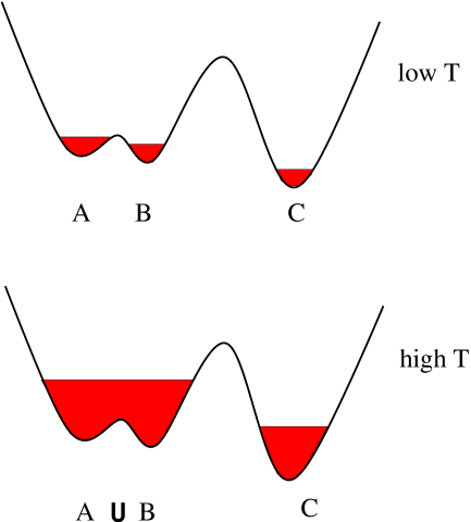
Figure 1: Sketch of temperature dependence of the partitioning in metastable states in a three-well potential model. At low temperature the saddle separating the minima A and B is sufficiently high to provide a separation of time scales. When thermal agitation increase, the explored regions around the minima of the energy landscape (shaded areas) become wider.

In order to determine the NMS at a given non-zero temperature we employ the recursive renormalization procedure proposed in grafi2D . Its main ingredient is the single coalescence step illustrated in Fig. 2: if one of the energy barriers separating node 1 from node 2, $W_{12}$ or $W_{21}$, is smaller than the current temperature, the two nodes coalesce together forming a new node $A$. Between the possible paths from and to the new node, those with minimal energy barrier are kinetically the more relevant. We chose therefore to consider $A$ as connected to the rest of the NMS only by means of the minimal energy connections. For example, considering node 3 in Fig. 2, the relevant connection would be $W_{A3}=$min$(W_{13},W_{23})$ and $W_{3A}=$min$(W_{31},W_{32})$.

The actual implementation of the algorithm is as follows. First of all, we sort all connections in ascending order according to their energy barrier. Then, starting from the first connection, we apply the following iterative procedure to all connections whose energy barrier is lower than the reference temperature:

• The minimal energy node connected by the selected saddle is identified and its label replaces the label corresponding to the other node interested by the connection in the entire connections database.

• The database of connections is searched for eventual multiple connections between the same pairs of nodes. When such connections are found only the one characterized by the lowest energy barrier is kept and the other ones are erased.

• The selected connection is finally erased from the database.

This renormalization algorithm allows to determine the NMS at any given temperature starting from the zero-temperature NMS. As already stressed, the surviving nodes do not represent minima anymore but collections of minima that are best interpreted as metastable states.

We notice that in general the renormalization process tends to increase the average connectivity of the NMS since the new node emerging from the coalescence of two neighboring nodes inherits all their connections. This effect, however is partially mitigated by the presence of shared connections between the coalescing nodes. Defining the average connectivity $c$ as the average number of links per node and calling $k$ the number of shared connections between two coalescing nodes, it can be easily shown that $c$ will decrease upon renormalization only if $k>c-2$.

The large scale dynamics of the original molecular model is now suitably described by a diffusion on the NMS. This process is governed by a linear master equation

$$\frac{{d}P_{i}(t)}{dt}=-WP_{i}(t)$$ (6)

where $P_{i}(t)$ is the probability of residing on the $i$-th node of the graph at time $t$, while $W$ is a temperature dependent Laplacian matrix whose elements are determined by the rates of transition between different nodes,

$$W_{ij}=\delta_{i,j}\sum_{k=1}^{N}\Gamma_{jk}-\Gamma_{ji}\,\,\,$$ (7)

with $\Gamma_{jk}$ being the probability per unit time of a transition from node $j$ to node $k$.

If the NMS is globally connected, the Laplacian matrix has only one eigenvector with zero eigenvalue corresponding to the stationary probability distribution on the graph. Moreover, it can be shown that the Laplacian matrix of the zero-temperature NMS is semi-positive-definite, and direct computation show that this feature is conserved by the renormalization procedure grafi2D . As a consequence, Eq. (6) describes the relaxation to equilibrium on the graph.

By dropping the kinetic information $\Gamma_{jk}$ one can define a discrete Laplacian matrix $\bar{W}$ given by

$$\bar{W}_{ij}=\left\{\begin{array}[]{lccr}1&&\text{if ~{}}{\Gamma}_{ij}\not=0\\ 0&&\text{if ~{}}{\Gamma}_{ij}=0\end{array}\right.$$ (8)

that can be interpreted as describing the process of relaxation to equilibrium in a time unit corresponding to the number of jumps between different nodes. We will see later that the spectral properties of the discrete Laplacian matrix provide useful insights on the topological properties of the NMS.

Figure 2: Coalescence of two nodes. If one of the energy barriers separating 1 from 2, $W_{12}$ or $W_{21}$, is smaller than the reference temperature, the two nodes coalesce together forming a new node $A$ that is connected to node 3 by a single energy barrier, which is min$(W_{13},W_{23})$ to go from $A$ to 3, and min$(W_{31},W_{32})$ to come back from 3 to $A$.

V Thermodynamics

In order to assign a clear quantitative meaning to the temperature scale in our model we determine the folding transition and the $\Theta$-transition temperatures of each sequence. The use of the term “transition” in this context must be clarified. The systems we study are far from the thermodynamic limit, so that no sharp thermodynamic transition occurs and a transition temperature is not rigorously defined. Nonetheless, a change in the thermodynamic behavior does occur in a relatively narrow temperature range, so that it is customary to refer to a “$\Theta$-transition temperature” and a “folding temperature” even for short polymers. When the transitional phenomenon under investigation has a sharp counterpart in the thermodynamic limit (as is the case with the $\Theta$-transition) the finite-size transition temperature is determined using methods which would give the correct result in the thermodynamic limit. The case of the folding transition is different because it does not have a thermodynamic limit counterpart dill2 ; cecco , and various methods have been proposed to give a definition of a folding temperature, which typically yield comparable results tlp .

For convenience we measure the temperature in multiples of $k_{B}$, which is then formally set as $k_{B}=1$. The folding transition was primarily determined by using the “50% criterion”: the system at its folding temperature has equal probability of residing in the native structure as outside of it. As far as the $\Theta$-transition temperature is concerned, one should in principle be able to easily determine it by the presence of maxima of either the specific heat $C_{v}$ or of the derivative of the gyration radius with temperature, $R^{\prime}=\partial_{T}R$. An estimate of these quantities can be easily computed by expanding the potential energy at the second order in the fixed points. The partition function of the system can then be expressed as a sum over all minima:

$$Z(\beta)=\sum_{i}{e^{-\beta V_{i}}\over\Omega_{i}}$$ (9)

where $V_{i}$ is the potential energy of minimum $i$ and $\Omega_{i}$ is the product of non-zero eigenfrequencies of the relative Hessian ${\mathcal{H}}_{i}$. If we translate this in a local entropy $S_{i}=-k_{B}\ln\Omega_{i}$, the probability of residing in the $i$-th minimum can be written as a function of the local free energy $V_{i}-TS_{i}$,

$$p_{i}(\beta)=\frac{1}{Z(\beta)}{e^{-\beta(V_{i}-TS_{i})}}$$ (10)

For a given configuration-dependent quantity $\Xi$, the average value on the landscape can then be expressed as

$$\langle\Xi(\beta)\rangle=\sum_{i}\Xi_{i}p_{i}(\beta).$$ (11)

In this contest quantities such as the specific heat $C_{v}=\partial\langle E\rangle/\partial T$ and the average gyration radius (mean square distance of the chain elements form their center of mass) can be computed once the configurations corresponding to each minimum are known. The quality of this approximation has been thoroughly tested for several rough energy landscapes parisi ; wales showing, as far as protein models are concerned, a reasonable accuracy at temperatures comparable with the folding and $\Theta$-transitions mc .

Clearly the definition of the folding transition based on the 50% criterion suffers of eventual ambiguities in the determination of the native configuration. The homopolymers that we model tend to be affected by this problem. Due to the fact that the energy of homopolymers is invariant upon chain-reversal, the minima of the potential have a symmetric image, excluding those for which the two symmetric images coincide. We find that the probability that the absolute minimum has a non-symmetric configuration are very high and in the sequences analyzed only the hydrophobic homopolymer of length $N=10$ does not fall in this category. In all other cases energy has two symmetric global minima, and they must both be used in order to correctly implement the 50% criterion described above. Analogously, due to the finite size of the systems under study, also the determination of the $\Theta$-transition temperature might be strongly affected by the parameter used to define it tlp . In this model the two consensus choices, $C_{v}$ and $R^{\prime}$, give very similar indications. More precisely, for each sequence analyzed, the specific heat shows two maxima, and the lower one in temperature always coincides with $T_{f}$ as determined by means of the 50% criterion. $R^{\prime}$ might instead show either two maxima, or a pronounced minimum and a maximum, the minimum always appearing at lower temperature than the maximum. The high temperature maximum almost coincide with the second maximum of the specific heat, thus reinforcing the interpretation of the latter as a sign of the $\Theta$-transition. Also the first minimum/maximum always occurs at the same temperature as the first peak of the specific heat, which, as we already noted, corresponds to $T_{f}$. Fig. 3 shows this agreement between $C_{v}$ and $R^{\prime}$ for the hydrophobic homopolymer of length 12, while Fig. 4 shows an example of negative $R^{\prime}$ peak at $T_{f}$ occurring for the unstructured heteropolymer.

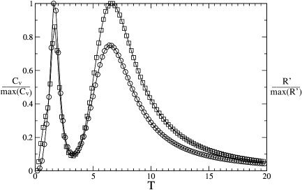
Figure 3: Specific heat (circles) and derivative of the gyration radius (squares) as a function of temperature for the hydrophobic homopolymer of length 12. To ease comparison both quantities are normalized to their maximum value.

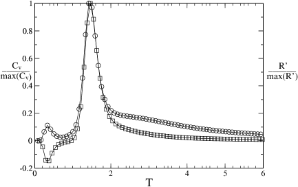
Figure 4: Specific heat (circles) and derivative of the gyration radius (squares) as a function of temperature for the unstable heteropolymer. To ease comparison both quantities are normalized to their maximum value.

An inspection of the gyration radii of individual minima shows that a negative $R^{\prime}$ peak appears when the native minimum does not have the minimal gyration radius. As a consequence, the gyration radius might decrease as soon as the system starts exploring other configurations, eventually increasing again when higher temperatures force it towards swollen conformations. In both cases the presence of either a minimum or a maximum in $R^{\prime}$ amounts to a change in convexity of the $R$ versus temperature and, once again, signals that the system is undergoing a significant change in its configurational trends.

The $\alpha$-helix-like heteropolymer shows instead only one peak in the specific heat. This thermodynamic behavior is akin to what observed in similar systems lapo , where no molten globule state could be detected. In those cases $T_{\Theta}$ and $T_{f}$ coincide. Therefore, this sequence is structurally very stable, its native configuration being dominant even at temperatures almost as high as the temperature of thermal unfolding. Also in this case the derivative of the gyration radius shows a minimum corresponding to the folding transition, since the native state is an elongated helical structure while other minima have a smaller gyration radius.

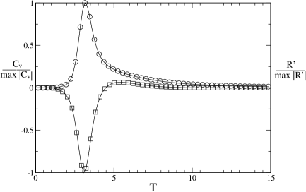
Figure 5: Specific heat (circles) and derivative of the gyration radius (squares) as a function of temperature for the stable heteropolymer. To ease comparison both quantities are normalized to maximum of their absolute value.

In order to illustrate the agreement between the different criteria for the determination of $T_{f}$ in table 1 we report the folding temperature as computed by means of the 50% criterion and relying on the first maximum of the specific heat. $T_{\Theta}$ is also reported.

	$T_{f,0}$ (n)	$T_{f,1}$	$T_{\Theta}$
Stable12	3.95 (1)	4.2	4.2
Unstable12	0.21 (1)	0.33	1.5
Homo12	1.25 (2)	1.6	6.5
Homo11	1.1 (2)	1.4	4.2
Homo10	0.6 (1)	0.6	3.1
Homo09	1.3 (2)	2.0	2.5
Homo08	1.0 (2)	1.0	0.9

Table 1: Folding and $\Theta$-transition temperatures for the sequences under study. Folding temperatures are determined by means of the 50% criterion ($T_{f,0}$) and relying on the first peak of the specific heat ($T_{f,1}$). Near $T_{f,0}$ we report in brackets the number $n$ of minima used to determine it.

It is interesting to notice that the ratio between $T_{f}$ and $T_{\Theta}$, which might be considered as a relative measure of the stability of their native structure, is approximately the same (4$\div$5) for the homopolymer of length 12 and the unstable folder.

This table also reveals an interesting feature of the thermodynamics of homopolymers and its dependence on the system size: while $T_{\Theta}$ grows with the polymer length (hydrophobic compaction is modelled by two-body interactions whose effect grows with the chain length), $T_{f}$ does not show any well defined trend and oscillates around a fixed value $\bar{T}_{f}$. The value of the temperature $\bar{T}_{f}\simeq 1.1$ determined by using probabilities is slightly lower than the value $\bar{T}_{f}\simeq 1.4$ determined by using the specific heat.

In order to show that the energy landscape of homopolymers of different length has basically the same shape apart from a scaling factor $N^{2}$, in Fig. 6 we report the histogram $\rho(\bar{V}_{m})$ of the rescaled potential $\bar{V}=VN^{-2}$ in each minimum. The histograms of the homopolymers of lengths $N=10,11,12$ collapse onto the same curve. It must however be stressed that, since the Lennard-Jones potential is short-range, the number of units that can possibly interact with a given monomer is limited. As a consequence, for large systems we expect the energy to scale linearly with the chain length $N$. The almost perfect $\sim N^{2}$ scaling observed signals therefore that the systems studied are still very small, their linear dimension being comparable to the Lennard-Jones range.

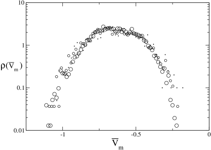
Figure 6: Histogram of the rescaled potential $\bar{V}$ of the minima of the potential energy for the homopolymers of lengths $N=10,11,12$. The rescaling factor is $N^{-2}$. The circles radius is proportional to $N$.

In order to clarify the other observed trend, the independence of $T_{f}$ on systems size, we preliminary observe that increasing the system size leads to a fast increase of the landscape roughness especially if measured in terms of number of minima and saddles. Figure 7 shows that, as expected in these systems, $N_{\mathrm{min}}$ grows exponentially with the chain length $N$. The same holds for the number of saddles $N_{\mathrm{sad}}$ but with a different algebraic correction. Indeed, the ratio between these two quantities, which corresponds to half the average connectivity of the NMS, grows linearly with $N$ (see inset in Fig. 7).

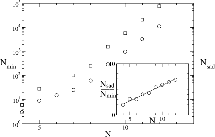
Figure 7: Number of minima $N_{\mathrm{min}}$ (circles) and saddles $N_{\mathrm{sad}}$ (squares) for increasing chain length $N$. In the inset the ratio $N_{\mathrm{sad}}/N_{\mathrm{min}}$ is reported together with a power law fit (exponent 1.07).

It must now be noted that not only the number of minima increases with system size but also the total volume of the available configurational space does so. It is thus reasonable to expect that their ratio, the average volume of the basin of attraction of each minimum, will also experience an exponential dependence from $N$. The logarithm of the volume of an attraction basin corresponds to its entropy. As already mentioned, this can be estimated according to a second order approximation in the local energy minimum:

$$S=-k_{B}\sum_{k}^{3N-6}\log(\omega_{i}^{(k)})$$ (12)

where the $\omega_{i}^{(k)}$’s are the $3N-6$ non-zero eigenfrequencies — i.e., square root of the eigenvalues — of the Hessian matrix in the minimum $i$. In Fig. 8 we report the histograms of the entropies for homopolymers of various length after rescaling by a factor $N^{-1.15}$. The rescaling factor was chosen in order to force the collapse of all histograms onto a single curve and witnesses an approximately linear dependence of the average basin entropy on chain length.

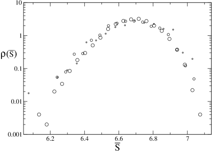
Figure 8: Histogram of the rescaled entropy $\bar{S}=S/N^{1.15}$ of the minima of the potential energy for the homopolymers of lengths $N=10,11,12$. The symbol size is proportional to $N$.

As far as the stability of the folding temperature is concerned, we recall that $T_{f}$ indicates the point where the free energy of the native configuration is approached also by other minima. An increase of the system size would therefore produce two counteracting effects on $T_{f}$. On the one hand the average steepness of the landscape will increase, thus increasing the energetic gap between the native configuration and its neighbors, on the other hand the total number of minima will also quickly increase, compacting minima in the configuration space and consequently in energy.

Finally we note that the distribution $\rho(V_{s})$ of the first-order saddles energies $V_{s}$ shows a dependency on system size very similar to that of the energy of the minima (data not shown). It is therefore tempting to picture the effect of increasing chain lengths as a simple isometric stretching of the energy landscape, as could be attained by multiplying energy by a constant factor. This picture apparently clashes with the observation that the profiles of the histograms of the energy barrier heights $W$ are pretty similar for all chain lengths, and consistent with the same exponential function (see Fig. 9).

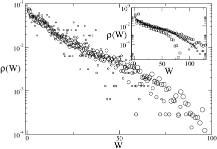
Figure 9: Histogram of energy barriers $W$ between connected minima for homopolymers with $N=10,11,12$. The symbol size increases with $N$. Inset: distribution of energy barriers for the unstable folder (squares), stable folder (circles) and homopolymers with $N=12$ (crosses).

Also this effect, however, can be accounted for by the quick growth of competing minima. The appearance of new minima helps breaking conformational transitions in more sub-steps, thus counteracting the general quadratic increase of their energetic cost.

VI The hydrophobic homopolymers: topology as a function of temperature and system size

The thermodynamic properties analyzed so far only depend on the distribution of the minima of the potential energy. In order to account for the trends observed in the folding and $\Theta$-transition temperature we were led to analyze in some detail the chain length dependence of the energy landscape both in terms of minima and connection saddles. Since potential energy minima correspond to nodes of the zero-temperature NMS and saddles correspond to its links, the results of the previous analysis might be rephrased in terms of an exponential growth of the graph degree with system size and a linear growth of its average connectivity. We will now extend this analysis to the finite-temperature NMS. More precisely we will focus on the combined effects of temperature and systems size on the topology of the NMS for homopolymers.

The first quantity affected by the renormalization process is obviously the graph size. The total number of nodes for each homopolymer is reported in Table 2 for various temperatures corresponding to fixed multiples of $\bar{T}_{f}$ (the average folding temperature for homopolymers, determined using the peak in the specific heat) namely $0.5\bar{T}_{f}$, $\bar{T}_{f}$ and $1.5\bar{T}_{f}$. Graph sizes appear to decay exponentially with temperature, with a decay rate growing approximately linearly with the chain length.

$N$	$T=0.0$	$T=0.7$	$T=1.4$	$T=2.1$
12	11120	5276	2684	1372
11	3313	1754	976	532
10	999	564	356	228
09	300	197	159	106
08	104	67	51	36

Table 2: Graph size during renormalization at four different temperatures, for homopolymers of different lengths.

A similar, yet more irregular, decay can be observed in the number of links of the renormalized graph reported in table 3.

$N$	$T=0.0$	$T=0.7$	$T=1.4$	$T=2.1$
12	73468	50802	17374	5700
11	20392	14974	7752	2456
10	5710	4236	2920	1600
9	1562	1280	1130	794
8	482	364	298	210

Table 3: Total number of connections during renormalization at four different temperatures for five hydrophobic homopolymers of different lengths.

In order to understand whether the process of node coalescence that causes the NMS to shrink with temperature proceeds uniformly on the NMS, we analyze the temperature dependence of the multiplicities $m_{i}$ of each node, i.e., the number of nodes of the zero-temperature graph that coalesced into the $i$-th node. In Fig. 10 we report the histograms of $m_{i}$ for the $N=12$ homopolymer at various temperatures. The isolated column developing on the right of the figure represents the multiplicity of the minimal energy node that is growing at the expense of the nodes with intermediate multiplicity ($m_{i}>10$). The low multiplicity nodes are almost unaffected. These observations suggest that low saddles are highly localized around the bottom of the energy landscape. Concerning the latter point, we recall that two nodes coalesce when they are separated by a link corresponding to a saddle of energy lower than the current temperature. If the majority of nodes tend to coalesce on the minimal energy node, it means that this node is, at every temperature, the one characterized by the lowest energy connections. Furthermore, the fact that isolated nodes of intermediate multiplicity, i.e., isolated regions of the landscape characterized by the presence of low energy saddles, end up very early in the minimal energy node reinforces the above picture on the localization of low energy saddles.

The presence of a unique metastable state around and above $T_{f}$ implies that, at these temperatures, long homopolymers are characterized by the presence of an extended, fast-connected, low-energy region where local rearrangements take place more quickly than in the rest of the landscape.

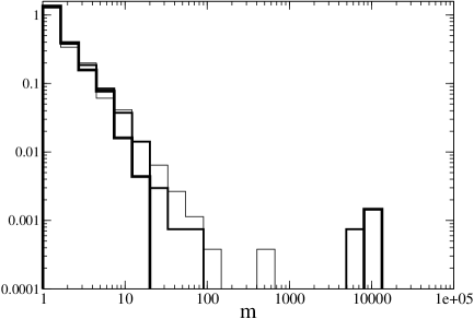
Figure 10: Histograms of the multiplicities $m_{i}$ of each node of the renormalized graph for the $N=12$ homopolymer at temperatures $T=0.7,1.4,2.1$. Increasing temperatures are represented by lines of increasing thickness.

The opposite scenario emerges when looking at shorter chains where the fraction of low multiplicity nodes decreases. For example in Table 4 we report, for the various homopolymers, the fraction of nodes with multiplicity 1 at different temperatures. This is the fraction of nodes still untouched by renormalization and, therefore, separated from the rest of the NMS by steep activation barriers. Table 4 shows that short homopolymers are more affected by renormalization and loose most of their nodes of multiplicity 1.

$N$	$T=0.7$	$T=1.4$	$T=2.1$
12	0.67	0.65	0.67
11	0.67	0.63	0.65
10	0.70	0.62	0.59
9	0.70	0.65	0.61
8	0.65	0.52	0.41

Table 4: Fraction of the nodes of the renormalized NMS having multiplicity equal to one. Data refer to hydrophobic homopolymers of different lengths at various temperatures.

This phenomenon might be due to two slightly different mechanisms: either the low energy node directly attracts low multiplicity nodes or the renormalization process affects in the same manner nodes of all multiplicities. In both cases the previous argument about the spatial localization of low energy barriers near the native minimum falls and the landscape can no longer be divided in slow and fast regions. Remarkably, the difference in the spatial distribution of energy barriers on the landscape described above arises independently from the actual probability distribution of barrier heights $\rho(V_{s})$ (see Fig. 9) which, we recall, is pretty much size-independent.

Finally, to document the relative importance of the fast-connected central regions in the different sequences analyzed, we report in Table 5 the number of minima of the potential attracted by the maximally growing node in the graph. This almost always coincides with the minimal energy node except for four low temperature cases dubbed with a star in the table. A comparison at the same temperature between homopolymers of different lengths shows that the fraction of minima attracted by the minimal energy node (in parenthesis in the table) grows with the chain length.

$N$	$T=0.7$	$T=1.4$	$T=2.1$
12	453 (0.04)	5908 (0.53)	8828 (0.79)
11	52 (0.02) *	1043 (0.31)	2324 (0.70)
10	38 (0.04) *	117 (0.18)	429 (0.43)
9	6 (0.03) *	18 (0.06)	57 (0.19)
8	4 (0.04) *	7 (0.06)	21 (0.20)

Table 5: Multiplicity of the maximally growing node during renormalization at three different temperatures for homopolymers of different lengths. When the maximally growing node does not correspond to the minimal energy node data are labeled with a star. The fraction of minima coalesced to the minimal energy node is reported within parentheses.

It can be observed that by adding the number of nodes at a given temperature (Table 2) to the number of minima coalesced to the minimal energy node one gets a much higher proportion of the total number of minima for long chains than for short ones. For example, at $T=2.1$ the $N=12$ polymer has $8828$ minima in the minimal energy node and $1372$ nodes surviving on the graph. The latter nodes were much less affected by the merging process, with only about a decrease of about 10% of their number. In the $N=10$ case the decrease is instead of 35%, once again implying that coalescence is more uniformly distributed in this graph.

In the previous section we documented the linear increase of the average connectivity of the graph with the system size. At finite temperatures this quantity displays a more complex behavior, as shown in Table 6 where the average connectivity $c$ of the renormalized graphs of the five homopolymers is reported. After an initial growth the longer chains show a decrease of the average connectivity with temperature while the two shorter ones exhibit a growing connectivity up to $T=2.1$. The temperature of peak connectivity diminishes with the chain length.

$N$	$T=0$	$T=0.7$	$T=1.4$	$T=2.1$
12	13.2	19.3	12.9	8.4
11	12.2	17.0	15.9	9.2
10	11.4	15.0	16.4	14.0
9	10.4	13.0	14.2	15.0
8	9.2	10.8	11.6	12.0

Table 6: The average connectivity $c$ for five hydrophobic homopolymers of different lengths at various temperatures.

Figure 11 shows the effect of temperature on the distribution of the connectivities $n_{i}$ for the homopolymer of chain length 12 and 10 (inset).

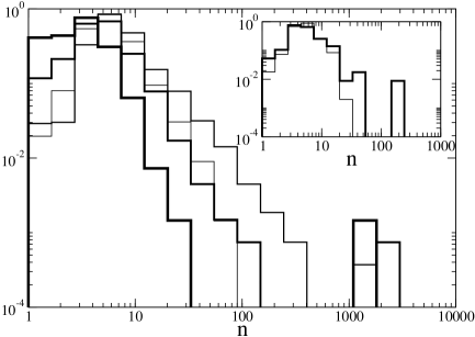
Figure 11: Histograms of the number $n_{i}$ of contacts of each node for the $N=12$ and $N=10$ (inset) homopolymers at temperatures $T=0.0,0.7,1.4,2.1$ and $T=0.0,2.1$ respectively. Increasing temperatures are represented by lines of increasing thickness.

While the total number of connections is almost invariant upon renormalization for the shorter systems, the longer one shows a remarkable loss of connectivity above $n_{i}=10$. In both cases the growth of an isolated, high connectivity region is observed. A closer inspection reveals that this region corresponds to the minimal energy node that, while attracting its neighbors, gradually acquires new connections. It is thus tempting to ascribe the observed differences in average connectivity to the different rates of coalescence to this node previously observed in long and short chains. We remind that the average connectivity $c$ decreases upon renormalization only if there are many shared connections between the coalescing nodes. The average connectivity increases significantly during the fast initial growth of the “central” node, signaling that each coalescing node is bringing new connections. As a consequence the ramifications of the “central” node are expanding in areas of the NMS which were previously relatively remote in terms of connections. After that phase a decrease in connectivity begins, showing that any new node attracted by the fastest growing node brings only a few new connections: the central Node has now a direct link to almost every portion of the NMS.

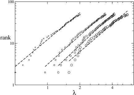
Figure 12: Rank-to-eigenvalue plot for the Laplacian matrix of the hydrophobic homopolymer of length 9 at increasing temperature: $T=0.0$, $0.7$, $1.4$, $2.1$. The circles radius is proportional to temperature. Dashed lines represent least-square power-law fits to the data.

We now describe the spectral properties of the NMSs of the sequence studied. More specifically we investigate their spectral dimension because it determines the large scale diffusivity on the graph. The spectral dimension describes the spectral density of the discrete Laplacian matrix for small eigenvalues. Since small eigenvalues correspond to long relaxation paths, high spectral dimensions imply a relaxation to equilibrium that requires a long series of jumps between nodes. Hence, although lacking any direct kinetic information, the spectral dimension provides information about the dynamics of the system. In Fig. 12 we illustrate the numerical procedure for the determination of the spectral dimension for the $N=9$ homopolymer at various temperatures. After a numerical diagonalization of the Laplacian matrix of the NMS the resulting eigenvalues are rank ordered. The resulting rank-to-eigenvalue curve is proportional to the integrated spectral density and can be fitted with a power law in order to extract the spectral dimension $\bar{d}$. It must be stressed that one can rigorously assign a topological meaning to $\bar{d}$ only for asymptotically large graphs: several invariant properties of the spectral dimension, such as invariance under local link rewiring, only hold in the limit of infinite size. One might thus try to estimate the effects of the finite size of the analyzed graphs by quantifying the amount of such non-invariance. Before evaluating $\bar{d}$ we therefore altered each NMS by adding random links between second neighbors (non-directly connected nodes connected to each other by a third node). The procedure was repeated 50 times generating 50 different realizations of each NMS and 50 different estimates of $\bar{d}$ (see Fig. 13 where a sample of the rank-to-eigenvalue plots obtained after random rewirings is reported). Since this quantity should be invariant by link addition the standard deviation of the values obtained with this procedure provides a measure of the numerical error in its estimate. The resulting averages $\langle\bar{d}\rangle$ are reported in Table 7. The associated statistical errors range from 3% to 5%.

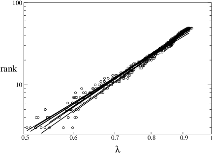
Figure 13: Rank-to-eigenvalue plot for the Laplacian matrix of the hydrophobic homopolymer of length 12 for different random rewirings.

The spectral dimension grows for the homopolymers more quickly than the dimension of the associated configurational space. On the other hand, at least for short polymers, it does not appreciably change with temperature coherently with the expected isospectrality of the renormalization procedure.

$N$	$T=0.0$	$T=0.7$	$T=1.4$	$T=2.1$
12	16.4	16.4	8*	5.6*
11	8.8	12.4*	*	*
10	6.4	6.0	5.6	*
9	4.2	4.6	4.8	4.4
8	3.2	3.0	2.8	2.8

Table 7: Average spectral dimensions of the five homopolymers for different chain lengths at different temperatures. Data marked with a star refer to spectra with a significant number of $\lambda$=1 eigenvalues. Missing data refer to cases where not enough points where available below $\lambda$=1 to allow a reliable fitting.

For longer polymers the spectral dimension estimate $\bar{d}$ is affected by an unexpected spectral feature: at a certain temperature the Laplacian spectral density peaks around $\lambda=1$. It can be shown that these eigenvalues are due to nodes connected to more than one leaf node (by leaf we mean a node with only one link). Initially the presence of a node connected to two or more leafs is rare but, as renormalization goes on, it tends to increase. The appearance of $\lambda=1$ eigenvalues is therefore enhanced by a high coalescence rates. As shown above, long homopolymers are indeed characterized by the fast coalescing region of the lowest-energy minimum, which explains the early appearance of the mark of multiple leaf nodes in their spectra. This phenomenon is depicted in Fig. 14 where the rank-to-eigenvalue plot for the $N=12$ at various temperature is reported. Ranked data have been multiplied by an arbitrary factor to ease reading. At low temperatures the curves are pretty much invariant and spectral density is conserved. At $T=1.4$, however, a step appears in the curve at $\lambda=1$ (corresponding to a Dirac $\delta$ peak in the spectral density coming from the abundance of leaf nodes). Notably a steep drop in the spectral dimension can be observed at the same time and persist at higher temperatures while the step at $\lambda=1$ grows.

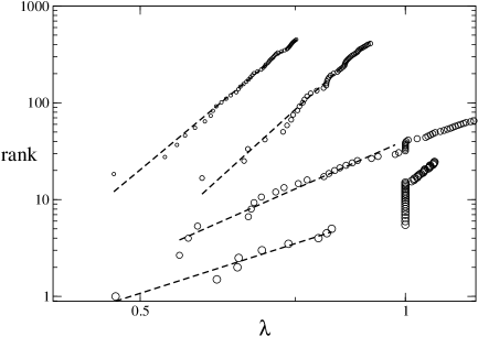
Figure 14: Rank-to-eigenvalue plot for the Laplacian matrix of the hydrophobic homopolymer of length 12 at increasing temperature: T=0.0, 0.7, 1.4, 2.1. Larger symbols correspond to higher temperature. Rank data were multiplied for an arbitrary factor to ease reading. Dashed lines represent least-square power-law fits to the scale invariant portion of the curves.

Table 7, however, shows that, although the appearance of leaf nodes — labeled by stars in the table — is often associated with changes in the spectral dimension, the latter do not share a clearly defined direction. In some cases ($N=11$) $\bar{d}$ increases after the appearance of $\lambda=1$ eigenvalues while in others ($N=12$) it decreases. Moreover, in a few other cases the spectral dimension could not be estimated because not enough data where available below $\lambda$=1 (to allow a reliable fit), and fitting above this value does not seem correct since rank-to-eigenvalue curves appear either to quickly lose any scale-invariant character for $\lambda=1$ or to display a markedly different exponent (see the $T=2.1$ curve in fig 14). Such anomalies therefore suggest that the procedure here highlighted for the computation of the spectral dimension looses meaning in presence of pronounced peaks in the spectral density.

VII The heteropolymers: topology as a function of sequence

The effect of the primary sequences on the topological properties of the NMS is now determined by investigating the two heteropolymers with 12 residues and by comparing the results with those for to the $N=12$ homopolymer.

A first fundamental difference between the stable heteropolymer and the other sequences arises already at $T=0$ when considering the size of the NMS, which at this temperature simply corresponds to the number of minima of the potential energy. The strong energetic bias and the relative lack of frustration of this system result in a much smaller quantity of minima, 4128, than in the case of the weakly biased unstable heteropolymer which has instead 13394 minima. The latter is much more similar to the homopolymer which, we recall, has 11120 minima. The lower number of possible kinetic traps to be overcome by the stable heteropolymer already suggests its higher folding propensity. On the contrary the picture provided by considering NMS connectivities is much less clear, since the average number of connecting saddles for each minimum is $16.0$ for the stable heteropolymer and $27.4$ for the unstable one while it was $13.2$ for the homopolymer of equal length. No particular correlation with structural stability can be therefore observed.

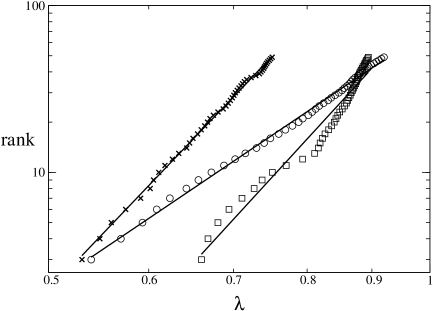
Figure 15: Rank-to-eigenvalue plot for the Laplacian matrix of unstable folder (squares), stable folder (circles) and homopolymer with $N=12$ at $T=0$. Continuous lines represent least-square power-law fits to the data.

This scenario is further emphasized by a topological difference between the zero-temperature NMS of the stable heteropolymer and the other sequences. While the spectral dimension of the unstable heteropolymer is comparable to that of the homopolymer of equal length ($\bar{d}=16.6\pm 0.9$ in the first case and $\bar{d}=16.4\pm 0.9$ in the latter), the stable folder is characterized by a much smaller spectral dimension: $\bar{d}=10.3\pm 0.6$. These differences are preserved also at higher temperatures since, also in this case, spectral dimensions keep substantially unchanged until the appearance of $\lambda=1$ eigenvalues. We recall that the unstable heteropolymer and the $N=12$ homopolymer also share a very similar ratio $T_{f}/T_{\Theta}$. The spectral dimension, a topological quantity that describes relaxation dynamics, does therefore correlate with the latter ratio, which is a thermodynamical quantity.

This finding relates with analogous evidence grafi2D for a two-dimensional toy model where a difference in the spectral dimension between heteropolymers and homopolymers was detected. In that case, however, the spectral dimension was not found to depend on the stability of the native structure but rather on the amount of heterogeneity in the sequence. Different sequences displaying different folding behaviors and landscape steepness but the same ratio of polar to hydrophobic beads shared the same spectral dimension. Moreover, such a dependency only appeared in that model for finite-temperature NMSs, while here it is evident already at $T=0$.

The two heteropolymers analyzed here share the same fast decay of the tails of the energy barriers distribution seen for the homopolymer (see inset in Fig. 9). In the heteropolymer case the decay is slightly faster and leads to a substantial cutoff at $V_{s}\simeq 80$ for the unstable folder. A far more fundamental difference, however, arises at small energies. The unstable folder differs from the two other sequences in having a much higher fraction of low barriers, $V_{s}<10$. Since this is the region most affected by the renormalization procedure, it is reasonable to expect a different behavior of this sequence under renormalization. Indeed, the comparison of the topological changes induced by the renormalization process on the NMSs of polymers characterized by different primary sequences proves very instructive about the origin of the above mentioned leaf node phenomenon. It is not obvious which physical meaning to assign to the gradual transformation of the NMS in a stellar graph characterized by a center surrounded by leaf nodes. It is also equally non-intuitive what relation might this process have with the thermodynamics of the system. The analysis of the spectra of the sequences analyzed (see Table 8) shows that $\lambda=1$ eigenvalues always become dominant at $T_{\Theta}$ implying that at that temperature leaf nodes become the only relevant feature of the NMS. In fact, at $T_{\Theta}$ the graph has already shrunk in size by more than one order of magnitude and almost all of the missing nodes appear to have merged to the minimal energy node, which seems thus to be the hot-spot of renormalization also for heteropolymers.

Analyzing the same indicators at lower temperatures (columns referring to $T=\frac{2T_{\Theta}}{3}$ in Table 8) shows, however, a marked difference in the progress of the appearance of leaf nodes against other topological transformations of the NMS. While at $T=\frac{2T_{\Theta}}{3}$ the minimal energy node has eaten up already all the available configuration space, still the relative amount of $\lambda=1$ is significantly smaller than the value it takes at $T_{\Theta}$. The appearance of leaf nodes seems therefore to be intimately connected with the $\Theta$-transition in these sequences, depicting the moment in which all the configuration space becomes equally accessible. In this condition the metastable states still persisting as separate nodes are very unlikely to have multiple connections because all of their neighbors already collapsed on the minimal energy node. As a consequence these nodes, which originally corresponded to the frontier of the low temperature NMS, have a large probability of becoming a leaf node shortly before coalescing themselves to the minimal energy node.

The pace of this process is strongly sequence-dependent and does not show any clear correlation with the stability of the native structure. It nonetheless appears to start at markedly low temperatures for homopolymers.

	surviving		multiplicity of		eigenvalues
	nodes		largest node		with $\lambda=1$
	$T=\frac{2T_{\Theta}}{3}$	$T=T_{\Theta}$	$T=\frac{2T_{\Theta}}{3}$	$T=T_{\Theta}$	$T=\frac{2T_{\Theta}}{3}$	$T=T_{\Theta}$
Stable12	155	73	0.94	0.97	0.52	0.74
Unstable12	402	170	0.96	0.99	0.37	0.91
Homo12	109	54	0.99	0.99	0.88	0.93

Table 8: Number of surviving nodes, fraction of nodes in the minimal energy node and fraction of eigenvalues $\lambda=1$ for the three polymers of length 12 during renormalization.

Furthermore, we remember that the the appearance of leaf nodes also depends on chain length. Shorter polymers have a less marked frequency of $\lambda=1$ eigenvalues also in the proximity of $T_{\Theta}$ (Table 7). It is therefore worth stressing the differences in the $\Theta$-transition in short and long polymers. Regardless of chain length, the $\Theta$-transition signals the temperature at which all configuration space becomes equally accessible. When this happens in short polymers, the landscape is still divided into different metastable states or, equivalently, there are still kinetic barriers to be overcome to access the whole configuration space. On the contrary, in long polymers, at the $\Theta$-transition almost all the configuration space belongs to the same stationary state and can be quickly sampled without crossing kinetically relevant barriers. This does not mean that large barriers are absent from the energy landscape, on the contrary they are as common as in short polymers. Their arrangement, however, is not capable of dividing the landscape into kinetically separate metastable states.

VIII Conclusions

We analyzed the thermodynamics as well as some metric and topological properties of the NMS of short homopolymers and heteropolymers in a coarse-grained off-lattice protein model. The homopolymers were hydrophobic in nature and characterized by different lengths, while the two heteropolymers were chosen in order to ensure a marked difference in structural stability.

The systems investigated exhibit a variety of thermodynamical behaviors with respect to folding. While some sequences show all three classical protein conformational arrangements –including the molten globule– others pass directly from folded to swollen, thus reproducing the tendency of stable folders to have high $T_{f}$. The model considered is therefore able of efficiently mimicking the differences of folding propensities observed in real protein sequences.

We have employed a recently proposed procedure grafi2D to generate the NMS at a finite temperature $T$, based on the merging of nodes separated by energy barriers lower than $T$. This renormalization procedure allows to determine a partition of the configuration space into dynamically separated regions. We have thus studied the temperature dependence of the NMS characteristic of each sequence. The analysis of the topological properties of the NMS of homopolymers of different lengths highlights how the statistical distribution of activation energies is not the only factor determining the behavior of the graph under renormalization: the spatial distribution of the barriers also plays a crucial role. Indeed, although investigated homopolymers share the same distribution of energy barriers, their topology respond pretty differently to an increase in temperature. While in long sequences the renormalization procedure mainly alters the low energy region of the landscape where metastable states merge into a unique, rapidly expanding macro-state, in shorter sequences this growth is more uniformly distributed and other, more distant metastable states might experience a substantial expansion. These differences in the renormalization process are reflected in an early (low $T$) tendency to create leaf nodes in the NMS of long sequences, both for homopolymers and heteropolymers. This phenomenon is independent on the stability of the native structures of the sequences analyzed and completes around the $\Theta$-temperature, where the configuration space mostly belongs to same metastable state.

The spectral dimension of the same sequence at different temperatures is approximately constant, at least before leaf nodes appear. Given the same length, the spectral dimension appears to be higher for the sequences characterized by unstable native structures. This finding suggests a non-obvious link between thermodynamics and the dynamical properties of these systems. Sequences characterized by a stable folded state appear to be characterized by shorter and less complicated relaxation paths. Indeed, the stable heteropolymer is characterized by simpler connectivity also in terms of the sheer number of nodes, which, compared to the other $N=12$ sequences, ranges from one half ($T=0$) to one order of magnitude less ($T_{\Theta}$).

Interestingly some of the features described above seem to hold also for a simpler two-dimensional model investigated in grafi2D . Also in that model the spatial distribution of the barriers is crucial in shaping some properties of the energy landscape, namely the amount of kinetic traps. However, in that case only kinetic properties of the NMS were affected and not its topology. On the contrary, in the model here investigated topology is strongly influenced by the spatial distribution of energy barriers. Finally, in both models the spectral dimension helps in categorizing sequences according to the complexity of their relaxation paths. In the two-dimensional model, however, such a difference only arises at finite temperature and is related to sequence frustration rather than to the stability of the native structure.

- (1) P. J. Flory, Principles of Polymer Chemistry, Cornel University Press (Ithaca, NY, 1953).
- (2) C E Soteros and S G Whittington, J. Phys. A: Math. Gen. 37, R279 (2004).
- (3) A. V. Finkelstein, D. N. Ivankov, S. O. Garbuzynskiy, O. V. Galzitskaya, Curr. Protein Pept. Sci. 8, 521 (2007).
- (4) S. A. Hobart, D. W. Meinhold, R. Osuna, W. Colon, Biochem. 41, 13744 (2002).
- (5) A. D. Keefe and J. W. Szostak, Nature 410, 715 (2001).
- (6) K. A. Dill, Biochem. 24, 1501 (1985).
- (7) T. Head-Gordon and S. Brown, Curr. Opin. Struct. Biol. 13, 160 (2003).
- (8) D.J. Wales, Energy Landscapes, Cambridge Univ. Press (Cambridge, 2003).
- (9) L. Angelani, G. Parisi, G. Ruocco, and G. Viliani, Phys. Rev. Lett. 81, 4648 (1998).
- (10) L. Angelani, R. Di Leonardo, G. Ruocco, A. Scala, and F. Sciortino, Phys. Rev. Lett. 85, 5356 (2000).
- (11) V. B. P. Leite, J. N. Onuchic, G. Stelland, and J. Wang, Biophys. J. 87, 3633 (2004).
- (12) J. Wang, Biophys J. 87, 2164 (2004).
- (13) T. Veitshans, D. Klimov, and D. Thirumalai, Folding & Design 2, 1 (1997).
- (14) A. Torcini, R. Livi, and A. Politi, J. Biol. Phys. 27, 181 (2001).
- (15) N. G. Van Kampen, Stochastic processes in physics and chemistry (North Holland, 1981)
- (16) L. Bongini, L. Casetti, R. Livi, A. Politi, A. Torcini, arXiv:0811.3148
- (17) C. Clementi, H. Nymeyer and J. N. Onuchic, J. Mol. Biol. 298, 937 (2000).
- (18) P. Das, S. Matysiak, and C. Clementi, Proc. Nat. Acc. Sci. USA 102, 10141 (2005).
- (19) A. Mossa and C. Clementi, Phys. Rev. E 75, 046707 (2007).
- (20) G. T. Barkema and N. Mousseau, Phys. Rev. Lett. 77, 4358 (1996).
- (21) N. Mousseau and G. T. Barkema, Phys. Rev. E 57, 2419 (1998).
- (22) G Wei, P. Derreumaux, and N. Mousseau, J. Chem. Phys. 119, 6403 (2003).
- (23) N. Mousseau, P. Derreumaux, and G. Gilbert, Phys. Biol. 2, S101 (2005).
- (24) Mi-Ran Yun, R. Lavery, N. Mousseau, K. Zakrzewska, and P. Derreumaux, Proteins: Struct. Funct. Bioinf. 63, 967 (2006).
- (25) http://www.phys.umontreal.ca/~mousseau/
- (26) K. A. Dill, Biochem. 29, 7133 (1990).
- (27) R. Burioni, D. Cassi, F. Cecconi and A. Vulpiani, Proteins: Struct. Funct. Bioinf. 55, 529 (2004).
- (28) L. Bongini, R. Livi, A. Politi, and A. Torcini, Phys. Rev. E 72, 051929 (2005).
- (29) L. N. Mazzoni and L. Casetti, Phys. Rev. Lett. 97, 218104 (2006); Phys. Rev. E 77, 051917 (2008).