Collisionless Magnetic Reconnection in a Five-Moment Two-Fluid Electron-Positron Plasma

Abstract.

We simulate magnetic reconnection in electron-positron (pair) plasma using a collisionless two-fluid model with isotropic pressure. In this model the resistive, Hall, and electrokinetic pressure terms are absent from the curl of Ohm’s law, leaving the inertial term alone to provide for magnetic reconnection. Our simulations suggest that for pair plasma simulated with isotropic pressure fast reconnection does not occur without the aid of sufficient (numerical) diffusion. We contrast this result with simulations and published results showing fast reconnection for collisionless two-fluid plasma with isotropic pressures and non-canceling mass-to-charge ratios, where Hall effects are present and numerical diffusion is small, and with published PIC studies of pair plasma which observe fast reconnection and attribute it to nonisotropic pressure.

1. Introduction

An important issue of controversy in the magnetic reconnection community is the minimal conditions required for fast magnetic reconnection to occur in a plasma and the minimal modeling requirements to resolve it [7]. The first attempt to model reconnection was carried out by Sweet [9] and Parker [6], who used a resistive magnetohydrodynamic (MHD) model. Their approach was only successful in modeling a slow form of reconnection and not the much faster reconnection that is observed in laboratory and space plasma.

The Geospace Environmental Modeling (GEM) Reconnection Challenge problem was introduced in [3] and studied with a variety of models to identify the essential physics required to model collisionless magnetic reconnection. This original GEM article concluded that all models that include the Hall term in the generalized Ohm’s law produced essentially indistinguishable rates of reconnection. The only other model in their study that admitted fast reconnection was MHD with large anomalous (e.g., current-dependent) resistivity, although as expected it did not exhibit the quadrupole out-of-plane magnetic field pattern that appears to characterize models which incorporate the Hall term.

Since inclusion of Hall effects had been identified as the critical ingredient to admit fast reconnection, Bessho and Bhattacharjee studied electron-positron plasmas, for which the Hall term is zero[1, 2]. Their particle-in-cell (PIC) simulations of the GEM problem (with the mass ratio reset from 25 to 1) exhibited fast reconnection for temperature ratios of 5 and 1. They found that the structure of the reconnection region still shows an X-point, although as expected the out-of-plane magnetic field does not show the quadrupole structure that appears in models that incorporate Hall term effects.

This prompted us to ask if it is possible to get fast reconnection if the Hall term is absent and the pressures are modeled as isotropic. Therefore we chose to study reconnection in an electron-positron plasma using a two-fluid model with isotropic pressure.

2. Physical models

2.1. Particle-in-cell description.

Plasma consists of charged particles interacting with the electromagnetic field. In the absence of gravity and quantum-mechanical effects the particles of a plasma satisfy Maxwell’s equations and the Lorentz force to govern particle motion:

$$\partial_{t}\mathbf{B}=-\nabla\times\mathbf{E}, \nabla\cdot\mathbf{B} =0,$$

$$\partial_{t}\mathbf{E}=c^{2}\nabla\times B-\mathbf{J}/\epsilon_{0}, \nabla\cdot\mathbf{E} =\sigma/\epsilon_{0},$$

$$d_{t}\tilde{\mathbf{v}}_{p}=\frac{q_{p}}{m_{p}}\Big{(}\mathbf{E}(\mathbf{x}_{p})+\mathbf{v}_{p}\times\mathbf{B}(\mathbf{x}_{p})\Big{)}, d_{t}\mathbf{x}_{p} =\mathbf{v}_{p},$$

$$\mathbf{J}=\sum_{p}S_{p}(\mathbf{x}_{p})q_{p}\mathbf{v}_{p}, \sigma =\sum_{p}S_{p}(\mathbf{x}_{p})q_{p};$$

here $\mathbf{B}$ is magnetic field, $\mathbf{E}$ is electric field, $c$ is the speed of light, $\epsilon_{0}$ is electric permittivity, $p$ is particle index, $\mathbf{x}_{p}(t)$ is particle position, $\tilde{\mathbf{v}}_{p}(t)=\gamma_{p}\mathbf{v}_{p}$ is (proper) particle velocity, where $\gamma=\big{(}1-(v/c)^{2}\big{)}^{-1/2}\approx 1$ is the Lorentz factor, $q_{p}$ is particle charge, $m_{p}$ is particle mass, $\sigma$ is charge density, $\mathbf{J}$ is current density, and $S_{p}(\mathbf{x}-\mathbf{x}_{p})$ is particle charge distribution (e.g., a unit impulse function).

Particle-in-cell (PIC) codes model plasma by attempting to evolve in a mixed Eulerian-Lagrangian framework: particles are treated in a Lagrangian way, while the electromagnetic field sits on an Eulerian computational mesh.

2.2. Boltzmann description.

The Boltzmann model replaces the particles with particle (probability) density functions $f_{s}(\mathbf{x},\tilde{\mathbf{v}},t)$ of space, velocity, and time, for each species $s$. The Boltzmann equation asserts conservation (or balance) of particles in phase space:

$$\partial_{t}f_{s}+\nabla_{\mathbf{x}}\cdot(\mathbf{v}f_{s})+\frac{1}{r_{g}}\nabla_{\tilde{\mathbf{v}}}\cdot\Big{(}\frac{q_{s}}{m_{s}}(\mathbf{E}+\mathbf{v}\times\mathbf{B})f_{s}\Big{)}=C_{s};$$

here $\tilde{\mathbf{v}}=\gamma\mathbf{v}\approx\mathbf{v}$ is (proper) velocity in phase space, and $C_{s}$ is a collision operator which is a function of $\{\tilde{\mathbf{v}}\mapsto f_{p}(t,\mathbf{x},\tilde{\mathbf{v}})\}_{p}$, where $p$ ranges over all species. The collisionless Boltzmann equation (alias Vlasov equation) asserts that $C_{s}=0$. Maxwell’s equations are coupled to the Boltzmann equation by the relations

$$\mathbf{J} =\sum_{s}\int_{\mathbf{v}}f_{s}q_{s}\mathbf{v}, \sigma =\sum_{s}\int_{\mathbf{v}}f_{s}q_{s}.$$

2.3. Two-fluid model.

Multiplying the Boltzmann equation by powers of velocity and integrating over velocity space yields fluid equations. Generic two-fluid equations for a two-species plasma are:

(2.1) $$\partial_{t}\begin{bmatrix}\rho_{i}\\ \rho_{e}\\ \rho_{i}\mathbf{u}_{i}\\ \rho_{e}\mathbf{u}_{e}\\ \mathcal{E}_{i}\\ \mathcal{E}_{e}\\ \end{bmatrix}+\nabla\cdot\begin{bmatrix}\rho_{i}\mathbf{u}_{i}\\ \rho_{e}\mathbf{u}_{e}\\ \rho_{i}\mathbf{u}_{i}\mathbf{u}_{i}+\mathbb{P}_{i}\\ \rho_{e}\mathbf{u}_{e}\mathbf{u}_{e}+\mathbb{P}_{e}\\ \mathbf{u}_{i}\mathcal{E}_{i}+\mathbf{u}_{i}\cdot\mathbb{P}_{i}+\mathbf{q}_{i}\\ \mathbf{u}_{e}\mathcal{E}_{e}+\mathbf{u}_{e}\cdot\mathbb{P}_{e}+\mathbf{q}_{e}\\ \end{bmatrix}=\begin{bmatrix}0\\ 0\\ \sigma_{i}\mathbf{E}+\mathbf{J}_{i}\times\mathbf{B}\\ \sigma_{e}\mathbf{E}+\mathbf{J}_{e}\times\mathbf{B}\\ \mathbf{J}_{i}\cdot\mathbf{E}\\ \mathbf{J}_{e}\cdot\mathbf{E}\\ \end{bmatrix}+\begin{bmatrix}0\\ 0\\ \mathbf{R}_{i}\\ \mathbf{R}_{e}\\ \mathbf{R}_{i}\cdot\mathbf{u}_{i}+Q_{R,i}+Q_{i}\\ \mathbf{R}_{e}\cdot\mathbf{u}_{e}+Q_{R,e}+Q_{e}\\ \end{bmatrix},$$

(2.2) $$\partial_{t}\begin{bmatrix}(c\mathbf{B})\\ \mathbf{E}\end{bmatrix}+c\begin{bmatrix}\nabla\times\mathbf{E}\\ -\nabla\times(c\mathbf{B})\end{bmatrix}=\begin{bmatrix}0\\ -\mathbf{J}/{\epsilon_{0}}\end{bmatrix},\hbox{ and }\nabla\cdot\begin{bmatrix}(c\mathbf{B})\\ \mathbf{E}\end{bmatrix}=\begin{bmatrix}0\\ \sigma/\epsilon_{0}\end{bmatrix}.$$

The variables are defined as follows: $i$ and $e$ are ion and electron species indices; for species $s\in\{i,e\}$, $q_{s}=\pm e$ is particle charge, $m_{s}$ is particle mass, $n_{s}$ is particle number density, $\rho_{s}=m_{s}n_{s}$ is mass density, $\sigma_{s}=q_{s}n_{s}$ is charge density, $\mathbf{J}_{s}=\mathbf{u}_{s}\sigma_{s}$ is current density, $\mathbb{P}_{s}$ is the pressure tensor, $\mathcal{E}_{s}$ is gas-dynamic energy, $\mathbf{q}_{s}$ is the heat flux, $\mathbf{R}_{i}=-\mathbf{R}_{e}$ denotes the interspecies drag force on the ions, $Q_{R,s}$ denotes heating due to friction (drag), and $Q_{i}=-Q_{e}$ denotes the interspecies thermal heat transfer to the ions.

2.4. Collisionless isotropic closure.

To close the system we must posit constitutive relations for the nonevolved quantities. In a collisionless model we neglect the terms that come from the collision operator: $\mathbf{q}_{s}$, $\mathbf{R}_{s}$, $Q_{R,s}$, and $Q_{s}$. In an isotropic model we assume that the pressure tensor is a scalar pressure times the identity tensor: $\mathbb{P}_{s}=p_{s}\mathbb{I}$; this leads to the constitutive relation $\mathcal{E}_{s}=(3/2)p_{s}+\rho_{s}u_{s}^{2}/2$.

2.5. Ohm’s law.

Multiplying the momentum equations of each species by its charge to mass ratio and summing gives a balance law for net current. Invoking the assumption of quasineutrality ($\sigma\approx 0$) and solving this law for electric field gives the generalized Ohm’s law,

$$\mathbf{E}=\mathbf{B}\times\mathbf{u}+\mathbf{E}^{\prime},$$

where $\mathbf{u}$ is the mass-averaged fluid velocity and where the electric field in the frame of reference of the fluid is the sum of four terms:

$$\mathbf{E}^{\prime}= \phantom{+}\eta\cdot\mathbf{J}$$ (resistance)

$$+\frac{\tilde{m}_{i}-\tilde{m}_{e}}{\rho}\mathbf{J}\times\mathbf{B}$$ (Hall term)

$$+\frac{1}{\rho}\nabla\cdot(\tilde{m}_{e}\mathbb{P}_{i}-\tilde{m}_{i}\mathbb{P}_{e})$$ (pressure term)

$$+\frac{\tilde{m}_{i}\tilde{m}_{e}}{\rho}\Big{(}\partial_{t}\mathbf{J}+\nabla\cdot\big{(}\mathbf{u}\mathbf{J}+\mathbf{J}\mathbf{u}+\frac{\tilde{m}_{e}-\tilde{m}_{i}}{\rho}\mathbf{J}\mathbf{J}\big{)}\Big{)} \text{ (inertial term)}.$$

Here we adopt the convenction that $\tilde{m}_{s}:=m_{s}/e$, and we have assumed that the electrical resistance $\mathbf{R}_{i}\frac{\tilde{m}_{i}\tilde{m}_{e}}{\tilde{m}_{i}+\tilde{m}_{e}}$ equals $\eta\cdot\mathbf{J}$ (where $\eta$ is the resistivity), a simple function of the drift velocity, i.e., of the current.

Ideal MHD assumes that $\mathbf{E}^{\prime}=0$, and resistive MHD assumes that $\mathbf{E}^{\prime}=\eta\cdot\mathbf{J}$.

Substituting Ohm’s law into Faraday’s law $\partial_{t}\mathbf{B}+\nabla\times\mathbf{E}=0$ yields $\partial_{t}\mathbf{B}+\nabla\cdot(\mathbf{u}\mathbf{B}+\mathbf{B}\mathbf{u})=\nabla\times\mathbf{E}^{\prime}$, which implies that the flux of $\mathbf{B}$ through a surface convected by $\mathbf{u}$ can only change if the curl of $\mathbf{E}^{\prime}$ is nonzero.

In an electron-positron plasma the masses of ions and electrons are identical and the Hall term vanishes. Also, if pressure is isotropic and density varies slowly, then the curl of the pressure term is zero. In the collisionless two-fluid model the resistivity is zero. So for our two-fluid model reconnection could only happen by means of the inertial term (or numerical diffusion).

3. The five-moment two-fluid model

The collisionless two-fluid equations we solved were

$$\partial_{t}\begin{bmatrix}\rho_{i}\\ \rho_{i}\mathbf{u}_{i}\\ \mathcal{E}_{i}\\ \rho_{e}\\ \rho_{e}\mathbf{u}_{e}\\ \mathcal{E}_{e}\\ \end{bmatrix}+\nabla\cdot\begin{bmatrix}\rho_{i}\mathbf{u}_{i}\\ \rho_{i}\mathbf{u}_{i}\mathbf{u}_{i}+p_{i}\,\mathbb{I}\\ \mathbf{u}_{i}\bigl{(}\mathcal{E}_{i}+p_{i}\bigr{)}\\ \rho_{e}\mathbf{u}_{e}\\ \rho_{e}\mathbf{u}_{e}\mathbf{u}_{e}+p_{e}\,\mathbb{I}\\ \mathbf{u}_{e}\bigl{(}\mathcal{E}_{e}+p_{e}\bigr{)}\\ \end{bmatrix}=\begin{bmatrix}0\\ \sigma_{i}(\mathbf{E}+\mathbf{u}_{i}\times\mathbf{B})\\ \sigma_{i}\mathbf{u}_{i}\cdot\mathbf{E}\\ 0\\ \sigma_{e}(\mathbf{E}+\mathbf{u}_{e}\times\mathbf{B})\\ \sigma_{e}\mathbf{u}_{e}\cdot\mathbf{E}\\ \end{bmatrix},$$

$$\partial_{t}\begin{bmatrix}\mathbf{B}\\ \mathbf{E}\\ \end{bmatrix}+\begin{bmatrix}\nabla\times\mathbf{E}{\color[rgb]{0,1,1}+{\chi}\nabla\psi}\\ -c^{2}\nabla\times\mathbf{B}{\color[rgb]{0,1,1}+{\chi}c^{2}\nabla\phi}\\ \end{bmatrix}=\begin{bmatrix}0\\ -\mathbf{J}/{\epsilon}\\ \end{bmatrix},{\color[rgb]{0,1,1}\partial_{t}\begin{bmatrix}{\color[rgb]{0,1,1}\psi}\\ {\color[rgb]{0,1,1}\phi}\\ \end{bmatrix}+}\begin{bmatrix}{\color[rgb]{0,1,1}{\chi}c^{2}{\color[rgb]{0,0,1}\nabla\cdot\mathbf{B}}}\\ {\color[rgb]{0,1,1}{\chi}{\color[rgb]{0,0,1}\nabla\cdot\mathbf{E}}}\\ \end{bmatrix}=\begin{bmatrix}{\color[rgb]{0,0,1}0}\\ {\color[rgb]{0,1,1}{\chi}{\color[rgb]{0,0,1}\sigma/\epsilon}}\\ \end{bmatrix}.$$

These equations were studied extensively by Shumlak and Loverich [8] and Hakim, Shumlak, and Loverich [5]. A version of this model with anisotropic pressure was also considered by Hakim [4].

This system is identical in apearance with the two-fluid system (2.1)–(2.2) if the correction potentials $\psi$ and $\phi$, which we have added for numerical divergence cleaning purposes, are zero. These equations imply a wave equation that propagates the divergence constraint error at the speed $c\chi$. We select $\chi=1.05$.

We nondimensionalized this system by choosing typical values of magnetic field $B_{0}$, (ion) number density $n_{0}$, particle charge $q_{0}=e$, and combined particle mass $m_{0}=m_{i}+m_{e}$. This implies a choice (1) of characteristic time scale $\omega_{g}^{-1}:=\frac{m_{0}}{q_{0}B_{0}}$, where $\omega_{g}$ is the cyclotron frequency of a typical particle, (2) of characteristic velocity $v_{A}:=\frac{B_{0}}{\sqrt{\mu_{0}m_{0}n_{0}}}$, a typical Alfvén speed, where $\mu_{0}:=(c^{2}\epsilon_{0})^{-1}$ is the permeability of magnetic field and (3) straightforwardly of all other quantities. Replacing every quantity $X$ with nondimensional representation $\hat{X}X_{0}$ gives a system governing the $\hat{X}$ values with exactly the same appearance, except that $1/\hat{\epsilon}$ = $\hat{c}^{2}$. We drop hats.

4. GEM magnetic reconnection challenge problem

With the exception that our nondimensionalized light speed is 10 rather than their value of 20, our settings are equivalent to those of [1], which reflect the settings and conventions of the original GEM problem [3]. To map our SI-like nondimensionalization onto their Gaussian-like nondimensionalization, rescale the electromagnetic field by $\mathbf{B}_{\mathrm{GEM}}=\sqrt{4\pi}\mathbf{B}$ and $\mathbf{E}_{\mathrm{GEM}}=\frac{\sqrt{4\pi}}{c}\mathbf{E}$.

4.1. Computational domain.

The computational domain is the rectangular domain $[-L_{x}/2,L_{x}/2]\times[-L_{y}/2,L_{y}/2]$, where $L_{x}=8\pi$ and $L_{y}=4\pi$. The problem is symmetric under reflection across either the horizontal or vertical axis.

4.2. Boundary conditions.

The domain is periodic in the $x$-axis. The boundaries perpendicular to the $y$-axis are thermally insulating conducting wall boundaries. A conducting wall boundary is a solid wall boundary (with slip boundary conditions in the case of ideal plasma) for the fluid variables, and the electric field at the boundary has no component parallel to the boundary. We also assume that magnetic field runs parallel to and so does not penetrate the boundary (this follows from Ohm’s law of ideal MHD, but we assume it holds generally).

4.3. Model Parameters.

We carried out simulations for the following choices of the GEM model parameters:

$$(1) m_{i}/m_{e} =25, T_{i}/T_{e} =5$$ (original GEM),

$$(2) m_{i}/m_{e} =1, T_{i}/T_{e} =5,$$ and

$$(3) m_{i}/m_{e} =1, T_{i}/T_{e} =1.$$

4.4. Initial conditions.

The initial conditions are a perturbed Harris sheet equilibrium. The unperturbed equilibrium is given by

$$\mathbf{B}(y) =B_{0}\tanh(y/\lambda)\mathbf{e}_{x}, p(y) =\frac{B_{0}^{2}}{2n_{0}}n(y),$$

$$n_{i}(y) =n_{e}(y)=n_{0}(1/5+\,\mathrm{sech}^{2}(y/\lambda)), p_{e}(y) =\frac{T_{e}}{T_{i}+T_{e}}p(y),$$

$$\mathbf{E} =0, p_{i}(y) =\frac{T_{i}}{T_{i}+T_{e}}p(y).$$

On top of this the magnetic field is perturbed by

$$\delta\mathbf{B} =-\mathbf{e}_{z}\times\nabla(\psi),\hbox{ where}$$

$$\psi(x,y) =\psi_{0}\cos(2\pi x/L_{x})\cos(\pi y/L_{y}).$$

In the GEM problem the initial condition constants are

$$\lambda =0.5, B_{0} =1, n_{0} =1, \psi_{0} =B_{0}/10.$$

5. Properties of the GEM problem

5.1. Reconnected flux.

In defining and discussing magnetic flux we restrict ourselves to the first quadrant of the domain, referring to it as if it were the entire domain.

The ideal MHD model implies the frozen-in flux condition, which says that magnetic flux is convected with the fluid. The boundary conditions and symmetries of the problem dictate that at the boundaries fluid can only move parallel to the boundaries and that the in-plane fluid velocity at the corners must be zero. Therefore, the frozen-in flux condition would say that the flux through any boundary must remain constant.

In fact, for models which permit reconnection, the frozen-in flux condition breaks down near the X-point, allowing magnetic field to diffuse and allowing field lines to break and reconnect so that they pass through the horizontal axis. We therefore define magnetic reconnection to be the loss of magnetic flux through the vertical axis into the first quadrant:

Definition 5.1.

The reconnected flux $F_{\mathrm{recon}}$ is defined by

$$F_{\mathrm{left}}(t) :=\int_{0}^{y_{\mathrm{max}}}B_{1}\,dy, F_{\mathrm{recon}}(t) :=F_{\mathrm{left}}(0)-F_{\mathrm{left}}(t).$$

Proposition 5.1.

The rate of reconnection is minus the value of the out-of-plane component of the electric field at the origin (i.e. the X-point).

Proof.

$$d_{t}F_{\mathrm{recon}}(t) =-d_{t}F_{\mathrm{left}}(t) =-\int_{0}^{y_{\mathrm{max}}}\partial_{t}B_{1}\,dy =\int_{0}^{y_{\mathrm{max}}}\partial_{y}E_{3}\,dy =-E_{3}(0),$$

since $E_{3}$ is zero at the conducting wall. ∎

5.2. Reflectional symmetries.

The GEM problem has reflectional symmetry across the horizontal and vertical axes. We impose this symmetry by restricting our computations to the first quadrant. At the origin, symmetries across the horizontal and vertical axes mean that vectors have only an out-of-plane component and pseudovectors must be zero.

5.3. Reductions in Ohm’s law at the origin.

Symmetries at the origin reduce Ohm’s law to:

$$\mathbf{E}_{3}= \eta J_{3}+\frac{1}{\rho}(\tilde{m}_{e}(\partial_{x_{1}}\mathbb{P}_{i,1,3}+\partial_{x_{2}}\mathbb{P}_{i,2,3})-\tilde{m}_{i}(\partial_{x_{1}}\mathbb{P}_{e,1,3}+\partial_{x_{2}}\mathbb{P}_{e,2,3}))$$

$$+\frac{\tilde{m}_{i}\tilde{m}_{e}}{\rho}\Big{(}\partial_{t}\mathbf{J}_{3}+J_{3}\nabla\cdot\mathbf{u}+u_{3}\nabla\cdot\mathbf{J}+\frac{\tilde{m}_{e}-\tilde{m}_{i}}{\rho}J_{3}\nabla\cdot\mathbf{J}\Big{)}$$

If we neglect resistivity, off-diagonal pressure components, and assume that the flow of charge and mass toward or away from the origin is small, then this becomes

$$-d_{t}F_{\mathrm{recon}}=\mathbf{E}_{3}\approx\frac{\tilde{m}_{i}\tilde{m}_{e}}{\rho}\partial_{t}\mathbf{J}_{3}\approx\tilde{m}_{i}\tilde{m}_{e}\partial_{t}(\mathbf{J}_{3}/\rho),$$

i.e., the value of $-\tilde{m}_{i}\tilde{m}_{e}\mathbf{J}_{3}/\rho$ at the origin will tend to track with $F_{\mathrm{recon}}$.

6. Results

Following the precedent of [8], [4], and [5], we carried out simulations of the GEM problem using a third-order shock-capturing Runge-Kutta Discontinuous Galerkin solver for a collisionless two-fluid model with isotropic pressure for each species. (We enforced the divergence cleaning for the magnetic field but not for the electric field.) We carried out simulations on a quarter domain (hence enforcing symmetry) for mesh sizes of $32\times 16$, $64\times 32$, and $128\times 64$.

For the low mesh resolution we seemed to observe fast reconnection in the electron-positron plasma (based on the pattern of magnetic field lines and the rates of reconnection), but not for high resolutions. We hypothesize that the electron inertial term coupled with sufficient (numerical) resistivity is sufficient to yield fast reconnection. In future studies we hope to explicitly introduce collisional (diffusive) terms (rather than relying on numerical diffusion) and explore whether we can show convergence to fast reconnection for resistive isotropic two-fluid plasma.

We plotted reconnected flux, $-\tilde{m}_{i}\tilde{m}_{e}J_{3}/\rho$, and a crude calculation of -$\int_{0}^{t}E_{3}$ (the cumulative sum of $-E_{3}$ evaluated at integer times) for all three combinations of mass ratio and temperature ratio. Our plots indicate that $-\tilde{m}_{i}\tilde{m}_{e}J_{3}/\rho$ only tracked with reconnected flux for the high-resolution simulations of electron-positron plasma up until the time when a large magnetic island formed around the origin. (These were the plots where fast reconnection did not occur.)

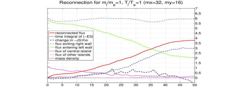
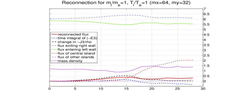
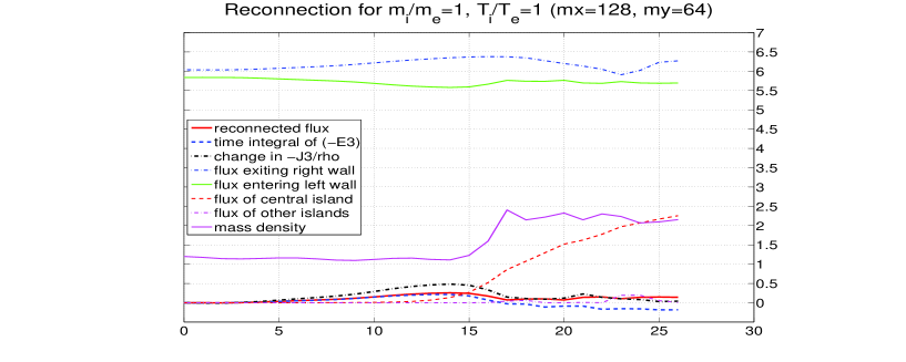
Figure 1. Three plots attempting to show convergence of reconnection data for electron-positron plasma with equal initial temperatures. Reconnection is suppressed for finer mesh resolution but fast reconnection occurs for coarse mesh resolution. We conjecture that numerical diffusion coupled with the ion inertial term is sufficient to admit fast reconnection. The appearance of a large central magnetic island beginning around time 15 is curious.

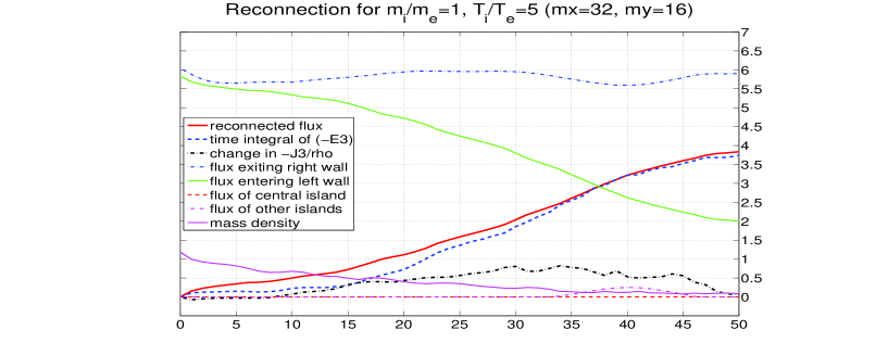
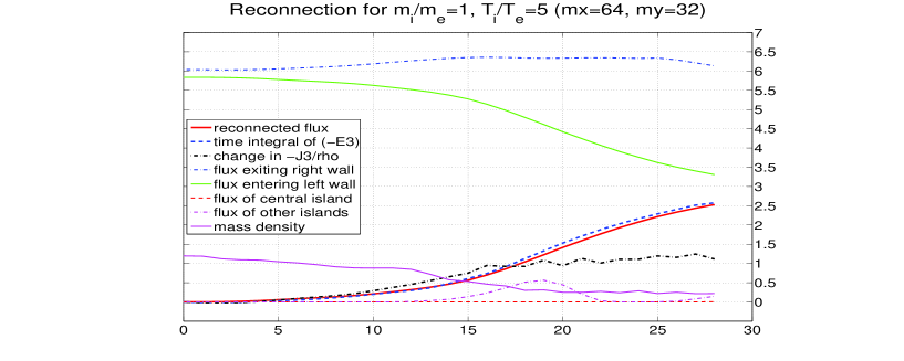
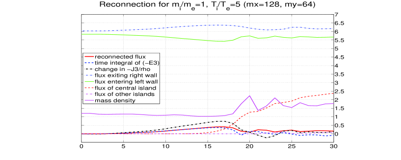
Figure 2. Convergence study of reconnection for electron-positron plasma with initial temperature ratio of 5. The reconnection rate would appear to decrease with decreasing numerical diffusion. Only for the finest mesh does a central magnetic island form.

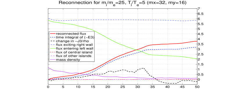
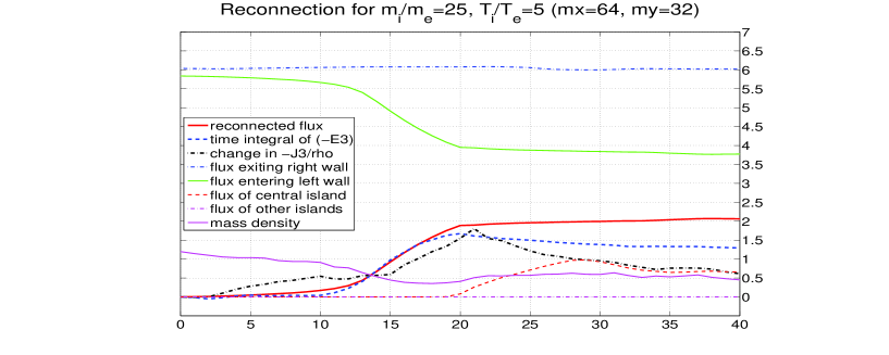
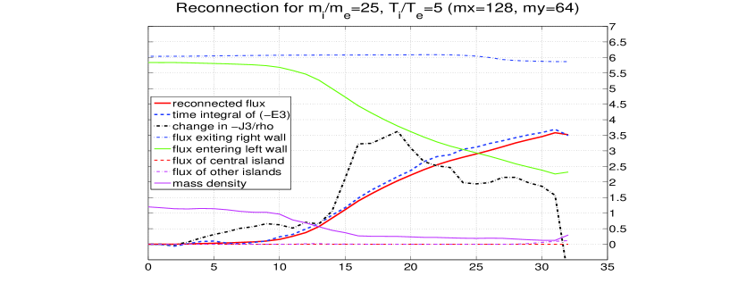
Figure 3. Convergence study of reconnection for electron-positron plasma with mass ratio of 25 and initial temperature ratio of 5. Fast reconnection occurs for both coarse and fine mesh resolutions. The anomalously early cessation of reconnection in the simulation at intermediate resolution is evidently related to the appearance of a large central magnetic island beginning around time 20.

References

- [1] N. Bessho, A. Bhattacharjee. Collisionless reconnection in an electron-positron plasma. Physical Review Letters, 95, 245001 (2005).
- [2] by same authorN. Bessho, A. Bhattacharjee. Fast collisionless reconnection in electron-positron plasmas. Physics of Plasmas, 14, 056503 (2007).
- [3] J. Birn, J.F. Drake, M.A. Shay, B.N. Rogers, R.E. Denton, M. Hesse, M. Kuznetsova, Z.W. Ma, A. Bhattacharjee, A. Otto, and P.L. Pritchett. Geospace environmental modeling (GEM) magnetic reconnection challenge. Journal of Geophysical Research – Space Physics, 106:3715–3719, 2001.
- [4] A.H. Hakim. Extended MHD modelling with the ten-moment equations. J. Fusion Energy, 27:36–43, 2008.
- [5] A. Hakim, J. Loverich, and U. Shumlak. A high-resolution wave propagation scheme for ideal two-fluid plasma equations. J. Comp. Phys., 219:418–442, 2006.
- [6] E.N. Parker. Sweet’s mechanism for merging magnetic fields in conducting fluids. J. Geophys. Res., 62:509–520, 1957.
- [7] E. Priest and T. Forbes. Magnetic Reconnection: MHD Theory and Applications. Cambridge University Press, 2007.
- [8] U. Shumlak and J. Loverich. Approximate Riemann solver for the two-fluid plasma model. J. Comp. Phys., 187:620–638, 2003.
- [9] P.A. Sweet. The neutral point theory of solar flares. In Electromagnetic Phenomena in Cosmical Plasmas, pages 123–134. Cambridge University Press, 1958.