Carbon isotope fractionation in protoplanetary disks

Abstract

We investigate the gas-phase and grain-surface chemistry in the inner 30 AU of a typical protoplanetary disk using a new model which calculates the gas temperature by solving the gas heating and cooling balance and which has an improved treatment of the UV radiation field. We discuss inner-disk chemistry in general, obtaining excellent agreement with recent observations which have probed the material in the inner regions of protoplanetary disks. We also apply our model to study the isotopic fractionation of carbon. Results show that the fractionation ratio, ¹²C/¹³C, of the system varies with radius and height in the disk. Different behaviour is seen in the fractionation of different species. We compare our results with ¹²C/¹³C ratios in the Solar System comets, and find a stark contrast, indicative of reprocessing.

1 Introduction

Studying the chemistry of the inner regions of protoplanetary disks (PPDs) is a step into the unknown. Until recently observations of molecules in PPDs could not probe the warmer, inner regions of the disk where planets form. Detections of CO, HCO⁺, H₂CO, C₂H, CS, SiO, HNC, CN and HCN (Dutrey et al. 1997; Kastner et al. 1997; Qi et al. 2003; Thi et al. 2004; Semenov et al. 2005) at millimetre wavelengths can only tell us about the physics and chemistry in the cold conditions at radii greater than $\sim$50 AU because of the limits of millimetre-wave sensitivity and spatial resolution. We have to go to the infrared to investigate the hotter material, and there comparatively few molecules have been seen. Initially H₂, CO (Najita et al. 2003; Brittain et al. 2003; Blake & Boogert 2004) and H₂O (Carr et al. 2004) were detected. Recently, the Spitzer Space Telescope has added OH, C₂H₂, CO₂ and HCN to the tally (Carr & Najita 2008; Lahuis et al. 2006) and a few detections of very large polycyclic aromatic hydrocarbon (PAH) molecules have been made (Geers et al. 2006). The Keck Interferometer has also brought us detections of hot HCN and C₂H₂ (Gibb et al. 2007). The regions of the disk close to the star are of immense interest because they are where terrestrial (and larger) planets begin to form, as well as comets. Molecules in the inner 30 or 40 AU could be the building blocks of the kinds of pre-biotic and biotic molecules we see in the Solar System today.

In the absence of observational evidence, we are left with theoretical work. This is valuable in its own right for understanding the processes in these regions, and for predicting observations for future proposals and even future technologies, such as ALMA, which will be able to probe these hidden inner disks. Previous modelling attempts of these very inner regions of PPDs (R$<$10 AU) have been few (Markwick et al. 2002; Millar et al. 2003; Ilgner et al. 2004; Ilgner & Nelson 2006; Agúndez et al. 2008), but have shown that these inner regions of PPDs are rich in molecules, including some complex molecules, such as benzene (Woods & Willacy 2007).

In this paper we present chemical models of a protoplanetary T Tauri-stage disk and a Minimum Mass Solar Nebula (MMSN), paying particular attention to the fractionation of carbon-bearing species. The fractionation in a particular molecule is defined as the abundance of the ¹²C-bearing variant over the ¹³C-bearing variant. Fractionation in carbon gives us a method of labelling: identifying, for instance, different regions of the disk and also identifying the different evolutionary processes involved in the formation of the disk – each process leaves its isotopic signature. Thus initially we study a typical protoplanetary disk, the physical aspects of which are explained in Sect. 2. We include a treatment of gas heating and cooling, which is expanded upon fully in Appendix A. In Sect. 3 we give a description of the chemical network, and the various chemical and photo-fractionation mechanisms including isotope-exchange reactions. Finally, we present our findings on carbon fractionation in protoplanetary disks, and set our results in both a Solar System and interstellar context.

2 The disk model: Physics

In order to accurately model a PPD one has to take into account many physical and chemical processes. One needs a thorough understanding of disk hydrodynamics and magnetohydrodynamics, turbulence, accretion, stellar spectrum, thermal balance, radiation transport, chemical composition, dust composition, etc. Whilst there are efforts to understand disks comprehensively and to model them accordingly with the appropriate feedback and interactions, such models are computationally very expensive and are very limited in their extent (e.g., Turner et al. 2007). Thus simplifications are often made, effectively decoupling different elements of the situation.

A major simplification is the separation of chemistry and physics when solving the equations of hydrodynamics for the disk temperature and density structure. In order to make the problem tractable a static hydrodynamic disk model is used to provide densities and dust temperatures throughout the disk. From this the UV photon distribution can be calculated (e.g., van Zadelhoff et al. 2003), assuming contributions to the UV field from the stellar source and the interstellar medium. Few models have been developed that determine the structure of the disk and the radiative transfer self-consistently (e.g., Nomura 2002; Millar et al. 2003). The final parameter required is that of the gas temperature. Some models (e.g., Markwick et al. 2002) have assumed that the gas and dust temperatures are identical but this significantly underestimates the gas temperature in the disk surface (Kamp & Dullemond 2004). We calculate the gas temperature in the disk from the density and dust temperature profiles using a heating-cooling balance technique. This is a simpler approach than a finding a self-consistent solution (see Aikawa & Nomura 2006, for example), but neglects the feedback interaction between changes in the gas temperature and gas density. Once all the physical parameters have been determined they can be used as inputs for the chemical model.

In reality, protoplanetary disks are not static: there is the large-scale motion of material accreting onto the star. There are also convective motions, often parameterised into vertical mixing motions and radial mixing motions. On all scales there is turbulence, which is mostly likely driven by magnetic fields in the disk. Turbulence drives mixing in both radial and vertical directions and models of mixing in the inner (Ilgner et al. 2004) and outer disk (Willacy et al. 2006; Semenov et al. 2006) have shown this to be important. Material will also be gradually accreted radially towards the central star. Here we ignore turbulent mixing but mimic the accretion flow of material moving toward the star by moving a number of parcels of gas from the outer edge of the model at 35 AU inward, along lines of constant scaleheight ($z_{h}$). These parcels are spaced vertically in 0.1$z_{h}$ intervals above the midplane of the disk, and we assume axisymmetry about the midplane. Each parcel will flow into the star in a time which can be derived from the principle of mass conservation. The radial velocity is given by:

$$v_{\mathrm{r}}=\frac{\dot{M}}{2\pi\Sigma R}\qquad R\gg R_{\star}$$ (1)

with $R$, the radius, $\dot{M}$, the accretion rate and $\Sigma$, the surface density of the disk. The accretion timescale, $\Delta t$, is approximately $\Delta R$/$v_{\mathrm{r}}$. Thus,

$$\Delta t\sim\frac{2\pi\Sigma R\Delta R}{\dot{M}}.$$ (2)

$\Sigma$ scales with 1/$R$ fairly closely for R$>$10 AU (D’Alessio et al. 2001; Andrews & Williams 2007), and so Eq. 2 only has a small dependence on $R$. A parcel starting at 35 AU will pass into the star in a time of approximately 0.41 Myr. In our framework of seventy radial points with a spacing of 0.5 AU, each parcel will spend $\approx$6 000 yr at each radial gridpoint before it is moved inwards. This simplistic method has been treated in more detail, for instance, in Aikawa et al. (1999, eq. (10)).

2.1 Disk structure

To determine the physical structure of the disk we use a model kindly supplied to us by Paola D’Alessio and based on D’Alessio et al. (1999, 2001), which models a flared disk using the $\alpha$-formulation (Shakura & Syunyaev 1973). The model has a central star with a temperature ($T_{\star}$) of 4 000 K, a mass ($M_{\star}$) of 0.7 M_⊙, a luminosity ($L_{\star}$) of 0.9 L_⊙, and a radius ($R_{\star}$) of 2.5 R_⊙ (c.f., Gullbring et al. 1998). The mass accretion rate ($\dot{M}$) is 10^-8 M_⊙ yr^-1. The viscosity parameter, $\alpha$=0.01. The dust in the disk has an ISM size distribution (Draine & Lee 1984) and is assumed to be well-mixed with the gas. The dust disk extends from $\sim$0.1 AU to 300 AU and has a mass of 0.032 M_⊙. The model provides the density and grain temperature. The gas temperature is calculated separately, and details are given in the following section.

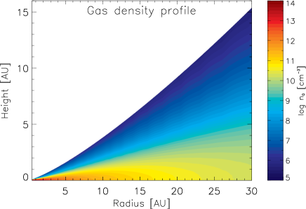
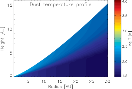
Figure 1: Gas density and dust temperature profiles from the models of Paola D’Alessio, re-gridded to our 35$\times$16 AU grid, spaced at 0.5$\times$0.02 AU.

From this model we have calculated a gas pressure scaleheight ($z_{h}$) for the disk based on the distance over which the density drops to the 0.01% level. The radial dependence of $z_{h}$ can be fit by a power law:

$$z_{h}=0.0337R^{14/11}.$$ (3)

Our chemical calculations extend from the midplane up to 6 $z_{h}$.

2.2 Gas and dust temperature

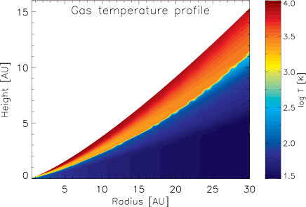
Figure 2: Results of the gas temperature determination for the inner 30 AU of the disk model. The slight “wobble” in the transition from the cold disk interior to the hot surface layers is due to a change from bare to mantled grains, which affects the heating due to H₂ formation (Sect. 4.1).

Table 1: Gas heating and cooling mechanisms included.

Mechanism	Reference(s)	Notes
Heating
Photoelectric effect	Kamp & van Zadelhoff (2001)	For silicate grains
$\cdots$	Bakes & Tielens (1994)	For small graphite and PAH grains
H2 collisional de-excitation	Kamp & van Zadelhoff (2001)	$\cdots$
H2 photodissociation	Kamp & van Zadelhoff (2001)	$\cdots$
H2 formation	Kamp & Dullemond (2004)	$\cdots$
$\cdots$	Cazaux & Tielens (2002b, 2004)	H2 formation efficiency
C ionisation	Tielens & Hollenbach (1985)	$\cdots$
Cosmic rays	Kamp & van Zadelhoff (2001)	For $\Sigma<$150g cm-2
$\cdots$	$\cdots$	(Umebayashi & Nakano 1981)
Stellar X-rays	Gorti & Hollenbach (2004)	X-ray ionisation rate
$\cdots$	Shang et al. (2002)	Secondary effect
Cooling
Oi fine structure lines	Tielens & Hollenbach (1985)	$\cdots$
$\cdots$	Kamp & van Zadelhoff (2001)	Molecular line data
Ci fine structure lines	Tielens & Hollenbach (1985)	$\cdots$
$\cdots$	Kamp & van Zadelhoff (2001)	Molecular line data
Cii line at 157.7 $\mu$m	Tielens & Hollenbach (1985)	$\cdots$
$\cdots$	Kamp & van Zadelhoff (2001)	Molecular line data
1D line of Oi at 6300 Å	Tielens & Hollenbach (1985)	$\cdots$
$\cdots$	Sternberg & Dalgarno (1989)	Electron impact excitation
H2 rovibrational lines	Le Bourlot et al. (1999)	$\cdots$
CO rotational lines	Tielens & Hollenbach (1985)	$\cdots$
$\cdots$	Kamp & van Zadelhoff (2001)	Molecular line data
CH rotational lines	Kamp & van Zadelhoff (2001)	$\cdots$
Lyman-$\alpha$ line	Kamp & van Zadelhoff (2001)	$\cdots$
Gas-grain collisions	Kamp & van Zadelhoff (2001)	$\cdots$

Until fairly recently PPD models assumed that the gas portion of the disk is in thermal equilibrium with the dust throughout its entirety (e.g., Markwick et al. 2002) . This can often be an underestimate of the gas temperature in regions of the disk close to the central radiation source, and especially in the tenuous surface which is exposed to the interstellar radiation field (ISRF), where conditions are similar to a photon-dominated region (PDR). This assumption can underestimate the gas temperature by an order of magnitude (Kamp & Dullemond 2004).

In an effort to more accurately model the isotope chemistry in PPDs, for which gas temperature is an important factor (see Sect. 3.1), we have calculated the gas temperature separately from the dust temperature, by balancing heating and cooling terms. Several authors have previously taken this approach (Kamp & van Zadelhoff 2001; Kamp & Dullemond 2004; Gorti & Hollenbach 2004; Tielens & Hollenbach 1985) and we follow the prescriptions given in their papers, adapting them to T Tauri disks where necessary (see Table 1 for details).

We take into account seven mechanisms which affect the gas heating rate in the disk – the photoelectric effect ($\Gamma_{\mathrm{PE}}$), collisional de-excitation of H₂ ($\Gamma_{\mathrm{CDx}}$), photodissociation of H₂ ($\Gamma_{\mathrm{Phd}}$), formation of H₂ ($\Gamma_{\mathrm{Form}}$), ionisation of C ($\Gamma_{\mathrm{CIon}}$), cosmic rays ($\Gamma_{\mathrm{C-ray}}$), and stellar X-rays ($\Gamma_{\mathrm{X-ray}}$). Gas-grain collisions can also act as a heating mechanism when the dust temperature exceeds the gas temperature. However, since this rarely happens in the disk model, gas-grain collisions act mostly as a cooling mechanism ($\Lambda_{\mathrm{G-G}}$). Other cooling mechanisms included are: the fine-structure lines of atomic oxygen at 63.2, 145.6 and 44.0 $\mu$m ($\Lambda_{\mathrm{O}\textsc{i}}$), the fine-structure lines of atomic carbon at 609.2, 229.9 and 369.0 $\mu$m ($\Lambda_{\mathrm{C}\textsc{i}}$), the 157.7 $\mu$m line of singly-ionised carbon ($\Lambda_{\mathrm{C}\textsc{ii}}$), the metastable ¹D line of atomic oxygen at 6300 Å  ($\Lambda_{\mathrm{O6300}}$), rovibrational lines of H₂ ($\Lambda_{\mathrm{H_{2}}}$), 25 rotational lines of CO ($\Lambda_{\mathrm{CO}}$), rotational cooling of the CH radical ($\Lambda_{\mathrm{CH}}$) and Lyman-$\alpha$ cooling ($\Lambda_{\mathrm{Ly\alpha}}$). Further details are given in Appendix A.

Thus the temperature of the gas is calculated by balancing the heating and cooling rates. We use the modified Brent’s method of root-finding to solve for the gas temperature, as found in Press et al. (1992). This method works well in regions where the gas temperature function is continuous. Results of the gas temperature calculation are shown in Fig. 2.

To increase computational efficiency we only perform this calculation once at every grid point, rather than iterating to a solution. Thus the gas temperature is calculated first using chemical abundances from the previous gridpoint and the new temperature used to calculate the chemical reaction rates for the current grid point. This is acceptable since there is only a weak coupling between the gas temperature calculation and the chemistry: any changes in temperature in response to a small change in chemistry will be small, and vice versa.

2.3 Radiative transfer

Protoplanetary disks are subject to radiation from the central stellar source and from the ISRF. In order to calculate the UV radiation field at any one point in our disk model, we make use of the direct/diffuse treatment of FUV photons from Richling & Yorke (2000). We include the effects of radiation from both the central protostar and from the external UV field, and also include the effects of scattering of photons by dust grains. Absorption and scattering coefficients are based on the work of Draine & Lee (1984) and Preibisch et al. (1993), who assume a mixture of silicates, amorphous carbons and dirty ice-coated silicate grains. The disk is divided up into square cells ($\Delta z$=$\Delta r$=0.02 AU) and the radiative transfer equation is solved separately for both sources of radiation, and for the direct and diffuse (scattered) components of each UV radiation field (see Richling & Yorke 2000, for details). The total UV flux at a given point is the sum of the contributions from the stellar and interstellar UV fields, that is, we employ a 1+1D approach rather than the full 2D treatment calculated by Richling & Yorke (2000).

The radiative transfer code is not able to account for the difference between the shape of the interstellar UV field and that generated by the spectrum of the young star. Observations have shown that T Tauri stellar fields are different to the interstellar radiation field, and can be dominated by strong emission features (such as Lyman-$\alpha$). This can significantly impact the chemistry of the surface layers of the disk since Lyman-$\alpha$ can dissociate some molecules, such as OH and CH₄, and not others. Bergin et al. (2003) found that this effect can account for high CN/HCN ratios observed in some disks (Dutrey et al. 1997; Kastner et al. 1997). The strength of the T Tauri stellar radiation field has been estimated from FUSE observations as a few hundred times G₀ at a radius of 100 AU (Bergin et al. 2003), where G₀ is the standard interstellar radiation field strength. Here we adopt a value of 500 G₀ at a radius of 100 AU.

We also calculate photoionisation by X-rays assuming an X-ray luminosity of $10^{-4}$ L_⋆ (Gorti & Hollenbach 2004) or $9\times 10^{-5}$ L_⊙. The calculation of the X-ray photoionisation rate is described in more detail in Sec. 3.2 and the contribution of X-ray heating to the gas temperature is discussed in Appendix A.1.

2.4 Self-shielding

Self-shielding by the abundant molecules H₂ and CO moderates the effect of photodissociation. We incorporate this mechanism into our model by using the “shielding factor” approach of van Dishoeck & Black (1988) and Lee et al. (1996). For CO we use the data of van Dishoeck & Black (1988, see Sect. 3.1.2 for more detail), and for H₂, Lee et al. (1996). These papers deal with interstellar clouds, for which the turbulent line width can be larger than the thermal line widths in PPDs. We use the re-normalisation technique proposed by Aikawa & Herbst (1999) to account for this difference, where the column density of H₂ used in the self-shielding calculation is reduced by the factor $c_{S}$/3 km s^-1 (where $c_{S}$ is the sound speed of the gas, and 3 km s^-1 is the turbulent line width assumed in the cited self-shielding calculations, for the ISM). In the inner disk, where the temperature and the sound speed are highest, this has less effect than that found by Aikawa & Herbst (1999) in the outer disk.

We follow Aikawa & Herbst (1999) in assuming that H₂ and CO are only dissociated by the ISRF and not by stellar UV because of the difficulty of solving the equation of radiative transfer simultaneously in two dimensions. The stellar radiation is only effective in the relatively low density surface regions (above z/R$\sim$0.3, or 3.5 $z_{h}$ at R=30 AU), and thus has little effect on the chemistry in the molecular regions we wish to study.

3 The disk model: Chemistry

3.1 Isotopes of carbon

Our knowledge of the chemistry of ¹³C-bearing species stems from 30 years ago, and has advanced little since. This makes it difficult to accurately study a system which includes ¹³C-bearing species because reaction rates are simply not known. There is some data available on differences in the zero-point energy between ¹²C- and ¹³C-bearing species, but not for all species, and the Kinetic Isotope Effect (KIE) has been used in theoretical work by some (e.g., Young 2006) to account for the differences in molecular mass, but this effect is complicated by the actual mechanism of reaction, i.e., the KIE only applies when the bond being broken/created is a bond between ¹³C and another atom. However, there are two mechanisms which are known to fractionate carbon isotopes – fractionation through chemical exchanges, and through photodissociation.

3.1.1 Fractionation through chemical exchange reactions

Smith & Adams (1980) performed laboratory studies of isotope exchange reactions, and revealed that the most important reaction for exchanging carbon isotopes is:

$$\mathrm{{}^{13}C^{+}+^{12}CO\rightleftharpoons^{13}CO+^{12}C^{+}+}\Delta E,$$ (4)

as predicted by Watson et al. (1976). $\Delta E$ is the zero-point energy difference between the reactants and products, and is taken to be 35 K for this reaction. This small energy difference makes the forward reaction more efficient at low temperatures. The rate of this reaction was initially measured by Watson et al. (1976) at 300 K, and at 80, 200, 300 and 510 K by Smith & Adams (1980). Langer et al. (1984) then calculated rates down to 5 K. A more recent calculation by Lohr (1998) produced rates from 10-1 000 K, in reasonable agreement with both Smith & Adams (1980) and Langer et al. (1984). The difference in the forward and backward rates of Eq. 4 is small, but it is still discernible even at 300 K (Smith & Adams 1980).

Smith & Adams (1980) also measured the rate of another isotope-exchange reaction at the same temperatures as before:

$$\mathrm{H^{12}CO^{+}+^{13}CO\rightleftharpoons H^{13}CO^{+}+^{12}CO+}\Delta E,$$ (5)

with $\Delta E$=9 K (Langer et al. 1984). This is only effective at very low temperatures, with virtually no difference in forward and backward rates at 300 K and only a small difference at 80 K (Smith & Adams 1980). Langer et al. (1984) calculated rates over the range 5–300 K and Lohr (1998) made rate calculations over 10–1 000 K.

Other exchange reactions similar to Eqs. (4) and (5) may occur. However, a chemical reaction will almost certainly dominate over an exchange reaction such as reactions (4) or (5) except when it is energetically unfavourable to do so (due to complicated structural rearrangement, for instance). In practice, many molecules react chemically with C⁺, for example, rather than undergo carbon exchange. An exception to this is CS, for which $\Delta E\approx$26 K in the reaction (Watson et al. 1976). Another is CH₃ (Dalgarno & Black 1976). Lohr (1998) suggests that the reaction between HOC⁺ and CO might be important for isotope exchange since it moves in the opposite way to the exchange involving HCO⁺ (Eq. 5), preferentially putting ¹³C into CO. The difference in zero point energies is small, 2.5 K. Similarly, Langer (1992) suggested the importance of the possible exchange between C⁺ and CN, which might compete with the photodestruction of CN in the upper layers of disks. The difference in zero point energy is 34 K. However, none of the rates of these exchange reactions have been measured or calculated to our knowledge, and we do not include them in our model.

For convenience, we have fit both the forward and backward reaction rates for reactions (4) and (5) given in the literature with a smooth function in the standard form. Thus for reaction (4),

$$k_{\mathrm{for}} = 3.3\times 10^{-10}\left(\frac{T}{300\,\mathrm{K}}\right)^{-0.448}~{}\qquad\mathrm{cm^{3}s^{-1}}$$ (6)

$$k_{\mathrm{rev}} = k_{\mathrm{for}}\exp(-35\,\mathrm{K}/T)\qquad\qquad\qquad\mathrm{cm^{3}s^{-1}}$$ (7)

and for reaction (5),

$$k_{\mathrm{for}} = 2.6\times 10^{-10}\left(\frac{T}{300\,\mathrm{K}}\right)^{-0.277}~{}\qquad\mathrm{cm^{3}s^{-1}}$$ (8)

$$k_{\mathrm{rev}} = k_{\mathrm{for}}\exp(-9\,\mathrm{K}/T)\qquad\qquad\qquad\mathrm{cm^{3}s^{-1}}$$ (9)

These fits are in excellent agreement with both the experimental results of Smith & Adams (1980, agree to within 7%) and the calculations of Langer et al. (1984, 3%) and Lohr (1998, 8% above 50 K).

3.1.2 Fractionation through photodissociation

Carbon monoxide is dissociated mostly via line absorption and thus as the column density of carbon monoxide towards the emitter increases, so the absorption line saturates as photons are absorbed by the intervening material. At some point, a carbon monoxide molecule becomes shielded from dissociation by the presence of other molecules along the line of sight – not only molecules of the same kind, but also isotopologues and atomic and molecular hydrogen, whose dissociation bands may overlap. The degree of self-shielding depends on this overlap, and thus the shielding of ¹³CO, say, will depend on the column density of ¹²CO and H₂, as well as that of ¹³CO. One must also take into account the attenuation provided by dust grains.

This complex situation has been simplified by a number of authors for different situations. van Dishoeck & Black (1988) treat ¹³CO explicitly, and therefore we use their treatment in our model. They have tabulated “shielding factors” which modify the photodissociation rate according to the factors detailed above. These shielding factors depend primarily on the column densities of ¹²CO and H₂, with the other factors (including the isotope ratio) remaining fixed. Since we calculate the column density of ¹³CO in our model (and this differs from the fixed value of $N(^{12}$CO)/$N(^{13}$CO)=45 used in van Dishoeck & Black 1988), we assume $N(^{12}$CO)=45$\times N(^{13}$CO) for the purpose of calculating the shielding factor for ¹³CO only. In general, $N(^{12}$CO)/$N(^{13}$CO) is less than 45, and so we may be slightly overestimating the contribution made to the self-shielding of ¹³CO by ¹²CO.

For given column densities of ¹²CO and H₂, ¹³CO is shielded less than ¹²CO, and thus is preferentially photodissociated. So as one proceeds from a region of high extinction to a region of low extinction, one would see ¹³CO being photodissociated where ¹²CO is already self-shielded, and hence an increase in the fractionation ratio, ¹²CO/¹³CO, in this region. This effect can be seen observationally at the edges of molecular clouds (e.g., Sheffer et al. 1992).

This situation is complicated further by some recent preliminary work showing that self-shielding is temperature dependent (Lyons et al. 2007). Since the predissociation bands for H₂ and CO are thermally broadened and there is the possibility of overlap with adjacent electronic states, additional CO vibrational bands have to be considered at high temperatures. This work will be particularly applicable to the temperatures found in PPDs, and we look forward to the results of these investigations.

3.1.3 Interstellar and Solar System context

The isotope ratio for carbon (¹²C/¹³C) in the Solar System is widely accepted to be 89 (Anders & Grevesse 1989; Clayton & Nittler 2004; Meibom et al. 2007), although recent measurements of the solar photosphere have indicated a ratio of 80$\pm$1 (Ayres et al. 2006). This is greater than in the local interstellar medium (ISM), where the value is taken to be 77 (Wilson & Rood 1994), greater than the Orion Bar region (¹²C/¹³C$\sim$60; Keene et al. 1998; Langer & Penzias 1990), and much greater than the Galactic Centre (¹²C/¹³C$\sim$20; Milam et al. 2005; Langer et al. 1984). This galactic gradient (Langer & Penzias 1990) is due to the higher star formation rate in the inner Galaxy (Tosi 1982), where the fraction of ¹³C has been enhanced by the ¹³C-rich ejecta of evolved, intermediate-mass stars (Iben & Renzini 1983) in the time since the formation of the Solar System.

Wilson & Rood (1994) give a numerical evaluation of how the isotope ratio changes with galactocentric distance. Since the Sun formed approximately 1.9 kpc closer to the Galactic Centre (Wielen et al. 1996) than its present location (7.94 kpc, Eisenhauer et al. 2003), presumably it would have formed in a region with a lower ¹²C/¹³C ratio, viz., $\approx$67, ignoring temporal evolution. Wielen & Wilson (1997) discuss a method of incorporating the temporal evolution of the ISM, and derive a value of 62 for the region and time period in which the Solar System condensed. The large difference between this value and the present Solar System value of 89 indicates that the Solar System must have become either significantly enriched in ¹²C, or there must have been a significant depletion of ¹³C. Recent studies of iron isotopes in the Solar System have indicated that the Sun most likely formed close to one or more massive stars (Hester et al. 2004), which produce ¹²C in the triple-$\alpha$ reaction in their interiors (Timmes et al. 1995). These stars, which go on to form Type II supernovae, may have contaminated the solar protoplanetary nebula with ¹²C-rich material during its formation. Alternative explanations for this difference in isotope ratios are X-ray flares (Feigelson et al. 2002), cloud mergers, orbital diffusion or radial gas streaming (see Milam et al. 2005, for further details). It seems unlikely that the increase in the ¹²C/¹³C ratio above the interstellar value is due to the processing of material once the Solar System had been established (Lecluse et al. 1998).

In light of these factors, we choose an initial ¹²C/¹³C ratio of 77, between the values of 62 and 89, in line with that of the present-day ISM ratio. The value of this ratio is not crucial to the chemistry, and similar fractionation levels are obtained for the entire range of values, 62–89.

3.2 The reaction set

Table 2: Initial fractional abundances for abundant carbon-bearing species. These abundances are the result of 1 Myr in a molecular cloud model

Species		Gas phase		12CX/13CX		Solid phase		g–12CX/g–13CX
C2		1.7 (-7)		169		negligible		–
C3H2		4.1 (-7)		160		1.9 (-6)		133
C2H2		3.6 (-7)		153		1.2 (-6)		141
C4H		5.3 (-7)		152		negligible		–
HCN		2.4 (-8)		152		3.7 (-6)		111
HC3N		1.1 (-7)		150		5.8 (-7)		134
CN		1.3 (-7)		146		negligible		–
HNC		1.0 (-8)		144		2.6 (-7)		106
C4		7.2 (-8)		144		negligible		–
C3		9.8 (-8)		134		negligible		–
C3H		5.3 (-7)		133		negligible		–
C4H2		9.6 (-9)		133		8.5 (-7)		136
C2H		6.5 (-8)		118		negligible		–
CH		2.4 (-8)		113		negligible		–
CH3		4.8 (-8)		107		negligible		–
H2CO		4.7 (-8)		107		2.1 (-7)		106
CH4		2.3 (-6)		102		9.2 (-6)		99
C		1.1 (-7)		93		negligible		–
CO		3.1 (-5)		55		2.6 (-6)		55
CO2		1.7 (-7)		51		6.4 (-7)		55

Note. — $x$ ($-y$) here represents $x\times 10^{-y}$. Isotope ratios for species with more than one carbon atom are calculated by dividing the total abundance of ¹²C by the total abundance of ¹³C in that particular molecule. Other species of note, and their initial fractional abundances: H₂ 5.0$\times$10^-1, He 1.4$\times$10^-1, g–H₂O 1.4$\times$10^-4, H 2.5$\times$10^-5, g–NH₃ 1.6$\times$10^-5, O 1.4$\times$10^-6, OH 6.4$\times$10^-7.

The chemical reaction network is based on the UMIST99 gas-phase ratefile (Le Teuff et al. 2000), with two additions:

1) we include grain surface reactions from Hasegawa & Herbst (1993) and Hasegawa et al. (1992). We consider cosmic ray heating and thermal desorption, with updated binding energies from Bisschop et al. (2006), Öberg et al. (2005) and Fraser et al. (2001). For atomic H, we use updated binding energies from Cazaux & Tielens (2004, 2002b), who treat physisorption and chemisorption onto grains distinctly, with binding energies $E_{\mathrm{H_{p}}}$=600 K and $E_{\mathrm{H_{c}}}$=10 000 K, respectively. In our calculations we assume that the sticking coefficient of H is 0.4, and that for all other species is 0.3.

2) we include a simple treatment of X-ray chemistry similar to that by Gorti & Hollenbach (2004), i.e., we calculate an ionisation rate per atom, which depends on photon flux and cross-section:

$$\zeta_{\mathrm{X}}^{i}=6.25\times 10^{8}\int_{0.5}^{10}\sigma_{\mathrm{X}}^{i}(E)\frac{F(E)}{E}\exp(-\tau_{\mathrm{X}}(E))dE\quad\mathrm{s^{-1}},$$ (10)

for atom $i$. Fits to X-ray cross-sections ($\sigma_{\mathrm{X}}^{i}$) for astrophysically relevant molecules are taken from Verner & Yakovlev (1995). $F(E)$ is the X-ray photon flux at a radius R, as a function of energy 0.5$<E<$10 keV. $\tau_{\mathrm{X}}(E)=N_{0}\sigma_{\mathrm{X}}(E)$ is the X-ray extinction due to a column density $N_{0}$. We assume that X-ray ionisation leads to the loss of a single election, and that the ionisation rate for molecules is the sum of the rates for the constituent atoms. See Aikawa & Herbst (2001) for a more detailed treatment of X-ray chemistry.

In total, our reaction network comprises 475 gas and grain species, and over 8 000 gas-phase and surface reactions. More than three-quarters of these reactions involve ¹³C. There have been recent observations (Sakai et al. 2007; Takano et al. 1998) of ¹³C isotopologues and isotopomers which show that there may be differing properties for carbon atoms attached in different places in the molecule. However, due to a dearth of experimental data on how ¹³C-bearing species react in comparison to ¹²C-bearing species, we have assumed that reactions involving ¹³C proceed at the same rate as their ¹²C counterparts. We have taken account of the increased number of reaction products which comes from the inclusion of isotopic species. For example, the reaction:

$$\rm C_{2}+H\longrightarrow\rm CH+C$$ (11)

with rate $k$ now becomes:

$$\rm{}^{12}C^{12}C+H \longrightarrow \rm{}^{12}CH+^{12}C$$ (12)

$$\rm{}^{12}C^{13}C+H \longrightarrow \rm{}^{12}CH+^{13}C$$ (13)

$$\rm{}^{12}C^{13}C+H \longrightarrow \rm{}^{13}CH+^{12}C$$ (14)

$$\rm{}^{13}C^{13}C+H \longrightarrow \rm{}^{13}CH+^{13}C,$$ (15)

with rates $k$, $k$/2, $k$/2 and $k$, respectively. We preserve functional groups such that, e.g.,

$$\rm{}^{13}CH_{3}^{12}CN+He^{+} \longrightarrow \rm{}^{12}CN+^{13}CH_{3}^{+}+He$$ (16)

$$\rm{}^{13}CH_{3}^{12}CN+He^{+} \mathop{\vbox{\hbox{\ooalign{\raise-0.43057pt\hbox{$\hbox{$\longrightarrow$\hskip 0.50003pt}$}\cr\cr$\hbox{\hskip 6.00006pt/}$}}}} \rm{}^{13}CN+^{12}CH_{3}^{+}+He$$ (20)

and we preserve double bonds in preference to single bonds:

$$\rm H_{2}^{13}CO+^{12}CH \longrightarrow \rm H^{13}CO+^{12}CH_{2}$$ (21)

$$\rm H_{2}^{13}CO+^{12}CH \mathop{\vbox{\hbox{\ooalign{\raise-0.43057pt\hbox{$\hbox{$\longrightarrow$\hskip 0.50003pt}$}\cr\cr$\hbox{\hskip 6.00006pt/}$}}}} \rm H^{12}CO+^{13}CH_{2}.$$ (25)

As initial fractional abundances we use the outputs of an interstellar (IS) cloud model ($n$=2$\times$10⁴ cm^-3, $T$=10 K, $A_{\mathrm{V}}$=10) which uses the same chemical network, and is allowed to run for 10⁶ yr. The inputs to this cloud model are the “low metal abundances ”of Graedel et al. (1982), viz. H:He:O:C:N:Si are 1:0.14:1.76$\times$10^-4:7.30$\times$10^-5:2.14$\times$10^-5:2.00$\times$10^-8. Our IS cloud model is a simple single-point approximation, but it reproduces the results of Langer & Graedel (1989) very well. We are in agreement to within a factor of 2 for important species such as CO, HCO⁺, O, CH, CH₂ and H₂CO, and a factor of five agreement with C⁺, C₂ and H₂O. There is a lesser agreement with CN, HCN, C₂H, CH₄ and OH due to the advances in the accuracy of reaction rate determination in the last 25 years. For instance, our model produces an overabundance (compared to Langer & Graedel 1989) of CN by a factor of $\sim$20, due to a faster rate for the reaction:

$$\rm CH+N\longrightarrow\rm CN+H.$$ (26)

Langer & Graedel (1989) use a rate of 4.5$\times$10^-12 cm³ s^-1 at 20 K, whereas the revised rate from Le Teuff et al. (2000) is 2.1$\times$10^-10 cm³ s^-1, 47 times faster. See Table 2 for input abundances for select species, and also the fractionation ratios after the molecular cloud stage.

The chemical fractionation which occurs in an interstellar cloud is explored in detail by Langer et al. (1984) and Langer & Graedel (1989). In summary, Langer et al. (1984) are able to classify C-bearing species into three families – CO, HCO⁺ and the “carbon isotope pool” – with distinct isotopic behaviours. The fractionation in CO is driven mainly by reaction (4), which favours the production of ¹³CO at the low temperatures and densities of interstellar clouds, driving the ¹²CO/¹³CO ratio down. The fractionation of HCO⁺ is driven both by reaction (5), which preferentially puts ¹³C into HCO⁺ at low temperatures, and also by its formation from elements of the carbon isotope pool, which are ¹²C-enriched. The fractionation in these remaining carbon-bearing molecules is driven to high ¹²C/¹³C ratios since the chemistry is based on C⁺, for which ¹²C⁺ is favoured at low temperatures (reaction 4) and much ¹³C is taken up in ¹³CO.

4 Results

4.1 Gas heating and cooling

The gas temperature in our model of a circumstellar disk can reach $\sim$8 000 K at the surface, vastly exceeding the temperature of the dust from the input dust models, which is a few hundred degrees in the same region. Such an effect has also been found by Kamp & van Zadelhoff (2001); Kamp & Dullemond (2004) and Glassgold et al. (2004) using different disk models. Clearly there is a strong need for disk models which calculate dust and gas temperatures individually. The gas and dust are not well coupled collisionally (and hence not in thermal equilibrium) in the disk surface, where the optical depth to the ISRF ($\tau$) is less than 0.5 ($\sim$3 $z_{h}$).

Heating by the photoelectric effect on small carbon and PAH grains is very important in the surface layers of the disk. This mechanism dominates almost all others in the upper third of the disk; gas heating due to H₂ formation becomes the most effective mechanism in a limited region where H₂ is photodissociated, around $z$=4–5$z_{h}$. Intermediate layers of the disk are heated mainly by X-ray heating for radii $\gtrsim$10 AU, and by gas-grain collisions inside of this radius. The midplane is heated predominantly by collisional de-excitation of H₂ molecules. The lower two-thirds of the disk are cooled mostly by molecules - in the most part, CO molecules are the most effective coolant, although CH molecules cool the midplane very efficiently at larger radii, R$\gtrsim$17 AU. In the upper third of the disk, cooling by the forbidden lines of Oi is very effective, with Lyman-$\alpha$ cooling dominating at the very surface of the disk, inside of 20 AU.

The transition between the hot surface layers and the cool bulk of the disk shows some small oscillations in temperature (Fig. 2). This is a result of the inclusion of icy grains, with a different H atom binding energy compared to bare grains in our model. On icy grains H atoms can only physisorb and therefore have a relatively short residence time. The oscillations occur in the region where the transition from bare to icy grains occur.

4.2 Fractionation of carbon isotopes

The disk can can be split into different regions depending on temperature, which is the dominating factor in the carbon fractionation of different species. The cold midplane region (“the cold region”, $T$=30–100 K) of the disk extends up to $\sim$3.5 $z_{h}$, which equates to 9 AU at a radius of 30 AU. In this region the majority of molecules are frozen out onto the surface of dust grains; only very volatile species (CO, CH₄) are in the gas phase. The warmer temperatures in the very inner part of the disk means that the ice line for water falls close to 2 AU.

Above the cold region is a transition region (“the transition region”, $T$=100–2 500 K), which generally has a thickness of $\sim$0.8 $z_{h}$ (2 AU at $R$=30 AU). The increase in temperature in this region causes molecules to evaporate from grain surfaces - H₂O is one of the last species to persist on grains. UV extinction is low enough for most molecules to be photoprocessed, although H₂, ¹²CO and ¹³CO remain shielded.

Lastly, the surface region (above $\sim$4.3 $z_{h}$) of the disk is heavily ionised and very hot (“the hot region”, $T$=2 500–8 000 K). Ionised species have a fractional abundance of $\sim$10^-3 in the surface region, indicating that most hydrogen is atomic and not yet ionised. These three regions are evident in Figs. 3 and 5. We will look at some characteristic species in detail and their properties in these three regions.

4.2.1 CO, HCO⁺ and CO₂

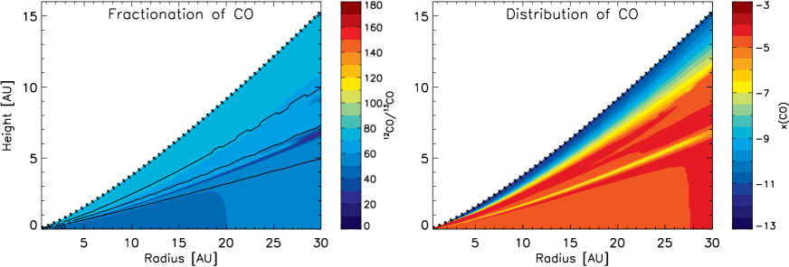
Figure 3: Carbon monoxide fractionation shown as the ratio of ¹²CO/¹³CO throughout the disk. Three different regions can be seen in the fractionation data - the hot region at the top of the disk, the cold region at the bottom and the transition region in between. The solid lines in this and following figures represent levels of optical depth to the ISRF, $\tau$=0.1, 1, 10. The dotted line indicates the designated surface of the disk at 6 $z_{h}$.

CO is an important species in disks since it is the dominant gas-phase molecule other than H₂ and can be used observationally to trace the bulk gas of the disk. It is also important because it can be used to trace the vertical temperature structure in disks, as in Guilloteau & Dutrey (1998); Dartois et al. (2003) and Piétu et al. (2007).

Of the CO introduced into the disk from the interstellar medium at 35 AU in our model, 92% of that is in the gas phase, and 8% is in the form of CO frozen onto dust grains. CO desorbs at low temperatures (26 K; Öberg et al. 2005) and in the inner disk temperatures are always above this, so CO quickly desorbs and very little ($\ll$1%) CO ice remains. Hence there is a high abundance of gaseous CO available to take part in chemical reactions.

The fractionation ratio of CO in the disk has a limited range, varying from 25-77 throughout the disk. This contrasts with observed ratios in diffuse interstellar clouds where there is a much wider range, 15$<$N(¹²CO)/N(¹³CO)$<$170 (Liszt 2007). The fractionation ratio of CO in the midplane does not change a great deal, 47–55 between 1 and 30 AU (Fig. 3). However its high abundance means it is able to be involved in exchange reactions thereby altering the fractionation of other molecules, e.g., HCO⁺, which shows an increase in fractionation with decreasing radius. This is a consequence of exchange reaction (5). Under the high density conditions of the disk, this process is roughly in chemical equilibrium:

$$k_{\mathrm{for}}n(\mathrm{H^{12}CO^{+}})n(\mathrm{{}^{13}CO}) = k_{\mathrm{rev}}n(\mathrm{H^{13}CO^{+}})n(\mathrm{{}^{12}CO})$$ (27)

$$\Rightarrow\frac{n(\mathrm{H^{12}CO^{+}})}{n(\mathrm{H^{13}CO^{+}})} = \exp{(-9\,\mathrm{K}/T)}\frac{n(\mathrm{{}^{12}CO})}{n(\mathrm{{}^{13}CO})}$$ (28)

using the relation in Eq. (9). Thus at temperatures of 32 K, where the ¹²CO/¹³CO ratio is 55, we should expect H¹²CO⁺/H¹³CO⁺=41, and at temperatures of 270 K, 45, as seen. Thus at higher temperatures (T$\gtrsim$60 K), the fractionation of HCO⁺ begins to trace the fractionation of CO, at least for the midplane region of the disk where CO is the only source of HCO⁺. The fractionation of HCO⁺ is shown in Fig. 4. Within 10 AU, HCO⁺ reacts with increasingly abundant hydrocarbons (e.g., C₃H₄, C₄H₂) and ammonia to create reactive ions and to reform CO, and within 8 AU these reactions become faster than the interchange between CO and HCO⁺.

Figure 4: The fractionation and distribution of the formyl ion, HCO⁺. White areas in this and subsequent figures indicate regions of negligible fractional abundance, $x$(X)$<$10^-13.

At radii of a few AU, the reaction between CO and OH is the major contributor to the formation of CO₂. This reaction has a moderate activation barrier, and thus proceeds more rapidly at higher temperatures. This reaction, which is important for both atmospheric and combustion chemistry, is one of the few for which mass-independent isotope effects have been investigated (c.f., Chen & Marcus 2005; Stephens et al. 1980; Smit et al. 1982; Roeckmann et al. 1998). These calculations and experiments find a small difference in the reaction rates of ¹²CO and ¹³CO with OH, but they were carried out at significantly higher pressures than are found in protoplanetary disks. At the lowest pressures considered, they found that the reaction involving ¹³CO is faster than that involving ¹²CO by less than 1%. Given that this percentage is dwarfed by the uncertainties in published reaction rates, the Kinetic Isotope Effect (of which this is an example) is unlikely to affect our results.

The fractionation ratio of CO ice in the midplane resembles that of gaseous CO. CO₂ ice, with a higher binding energy than CO ice, has a fractionation ratio which decreases from its input value of 55 to a value slightly higher than that of CO (46) in the very inner part of the disk, 49. The value of ¹²CO₂/¹³CO₂ ice ratio has been determined to be 81$\pm$11 in a young protostar, Elias 29 (catalog ) (Boogert et al. 2000a). This is unusually high, especially since the nascent cloud, $\rho$ Oph, shows ¹²C/¹³C ratios typical of the local ISM (Casassus et al. 2005; Bensch et al. 2001). This value is also somewhat higher than the ¹²CO/¹³CO ice ratio along the same line of sight, 71$\pm$15 (Boogert et al. 2002). A suggestion for this high value (Boogert et al. 2000b) is that CO₂ may have been formed from C⁽⁺⁾ rather than CO, as generally assumed. In our model, the vast majority of CO₂ ice comes from CO, in agreement with Ehrenfreund & Schutte (2000). Whatever the formation route, it seems that CO₂ ice ratios are determined in the parent cloud rather than the hot core around the protostar (Charnley et al. 2004).

Towards the top of the cold region in the disk ($z\sim$2.7 $z_{h}$) there is a layer of low abundance of CO. Above this layer, CO can be destroyed by reactions with He⁺, from the X-ray ionisation of He. Some carbon ions resulting from this destruction end up forming hydrocarbons on the surfaces of dust grains. At this height in the disk, the grain temperature is just high enough that hydrocarbons can thermally desorb, ensuring that the carbon contained in them is not lost from the gas. In contrast, in the low abundance layer at 2.7 $z_{h}$, hydrocarbons that form on the grains are retained, resulting in a loss of carbon from the gas, made evident in a loss of CO. Below this low abundance layer, X-rays do not penetrate and the destruction rate of CO by reactions with He⁺ or H${}_{3}^{+}$ is significantly lower. This effect is greater in the MMSN model (Sect. 9) because that model has a higher density and a lower temperature, i.e., more efficient freezeout and less efficient desorption for a given column density.

In the transition region of the disk, fractionation is driven strongly by photoprocesses. HCO⁺ becomes abundant, with fractional abundances of 1–10$\times$10^-10, and consequently increases the fractionation ratio of CO, through reaction (5). Due to self-shielding effects, CO is more resilient to photodissociation than other carbon-bearing species and thus is molecular in a region where other molecules are starting to become dissociated by UV photons. There is also a difference in the degree of self-shielding between ¹²CO and ¹³CO, and thus there is a narrow layer in which ¹³CO is photodissociated and ¹²CO is not. This “photo-fractionation” layer occurs at the very top of the transition region ($z\sim 4.1\,z_{h}$), and is minimal in thickness due to the low column densities to the dissociating UV radiation fields at the top of the disk. This region of the disk is also the one in which the exchange between CO and C⁺ (reaction 4) is most important. C⁺ and ¹³C⁺ are abundant because CO and ¹³CO are being photodestroyed, and isotope exchange and photodissociation compete.

4.2.2 C⁺

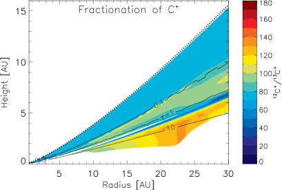
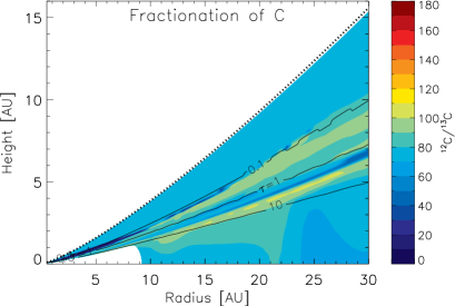
Figure 5: Variation of ¹²C⁺/¹³C⁺ and ¹²C/¹³C throughout the disk.

Fractionation in the top layer of the disk is relatively easy to understand, since all but trace amounts of carbon are to be found in the form of C⁺ (and ¹³C⁺). Thus it follows that the fractionation ratio in this region must reflect the “input” value. For our fiducial model, this input value is 77, and Fig. 5 shows this value in the upper layer of the disk. C⁺ is produced very rapidly, on a timescale of days, mainly by photoionisation of C. This is much faster than a vertical or radial mixing timescale, and thus the fractionation in the upper ionised region is likely to persist as a long-lived feature of the disk. This provides us with a simple way to quantify the carbon fractionation in an observed disk.

The fractionation pattern in the upper, hot layer of the disk shows the need for gas temperature calculations in modelling. Assuming that gas and dust temperatures are identical produces a very uniform disk, with slight increases in fractionation in the transition region, where the difference in self-shielding factors for carbon monoxide is evident. The upper region of the disk has the same degree of fractionation as lower levels, and in general, carbon-bearing species do not reflect the input fractionation ratio. In our model, where the gas temperature is calculated separately from the dust temperature, the activation barrier of reaction (4) becomes negligible at sufficiently high temperatures, such as those found in the disk surface layers. Thus the fractionations in C⁺ and CO are averaged into the input fractionation ratio of 77.

4.2.3 H₂CO, C and the carbon isotope pool

Figure 6: Formaldehyde fractionation shown as the ratio of H${}_{2}^{12}$CO/H${}_{2}^{13}$CO throughout the disk.

The fractionation in H₂CO in interstellar clouds provides one of the upper bounds to the total ¹²C/¹³C ratio (Langer et al. 1984). However, this is not the case in disks, where the fractionation in H₂CO varies from $\sim$60-100 (Fig.6). H₂CO is formed almost exclusively by the reaction between CH₃ and O in the gas phase, and thus the fractionation in H₂CO reflects that in atomic carbon.

The fractionation ratio of atomic carbon in the disk varies from 16–110 (see Fig 5). In general this can be further constrained to $\sim$45–110, with a thin layer 3.3–4.5 $z_{h}$ (0.5$<$R$<$10 AU) where the ratio drops precipitously to $\sim$15. This drop is due to a slight enhancement of the photodissociation rate of ¹³CO over ¹²CO due to the differences in self-shielding, causing the abundance of ¹³C to rise. Atomic carbon is the basis for the formation of many hydrocarbons, and thus species in the carbon isotope pool (e.g., CH, CH₄, etc.) will follow the fractionation in C.

4.2.4 Nitrogen-bearing species

Solid HCN is a major repository of carbon in the cold regions of the disk, storing up to 5% of all available carbon, as well as $\sim$20% of all nitrogen. Desorption of HCN from grain surfaces becomes efficient at a height of $\sim$3.2–3.4$z_{h}$. HCN is then destroyed in the gas phase by photons. What happens to the liberated nitrogen depends on position in the disk. At 3.5$z_{h}$ it is cycled back into HCN through reactions with carbon clusters (C_n). At 3.7$z_{h}$, the availability of oxygen-bearing reactants derived from thermally desorbed H₂O is much greater than at 3.5$z_{h}$, and so N is cycled into NO, and C is cycled into CO through reactions with OH. This causes a slight increase in the abundance of CO, which can be seen in the right panel of Fig. 3.

Solid HCN retains the fractionation ratio of the interstellar cloud model, H¹²CN/H¹³CN = 111. In the gas phase, in intermediate layers of the disk, the fractionation of HCN, HNC and CN is controlled by, and mimics, the fractionation of C.

5 Discussion

5.1 Comparison with previous disk models

The most relevant work on inner disk chemistry is that by Markwick et al. (2002), who study the inner 10 AU of a static disk and assume that the gas temperature is equal to the dust temperature. Their physical model differs greatly from ours, although their chemical network is similar. Markwick et al. (2002) adopt an accretion rate which is a factor of ten larger than ours – this will cause their surface density to be higher, and also their disk to be warmer, in general. The higher surface density means that fewer photons will penetrate the disk, and thus the ionisation profile of the disk is different (their Fig. 3 shows a significantly lower abundance of H⁺ – x(H⁺)$<$10^-12 – than our model – x(H⁺)$<$10^-2). Furthermore, the Markwick et al. (2002) model involves a 1 M_⊙ star, 43% more massive than in our model. A higher stellar mass implies a greater stellar gravity and thus a thinner disk, which receives less stellar UV radiation. Their model also has a temperature inversion, which means that, surprisingly, they find that the majority of species are adsorbed onto dust grains in the surface of the disk at 10 AU. Given this, it is not surprising that the predictions of the two models are very different. Ionisation products such as HCO⁺ are much more abundant in our model (compare Fig. 4 with their Fig. 4), and volatile species are available in the gas phase at different heights and radii due to the difference in the dust temperature profile caused by the different accretion rate.

A more recent model from Agúndez et al. (2008) treats the chemistry in the high density PDR-like regions of protoplanetary disks – the surface of the disk and the inner 3 AU. Agúndez et al. (2008) use a solely gas-phase model to investigate the formation of small species such as HCN, C₂H₂ and CH₄, introducing reactions with significant activation energy barriers ($\sim$1 400 K) which are not included in chemical networks based on interstellar chemistry, such as the UMIST and Ohio State networks. The disk model used by Agúndez et al. (2008) is similar to the one used here, and hence comparison is straightforward. Since they only consider the surface region of the disk, they calculate column densities vertically from a height $z_{\mathrm{in}}$, the height in the disk where the gas is well-shielded to UV radiation and where all the carbon is as CO. In our disk, this corresponds to a height of $\sim$3 $z_{h}$. Agreement is very good for small species such as CO, CO₂, CH₄ and C₂H₂, although the model of Agúndez et al. (2008) is deficient in H₂O, OH, NH₃ and HCN compared to our model. These differences may be explained by different photodissociation rates and activation barriers for these species. For instance, the activation barrier for the reaction H₂ + CN $\longrightarrow$ HCN + H is 1 200 K in Agúndez et al. (2008), but only 820 K in this work, with this value taken from the NIST database.

5.2 Significance for observations

Figure 7: The distribution of HCN and C₂H₂, over-plotted with isotherms (dashed lines) at the rotational temperatures of these molecules in GV Tau (Gibb et al. 2007) – 115 and 170 K, respectively.

Observations of protoplanetary disks at long wavelengths (sub-millimetre and millimetre) are sensitive to the cold gas of the midplane and outer regions (R$>$50–100 AU). Recent observations at infrared wavelengths are sensitive to warmer gas and dust, and thus have been able to probe within a few AU of the star. Future initiatives (e.g., ALMA) which give us high spatial resolution, should enable us to detect material at the radii of Earth-like planet-forming regions in other systems.

Some recent observations have led to derivations of the ¹²C/¹³C ratio in one edge-on (GV Tau (catalog )) and one almost face-on (HL Tau (catalog )) T Tauri disks, similar to the one we model. GV Tau (catalog ) is a binary system in which the T Tauri star has a stellar mass and effective temperature similar to that which we use (White & Hillenbrand 2004). The mass of the disk is estimated to be 0.01 M_⊙ (Hogerheijde et al. 1998). The accretion rate is 20 times greater, 2$\times$10^-7 M_⊙ yr^-1, and the luminosity nearly 2 L_⊙ (White & Hillenbrand 2004). HL Tau (catalog ) has a similar accretion rate and stellar temperature to GV Tau (catalog ), but is nearly twice as massive and slightly less luminous (White & Hillenbrand 2004). The disk around HL Tau (catalog ) extends to at least 200 AU and has a mass of $\sim$0.1 M_⊙ (Gibb et al. 2004). Thus there is a good basis for comparison between our model and these objects.

Through a combination of fundamental and overtone lines of ¹²CO and ¹³CO, Gibb et al. (2007) and Brittain et al. (2005) derived ¹²CO/¹³CO ratios of 54$\pm$15 for GV Tau (catalog ) and 76$\pm$9 for HL Tau (catalog ). These ratios are typical of the transition region (GV Tau (catalog )) and surface regions (HL Tau (catalog )), assuming that these disks have an average ¹²C/¹³C ratio of 77.

Gibb et al. (2007) were able to calculate rotation temperatures for a number of species in GV Tau (catalog ), including HCN (115$\pm$11 K) and C₂H₂ (170$\pm$19 K), as well as ¹²CO (200$\pm$40 K) and ¹³CO (260$\pm$20 K). Using these and other constraints, Gibb et al. (2007) were able to locate the origin of the hydrocarbon absorption to a region above the midplane, possibly the disk atmosphere, within $\sim$10 AU of the central star. These temperatures tally very well with our model: we have plotted the distributions of HCN and C₂H₂ from our model in Fig. 7. The contour lines show isotherms at the rotation temperatures calculated by Gibb et al. (2007). The agreement is very good, especially given the very narrow vertical range in which these two molecules are abundant, due to freezeout in colder layers and either photodestruction or reaction with reactive ions in the layers above. White & Hillenbrand (2004) make an estimate of the luminosity of GV Tau (catalog ) which is larger than that which we use in our model. Taking this into account might move the isotherm closer to the disk midplane, thus improving the agreement with the narrow molecule-rich layers.

Gibb et al. (2007) also derived column densities from their observations through the edge-on disk of GV Tau (catalog ). Brittain et al. (2005) calculated $N$(¹²CO)=7.5 $\times$10¹⁸ cm^-2 and $N$(¹³CO)=9.9 $\times$10¹⁶ cm^-2 from their observations of HL Tau (catalog ), and these column densities correspond to a radius of greater than 35 AU in our model. Derived rotational temperatures of 105 K and 80 K, respectively, indicate that the probed region is an intermediate layer of the disk.

Methane abundances are also constrained by Gibb et al. (2007, 2004), but rotational temperatures are not given. The gas temperature of the methane-rich layer in our disk is $\approx$100 K. In terms of column density, our calculated vertical column densities of $N$(CH₄)=3–21$\times$10¹⁷ cm^-2 at radii in the inner 10 AU of the disk are a factor of 20–300 above the observed upper limits for the GV Tau (catalog ) disk (Gibb et al. 2007). This discrepancy could be down to differences in orientation between GV Tau (catalog ) and our model (column densities of methane and other molecules in our model are calculated vertically, whereas GV Tau (catalog ) is edge-on to the line of sight), or due to uncertainties in the chemistry of methane (perhaps in the accurancy of activation energy barriers in the reactions which lead up to methane formation, see Agúndez et al. 2008). Abundances of methane are also dependent on initial conditions, with methane forming efficiently at the start of the interstellar cloud model on grains, due to high initial abundances of atomic C and H. Calculated column densities are given in Table 3.

Carr & Najita (2008) have probed the inner few AU of the edge-on circumstellar disk of AA Tau (catalog ), a typical classical T Tauri star, with observations from the Spitzer Space Telescope. They report detections of the small molecules CO, C₂H₂, HCN, OH and H₂O, with emission originating from within 2–3 AU of the star. The regions from which this molecular emission arises are hot (525–900 K). CO₂ emission comes from cooler regions (350 K), and thus is assumed to come from larger radii. Our model shows very good correlation between regions of high abundance of these species and gas temperature with the results of Carr & Najita (2008). There is a slight disagreement with C₂H₂, which in our model is found in regions with temperatures of 70–250 K, significantly cooler than the 650 K calculated by Carr & Najita (2008). See Fig. 8, which shows distributions of the molecules detected by Carr & Najita (2008) and isotherms at the designated temperatures attributed to those molecules.

Figure 8: The distribution of CO, CO₂, HCN, C₂H₂, H₂O and OH over-plotted with isotherms (dashed lines) at the rotational temperatures of these molecules in AA Tau (Carr & Najita 2008) – 900, 350, 550, 500, 575 and 525 K, respectively.

Table 3: Selected vertical column densities of molecules in the model disk at 1, 10, 20 and 30 AU

Species		Column at 1 AU		Column at 10 AU		Column at 20 AU		Column at 30 AU
H2		8.3 (24)		1.2 (24)		5.7 (23)		3.7 (23)
He		2.3 (24)		3.3 (23)		1.6 (23)		1.0 (23)
CO		3.7 (20)		5.6 (19)		3.1 (19)		2.4 (19)
CO2		2.4 (19)		3.2 (14)		8.7 (12)		6.3 (12)
CH4		2.1 (18)		2.5 (17)		1.8 (17)		4.3 (18)
C2H2		1.2 (19)		3.2 (15)		7.0 (13)		4.9 (13)
C3H2		6.0 (18)		1.4 (16)		8.7 (15)		7.7 (14)
C3H3		1.6 (18)		3.3 (12)		4.3 (11)		2.9 (12)
C3H4		6.6 (19)		2.5 (16)		9.2 (11)		5.0 (12)
C4H2		2.1 (18)		8.1 (14)		1.1 (15)		5.1 (14)
H2O		2.3 (21)		4.3 (14)		8.1 (13)		7.2 (12)
N2		1.6 (19)		2.1 (17)		1.1 (17)		7.5 (16)
NH3		2.3 (20)		1.2 (15)		3.7 (13)		2.0 (12)
HCN		8.4 (19)		1.6 (15)		2.7 (13)		3.7 (12)
HC3N		7.0 (18)		2.9 (15)		4.2 (13)		9.9 (12)
13CO		7.9 (18)		1.2 (18)		6.3 (17)		4.4 (17)
13CC2H4		1.8 (18)		6.6 (14)		2.8 (10)		1.5 (11)
g–C2H2		1.4 (9)		2.5 (17)		3.2 (18)		1.4 (18)
g–C2H6		1.1 (20)		1.1 (19)		8.4 (17)		2.9 (17)
g–C3H2		2.2 (8)		3.1 (14)		2.4 (18)		2.2 (18)
g–C3H4		8.3 (9)		1.8 (19)		6.2 (18)		1.4 (18)
g–C4H2		1.5 (10)		1.9 (17)		1.6 (18)		1.1 (18)
g–H2O		2.2 (20)		3.5 (20)		1.7 (20)		1.0 (20)
g–NH3		1.9 (12)		3.8 (19)		1.8 (19)		1.2 (19)
g–HCN		1.2 (15)		9.7 (18)		4.6 (18)		3.0 (18)
g–13CCH6		1.9 (18)		2.0 (17)		1.8 (16)		6.1 (15)

Note. — $x$ ($y$) here represents $x\times 10^{y}$ cm^-2. g– before a species denotes that that species is adsorbed onto a grain surface.

5.3 Significance for the Solar System

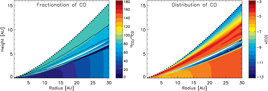
Figure 9: Carbon monoxide fractionation and distribution in the MMSN model. Compare to Fig. 3.

Estimates of the mass of the protosolar disk suggest that it was somewhat more massive than the disk considered in this paper. To make a better comparison with Solar System data we have therefore also considered a model with $\dot{M}$=10^-8 M_⊙ yr^-1 and $\alpha$=0.025, computed for us by Paola D’Alessio. This value of $\alpha$ results in a disk mass similar to the Minimum Mass Solar Nebula (MMSN; Hayashi 1981). All other parameters are the same as the fiducial model, apart from a new scaling for $z_{h}$, $z_{h}$=0.0244R^18/13. We input [¹²C]/[¹³C]=89 to the molecular cloud model to match present Solar System ¹²C/¹³C isotope ratios.

Results from this model differ from the results of our fiducial model in two respects. Since the MMSN model is so much more dense, radial advection times are longer – a parcel of gas will pass from the outer edge of the model at 35 AU into the star in a time of 1.6 Myr, some four times greater than the fiducial model. This gives each parcel a greater processing time at each radius, which leads to:

1) a greater range of degree of fractionation in the disk, such that, for instance, the fractionation in CO decreases from its input value into the disk of 50 to a minimum of 11, compared to 44 and 36, respectively, in the midplane of the fiducial model.

2) a steeper fractionation gradient in the midplane. This increase in range of the fractionation occurs over the same distance in the model, thus the rate of change of fractionation is greater. This is also the case for vertical changes in fractionation, with often large changes in fractionation occurring over small distances ($\sim$1 AU).

These differences can be seen in Fig. 9 for CO.

Measurements of the ¹²C/¹³C ratio in the present day Solar System cluster around the telluric value of 89 (Fig. 10). Although error bars in some cases can be very large, the majority of measurements are consistent with the idea that the bulk of Solar System material comes from a common origin, with an isotope ratio of 89. The most direct comparison we can draw between our MMSN model and present-day fractionation ratios is in the icy matter of comets, which is generally considered to be pristine. Cometary and meteoritic material is thought to be remnant from the very earliest phases of the formation of the Solar System (e.g., Messenger 2000). The degree to which this material has been processed is unknown, although clues can be found in analyses of interplanetary dust particles (IDPs) and carbonaceous chondrites (CCs) on meteorites. IDPs, which become trapped in the Earth’s atmosphere, possibly originate in comets, whilst CCs come from the asteroid belt. Both types of compound may have been subject to heating, mixing and chemical reactions during the history of the solar system, possibly eradicating any chemical “history”. However, the results of carbon fractionation measurements show that in general, all measured comets have a similar ratio (see Fig. 10). Similarly, experiments replicating solar wind or cosmic-ray processing of comet surfaces has shown that these effects do not significantly contribute to carbon isotopic fraction (Lecluse et al. 1998). This is surprising, since ¹²C/¹³C ratios have been derived from both long- and short-period comets, which are thought to have formed in different regions of the protosolar disk.

Carbon fractionation ratios in comets have thus far been determined by observing (one of) three molecules - HCN, CN and C₂ - all members of the carbon isotope pool. CN is most likely a photodissociation product of HCN in cometary comae, although other parents may exist (Arpigny et al. 2003). In our MMSN disk model CN and C₂ ices are of very low abundance, which makes it difficult to give a ¹²C/¹³C ratio with a high degree of confidence. However, HCN ice is more plentiful, and has a ¹²C/¹³C ratio of 126–129 in the midplane region of the disk model. This ratio is inherited from the molecular cloud. It matches very well with observations of Comet Hale Bopp, a long-period comet: H¹²CN/H¹³CN = 110$\pm$12 (Jewitt et al. 1997; Ziurys et al. 1999), but not with Comet Hyakutake: H¹²CN/H¹³CN = 34$\pm$12 (Lis et al. 1997). To our knowledge these are the only three determinations of the H¹²CN/H¹³CN in comets. In the disk model, CN generally has a similar fractionation ratio to HCN. However, fractionation ratios derived from observations of CN in comets are somewhat different to HCN, in the region 65-115, with an average of $\sim$90. This may be another indication of the alternative parentage of the CN molecule, or perhaps that there are some photo-fractionation effects in the photodissociation of HCN.

Figure 10: Measurements of the ¹²C/¹³C ratio in various objects of the Solar System. Filled circles indicate measurements of planets or the Sun and empty circles indicate measurements of planetary moons. Triangles indicate bulk isotope measurements of the ¹²C/¹³C ratio in meteorites, and have been placed at the radius of the asteroid belt. Comets, indicated by filled stars, have been placed outside of the radius of Neptune, for illustration, and similarly, IDPs (filled squares) have been placed at cometary radii to indicate their likely origin in comets. Please contact the author for a full list of references for the data in this plot.

What conclusions, then, can be drawn from this work given that our standard model of fractionation in a protoplanetary disk produces a very “stratified” result, where fractionation differs from region to region in the disk, and also from species to species? One possibility is that the protosolar disk was heated to some sufficiently high temperature for chemical exchange reactions to be ineffectual. This may have had the effect of “resetting” the carbon isotope ratios, similar to the process which occurred later in the formation of individual planets and the Sun. However, cooling from this state would have to have been relatively fast, faster than the chemical timescales for fractionation.

A slightly different possibility relies on mixing material up to the surface layers of the disk, heating and photodestroying it, leading to a reset of the the carbon isotope ratio. For the processed material to be mixed down to the planetary accretion zones at the midplane of the disk would require vertical mixing timescales to be fast in relation to both the chemical timescales and accretion timescales. Given the high densities in the MMSN model, this seems unlikely since collision times and chemical reaction times will be short.

A third consideration is that of nebular shocks, which may have transiently heated material in the inner nebula (Desch & Connolly 2002; Kress et al. 2002). Processed material could then have rapidly cooled and frozen out onto grain surfaces within chemical fractionation timescales, thus locking in the carbon isotope ratio of the hotter gas. However, the entire nebula would have had to have passed through such a shock to produce such a uniform carbon isotope ratio.

So we conclude that whatever the mechanism which homogenised carbon isotope fractionation ratios in the Solar System (and these mechanisms bear future investigation), it occurred before comets and planets formed, yet after the initial collapse of the solar nebula’s parent molecular cloud.

6 Conclusions

We have shown by means of a chemical model of a protoplanetary disk that the fractionation ratio of carbon, ¹²C/¹³C, varies according to position in the disk. The fractionation ratio is governed by temperature, which affects the rate and direction of chemical exchange reactions, and incident UV radiation, which affects self-shielding molecules such as CO. This produces a picture of the fractionation in a disk which is stratified. Certainly in the upper region of the disk, fractionation timescales are faster than mixing timescales, meaning that this stratified picture should persist if mixing were to be considered in the model. We also considered a Minimum Mass Solar Nebula model in which the chemistry in our inflowing gas packets has longer to evolve. Extremely good agreement was seen between observations of Solar System comets and the fractionation ratio in ices in the midplane of the disk model. In general, our chemical model has excellent agreement with recent observations of T Tauri disks, both in terms of chemical abundance and location in the disk.

Appendix A Gas heating and cooling mechanisms

A.1 Heating

Photoelectric heating.

Photoelectrons are emitted from dust grains when UV photons impinge upon the grain. The energy of these emitted particles depends on the energy of the incident photon and on the emitting grain potential. The gas heating rate due to photoelectrons is approximated by Bakes & Tielens (1994), and is implemented as follows (Kamp & van Zadelhoff 2001).

For the purposes of the thermal balance, we assume that there are two populations of dust grain within the disk – one consisting of silicate particles and the other consisting of a mixture of small graphitic and PAH grains. The silicate grains are assumed to have a radius, $a=0.1$ $\mu$m, and a UV cross section per H nucleus ($\sigma_{\mathrm{UV}}$) of $5.856\times 10^{-22}$ cm²/H atom (Kamp & Dullemond 2004). The small graphite grains are assumed to have a size distribution ranging from 3–100Å(Bakes & Tielens 1994). Larger grains do not contribute to the disk heating.

Thus the photoelectric heating rate, $\Gamma_{\mathrm{PE}}$, is given by:

$$\Gamma_{\mathrm{PE}}=b\epsilon\chi n_{0}\quad\mathrm{erg\,cm^{-3}\,s^{-1}}$$ (A1)

(Bakes & Tielens 1994) where $\epsilon$ is an efficiency factor depending on the material of the grain, $\chi$ is the photon flux measured in units of the Habing (1968) field between 912-1110 Å attenuated by dust and $n_{0}$ is the total number density of hydrogen nuclei, $n_{0}$=2$n_{\mathrm{H_{2}}}$+$n_{\mathrm{H}}$. $b$ is a constant and is equal to $1\times 10^{-24}$ for graphite/PAH grains and $2.5\times 10^{-4}\sigma_{\mathrm{UV}}$ for silicate grains, with $\sigma_{\mathrm{UV}}=Q_{\mathrm{abs}}\pi a^{2}n_{\mathrm{d}}$, where $Q_{\mathrm{abs}}$ is a UV absorption efficiency and $n_{\mathrm{d}}$ is the number density of dust grains.

The photoelectric efficiencies and yields depend on material. Following Kamp & van Zadelhoff (2001), we define a grain charge parameter, $x\equiv\chi T^{0.5}/n_{\mathrm{e}}$, with $n_{\mathrm{e}}$ the electron density. Thus,

$$\epsilon_{\mathrm{sil}} = \frac{6\times 10^{-2}}{1+1.8\times 10^{-3}x^{0.91}}+\frac{1.6\times 10^{-5}y_{\mathrm{sil}}T^{1.2}}{1+1\times 10^{-2}x}$$ (A2)

$$\epsilon_{\mathrm{PAH}} = \frac{0.0487}{1+4.0\times 10^{-3}x^{0.73}}+\frac{5.8\times 10^{-5}T^{0.7}}{1+2\times 10^{-4}x}.$$ (A3)

(Kamp & van Zadelhoff 2001). The yields for silicate material ($y_{\mathrm{sil}}$) are:

$$y_{\mathrm{sil}}=\left\{\begin{array}[]{cl}0.70&\mathrm{for~{}}x\leq 10^{-4}\\ 0.36&\mathrm{for~{}}10^{-4}<x\leq 1\\ 0.15&\mathrm{for~{}}x>1\end{array}\right.$$ (A7)

Collisional de-excitation of H₂.

H₂ molecules in excited rovibrational levels (due to Lyman-Werner band absorptions, for example) can decay to less energetic levels following collisions, thereby heating the gas in the process. This complex situation was simplified by Tielens & Hollenbach (1985) by considering a single excited pseudovibrational level of H₂. They derived the following heating rate:

$$\Gamma_{\mathrm{CDx}}=(n_{\mathrm{H}}\gamma_{\mathrm{*0}}^{\mathrm{H}}+n_{\mathrm{H_{2}}}\gamma_{\mathrm{*0}}^{\mathrm{H_{2}}})n_{\mathrm{H_{2}^{*}}}E_{*}\quad\mathrm{erg\,cm^{-3}\,s^{-1}},$$ (A8)

where $n_{\mathrm{H}}$ is the number density of atomic hydrogen, $n_{\mathrm{H_{2}}}$ is the number density of molecular hydrogen, $n_{\mathrm{H_{2}^{*}}}$ is the number density of vibrationally excited H₂ (presumed to be a fixed proportion of H₂, $n_{\mathrm{H_{2}^{*}}}$=$10^{-5}n_{\mathrm{H_{2}}}$) and $E_{*}$ is the effective energy of the pseudolevel (taken to be $4.166\times 10^{-12}$ ergs, London 1978). $\gamma_{\mathrm{*0}}^{\mathrm{H}}$ and $\gamma_{\mathrm{*0}}^{\mathrm{H_{2}}}$ are the collisional de-excitation rate coefficients from the excited $v$=6 level to the $v$=0 level. Since these transitions tend to occur in steps of $\Delta v$=1, $\gamma_{\mathrm{*0}}^{\mathrm{H}}$ and $\gamma_{\mathrm{*0}}^{\mathrm{H_{2}}}$ are assumed to equal to one sixth of the $v$=1-0 rate coefficients (Tielens & Hollenbach 1985). Thus $\gamma_{\mathrm{*0}}^{\mathrm{H}}=1.67\times 10^{-13}\sqrt{T}\exp(-1\,000\,\mathrm{K}/T)$ cm³ s^-1 and $\gamma_{\mathrm{*0}}^{\mathrm{H_{2}}}=2.33\times 10^{-13}\sqrt{T}\exp(-18\,100\,\mathrm{K}/[T+1\,200\,\mathrm{K}])$ cm³ s^-1.

Photodissociation of H₂.

Whilst 90% of Lyman-Werner band excitation results in collisional de-excitation, the remaining 10% results in radiative dissociation to a pair a hydrogen atoms, each carrying approximately 0.4 eV of kinetic energy (Stephens & Dalgarno 1973). Hence the heating rate due to photodissociation of H₂ can be approximated:

$$\Gamma_{\mathrm{Phd}}=5.55\times 10^{-13}\chi\Gamma_{\mathrm{H_{2}}}^{\prime}n_{\mathrm{H_{2}}}\quad\mathrm{erg\,cm^{-3}\,s^{-1}}$$ (A9)

(Tielens & Hollenbach 1985). Here $\Gamma_{\mathrm{H_{2}}}^{\prime}$ is the photodissociation rate of H₂, taking self-shielding into account (see Sect. 3.1.2).

H₂ formation.

The formation and release of a hydrogen molecule from the surface of a dust grain contributes 4.48 eV of binding energy to the thermal balance. Since it is unclear how much of that energy is transferred into rotation, vibration and translation, we follow the approach of Black & Dalgarno (1976) (and also Kamp & van Zadelhoff 2001) by assuming that one third goes into each motion. This results in a heating rate due to H₂ formation:

$$\Gamma_{\mathrm{Form}}=2.39\times 10^{-12}R_{\mathrm{form}}\quad\mathrm{erg\,cm^{-3}\,s^{-1}}.$$ (A10)

$R_{\mathrm{form}}$ is the formation rate of H₂ taken from Cazaux & Tielens (2002b), which incorporates revised H₂ formation efficiencies ($\epsilon_{\mathrm{H_{2}}}$) at high temperatures, viz.

$$R_{\mathrm{form}} = 0.5n(\mathrm{H})v_{\mathrm{H}}n_{\mathrm{d}}\sigma_{\mathrm{d}}\epsilon_{\mathrm{H_{2}}}S_{\mathrm{H}}\quad\mathrm{cm^{-3}\,s^{-1}}$$ (A11)

$$\epsilon_{\mathrm{H_{2}}} = \left(1+\frac{\mu F}{2\beta_{\mathrm{H_{2}}}}+\frac{\beta_{\mathrm{H_{p}}}}{\alpha_{\mathrm{pc}}}\right)^{-1}\xi$$ (A12)

$$\xi = \left[1+\frac{\nu_{\mathrm{H_{c}}}}{2F}\exp\left(-\frac{1.5E_{\mathrm{H_{c}}}}{kT}\right)\left(1+\sqrt{\frac{E_{\mathrm{H_{c}}}-E_{\mathrm{s}}}{E_{\mathrm{H_{p}}}-E_{\mathrm{s}}}}\right)^{2}\right]^{-1}.$$ (A13)

$v_{\mathrm{H}}$ is the velocity of a hydrogen atom and $\sigma_{\mathrm{d}}$ is the geometric cross section of a grain. $n_{\mathrm{d}}$ is usually assumed to be $\approx$10${}^{-12}n_{0}$, but can be calculated from the gas density:

$$n_{\mathrm{d}}=\delta_{\mathrm{dg}}n_{0}\mu m_{\mathrm{H}}\left(\frac{4\pi a^{3}\rho_{\mathrm{d}}}{3}\right)^{-1}\quad\mathrm{cm}^{-3}.$$ (A14)

We adopt a standard dust-to-gas mass ratio ($\delta_{\mathrm{dg}}$) of 0.01, a grain density ($\rho_{\mathrm{d}}$) of 2.5 g cm^-3 and a grain size ($a$) of 0.1$\mu$m. $\mu$ is the reduced mass of the gas (taken to be 2.4) and $m_{\mathrm{H}}$ the mass of an H atom. $S_{\mathrm{H}}$ in Eq. A11 is the sticking coefficient of hydrogen and is assumed to be 0.4, in line with Cazaux & Tielens (2004). The reader is referred to Cazaux & Tielens (2002a, b) for an explanation of the other terms. In the calculation of $\epsilon_{\mathrm{H_{2}}}$ we assume $F$=10^-15 (Kamp, priv. comm.), where $F$ is the accretion rate of H₂ in units of monolayers per second. In the calculation of $\xi$, we assume that when a grain is completely covered with a monolayer of ice no chemisorption of H atoms can occur, but physisorption can. Thus in Eq. A13, $E_{\mathrm{H_{c}}}$=$E_{\mathrm{H_{p}}}$=600 K, rather than $E_{\mathrm{H_{c}}}$=10 000 K in the chemisorption case.

C ionisation.

Neutral carbon can be readily photoionised in protoplanetary disks, with the release of approximately 1 eV of energy per ionisation (Black 1987). The heating rate due to this process depends on the attenuation by dust absorption (Black & Dalgarno 1977), attenuation by self-absorption of C (Werner 1970) and also attenuation by the H₂ column (de Jong et al. 1980) (the first, second and third exponential terms, respectively).

$$\Gamma_{\mathrm{CIon}}=2.2\times 10^{-22}n(\mathrm{C})\chi_{0}\frac{\exp(-2.4A_{\mathrm{V}}-\tau_{\mathrm{C}}-\tau_{\mathrm{H_{2}}}v_{2}/\pi v_{1}^{2})}{1+\tau_{\mathrm{H_{2}}}v_{2}/\pi v_{1}^{2}}\quad\mathrm{erg\,cm^{-3}\,s^{-1}}$$ (A15)

(Tielens & Hollenbach 1985). The various parameters are given by:

$$\tau_{\mathrm{C}}=10^{-17}N(\mathrm{C}), \tau_{\mathrm{H_{2}}}=1.2\times 10^{-14}N(\mathrm{H_{2}})\delta v^{-1},$$

$$\quad v_{2}=9.2\times 10^{-3}\delta v^{-1}, v_{1}=5\times 10^{2}\delta v^{-1}.$$ (A16)

$\chi_{0}$ is the unattenuated photon flux incident on the surface of the disk, $N(\mathrm{H_{2}})$ and $N(\mathrm{C})$ are the column densities of molecular hydrogen and atomic carbon, respectively. $\delta v$ is the line broadening, taken to be equal to the sound speed.

Cosmic ray heating.

Cosmic rays will penetrate the disk up until a certain column density of matter (150 g cm^-2; Umebayashi & Nakano 1981), and contribute to the thermal balance via the energy released in the formation and subsequent electronic recombination of H${}_{3}^{+}$. This process yields some 7 eV per ionisation (Glassgold & Langer 1973). The heating rate is given by:

$$\Gamma_{\mathrm{C-ray}}=(1+n_{\mathrm{He}}/n_{0})\zeta_{\mathrm{H}}n_{0}(1.28\times 10^{-11}+2.44\times 10^{-11}(n_{\mathrm{H_{2}}}/n_{0}))\quad\mathrm{erg\,cm^{-3}\,s^{-1}}$$ (A17)

(Clavel et al. 1978), where $n_{\mathrm{He}}$ is the number density of helium. For $\zeta_{\mathrm{H}}$, the cosmic ray ionisation rate of hydrogen, we use the value of 5.98$\times$10^-18 s^-1 (Woodall et al. 2007).

X-ray heating.

To calculate the heating effect due to X-rays we use the prescription of Gorti & Hollenbach (2004) for an X-ray energy spectrum of 0.5-10 keV:

$$\Gamma_{\mathrm{X-ray}}=\int_{0.5}^{10}F(E)\exp(-N_{0}\sigma_{\mathrm{X}}(E))\sigma_{\mathrm{X}}(E)n_{0}f_{\mathrm{heat}}dE\quad\mathrm{erg\,cm^{-3}\,s^{-1}}.$$ (A18)

$F(E)$ is the X-ray photon flux at a radius R: $L(E)$/$4\pi R^{2}$, where $L(E)$ is the stellar luminosity as a function of emitted energy (in keV). Gorti & Hollenbach (2004) fit a broken power law to the X-ray spectrum of a weak-line T Tauri star presented in Feigelson & Montmerle (1999), resulting in:

$$L(E)=\left\{\begin{array}[]{cl}1.2L_{\mathrm{X}}E^{-1.75}&\mathrm{for~{}}E>2\,\mathrm{keV},\\ 0.18L_{\mathrm{X}}E&\mathrm{for~{}}E<2\,\mathrm{keV}.\end{array}\right.$$ (A21)

$L_{\mathrm{X}}$ is the X-ray luminosity of the central star in ergs s^-1, which is in general 10^-3–$10^{-4}\,L_{\star}$ (Feigelson & Montmerle 1999). We use $L_{\mathrm{X}}$=$10^{-4}\,L_{\star}$, and use the fit in Eq. A21, since the X-ray spectrum of a classical T Tauri star resembles that of a weak-line T Tauri star quite closely (Feigelson & Montmerle 1999). In Eq. A18, $N_{0}$ is the hydrogen nucleus column density of gas towards the central star, and $\sigma_{\mathrm{X}}(E)$ is the total X-ray photoabsorption cross-section per H nucleus:

$$\sigma_{\mathrm{X}}(E)=2.27\times 10^{-22}(E/1\,\mathrm{keV})^{-2.485}\quad\mathrm{cm^{2}/H~{}nucleus},$$ (A22)

(Wilms et al. 2000). $f_{\mathrm{heat}}$ is the fraction of absorbed energy which heats the gas, equal to 0.1 for atomic gas and 0.4 for molecular gas (Maloney et al. 1996).

There is also a secondary X-ray heating effect since the recombination of H⁺ after ionisation results in a substantial population of H atoms in an excited state, which decay collisionally. Thus the primary rate (Eq. A18) is augmented by an additional:

$$\Gamma_{\mathrm{X-ray}}^{\prime}=2.22\zeta_{\mathrm{X}}^{\mathrm{H}}n_{\mathrm{H}}E_{21}\quad\mathrm{erg\,cm^{-3}\,s^{-1}}$$ (A23)

(Shang et al. 2002). $\zeta_{\mathrm{X}}^{\mathrm{H}}$ is the X-ray ionisation rate of atomic hydrogen and $E_{21}$ the energy gap between the $n$=2 and $n$=1 excited levels of a hydrogen atom (10.19 eV). $\zeta_{\mathrm{X}}^{\mathrm{H}}$ is calculated according to the process described in Sect. 3.2.

A.2 Cooling

The gas in a PPD is cooled by the line emission of atomic and molecular species, and also, when the gas temperature is greater than the dust temperature, by collisions between gas and dust.

For the emission lines, we generally make use of the escape probability factor, $\beta(\tau)$. This factor takes into account the fact that atomic and molecular lines can have a much higher optical depth than that of the dust continuum. The escape probability factor, then, is the probability that a photon from a particular line with an optical depth, $\tau$, will escape from the disk. The maximum probability is 0.5, since we assume that any photons emitted in the negative $z$ direction will be absorbed in the disk.

Tielens & Hollenbach (1985) show that the optical depth in the vertical direction $z$ is:

$$\tau(z)=A_{ul}\frac{c^{3}}{8\pi\nu^{3}(\delta v)}\int_{0}^{z}n_{u}(z^{\prime})\left(\frac{n_{l}(z^{\prime})g_{u}}{n_{u}(z^{\prime})g_{l}}-1\right)dz^{\prime},$$ (A24)

where $z$=0 is the surface of the disk, contrary to our usual notation. In Eq. A24, $A_{ul}$ is the Einstein transition probability from level $u$ to level $l$, $\nu$ is the line frequency, $\delta v$ is the line broadening (assumed to be equal to the sound speed, $c_{\mathrm{S}}$), $n_{u}$ and $n_{l}$ are the level populations of levels $u$ and $l$, and $g_{u}$ and $g_{l}$ are the corresponding statistical weights. Ideally, the optical depth would be calculated by solving the level population equations in non-local thermal equilibrium (non-LTE). However, this is computationally expensive, and we have had to make assumptions in order to simplify the calculation. Hence we assume a plane-parallel slab, with uniform temperature and density. Level populations are in LTE. The optical depth then becomes:

$$\tau(z)=\frac{A_{ul}c^{3}n_{1}z}{8\pi\nu^{3}(\delta v)}\left[\exp\left(\frac{h\nu_{ul}}{kT}\right)-1\right],$$ (A25)

(Tielens & Hollenbach 1985).

The escape probability formalism is defined by de Jong et al. (1980):

$$\beta(\tau)=\left\{\begin{array}[]{cl}\frac{1-\exp(-2.34\tau)}{4.68\tau}&\mathrm{for~{}}\tau<7,\\ \left[4\tau\left(\ln\frac{\tau}{\sqrt{\pi}}\right)^{0.5}\right]^{-1}&\mathrm{for~{}}\tau\geq 7.\end{array}\right.$$ (A28)

Atomic line cooling.

To calculate electronic level populations, we solve the statistical equilibrium equations for a three-level system:

$$n_{i}\sum_{j\neq i}R_{ij}=\sum_{j\neq i}n_{j}R_{ji}\qquad\mathrm{and}\qquad n_{\mathrm{X}}=\sum_{j=0}^{2}n_{j},$$ (A29)

where $n_{\mathrm{X}}$ is the number density of species X and

$$R_{ij}=\left\{\begin{array}[]{cl}A_{ij}\beta(\tau_{ij})(1+Q_{ij})+C_{ij}&\mathrm{for~{}}i>j,\\ (g_{j}/g_{i})A_{ji}\beta(\tau_{ji})Q_{ji}+C_{ji},&\mathrm{for~{}}i<j,\end{array}\right.$$ (A32)

with

$$Q_{ij}=Q_{ji} = \frac{c^{2}}{2h\nu_{ij}^{3}}P(\nu_{ij})$$ (A33)

$$P(\nu_{ij})=B(\nu_{ij},2.7\,\mathrm{K}) + B(\nu_{ij},T_{\mathrm{d}})\tau_{d}(\nu_{ij}).$$ (A34)

where $C_{ij}$ is the collisional rate from level $i$ to level $j$ and $P(\nu_{ij})$ denotes the background radiation due to 1) the 2.7 K microwave background, and 2) the infrared emission of dust, expressed in terms of Planck blackbody functions, with $T_{\mathrm{d}}$ the dust temperature and $\tau_{d}(\nu_{ij})$=0.001 (Hollenbach et al. 1991). Assuming that the local radiation field in the disk can be represented by the sum of these two blackbodies is a simplification: it ignores the significant effect of stellar radiation in the disk surface and neglects the fact that in the disk midplane the local radiation is optically thick, and thus not proportional to $\tau_{d}(\nu_{ij})$. This assumption will affect the cooling rate and thus the gas temperature (see, for example Kamp & van Zadelhoff 2001).

We consider the fine-structure lines of [Oi], [Ci] and [Cii], in the manner described above in Eqs. A25–A33, calculating the statistical equilibrium in detail, since some regions of the disk are below the critical density required for LTE to be a reasonable assumption.

The lowest three fine structure lines for [Oi] are at 63.2, 145.6 and 44.0 $\mu$m. Line data is taken from Table 1 of Kamp & van Zadelhoff (2001), who take into account collisions with H₂, H and electrons. The cooling rate over all three lines is:

$$\Lambda_{\mathrm{O}\textsc{i}}=\sum_{k}\beta(\tau_{ul})h\nu_{ul}[n_{u}(\mathrm{O})(A_{ul}+B_{ul}P(\nu_{ul}))-n_{l}(\mathrm{O})B_{lu}P(\nu_{ul})]\quad\mathrm{erg\,cm^{-3}\,s^{-1}}.$$ (A35)

(Kamp & van Zadelhoff 2001). $h$ is the Planck constant, $\nu_{ul}$ the frequency of the fine-structure line, $n_{u}$(O) and $n_{l}$(O) are the number densities of oxygen in the upper and lower levels of the transition, respectively, and $A_{ul}$, $B_{ul}$ and $B_{lu}$ are the Einstein coefficients for the transition.

A similar approach is taken for [Ci], although the critical density for the three [Ci] cooling lines at 609.2, 229.9 and 369.0 $\mu$m is much lower, and LTE can be assumed. Again, atomic data is taken from Kamp & van Zadelhoff (2001). The cooling rate is simply:

$$\Lambda_{\mathrm{C}\textsc{i}}=h[A_{10}\beta(\tau_{10})\nu_{10}n_{1}(\mathrm{C})+A_{20}\beta(\tau_{20})\nu_{20}n_{2}(\mathrm{C})+A_{21}\beta(\tau_{21})\nu_{21}n_{2}(\mathrm{C})]\quad\mathrm{erg\,cm^{-3}\,s^{-1}},$$ (A36)

(Kamp & van Zadelhoff 2001).

We also consider the [Cii] line at 157.7 $\mu$m, again assuming LTE since the density in the disk is always above the critical density for this transition. The cooling rate is:

$$\Lambda_{\mathrm{C}\textsc{ii}}=A_{10}\beta(\tau_{10})h\nu_{10}n_{1}(\mathrm{C^{+}})\quad\mathrm{erg\,cm^{-3}\,s^{-1}},$$ (A37)

with atomic data from Kamp & van Zadelhoff (2001).

Molecular line cooling.

H₂ rotational/vibrational and CO rotational line cooling are the main molecular cooling lines in the disk, although we have also taken into account cooling from CH molecules.

The H₂ cooling function for the lowest 51 rovibrational energy levels has been derived by Le Bourlot et al. (1999), taking into account collisions with H, He and H₂, but not including pumping by UV and X-ray radiation which will affect the H₂ population in high energy levels. It is only strictly valid between temperatures of 10²–10⁴ K and densities of 1–10⁸ cm^-3. H₂ cooling is negligible at densities less than 10⁶ cm^-3 (Hollenbach & McKee 1979) and at temperatures less than 100 K, and we persist in using the function at the high densities which can be found in the disk. We adopt an ortho-to-para ratio of 1.

26 rotational lines of CO are considered in calculating the cooling rate due to CO emission:

$$\Lambda_{\mathrm{CO}}=\beta(\tau_{\mathrm{CO}})\sum_{i=1}^{25}h\nu_{ij}[n_{i}(\mathrm{CO})(A_{ij}+B_{ij}P(\nu_{ij}))-n_{j}(\mathrm{CO})B_{ji}P(\nu_{ij})]\quad\mathrm{erg\,cm^{-3}\,s^{-1}}.$$ (A38)

Collisional rate coefficients are from Schinke et al. (1985), and other molecular data from Kamp & van Zadelhoff (2001). The optical depth of CO lines is calculated using Eq. A24.

The emission lines of CH radicals have a minimal effect on the thermal balance in the inner disk, but can provide cooling in regions where CH is particularly abundant. We use the cooling rate of Kamp & van Zadelhoff (2001),

$$\Lambda_{\mathrm{CH}}=\beta(\tau_{\mathrm{CH}})n_{0}n_{\mathrm{CH}}L_{\mathrm{rot}}\quad\mathrm{erg\,cm^{-3}\,s^{-1}},$$ (A39)

where the line cooling coefficient, $L_{\mathrm{rot}}$, is derived by Hollenbach & McKee (1979):

$$L_{\mathrm{rot}}=\left\{\begin{array}[]{cl}\frac{4(kT)^{2}A_{0}}{n_{0}E_{0}(1+(n_{\mathrm{cr}}/n_{0})+1.5\sqrt{n_{\mathrm{cr}}/n_{0}})}&\mathrm{erg\,cm^{3}\,s^{-1}~{}for~{}}n_{0}\gg n_{\mathrm{cr}},\\ \frac{kT(1-(n_{\mathrm{H_{2}}}/n_{0}))\sigma_{\mathrm{tot}}v_{\mathrm{T}}}{(1+(n_{0}/n_{\mathrm{cr}})+1.5\sqrt{n_{0}/n_{\mathrm{cr}}})}&\mathrm{erg\,cm^{3}\,s^{-1}~{}for~{}}n_{0}\ll n_{\mathrm{cr}},\end{array}\right.$$ (A42)

and $\beta(\tau_{\mathrm{CH}})$=1, which overestimates the cooling rate. The critical density for CH, $n_{\mathrm{cr}}$, is 6.6$\times$10${}^{9}\sqrt{(T/1\,000\,\mathrm{K})}$ cm^-3, and $A_{0}$ and $E_{0}$ are 7.7$\times$10^-3 s^-1 and 2.76$\times$10^-15 erg respectively. The total inelastic cross-section of CH, $\sigma_{\mathrm{tot}}$, is taken to be 1$\times$10^-15 cm² (Hollenbach & McKee 1979). $v_{\mathrm{T}}$ is the thermal velocity of the colliding hydrogen atoms.

Cooling at high temperatures.

At high temperatures (more than several hundred degrees Kelvin) Ly$\alpha$ and the line emission from the metastable ¹D–³P transition of atomic oxygen at 6300 Å efficiently cool the gas. Cooling rates for both these processes are given by Sternberg & Dalgarno (1989):

$$\Lambda_{\mathrm{Ly\alpha}} = 7.3\times 10^{-19}\beta(\tau_{\mathrm{Ly\alpha}})n_{\mathrm{e}}n_{\mathrm{H}}\exp(-118\,400\,\mathrm{K}/T)\quad\mathrm{erg\,cm^{-3}\,s^{-1}},$$ (A43)

$$\Lambda_{\mathrm{O6300}} = 1.8\times 10^{-24}\beta(\tau_{\mathrm{O6300}})n_{\mathrm{O}}\exp(-22\,800\,\mathrm{K}/T)\times$$ (A44)

$$\qquad\qquad\left[n_{\mathrm{H}}+n_{\mathrm{H_{2}}}+\frac{410n_{\mathrm{e}}}{(9T^{1/2}+6.3\times 10^{-8}n_{\mathrm{e}}T)}\right]\quad\mathrm{erg\,cm^{-3}\,s^{-1}},$$

with $n_{\mathrm{O}}$ the number density of oxygen. The third term in the brackets in Eq. A44 takes into account excitation of the oxygen atoms by impacting electrons, as described in Draine et al. (1983). $\beta(\tau_{\mathrm{Ly\alpha}})$=$\beta(\tau_{\mathrm{O6300}})$=1.

Gas-grain collisions.

Collisions between dust grains and atoms and molecules will generally act as an energy transfer mechanism, and will cool the gas if the gas temperature is larger than the dust temperature, which is generally the case in the regions under consideration. The heating rate due to these collisions is:

$$\Lambda_{\mathrm{G-G}}=4.0\times 10^{-12}(\pi a^{2})n_{0}n_{\mathrm{d}}\alpha_{\mathrm{T}}\sqrt{T}(T-T_{\mathrm{d}})\quad\mathrm{erg\,cm^{-3}\,s^{-1}},$$ (A45)

where $a$=0.1 $\mu$m, the thermal accommodation coefficient, $\alpha_{\mathrm{T}}$=0.3 (Burke & Hollenbach 1983) and $n_{\mathrm{d}}$ is defined previously (Eq. A14).

References

- Agúndez et al. (2008) Agúndez, M., Cernicharo, J., & Goicoechea, J. R. 2008, A&A, 483, 831
- Aikawa & Nomura (2006) Aikawa, Y., & Nomura, H. 2006, ApJ, 642, 1152
- Aikawa & Herbst (2001) Aikawa, Y., & Herbst, E. 2001, A&A, 371, 1107
- Aikawa & Herbst (1999) Aikawa, Y. & Herbst, E. 1999, A&A, 351, 233
- Aikawa et al. (1999) Aikawa, Y., Umebayashi, T., Nakano, T., & Miyama, S. M. 1999, ApJ, 519, 705
- Anders & Grevesse (1989) Anders, E. & Grevesse, N. 1989, Geochim. Cosmochim. Acta, 53, 197
- Andrews & Williams (2007) Andrews, S. M. & Williams, J. P. 2007, ApJ, 659, 705
- Arpigny et al. (2003) Arpigny, C., Jehin, E., Manfroid, J., Hutsemékers, D., Schulz, R., Stüwe, J. A., Zucconi, J.-M., & Ilyin, I. 2003, Science, 301, 1522
- Artymowicz & Clampin (1997) Artymowicz, P. & Clampin, M. 1997, ApJ, 490, 863
- Ayres et al. (2006) Ayres, T. R., Plymate, C., & Keller, C. U. 2006, ApJS, 165, 618
- Bakes & Tielens (1994) Bakes, E. L. O. & Tielens, A. G. G. M. 1994, ApJ, 427, 822
- Bensch et al. (2001) Bensch, F., Pak, I., Wouterloot, J. G. A., Klapper, G., & Winnewisser, G. 2001, ApJ, 562, L185
- Bergin et al. (2003) Bergin, E., Calvet, N., D’Alessio, P., & Herczeg, G. J. 2003, ApJ, 591, L159
- Bisschop et al. (2006) Bisschop, S. E., Fraser, H. J., Öberg, K. I., van Dishoeck, E. F., & Schlemmer, S. 2006, A&A, 449, 1297
- Black (1987) Black, J. H. 1987, in Astrophysics and Space Science Library, Vol. 134, Interstellar Processes, ed. D. J. Hollenbach & H. A. Thronson, Jr., 731–744
- Black & Dalgarno (1976) Black, J. H. & Dalgarno, A. 1976, ApJ, 203, 132
- Black & Dalgarno (1977) —. 1977, ApJS, 34, 405
- Blake & Boogert (2004) Blake, G. A. & Boogert, A. C. A. 2004, ApJ, 606, L73
- Boogert et al. (2000a) Boogert, A. C. A., Tielens, A. G. G. M., Ceccarelli, C., Boonman, A. M. S., van Dishoeck, E. F., Keane, J. V., Whittet, D. C. B., & de Graauw, T. 2000, A&A, 360, 683
- Boogert et al. (2000b) Boogert, A. C. A., et al. 2000, A&A, 353, 349
- Boogert et al. (2002) Boogert, A. C. A., Blake, G. A., & Tielens, A. G. G. M. 2002, ApJ, 577, 271
- Brittain et al. (2005) Brittain, S. D., Rettig, T. W., Simon, T., & Kulesa, C. 2005, ApJ, 626, 283
- Brittain et al. (2003) Brittain, S. D., Rettig, T. W., Simon, T., Kulesa, C., DiSanti, M. A., & Dello Russo, N. 2003, ApJ, 588, 535
- Burke & Hollenbach (1983) Burke, J. R. & Hollenbach, D. J. 1983, ApJ, 265, 223
- Carr & Najita (2008) Carr, J. S., & Najita, J. R. 2008, Science, 319, 1504
- Carr et al. (2004) Carr, J. S., Tokunaga, A. T., & Najita, J. 2004, ApJ, 603, 213
- Casassus et al. (2005) Casassus, S., Stahl, O., & Wilson, T. L. 2005, A&A, 441, 181
- Cazaux & Tielens (2002a) Cazaux, S. & Tielens, A. G. G. M. 2002a, ApJ, 577, L127