Searching bifurcations in high-dimensional parameter space via a feedback loop breaking approach

Abstract

Bifurcations leading to complex dynamical behaviour of non-linear systems are often encountered when the characteristics of feedback circuits in the system are varied. In systems with many unknown or varying parameters, it is an interesting, but difficult problem to find parameter values for which specific bifurcations occur. In this paper, we develop a loop breaking approach to evaluate the influence of parameter values on feedback circuit characteristics. This approach allows a theoretical classification of feedback circuit characteristics related to possible bifurcations in the system. Based on the theoretical results, a numerical algorithm for bifurcation search in a possibly high-dimensional parameter space is developed. The application of the proposed algorithm is illustrated by searching for a Hopf bifurcation in a model of the mitogen activated protein kinase (MAPK) cascade, which is a classical example for biochemical signal transduction.

1 Introduction

A frequent challenge in the analysis of non-linear dynamical systems is to find parameter values for which the system undergoes changes in its dynamical behaviour. Such changes are directly related to the emergence of complex dynamical behaviour. Standard cases of complex dynamical behaviour are multistability, i.e. the existence of several stable steady states, limit cycle oscillations, and non-periodic oscillations.

Feedback circuits are the major structural feature in the emergence of complex dynamical behaviour. In particular, it can be shown that a positive feedback circuit in the system is required for multistationarity [Kaufman et al., 2007], whereas a negative circuit is typically required for limit cycle oscillations [Snoussi, 1998]. This importance of feedback circuits makes control theory a natural tool for the analysis of complex dynamical behaviour.

Yet, the main properties of a system’s qualitative dynamical behaviour are the location and stability of equilibrium points. Knowledge of these is often also useful when analysing complex dynamical behaviour. It is well known from dynamical systems theory that two stable equilibrium points are separated by an invariant repellor, which contains an unstable equilibrium point in most cases. Similarly, stable limit cycle oscillations usually coexist with an unstable equilibrium point. Also transient behaviour is often governed by the attraction to and repulsion from equilibrium points. Thus a convenient first step when studying the qualitative behaviour of a dynamical system is to look at stability properties of equilibrium points.

A classical tool for analysing the influence of parameter values on the location and stability of equilibrium points is bifurcation analysis. Bifurcation analysis is done routinely with numerical continuation methods for one adjustable bifurcation parameter [Kuznetsov, 1995]. Methods for numerical bifurcation analysis in several parameters are now being developed [Henderson, 2007, Stiefs et al., 2008], but due to practical considerations, they remain limited to two or three adjustable bifurcation parameters.

The challenge to find parameter values for bifurcations is of particular relevance in the area of biological systems. The main reasons for this are that biological function is often based on complex dynamical behaviour, and that parameters can vary within a large range due to environmental or internal conditions.

There are many examples where complex dynamical behaviour of a non-linear biological system can directly be related to biological function. Some examples from the specific area of biochemical signal transduction within living cells are given by bistability in the mitogen activated protein kinase (MAPK) pathway to induce developmental processes [Ferrell and Xiong, 2001], rapid activation of caspases upon an over-threshold stimulus in programmed cell death [Eissing et al., 2004], and sustained oscillations in circadian clocks [Leloup and Goldbeter, 2003].

Systems for biochemical signal transduction are usually modelled with non-linear ordinary differential equations (ODEs). Many models of biochemical systems contain a high number of model parameters, usually even more parameters than state variables. A major problem in understanding biochemical systems is that most of these parameters are not very well known from measurements, and that they often vary significantly due to internal or environmental conditions of the cell. Thus analysing the influence of uncertain or varying parameters on stability properties is a fundamental issue towards understanding dynamical behaviour of biochemical systems. Moreover, to avoid overlooking relevant effects it is necessary to consider simultaneous changes in all adjustable parameters [Stelling et al., 2004, Kim et al., 2006].

The requirement of looking at simultaneous changes in several parameters makes the application of classical continuation methods problematic, as these require to define a line in parameter space along which equilibrium points are tracked. A good choice of this line is essential to obtain meaningful results, yet this choice is often done by intuitive understanding of the system in the better case or iterative trials in the worse. Often only a single parameter is varied at a time, but then again the choice of the parameter to vary is not trivial and needs to be done for example via sensitivity considerations.

In this paper, we present a new method to locate points in a possibly high-dimensional parameter space for a change in stability properties of equilibrium points, often hinting to either emergence or loss of complex dynamical behaviour. The method is based on considering the dynamical system as a closed loop feedback system. It is then possible to study properties of the original system in terms of an adequately defined open loop system. If the open loop system is well chosen, then its dynamical behaviour is much simpler than that of the closed loop system. This simplification makes it possible to come to conclusions that could not be obtained from the closed loop system alone. In particular, we show how to classify parameter values where the closed loop system can undergo local bifurcations of equilibrium points, based on an analysis of the open loop system. The obtained conditions are used to develop a numerical method for searching parameter values that lead to a change in stability properties. In theory, this can be done for parameter spaces of arbitrary dimension, as neither the conditions nor the algorithm we use depend on the dimension of the parameter space. We consider only codimension one bifurcations, as they are the case that is generically encountered in non-linear systems.

We make use of the fact that for stability considerations, it is sufficient to look at a linear approximation of the system close to the equilibrium. The linearised system is transformed to the frequency domain for our analysis. The use of frequency domain methods for bifurcation analysis has already been introduced by Allwright [1977, cited from []], and relevant results have also been presented by Moiola and coworkers over the last decade [Moiola et al., 1991, 1997].

Several authors have also studied the problem of finding bifurcations in systems with many parameters using geometric tools. Based on a description of vectors normal to a bifurcation manifold [Mönnigmann and Marquardt, 2002], a method to search for locally closest bifurcations from a given reference point was developed by Dobson [2003]. These approaches can be seen as complementary to our results. A recent application of the geometric concept to biological systems has been discussed by Lu et al. [2006].

Our paper is structured as follows. In Section 2, we introduce the loop breaking approach and provide the general tools which are necessary for our method. The main results are presented in Section 3: a frequency domain theorem on topological equivalence, an existence theorem for critical parameters and a numerical algorithm to search for parameters yielding a change in dynamical behaviour. Moreover, we shortly discuss the benefits of our approach compared to a straightforward extension of classical tools. As an application example, the method is used in Section 4 to search for possible limit cycle oscillations in an ODE model of a biochemical signal transduction system.

2 The loop breaking concept

2.1 Problem setup

Consider a parameter-dependent nonlinear differential equation given by

$$\dot{x}=F(x,p),$$ (1)

with $x\in\mathbb{R}^{n}$, $p\in\mathcal{P}\subset\mathbb{R}^{m}$ and $F:\mathbb{R}^{n}\times\mathcal{P}\rightarrow\mathbb{R}^{n}$ a smooth vector field.

The system (1) is studied locally at an equilibrium point. In what follows we frequently denote

$$\xi=(\bar{x},p)\in\mathbb{R}^{n}\times\mathcal{P},$$ (2)

where $\bar{x}$ is an equilibrium point and $p$ a corresponding parameter. We call $\xi$ an equilibrium–parameter pair of the system (1) in the sense that $\bar{x}$ is an equilibrium for the parameter $p$. Let $\mathcal{M}$ be a smooth connected $m$-dimensional manifold of equilibrium–parameter pairs in $\mathbb{R}^{n}\times\mathcal{P}$, i.e.

$$\forall\xi\in\mathcal{M}:F(\bar{x},p)=0.$$ (3)

In the simplest case, there is a unique equilibrium point for each $p\in\mathcal{P}$, and one could use a function $\bar{x}(p)$ to characterise the manifold of equilibrium–parameter pairs more easily. However, the approach taken here is more general and also allows to consider e.g. saddle-node bifurcations, where existence of a unique equilibrium for each $p\in\mathcal{P}$ is not given. For most applications, $\mathcal{M}$ can just be considered to be defined by the equilibrium point equation

$$F(x,p)=0.$$

In some cases it may however be beneficial to reduce $\mathcal{M}$ using analytical tools before the analysis presented in this paper, in order to satisfy technical assumptions or to improve the numerics.

2.2 Loop breaking and closed loop eigenvalues

Mathematically, the system (1) is said to contain a feedback loop if the influence graph of its Jacobian $\frac{\partial F}{\partial x}$ contains a nontrivial loop [Cinquin and Demongeot, 2002]. Let us now assume that (1) contains a feedback loop. This assumption is not restrictive, because without a feedback loop, the analytical expressions for the eigenvalues in terms of parameters and the state variables can be taken directly from the diagonal of the (possibly permuted) Jacobian $\frac{\partial F}{\partial x}$. In this case, it is usually easy to find parameter values for a change in stability properties of the equilibrium points.

In the feedback loop approach, an input–output system which corresponds to the original system is obtained by breaking the feedback loop. As seen from the following definition, the original system can be recovered by closing the feedback loop again.

Definition 1.

A loop breaking for the system (1) is a pair $(f,h)$, where $f:\mathbb{R}^{n}\times\mathbb{R}\times\mathcal{P}\rightarrow\mathbb{R}^{n}$ is a smooth vector field and $h:\mathbb{R}^{n}\rightarrow\mathbb{R}$ is a smooth function, such that

$$F(x,p)=f(x,h(x),p).$$ (4)

The corresponding open loop system is then given by the equation

$$\dot{x} =f(x,u,p)$$ (5)

$$y =h(x),$$

and the closed loop system (1) is recovered by letting $u=y$. Note that there is a direct relation between equilibrium points in the closed and the open loop system: for an equilibrium–parameter pair $(\bar{x},p)$ of the closed loop system (1), setting the input $u=h(\bar{x})$ in the open loop system (5) leads to $(\bar{x},p)$ being an equilibrium–parameter pair of (5). We denote $\bar{u}=h(\bar{x})$.

To deal with the question whether different equilibrium-parameter pairs in $\mathcal{M}$ can have different stability properties, it is reasonable to consider the linear approximation of the system (1) close to some pair $\xi\in\mathcal{M}$. Only the pairs where the Jacobian $\frac{\partial F}{\partial x}(\xi)$ has eigenvalues on the imaginary axis are candidate points for local bifurcations. Any such pair $\xi$ is called a critical point, and is denoted as $\xi_{c}$.

The linear approximation for the open loop system (5) in the neighbourhood of the equilibrium–parameter pair $\xi\in\mathcal{M}$ is given by

$$\dot{z} =A(\xi)z+B(\xi)\mu$$ (6)

$$\eta =C(\xi)z,$$

where $z=x-\bar{x}$, $\eta=y-\bar{u}$, $\mu=u-\bar{u}$, $A(\xi)=\frac{\partial f}{\partial x}(\bar{x},\bar{u},p)$, $B(\xi)=\frac{\partial f}{\partial u}(\bar{x},\bar{u},p)$, $C(\xi)=\frac{\partial h}{\partial x}(\bar{x})$.

The linear approximation of the closed loop system (1) can then be easily characterised as follows.

Proposition 1.

The linear approximation of the system (1) close to $\xi\in\mathcal{M}$ is given by

$$\dot{z}=\left(A(\xi)+B(\xi)C(\xi)\right)z=A_{cl}(\xi)z.$$ (7)

Proof.

This follows directly from the loop breaking definition (4) and the chain rule. ∎

The linearised open loop system (6) can also be described using its transfer function, which is defined as

$$G(\xi,s)=C(\xi)\left(sI-A(\xi)\right)^{-1}B(\xi)=\frac{\operatorname{det}\begin{pmatrix}sI-A(\xi)&-B(\xi)\\ C(\xi)&0\end{pmatrix}}{\operatorname{det}(sI-A(\xi))}$$ (8)

with the complex variable $s\in\mathbb{C}$.

The following lemma is a tool to characterise eigenvalues of the closed loop system (1) by analysing the open loop system (5).

Lemma 1.

$s_{0}\in\mathbb{C}$ is an eigenvalue of $A_{cl}(\xi)$, if and only if one of the following conditions holds:

1. $s_{0}$ is not an eigenvalue of $A(\xi)$ and $G(\xi,s_{0})=1$;

2. $s_{0}$ is an eigenvalue of $A(\xi)$ and $\operatorname{det}\begin{pmatrix}s_{0}I-A(\xi)&-B(\xi)\\ C(\xi)&0\end{pmatrix}=0$.

The proof is provided in the appendix. In the following, Lemma 1 is used with $s_{0}$ on the imaginary axis, to characterise critical points $\xi_{c}$ with the condition $G(\xi_{c},s_{0})=1$.

2.3 Critical frequencies and imaginary closed loop eigenvalues

In this section, the transfer function $G$ is represented as a complex rational function with real coefficients, i.e.

$$G(\xi,s)=\frac{k(\xi)q(\xi,s)}{r(\xi,s)},$$ (9)

where $k(\xi)\in\mathbb{R}$ and $q(\xi,s)$, $r(\xi,s)$ are polynomials in $s$ with real scalar functions of $\xi$ as coefficients.

Moreover, we make the following technical assumption.

1. The transfer function $G(\xi,\cdot)$ does not have poles or zeros on the imaginary axis for any $\xi\in\mathcal{M}$, i.e.

   $$\forall\xi\in\mathcal{M}\ \forall\omega\in\mathbb{R}:k(\xi)q(\xi,j\omega)\neq 0\textnormal{ and }r(\xi,j\omega)\neq 0.$$ (10)

   In addition, the degrees of $q(\xi,s)$ and $r(\xi,s)$ in $s$ are constant with respect to $\xi\in\mathcal{M}$.

Starting from the premise that we are interested in stability changes produced by changing the characteristics of the feedback loop that was broken in (4), this assumption is usually satisfied.

The notion of a critical frequency which is introduced in the next definition will be useful to compute possible eigenvalues of the closed loop system (7) on the imaginary axis.

Definition 2.

$\omega_{c}\in\mathbb{R}$ is said to be a critical frequency for the transfer function $G(\xi,s)$, if

$$G(\xi,j\omega_{c})\in\mathbb{R}.$$ (11)

Obviously, different values of $\xi$ will result in different critical frequencies. For a specific $\xi$, all critical frequencies are given by the solutions of the equation

$$\operatorname{Im}(q(\xi,j\omega_{c})r(\xi,-j\omega_{c}))=0,$$ (12)

which is a scalar polynomial equation in $\omega_{c}$, with coefficients that are real scalar functions of $\xi$.

We define the set of all critical frequencies for a specific $\xi$ as

$$\Omega_{c}(\xi)=\left\{\omega\in\mathbb{R}\mid\operatorname{Im}(q(\xi,j\omega)r(\xi,-j\omega))=0\right\}.$$ (13)

Because only the imaginary part is considered, the polynomial in (12) is odd. The following properties of the set $\Omega_{c}(\xi)$ can then be shown easily.

Proposition 2.

For any $\xi\in\mathcal{M}$, the set $\Omega_{c}(\xi)$ satisfies the conditions

1. $0\in\Omega_{c}(\xi)$;

2. $\omega_{c}\in\Omega_{c}(\xi)$ implies that $-\omega_{c}\in\Omega_{c}(\xi)$;

3. either $\Omega_{c}(\xi)=\mathbb{R}$ or $\Omega_{c}(\xi)$ has finitely many elements.

Note that $\Omega_{c}(\xi)=\mathbb{R}$ whenever $\operatorname{Im}(q(\xi,j\omega)r(\xi,-j\omega))$ is the zero polynomial, which in turn is the case whenever only the even powers of $s$ in the polynomials $q(\xi,s)$ and $r(\xi,s)$ have nonzero coefficients. However, this typically contradicts assumption (A1), so we will not consider this case specifically.

The relevance of critical frequencies for existence of eigenvalues on the imaginary axis is shown by the following result.

Proposition 3.

Assume that (A1) is satisfied. If $j\omega_{c}$ with $\omega_{c}\in\mathbb{R}$ is an eigenvalue of $A_{cl}(\xi)$, then $\omega_{c}\in\Omega_{c}(\xi)$.

Proof.

By assumption (A1), $j\omega_{c}$ is not an eigenvalue of $A(\xi)$. By Lemma 1, we have $G(\xi,j\omega_{c})=1$ and thus $\omega_{c}\in\Omega_{c}(\xi)$. ∎

The concept of critical frequencies can be understood intuitively when considering the Nyquist curve of the transfer function $G(\xi,j\omega)$. A critical frequency is any value $\omega_{c}$ at which the Nyquist curve crosses the real axis. This is obviously a necessary condition for having $G(\xi,j\omega_{c})=1$, which corresponds to the existence of an eigenvalue on the imaginary axis as shown in Lemma 1. Our concept is thus closely related to the idea of the gain margin for robustness analysis of linear control systems [Skogestad and Postlethwaite, 1996].

Since a variation of the equilibrium–parameter pair $\xi$ influences the polynomial equation (12), the set of critical frequencies $\Omega_{c}(\xi)$ may change significantly with $\xi$. In particular, the number of elements in $\Omega_{c}(\xi)$ in general needs not to be constant with respect to $\xi$, which complicates the analysis. However, one can show that there is a minimal number of critical frequencies of the transfer function $G(\xi,s)$, which depends on the number of open loop poles and zeros and whether they are located in the right or the left half-plane. To this end, define the number

$$\alpha=|p_{+}-p_{-}+z_{-}-z_{+}|,$$ (14)

where $p_{+}$ ($p_{-}$) is the number of poles of $G(\xi,\cdot)$ and $z_{+}$ ($z_{-}$) is the number of zeros of $G(\xi,\cdot)$ in the right (left) half complex plane. Under assumption (A1), $\alpha$ is constant with respect to $\xi\in\mathcal{M}$. The number of elements in the set of critical frequencies can now be characterised by $\alpha$.

Proposition 4.

Let $\alpha$ be defined by (14) and assume that (A1) is satisfied. Then, for any $\xi\in\mathcal{M}$, $\Omega_{c}(\xi)$ has at least $\alpha$ distinct elements, if $\alpha$ is odd, and at least $\alpha-1$ distinct elements, if $\alpha$ is even.

The proof is presented in the appendix.

The above result is used to formulate the property of minimality for the set of critical frequencies.

Definition 3.

Under the assumptions of Proposition 4, the set of critical frequencies $\Omega_{c}(\xi)$ is called minimal, if it contains exactly $\tilde{\alpha}$ elements, where

$$\tilde{\alpha}=\left\{\begin{aligned} \alpha,&\quad\textnormal{if $\alpha$ is odd}\\ \alpha-1,&\quad\textnormal{if $\alpha$ is even.}\end{aligned}\right.$$ (15)

This definition is applied in the second technical assumption we are going to make use of.

1. The set of critical frequencies $\Omega_{c}(\xi)$ is minimal for any $\xi\in\mathcal{M}$.

If (A2) holds, we can label the roots of the polynomial equation (12) in a consistent way, writing

$$\Omega_{c}(\xi)=\left\{\omega_{c}^{1}(\xi),\omega_{c}^{2}(\xi),\ldots,\omega_{c}^{\tilde{\alpha}}(\xi)\right\},$$ (16)

where the $\omega_{c}^{i}$ are continuous functions of the equilibrium–parameter pair $\xi$ and can be identified with different solution branches of the polynomial equation (12).

Given a transfer function $G(\xi,\cdot)$ and a corresponding set of critical frequencies $\Omega_{c}(\xi)$, Proposition 4 can be used to easily check the minimality of $\Omega_{c}(\xi)$. Graphically, a sufficient condition for minimality of $\Omega_{c}(\xi)$ is that the Nyquist curve $G(\xi,j\omega)$ encircles the origin monotonically as $\omega$ varies from $-\infty$ to $\infty$.

3 Main results

3.1 Topological equivalence of equilibria

Changes in stability properties of equilibrium points are most easily studied using the concept of topological equivalence. Here, we use a definition for hyperbolic equilibrium points only (see Kuznetsov [1995] for more details).

Definition 4.

Let $\xi_{1},\xi_{2}\in\mathcal{M}$ be two hyperbolic equilibrium–parameter pairs of the system (1). $\xi_{1}$ and $\xi_{2}$ are said to be topologically equivalent, if the Jacobians $\frac{\partial F}{\partial x}(\xi_{1})$ and $\frac{\partial F}{\partial x}(\xi_{2})$ have the same number of eigenvalues in the left and right half-plane.

It is a well known result from dynamical systems theory that the topological equivalence of all equilibria in two systems is a necessary condition for topological equivalence of the flows. Let us consider two variants of the system (1), one with parameter values $p_{1}$ and the other with parameter values $p_{2}$. In the simple case when there is only one equilibrium point in each variant of the system, corresponding to the pairs $\xi_{1}$ and $\xi_{2}$, topological equivalence of $\xi_{1}$ and $\xi_{2}$ is a necessary condition for topological equivalence of the flows. In applications, we are often interested in finding parameter values $p_{2}$ such that the system (1) changes its dynamical behaviour when varying parameters from initial values $p_{1}$ to $p_{2}$. For this problem, it is sufficient to find pairs $\xi_{1}$ and $\xi_{2}$ which are not topologically equivalent. Due to the continuous dependence of eigenvalues on parameters, this can only happen when the Jacobian $\frac{\partial F}{\partial x}(\xi_{c})$ has eigenvalues on the imaginary axis for some critical point $\xi_{c}\in\mathcal{M}$. At this point, we can make use of the methodology developed in the previous section.

To this end, consider the set of critical frequencies $\Omega_{c}(\xi)$ for a specific value of the equilibrium–parameter pair $\xi$. Define the number $\beta(\xi)$ to be the number of elements $\omega_{c}$ in $\Omega_{c}(\xi)$ such that $G(\xi,j\omega_{c})>1$, i.e.

$$\beta(\xi)=\operatorname{card}\left\{\omega_{c}\in\Omega_{c}(\xi)\mid G(\xi,j\omega_{c})>1\right\},$$ (17)

where $\operatorname{card}\mathcal{S}$ denotes the number of elements in the set $\mathcal{S}$.

Geometrically, if $\Omega_{c}(\xi)$ is minimal, $\beta(\xi)$ gives the winding number of the graph of $G(\xi,j\omega)$ around the point $1$ in the complex plane (see Lemma 3 in the Appendix). The argument principle can then be used to characterise topologically equivalent equilibrium–parameter pairs of the system (1) via the number $\beta(\xi)$. We first give some intermediate results as Lemmas before presenting the main theorem. The Lemmas are proven in the appendix.

Lemma 2.

If the set of critical frequencies $\Omega_{c}(\xi)$ is minimal, then in the ordered sequence of critical frequencies $\omega_{c}^{1}(\xi)<\omega_{c}^{2}(\xi)<\cdots<\omega_{c}^{\alpha}(\xi)$, we have

$$G(\xi,j\omega_{c}^{i}(\xi))G(\xi,j\omega_{c}^{i-1}(\xi))<0$$

where $i=2,\ldots,\alpha$.

Lemma 3.

Under the assumptions of Theorem 1, the winding number of the image of the Nyquist curve $\Gamma$ under the transfer function $G(\xi_{i},\cdot)$, $i=1,2$, around the point $1$ is given by

$$|wn(G(\xi_{i},\Gamma),1)|=\beta(\xi_{i}).$$

Lemma 4.

Under the assumptions of Theorem 1, we have

$$\big{|}wn(G(\xi_{1},\Gamma),1)-wn(G(\xi_{2},\Gamma),1)\big{|}=\big{|}\beta(\xi_{1})-\beta(\xi_{2})\big{|}.$$

Theorem 1.

Assume that (A1) is satisfied. Let $\xi_{1},\xi_{2}\in\mathcal{M}$ be two hyperbolic equilibrium–parameter pairs of (1) such that $\Omega_{c}(\xi_{1})$ and $\Omega_{c}(\xi_{2})$ are minimal. Then $\xi_{1}$ and $\xi_{2}$ are topologically equivalent, if and only if

$$\beta(\xi_{1})=\beta(\xi_{2}).$$

The proof is given in the appendix.

3.2 Existence of marginally stable equilibria

Let us now turn to the problem of how to find parameter values for which a change in stability properties of equilibria can happen. This is equivalent to searching for critical points $\xi_{c}$ at which the Jacobian $\frac{\partial F}{\partial x}(\xi_{c})$ has an eigenvalue on the imaginary axis. This typically means that $\xi_{c}$ is part of a submanifold of $\mathcal{M}$ that separates regions of topological equivalence, and in view of Theorem 1 there are typically equilibrium–parameter pairs $\xi_{1}$ and $\xi_{2}$ close to $\xi_{c}$ such that $\beta(\xi_{1})\neq\beta(\xi_{2})$. Equivalently, for a specific critical frequency $\omega_{c}^{i}$, the transfer function value $G(\xi,j\omega_{c}^{i}(\xi))$ has to cross the value $1$ when $\xi$ varies continuously along a path from $\xi_{1}$ to $\xi_{2}$. These observations are formalised in the following theorem.

Theorem 2.

Assume that (A1) and (A2) are satisfied. There exists a critical point $\xi_{c}\in\mathcal{M}$ such that $\frac{\partial F}{\partial x}(\xi_{c})$ has an eigenvalue on the imaginary axis, if and only if there exist $\xi_{1},\xi_{2}\in\mathcal{M}$ such that, for some $i\in\{1,2,\ldots,\tilde{\alpha}\}$,

$$G(\xi_{1},j\omega_{c}^{i}(\xi_{1}))\leq 1\leq G(\xi_{2},j\omega_{c}^{i}(\xi_{2})),$$ (18)

where $\omega_{c}^{i}(\xi)\in\Omega_{c}(\xi)$. In that case, $\pm j\omega_{c}^{i}(\xi_{c})$ is an eigenvalue of $\frac{\partial F}{\partial x}(\xi_{c})$.

Proof.

By Lemma 1, our assumptions assure that a point $\xi_{c}$ is critical if and only if $G(\xi_{c},j\omega_{c}^{i}(\xi_{c}))=1$.

Necessity. Under the condition $G(\xi_{c},j\omega_{c})=1$, take $\xi_{1}=\xi_{2}=\xi_{c}$ and (18) follows trivially.

Sufficiency. Let $\xi_{1}$ and $\xi_{2}$ be such that (18) holds. Connectivity of $\mathcal{M}$ implies that there is a path from $\xi_{1}$ to $\xi_{2}$ in $\mathcal{M}$. Continuity of the critical frequency $\omega_{c}^{i}(\xi)$ and the transfer function coefficients result in continuity of $G(\xi,j\omega_{c}^{i}(\xi))$ with respect to $\xi$. This implies existence of $\xi_{c}$ such that $G(\xi_{c},j\omega_{c}^{i}(\xi_{c}))=1$ along any path from $\xi_{1}$ to $\xi_{2}$. ∎

The proof shows that the critical point $\xi_{c}$ is usually far from unique. It may be unique if $\mathcal{M}$ is of dimension one, i.e. there is only one free parameter to vary. In general, one will expect that there is a submanifold of critical points in $\mathcal{M}$ separating regions which represent different topological equivalence classes, where $\xi_{1}$ is an element of one such class, and $\xi_{2}$ is an element of the other class. On this submanifold, the bifurcations that can be encountered generically are codimension one bifurcations. Therefore the bifurcation condition provided by Theorem 2 is mainly useful in the search for codimension one bifurcations, although condition (18) also holds for bifurcations of higher codimension.

Also note that the assumptions (A1) and (A2) are sufficient, but not necessary in Theorem 2. For example, (A2) may be violated, but if the additional critical frequencies do not lead to a change in the winding number of the transfer function graph around the point $1$, then the conclusion is still valid.

Using Theorem 2, it is easily possible to distinguish dynamical bifurcations from static bifurcations. In fact, if $i$ is chosen such that the critical frequency $\omega_{c}^{i}(\xi)=0$ is considered, $A_{cl}(\xi_{c})$ has a zero eigenvalue, which generically corresponds to a saddle-node bifurcation. If a critical frequency $\omega_{c}^{i}(\xi)\neq 0$ is considered, $A_{cl}(\xi_{c})$ has conjugated imaginary eigenvalues, and one will generically get a Hopf bifurcation.

A graphical illustration of Theorem 2 is given in Fig. 1. The relation to the classical Nyquist stability criterion also becomes clear from this figure.

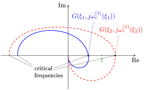
Figure 1: Illustration of Theorem 2 in the Nyquist plot. Full line: $G(\xi_{1},j\omega)$, dashed line: $G(\xi_{2},j\omega)$, both for $\omega\geq 0$. The theorem asserts existence of a Hopf bifurcation on any path between $\xi_{1}$ and $\xi_{2}$.

3.3 An algorithm for a numerical parameter search

In this section, we discuss an algorithm to search for parameter values that will lead to a change in stability properties of an equilibrium point. We assume that a starting parameter $p_{1}$ and a corresponding equilibrium $\bar{x}_{1}$ are known, which we combine in the pair $\xi_{1}=(\bar{x}_{1},p_{1})\in\mathcal{M}$. It is reasonable to assume that the pair $\xi_{1}$ is not critical, otherwise it is usually straightforward to find parameter values yielding equilibrium points with different stability properties. Moreover, the manifold $\mathcal{M}$ is assumed to be defined by a nonlinear equation of the form $\varphi(\xi)=0$. Often, one can directly use $\varphi=F$, but sometimes a modification is useful to exclude some solutions if the equation $F(x,p)=0$ is known to have multiple solutions. The aim of the algorithm is to find an equilibrium–parameter pair $\xi_{2}\in\mathcal{M}$ such that $\xi_{2}$ is not topologically equivalent to $\xi_{1}$. The main theoretical basis of the algorithm is the result of Theorem 2. Thus it is also possible to search specifically for either static or dynamic bifurcations on a path from $\xi_{1}$ to $\xi_{2}$ by choosing an appropriate critical frequency.

In order to put the problem in the framework developed in this paper, a loopbreaking for the system (1) has to be defined. Then, by looking at the resulting transfer function $G(\xi_{1},s)$, possible changes in stability properties can be determined. In particular one has to decide whether to search for a static or for a dynamic bifurcation. This leads to the choice of a critical frequency $\omega_{c}^{i}$ which is to be considered in the algorithm.

Denote the transfer function value for the critical frequency at a point $\xi$ as $\gamma(\xi)$. At the starting point $\xi_{1}$, this value can be computed as

$$\gamma(\xi_{1})=G(\xi_{1},j\omega_{c}^{i}(\xi_{1})).$$ (19)

Note that an analytical expression of the function $\gamma$ can be derived directly, maybe with the support of computer algebra for more complex systems. This derivation requires only basic algebraic manipulations, differentiation and matrix inversion, which can all be done symbolically for typical system classes. In particular, it is not required to have an analytical solution of the equation $F(x,p)=0$ to construct $\gamma$.

Now two cases have to be distinguished.

1. If $\gamma(\xi_{1})<1$, the algorithm searches a pair $\xi_{2}\in\mathcal{M}$ such that $\gamma(\xi_{2})>1$.

2. If $\gamma(\xi_{1})>1$, the algorithm searches $\xi_{2}\in\mathcal{M}$ such that $\gamma(\xi_{2})<1$.

The algorithm we are using is best described by the term gradient-directed continuation method. Continuation methods [Richter and DeCarlo, 1983] are popular in numerical bifurcation analysis, where they are used to trace the equilibrium curve in the combined state-parameter space. In our algorithm, continuation is used to stay on the manifold $\mathcal{M}$. However, a continuation method alone is not sufficient, as $\mathcal{M}$ is $m$-dimensional with typically $m>1$. Thus, the continuation is complemented with a gradient ascent or descent approach to achieve the desired value for $\gamma(\xi_{2})$.

Since the algorithm is based on Theorem 2, assumptions (A1) and (A2) need to be checked. Depending on the system under consideration, this may be a difficult problem globally over the equilibrium-parameter manifold $\mathcal{M}$. However, for the validity of the algorithm’s results it is sufficient that (A1) and (A2) are satisfied locally along the path used for the continuation. These checks can be directly included in the algorithm. If the assumptions are violated at one point, the algorithm issues a warning message. The results may still be valid, because (A1) and (A2) are only sufficient, but not necessary conditions for Theorem 2. However, the results need to be checked separately in this case.

In detail, the algorithm works as follows. We are discussing case 1 only, small extensions are required for dealing with both cases.

1. Initialisation. Set $\xi^{(0)}=\xi_{1}$. Choose numerical parameters: $\Delta\gamma$ for the minimal required change in $\gamma(\xi)$ per iteration, $\delta^{(0)}$ as the initial step size and $\delta_{min}$ ($\delta_{max}$) as minimal (maximal) step size.

2. Checking assumptions. (A1) is checked locally by computing the poles and zeros of $G(\xi^{(i)},s)$. (A2) is checked locally by computing the critical frequencies $\Omega_{c}(\xi^{(i)})$ and applying Proposition 4. If the assumptions are not satisfied, output a warning.

3. Prediction step. This step assures the desired increase in $\gamma(\xi)$.

   1. Compute the gradient $\nabla\gamma\left(\xi^{(i)}\right)$.

   2. Compute the subspace which is tangent to $\mathcal{M}$ in the point $\xi^{(i)}$:

      $$T_{\xi^{(i)}}\mathcal{M}=\operatorname{null}\frac{\partial\varphi}{\partial\xi}\left(\xi^{(i)}\right).$$ (20)

   3. Project $\nabla\gamma\left(\xi^{(i)}\right)$ on $T_{\xi^{(i)}}\mathcal{M}$:

      $$v^{(i)}=\operatorname{Proj}\left(\nabla\gamma\left(\xi^{(i)}\right),T_{\xi^{(i)}}\mathcal{M}\right).$$ (21)

   4. Set the predicted point

      $$\xi^{(i+1)}_{pre}=\xi^{(i)}+\delta^{(i)}v^{(i)}.$$ (22)

      Step size control is used in the sense that $\delta^{(i)}$ is varied to assure that the condition

      $$\gamma\left(\xi^{(i+1)}_{pre}\right)-\gamma\left(\xi^{(i)}\right)\geq\Delta\gamma$$ (23)

      is satisfied, while keeping $\delta_{min}\leq\delta^{(i)}\leq\delta_{max}$.

4. Correction step. Generally, $\xi^{(i+1)}_{pre}\notin\mathcal{M}$, so a correction step is required to achieve $\xi^{(i+1)}\in\mathcal{M}$. To this end, the Gauss-Newton method is used to solve the nonlinear equation

   $$\varphi(\xi^{(i+1)}) =0$$ (24)

   $$\gamma\left(\xi^{(i+1)}\right) =\gamma\left(\xi^{(i+1)}_{pre}\right)$$

   for $\xi^{(i+1)}$, where $\xi^{(i+1)}_{pre}$ is used as starting point for the Gauss-Newton algorithm. If the Gauss-Newton algorithm converges, the algorithm takes the solution as value for $\xi^{(i+1)}$ and proceeds to the next step. Otherwise, the algorithm reduces the step size $\delta^{(i)}$ and goes back to 2d).

5. Finishing criterion. Compute $\gamma\left(\xi^{(i+1)}\right)$. If $\gamma\left(\xi^{(i+1)}\right)>1$, finish successfully, otherwise iterate to step 2.

If the algorithm finishes successfully, it does so in a finite number of steps with a previously known upper bound due to step size control via inequality (23).

However, in the same way as classical continuation methods, the algorithm may fail if the Gauss-Newton algorithm in step 3 does not converge, and the step size $\delta^{(i)}$ may not be reduced further due to the constraint $\delta_{min}\leq\delta^{(i)}$ at the same time. This problem may appear if the system is numerically ill-conditioned, but can typically be avoided by choosing a smaller value for either $\Delta\gamma$ or for $\delta_{min}$, with the drawback of increased computational effort. Also, it can in general not be excluded that the function $\gamma(\xi)$ has local extrema, which may pose problems to the algorithm. Such problem may be detected numerically from the vector $v^{(i)}$ taking very small values. However, in several applications we have not encountered this problem so far.

The algorithm as described above does not consider constraints on the parameters $p$. Such constraints can be included by slight modifications in steps 2 and 3. If the border of the set $\mathcal{P}$ is approached during the iteration, the modified algorithm projects the gradient $\nabla\gamma\left(\xi^{(i)}\right)$ on the intersection of the tangent to $\mathcal{M}$ and the tangent to the border of $\mathcal{P}$. With additional step size control, a constraint violation is then avoided.

3.4 Discussion of the feedback loop approach

Two key steps in the approach we have taken are the transformation of the problem to the frequency domain and the consideration of the critical frequencies. These steps require an elaborate setup and therefore need to be well justified.

Approaching the given problem in the time domain would typically require to deal with the eigenvalues of the Jacobian $\frac{\partial F}{\partial x}$ on the considered manifold of equilibrium points. In particular, it would require to consider how the eigenvalues change if the parameters change. Going to the frequency domain will typically reduce the number of variables that are to be tracked with changes, because there are typically less critical frequencies than eigenvalues. For a minimum phase system, the number of critical frequencies is not more than the relative degree of the transfer function $G(\xi,s)$. Moreover, the position of eigenvalues has to be tracked in the two dimensions of the complex plane, whereas the transfer function values at critical frequencies are always real numbers. In particular, it would be difficult to estimate from the eigenvalues of the system for some starting parameters, which pair of eigenvalues should be pushed to the imaginary axis in order to obtain a Hopf bifurcation. Using the frequency domain approach, the critical frequency for which the transfer function value should be pushed towards 1 can typically be determined easily.

In classical bifurcation analysis, so called bifurcation test functions are used to check whether a bifurcation may occur when going from one parameter value to another one [Kuznetsov, 1995]. The test function $\Psi$ is defined such that $\Psi(\xi_{c})=0$ if the bifurcation that is tested for occurs at $\xi_{c}$. Bifurcations are detected by the test function $\Psi(\xi)$ changing sign when going from one point to the other, i.e. if $\Psi(\xi_{1})\Psi(\xi_{2})<0$, then a bifurcation occurs between $\xi_{1}$ and $\xi_{2}$. For bifurcations of codimension one, suitable test functions are known and are routinely used in numerical continuation algorithms. Note that in the frequency domain approach, the expression $G(\xi,j\omega_{c}(\xi))-1$ is a test function for a generic saddle-node bifurcation, if we consider $\omega_{c}=0$, and it is a test function for a generic Hopf bifurcation when considering $\omega_{c}\neq 0$. Computing classical test functions for a given point $\xi$ requires a similar or slightly less computational effort as computing the transfer function values at the critical frequency. So we need to justify why we do not use classical test functions for bifurcation search in a high-dimensional parameter space.

Because classical continuation methods cannot be used in a high-dimensional parameter space, one has to look for different approaches. A naive approach to find parameters for a bifurcation would be to solve directly the equations

$$\Psi(\xi) =0$$ (25)

$$F(\xi) =0.$$

However, in most cases this will be numerically infeasible with classical test functions, even if the combined parameter state space is of very low dimension. A more sophisticated approach could use basically the same algorithm that we have presented in Section 3.3, the gradient-directed continuation method, and just use the gradient of a classical bifurcation test function instead of the gradient of the transfer function $G(\xi,j\omega_{c}(\xi))$. We have also implemented this approach for several examples, but run into numerical problems for any system of medium complexity. In particular, the analysis presented in the next section did not work with a classical bifurcation test function for a Hopf bifurcation due to numerical problems. These problems seems to be related to our observation that the value of the classical bifurcation test function seems to be numerically much less well behaved with respect to parameter variations than the transfer function value at critical frequencies.

4 Application to a biological signalling system

In this section, we apply the theoretical results and the numerical algorithm described in the previous section to a system for biochemical signal transduction. A central element of the signal transduction in eukaryotic cells is the mitogen activated protein kinase (MAPK) cascade. It appears in several signalling pathways and is related to cell differentiation, proliferation, and response to external stress. Several ODE models for this system have been proposed during the last decade [Orton et al., 2005].

The MAPK cascade consists of three layers of kinase proteins, where each kinase activates the next layer, and the last layer corresponds to the output of the cascade. We consider the MAPK cascade as it appears in the EGF (epidermal growth factor) receptor pathway [Brightman and Fell, 2000]. There, the three kinases in the order how activation proceeds are Raf, MEK (MAPK/ERK kinase), and ERK (extracellular-signal-regulated kinase). Active ERK phosphorylates and inhibits SOS (son of sevenless homologue), which is required in the activation of Raf [Brightman and Fell, 2000]. This constitutes a negative feedback loop in the system. The model we use here is a slight simplification of a model suggested by Kholodenko [2000], and it is also a subsystem of the EGF pathway as modelled by Brightman and Fell [2000]. A cartoon of the biochemical reactions incorporated in the model is shown in Fig. 2.

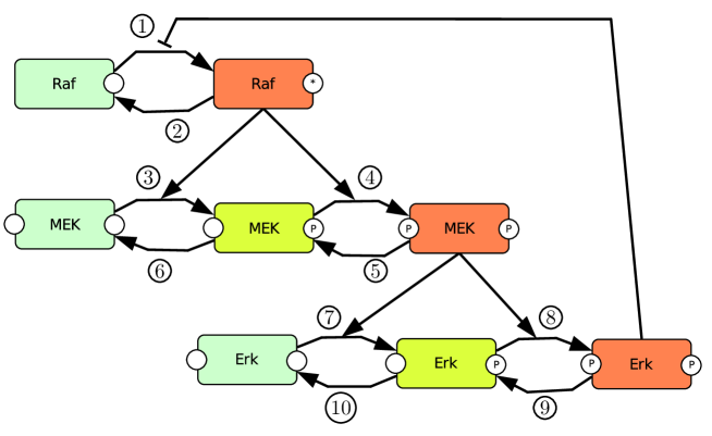
Figure 2: Illustration of the MAPK cascade model with reaction numbers.

In the equations, the concentrations of phosphorylated kinases are denoted as $x_{11}=$ [Raf*], $x_{21}=$ [MEK-P], $x_{22}=$ [MEK-PP], $x_{31}=$ [ERK-P] and $x_{32}=$ [ERK-PP]. The concentrations of unphosphorylated inactive kinases Raf, MEK and ERK need not be included as state variables, as they can be computed via the conservation laws

$$\textnormal{[Raf]}+x_{11} =x_{1t}$$

$$\textnormal{[MEK]}+x_{21}+x_{22} =x_{2t}$$

$$\textnormal{[ERK]}+x_{31}+x_{32} =x_{3t},$$

where $x_{1t}$, $x_{2t}$ and $x_{3t}$ are parameters for the total concentrations of kinases, which are constant. Table 1 shows the mathematical expressions for the reaction rates, with numbers corresponding to the labels in Fig. 2. Nominal parameter values for the simplified model have been adopted from [Kholodenko, 2000], and are shown in Table 2 as $p_{1}$.

Table 1: Reaction rates in the MAPK cascade model

Reaction	Rate
$v_{1}$	$V_{1}\frac{x_{1t}-x_{11}}{(1+x_{32}/K_{i})(K_{m1}+x_{1t}-x_{11})}$
$v_{2}$	$V_{2}\frac{x_{11}}{K_{m2}+x_{11}}$
$v_{3}$	$k_{3}x_{11}(x_{2t}-x_{21}-x_{22})$
$v_{4}$	$k_{4}x_{11}x_{21}$
$v_{5}$	$V_{5}\frac{x_{22}}{K_{m5}+x_{22}}$
$v_{6}$	$V_{6}\frac{x_{21}}{K_{m6}+x_{21}}$
$v_{7}$	$k_{7}x_{22}(x_{3t}-x_{31}-x_{32})$
$v_{8}$	$k_{8}x_{22}x_{31}$
$v_{9}$	$V_{9}\frac{x_{32}}{K_{m9}+x_{32}}$
$v_{10}$	$V_{10}\frac{x_{31}}{K_{m10}+x_{31}}$

Using the reaction rates from Table 1, the model can be written as a system of five ODEs with 20 parameters:

$$\dot{x}_{11} =v_{1}-v_{2}$$ (26)

$$\dot{x}_{21} =v_{3}+v_{5}-v_{4}-v_{6}$$

$$\dot{x}_{22} =v_{4}-v_{5}$$

$$\dot{x}_{31} =v_{7}+v_{9}-v_{8}-v_{10}$$

$$\dot{x}_{32} =v_{8}-v_{9}.$$

The only difference to Kholodenko’s model is in the phosphorylation reactions 3, 4, 7 and 8. The original model uses Michaelis-Menten kinetics for these reactions, whereas our simplified model uses mass action kinetics. It can be argued that with the concentrations of all kinases being on the same order of magnitude, the assumptions for using Michaelis-Menten kinetics in reactions 3, 4, 7 and 8 are not valid anyway, and one could aim to achieve a similar dynamical behaviour with the simpler model structure where mass action kinetics are used.

Kholodenko has shown in simulations that the system can show limit cycle oscillations for some parameter values. Due to the simplifications in four reaction rates, the model (26) does not oscillate for nominal parameter values $p_{1}$. Instead, the model has a stable equilibrium $\bar{x}_{1}$ for these parameter values. Solutions of the model converge to the steady state within $20$ seconds, as depicted in Fig. 3.

The question we deal with is whether parameters can be changed such that also the simplified model shows sustained oscillations. To answer this question, we apply the algorithm to search for critical parameter values which is described in the previous section.

The first step in our analysis is to choose a suitable loop breaking. For the given system, an intuitive approach is to break the loop at the feedback inhibition of reaction $v_{1}$ by ERK-PP. Thus we choose $h(x)=x_{32}$ and replace $x_{32}$ by the input $u$ in the reaction rate $v_{1}$, thus obtaining the dynamics of the open loop system $f(x,u,p)$.

A linearisation of the open loop system around the equilibrium point and a Laplace transformation give the transfer function $G(\xi,s)$, whose graph is shown in Fig. 4. The problem is now to find parameters $p_{2}$ with a corresponding unstable equilibrium point $\bar{x}_{2}$. This can be done using the numerical algorithm presented in Section 3.3.

The set of critical frequencies is minimal with $\alpha=3$, which can be seen from Fig. 4 by the observation that the graph of $G(\xi_{1},j\omega)$ encircles the origin monotonically and crosses the real axis three times. The origin of the complex plane is not counted as crossing, as we have $\omega=\pm\infty$ there. The only positive critical frequency is $\omega_{c}^{3}(\xi_{1})=0.017\,s^{-1}$, and we will consider only $\omega_{c}^{3}$ in the search for destabilising parameters, because our goal is to find a Hopf bifurcation. The corresponding transfer function value is $G(\xi_{1},j\omega_{c}^{3}(\xi_{1}))=\gamma(\xi_{1})=0.12$, corresponding to the equilibrium $\bar{x}_{1}$ being stable in the closed loop system.

The goal for the parameter search algorithm is to find parameters such that $\gamma(\xi_{2})>1$. Then the corresponding equilibrium point $\bar{x}_{2}$ will not be topologically equivalent to the nominal equilibrium $\bar{x}_{1}$ and we can expect a Hopf bifurcation when varying parameters from the nominal value $p_{1}$ to the new value $p_{2}$. To ensure that the algorithm does not stop at the bifurcation point, but continues to vary parameters until the oscillations have reached a considerable amplitude, we try to achieve $\gamma(\xi_{2})\geq 1.5$ in the implementation used here.

In the application of the algorithm to this problem, we set the minimal change in the transfer function value per iteration $\Delta\gamma=10^{-4}$ and the initial step size $\delta^{(0)}=10^{-4}$. The Gauss-Newton algorithm in the correction step was constrained to 20 iterations, but in the step size control the step size $\delta^{(i)}$ was already decreased if the Gauss-Newton algorithm required five or more iterations for convergence. With these settings the algorithm finishes successfully after 276 iterations, yielding the parameters $p_{2}$ and an equilibrium $\bar{x}_{2}$ with the transfer function value $G(\xi_{2},j\omega_{c}^{3}(\xi_{2}))=1.52$ and the critical frequency $\omega_{c}^{3}(\xi_{2})=0.0068\,s^{-1}$, where $\xi_{2}=(\bar{x}_{2},p_{2})$. The parameter values in $p_{2}$ are shown in Table 2. Note that although in principle all parameters could have been changed when going from $p_{1}$ to $p_{2}$, the algorithm varies only 9 out of the 20 parameters by an amount of more than 20 %. Since the algorithm uses the gradient of the transfer function value at the critical frequency, we can presume that the parameters that have been varied by a larger amount have higher influence on existence of oscillations than the other parameters.

Table 2: Reference parameters $p_{1}$ and parameters for instability $p_{2}$ in the MAPK cascade model.

Param.	$p_{1}$	$p_{2}$	Unit	rel. change
$V_{1}$	2.5	2.5	nM/s	$1.00$
$K_{i}$	9	18.9	nM	$2.09$
$K_{m1}$	10	8.1	nM	$1.23^{-1}$
$V_{2}$	0.25	0.17	nM/s	$1.43^{-1}$
$K_{m2}$	8	0.54	nM	$14.8^{-1}$
$k_{3}$	0.001	$4.3\cdot 10^{-4}$	1/(s nM)	$2.34^{-1}$
$k_{4}$	0.001	$5.7\cdot 10^{-4}$	1/(s nM)	$1.76^{-1}$
$V_{5}$	0.75	0.74	nM/s	$1.01^{-1}$
$K_{m5}$	15	7.6	nM	$1.98^{-1}$
$V_{6}$	0.75	0.77	nM/s	$1.02$
$K_{m6}$	15	13.9	nM	$1.08^{-1}$
$k_{7}$	0.001	$5.2\cdot 10^{-4}$	1/(s nM)	$1.93^{-1}$
$k_{8}$	0.001	$7.9\cdot 10^{-4}$	1/(s nM)	$1.27^{-1}$
$V_{9}$	0.5	0.49	nM/s	$1.02^{-1}$
$K_{m9}$	15	15.1	nM	$1.01$
$V_{10}$	0.5	0.51	nM/s	$1.01$
$K_{m10}$	15	15.4	nM	$1.03$
$x_{1t}$	100	100.2	nM	$1.00$
$x_{2t}$	300	300.2	nM	$1.00$
$x_{3t}$	300	304.4	nM	$1.01$

The graph of $G(\xi_{2},j\omega)$ is shown in Figure 4. For the new parameters $p_{2}$, the graph now encircles the point 1. By Theorem 1, we see that the equilibria $\bar{x}_{1}$ and $\bar{x}_{2}$ are not topologically equivalent. Indeed, $\bar{x}_{2}$ is unstable and the system converges to a limit cycle for parameters $p_{2}$. The time course of these oscillations is plotted in Figure 3.

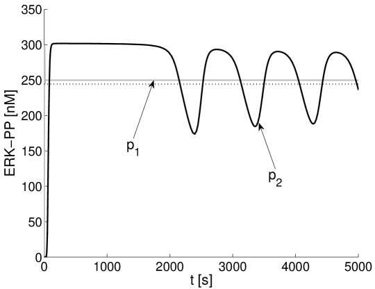
Figure 3: Convergence to steady state for parameters $p_{1}$ (grey line) and sustained oscillations for parameters $p_{2}$ (black line). The oscillations coexist with the unstable equilibrium $\bar{x}_{2}$ (dotted line).

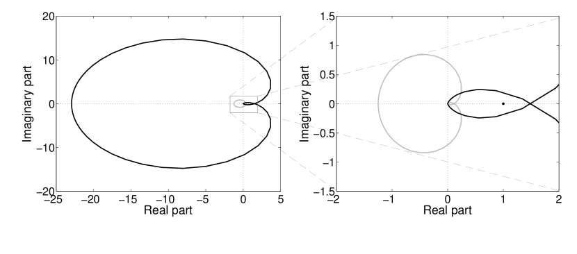
Figure 4: Nyquist plots of open–loop MAPK model for parameters $p_{1}$ (grey line) and $p_{2}$ (black line).

In conclusion, our method is able to compute parameters which render the corresponding equilibrium unstable and thus lead to the emergence of sustained oscillations in the treated example. About half of the parameters are varied by a non–negligible amount, but all variations are within the physiological range, the highest variation being a factor of about $15$ in the $K_{m}$-value of one reaction. It is also worth mentioning that the concentration values in the equilibrium did not change significantly, although this should not be of physiological relevance for the unstable equilibrium.

5 Conclusions

The loop breaking concept is introduced as a theoretical tool to analyse complex behaviour in ODE systems as frequently encountered in mathematical biology. Based on this tool, we present results on topological equivalence of equilibria in systems with high-dimensional parameter spaces and on the existence of critical parameters, for which stability properties of equilibria may change. In addition, an algorithm is given to systematically search for critical parameters. Using an ODE model for a MAPK cascade, we show that the algorithm can be used to efficiently search for parameter values leading to limit cycle oscillations in the system.

Non-uniqueness of critical parameter values is a problem that is inherent to this kind of analysis. If the dimension of the parameter space is higher than the codimension of the bifurcation, then there will be a submanifold of bifurcation points in the parameter space. Our algorithm computes one of these points. Starting from a critical point thus found, one can then use continuation methods to further explore the structure of the set of critical points.

Another possibility for further studies would be to search for a bifurcation which is locally closest to some reference parameter values. A method for this has been presented by Dobson [2003]. The method requires a bifurcation point where the search is started, and we expect our algorithm to give a starting point which is better suited for the method discussed in [Dobson, 2003] than a bifurcation search along a random line in parameter space.

The biological example we study in Section 4 is simple in that it contains only one feedback loop. For systems with a single feedback loop, the results of the proposed analysis method are independent of how the loop breaking point is chosen. Of course many biological systems contain several intertwined feedback loops. Then, the choice of the loop breaking point needs more attention, because the results in general depend on this choice. In our experience, it is often beneficial to try to break several feedback loops at once. Also a comparison of different loop breaking points is usually helpful and could give hints to the role played by individual loops in the dynamical behaviour of the system.

Appendix

Proof of Lemma 1

For simplicity of notation, we drop the dependence on $\xi$ of matrices $A$, $B$ and $C$. By Schur’s lemma, we have

$$\operatorname{det}(sI-A_{cl})=\operatorname{det}(sI-A-BC)=\operatorname{det}\begin{pmatrix}sI-A&-B\\ -C&1\end{pmatrix}.$$

Let $(sI-A)_{-i}\in\mathbb{R}^{(n-1)\times n}$ denote the matrix $(sI-A)$ with the $i$-th row deleted. Then, by cofactor expansion,

$$\operatorname{det}\begin{pmatrix}sI-A&-B\\ -C&1\end{pmatrix}=1\cdot\operatorname{det}(sI-A)-\sum_{i=1}^{n}(-1)^{n+1+i}b_{i}\operatorname{det}\begin{pmatrix}(sI-A)_{-i}\\ -C\end{pmatrix}.$$

In the same way,

$$\operatorname{det}\begin{pmatrix}sI-A&-B\\ -C&0\end{pmatrix}=-\sum_{i=1}^{n}(-1)^{n+1+i}b_{i}\operatorname{det}\begin{pmatrix}(sI-A)_{-i}\\ -C\end{pmatrix}$$

and with Prop. 1 it follows that

$$\operatorname{det}(sI-A_{cl})=\operatorname{det}(sI-A)-\operatorname{det}\begin{pmatrix}sI-A&-B\\ C&0\end{pmatrix}.$$ (27)

$s_{0}$ is an eigenvalue of $A_{cl}$ if and only if $\operatorname{det}(s_{0}I-A_{cl})=0$. For condition (i), we have $\operatorname{det}(s_{0}I-A)\neq 0$, and thus the equation

$$\frac{\operatorname{det}\begin{pmatrix}s_{0}I-A&-B\\ C&0\end{pmatrix}}{\operatorname{det}(s_{0}I-A)}=1$$

is equivalent to $s_{0}$ being an eigenvalue of $A_{cl}$. The claim then follows from (8).

The other case where $\operatorname{det}(s_{0}I-A)=0$ is considered in condition (ii), and (27) can be used directly to prove the claim.

Proof of Proposition 4

Note that $\alpha$ is constant over $\mathcal{M}$ due to assumption (A1). Consider the transfer function $G(\xi,s)$ for a constant $\xi\in\mathcal{M}$. For ease of notation, we drop $\xi$ in the transfer function in the following.

It is well known from linear control theory that the argument of $G(j\omega)$ changes by $\alpha\pi$ when varying $\omega$ from $-\infty$ to $\infty$ D’Azzo and Houpis [1975]:

$$|\arg G(j\infty)-\arg G(-j\infty)|=\alpha\pi.$$

The symmetry $G(j\omega)=\overline{G(-j\omega)}$ implies that $\arg G(j\infty)=-\arg G(-j\infty)$. From these two facts, it follows that the argument of $G(j\omega)$ spans the open interval $I_{\alpha}=(-\frac{\alpha\pi}{2},\frac{\alpha\pi}{2})$ for $\omega\in(-\infty,\infty)$.

Moreover, by Definition 2 the condition $\omega_{c}\in\Omega_{c}(\xi)$ is equivalent to

$$\arg G(j\omega_{c})=k\pi,\qquad k\in\mathbb{Z}.$$

If $\alpha$ is even, the claim follows directly, since there are $\alpha-1$ different integer values for $k$ such that $k\pi$ is inside the interval $I_{\alpha}$. This corresponds directly to having $\alpha-1$ or more critical frequencies.

In the other case, if $\alpha$ is odd, some additional reasoning is needed to prove the proposition. In this case one has

$$I_{\alpha}=\left(-\frac{2m+1}{2}\pi,\frac{2m+1}{2}\pi\right),\qquad m\in\mathbb{Z}.$$

Thus the borders of the interval $I_{\alpha}$ are not at integer multiples of $\pi$, which implies that in this case there are $\alpha$ different integer values for $k$ such that $k\pi$ is in $I_{\alpha}$, corresponding to at least $\alpha$ critical frequencies.

Proof of Theorem 1

The proof for Theorem 1 uses the argument principle from complex analysis, which is repeated here for completeness [Whittaker and Watson, 1965].

Theorem (The argument principle):

Let $f$ be a meromorphic function on the domain $D\subset\mathbb{C}$ and $\Gamma$ a simply closed curve in $D$ such that $f$ does not have a zero or pole on $\Gamma$. The winding number $wn(f(\Gamma),0)$ of the image of $\Gamma$ under $f$ around the origin is given by

$$wn(f(\Gamma),0)=z_{f}-p_{f},$$

where $z_{f}$ ($p_{f}$) is the number of zeros (poles) of $f$ in the interior of the curve $\Gamma$, counted according to their algebraic multiplicities.

Note that the winding number is counted in the counter-clockwise direction.

As typically done in linear control theory, we will generally use the imaginary axis for $\Gamma$, also called the Nyquist curve. This can be seen as a closed curve by first taking only the interval $[-jR,jR]$ and the half circle with radius $R$ in the right half plane, and second letting $R\rightarrow\infty$. Thus the interior of $\Gamma$ is the right half plane.

We will first proof the intermediate results given in Lemmas 2–4, before proving Theorem 1.

Proof.

(Lemma 2) If $\Omega_{c}(\xi)$ is minimal, then there is exactly one $\omega_{c}\in\Omega_{c}(\xi)$ such that $\arg G(\xi,j\omega_{c})=k\pi$ for each $k\in\mathbb{Z}$ with $k\pi\in I_{\alpha}$ (where $I_{\alpha}$ is the interval defined in the proof of Proposition 4). This implies that

$$\left|\arg G(\xi,j\omega_{c}^{i}(\xi))-\arg G(\xi,j\omega_{c}^{i-1}(\xi))\right|=\pi$$

and thus $G(\xi,j\omega_{c}^{i}(\xi))G(\xi,j\omega_{c}^{i-1}(\xi))<0$. ∎

Proof.

(Lemma 3) Note that the loop breaking (4) assures that $G(\xi,j\infty)=G(\xi,-j\infty)=0$. Considering also Lemma 2, it follows that every cut of $G(\xi_{i},\Gamma)$ to the right of the point $1$ is preceded and followed by a cut of $G(\xi_{i},\Gamma)$ with the negative real axis. Thus each cut to the right of the point $1$ corresponds to one winding of $G(\xi_{1},\Gamma)$ around the point $1$. Moreover, Lemma 2 assures that these windings all have the same direction and thus several windings cannot cancel in the total winding number. ∎

Proof.

(Lemma 4) From assumption (A1), the transfer functions $G(\xi_{1},\cdot)$ and $G(\xi_{2},\cdot)$ have the same number of zeros and poles in the left and right half plane. Thus for the phase differences we have

$$\arg G(\xi_{1},j\infty)-\arg G(\xi_{1},-j\infty)=\arg G(\xi_{2},j\infty)-\arg G(\xi_{2},-j\infty).$$

This implies that the winding numbers $wn(G(\xi_{1},\Gamma),1)$ and $wn(G(\xi_{2},\Gamma),1)$ have the same sign and with Lemma 3 we conclude

$$\big{|}wn(G(\xi_{1},\Gamma),1)-wn(G(\xi_{2},\Gamma),1)\big{|} =\big{|}|wn(G(\xi_{1},\Gamma),1)|-|wn(G(\xi_{2},\Gamma),1)|\big{|}$$

$$=\big{|}\beta(\xi_{1})-\beta(\xi_{2})\big{|}.$$

∎

We are now ready to give the proof of Theorem 1.

Proof.

(Theorem 1) By Definition 4, topological equivalence of $\xi_{1}$ and $\xi_{2}$ is equivalent to the condition that the matrices $A_{cl}(\xi_{1})$ and $A_{cl}(\xi_{2})$ have the same number of eigenvalues with positive real part.

From the proof of Lemma 1, we know that

$$G(\xi,s)-1=\frac{\operatorname{det}(sI-A_{cl}(\xi))}{\operatorname{det}(sI-A(\xi))}.$$

Using the argument principle, it follows that

$$wn(G(\xi,\Gamma),1)=n_{cl}(\xi)-n_{ol}(\xi),$$

where $n_{cl}(\xi)$ ($n_{ol}(\xi)$) is the number of eigenvalues of $A_{cl}(\xi)$ ($A(\xi)$) with positive real part. By assumption, $n_{ol}(\xi_{1})=n_{ol}(\xi_{2})$ and thus $\xi_{1}$ and $\xi_{2}$ are topologically equivalent if and only if

$$wn(G(\xi_{1},\Gamma),1)=wn(G(\xi_{2},\Gamma),1).$$

The claim of the theorem then follows from Lemma 4. ∎

Biographical information

Steffen Waldherr is research assistant at the Institute for Systems Theory and Automatic Control at the University of Stuttgart, Germany. His main research interests are uncertainty analysis of biochemical reaction networks, non-linear dynamics, and modelling of biochemical signal transduction pathways.

Frank Allgöwer is director of the Institute for Systems Theory and Automatic Control at the University of Stuttgart, Germany. His main research interests are nonlinear, robust, and predictive control, identification, and applications in process engineering, systems biology, mechatronics, and nanotechnology.

References

- Allwright [1977] D. J. Allwright. Harmonic balance and the Hopf bifurcation theorem. Math. Proc. Cambridge Philos. Soc., 82:81–127, 1977.
- Brightman and Fell [2000] F. A. Brightman and D. A. Fell. Differential feedback regulation of the MAPK cascade underlies the quantitative differences in EGF and NGF signalling in PC12 cells. FEBS Lett., 482:169–174, 2000.
- Cinquin and Demongeot [2002] O. Cinquin and J. Demongeot. Positive and negative feedback: striking a balance between necessary antagonists. J. Theor. Biol., 216(2):229–241, May 2002. 10.1006/jtbi.2002.2544. URL http://dx.doi.org/10.1006/jtbi.2002.2544.
- D’Azzo and Houpis [1975] J. J. D’Azzo and C. H. Houpis. Linear Control Sytem Analysis and Design: Conventional and Modern. McGraw-Hill, New York, 1975.
- Dobson [2003] I. Dobson. Distance to bifurcation in multidimensional parameter space: Margin sensitivity and closest bifurcations. In G. Chen, D. J. Hill, and X. Yu, editors, Bifurcation Control, Theory and Applications, volume 293 of LNCIS, pages 49–66. Springer-Verlag, Berlin, 2003.
- Eissing et al. [2004] T. Eissing, H. Conzelmann, E. D. Gilles, F. Allgöwer, E. Bullinger, and P. Scheurich. Bistability analyses of a caspase activation model for receptor-induced apoptosis. J. Biol. Chem., 279(35):36892–97, August 2004.
- Ferrell and Xiong [2001] J. E. Ferrell and W. Xiong. Bistability in cell signaling: How to make continuous processes discontinuous, and reversible processes irreversible. Chaos, 11(1):227–236, Mar 2001. 10.1063/1.1349894. URL http://dx.doi.org/10.1063/1.1349894.
- Henderson [2007] M. E. Henderson. Higher-dimensional continuation. In B. Krauskopf, editor, Numerical continuation methods for dynamical systems, pages 77–115. Springer, Dordrecht, 2007.
- Kaufman et al. [2007] M. Kaufman, C. Soule, and R. Thomas. A new necessary condition on interaction graphs for multistationarity. J. Theor. Biol., 248(4):675–685, Oct 2007. URL http://www.sciencedirect.com/science/article/B6WMD-4P29KKM-1/2/a2ed23af%e670339baa01d371ef7daf4e.
- Kholodenko [2000] B. N. Kholodenko. Negative feedback and ultrasensitivity can bring about oscillations in the mitogen-activated protein kinase cascades. Eur. J. Biochem., 267(6):1583–88, Mar 2000.
- Kim et al. [2006] J. Kim, D. G. Bates, I. Postlethwaite, L. Ma, and P. A. Iglesias. Robustness analysis of biochemical network models. IEE Proc. Syst. Biol., 153(3):96–104, May 2006.
- Kuznetsov [1995] Y. A. Kuznetsov. Elements of Applied Bifurcation Theory. Springer-Verlag, New York, 1995.
- Leloup and Goldbeter [2003] J.-C. Leloup and A. Goldbeter. Toward a detailed computational model for the mammalian circadian clock. Proc. Natl. Acad. Sci., 100(12):7051–56, Jun 2003. 10.1073/pnas.1132112100. URL http://dx.doi.org/10.1073/pnas.1132112100.
- Lu et al. [2006] J. Lu, H. Engl, and P. Schuster. Inverse bifurcation analysis: Application to simple gene systems. Algorithms Mol. Biol., 1(1):11, Jul 2006. 10.1186/1748-7188-1-11. URL http://dx.doi.org/10.1186/1748-7188-1-11.
- Mees and Chua [1979] A. I. Mees and L. O. Chua. The Hopf bifurcation theorem and its applications to non-linear oscillations in circuits and systems. IEEE Trans. Circ. Syst., 26(4):235–254, 1979.
- Moiola et al. [1991] J. Moiola, A. Desages, and J. Romagnoli. Computing bifurcation points via characteristic gain loci. IEEE Trans. Autom. Control, 36(3):358–362, 1991. ISSN 0018-9286.
- Moiola et al. [1997] J. L. Moiola, M. C. Colantonio, and P. D. Donate. Analysis of static and dynamic bifurcations from a feedback systems perspective. Dyn. Stab. Syst., 12(4):293–317, December 1997.
- Mönnigmann and Marquardt [2002] M. Mönnigmann and W. Marquardt. Normal vectors on manifolds of critical points for parametric robustness of equilibrium solutions of ODE systems. J. of Nonlin. Sci., 12(2):85–112, 2002.
- Orton et al. [2005] R. J. Orton, O. E. Sturm, V. Vyshemirsky, M. Calder, D. R. Gilbert, and W. Kolch. Computational modelling of the receptor-tyrosine-kinase-activated MAPK pathway. Biochem. J., 392(Pt 2):249–261, Dec 2005. 10.1042/BJ20050908. URL http://dx.doi.org/10.1042/BJ20050908.
- Richter and DeCarlo [1983] S. L. Richter and R. A. DeCarlo. Continuation methods: theory and applications. IEEE Trans. Circ. Syst., 30(6):347–352, 1983.
- Skogestad and Postlethwaite [1996] S. Skogestad and I. Postlethwaite. Multivariable Feedback Control. Analysis and Design. John Wiley & Sons, Chichester, 1996.
- Snoussi [1998] E. H. Snoussi. Necessary conditions for multistationarity and stable periodicity. J. Biol. Syst., 6:3–9, 1998.
- Stelling et al. [2004] J. Stelling, U. Sauer, Z. Szallasi, F. J. Doyle, and J. Doyle. Robustness of cellular functions. Cell, 118(6):675–685, Sep 2004. 10.1016/j.cell.2004.09.008. URL http://dx.doi.org/10.1016/j.cell.2004.09.008.
- Stiefs et al. [2008] Dirk Stiefs, Thilo Gross, Ralf Steuer, and Ulrike Feudel. Computation and visualization of bifurcation surfaces. Int. J. Bif. Chaos, 18(8):2191–2206, Aug 2008.
- Whittaker and Watson [1965] E. T. Whittaker and G. N. Watson. A Course of Modern Analysis. Cambridge University Press, Cambridge, UK, 1965. Reprint of the 4th edition.