Universal Correlations and Dynamic Disorder in a Nonlinear Periodic 1D System

Abstract

When a periodic 1D system described by a tight-binding model is uniformly initialized with equal amplitudes at all sites, yet with completely random phases, it evolves into a thermal distribution with no spatial correlations. However, when the system is nonlinear, correlations are spontaneously formed. We find that for strong nonlinearities, the intensity histograms approach a narrow Gaussian distributed around their mean and phase correlations are formed between neighboring sites. Sites tend to be out-of-phase for a positive nonlinearity and in-phase for a negative one. The field correlations take a universal shape independent of parameters. This nonlinear evolution produces an effectively dynamically disordered potential which exhibits interesting diffusive behavior.

The tight binding approximation is one of the simplest models that predict band structure and ballistic motion in periodic systems bloch . Using a tight-binding model with disorder, P.W. Anderson was able to predict and study the effect of localization in disordered lattices anderson . A nonlinear version of the tight-binding model, better known as the Discrete Nonlinear Schrödinger Equation (DNLSE) has been used to study nonlinear evolution in periodic systems, initially in the context of periodic molecular and mechanical systems scott , and extensively in recent years to describe nonlinear propagation in optical waveguide lattices christodoulides ; lederer , as well as matter-waves in light-induced latticesBEC . In particular, the DNLSE explains the formation of nonlinear intrinsic localized modes, also known as discrete solitons chandjoseph or discrete breathers flach . Disorder and localization have been studied experimentally recently both in matter-waves aspect ingucio and in photonic lattices segev ; lahini . An issue of particular interest and some debate is the interplay between localization and nonlinearity shepelyansky ; flach1 .

Here we report on a new phenomenon that results from the interplay of nonlinearity and disorder. This effect occurs in periodic systems, where nonlinearity induces disorder in an otherwise perfectly ordered lattice. What we find is that when the system is initialized with random-phase fields, it evolves into particular distributions with well defined stationary statistical properties. Most interestingly, the field correlation function and the distribution of phases assume universal forms independent of the exact value of the nonlinear parameter. The resulting distribution induces a dynamic structure with several intriguing properties.

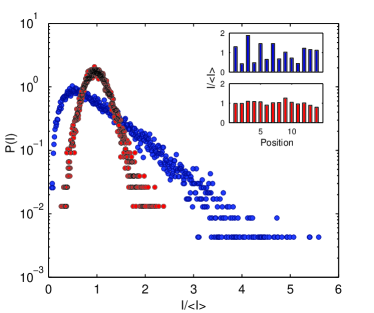
Figure 1: Experimental measurement of output light intensities from a waveguide array, when input fields with equal amplitudes, yet random phases, are coupled to several adjacent waveguides. Measured values of many random-phase realizations are shown as histograms for linear propagation (blue circles) and high-intensity, nonlinear propagation (red circles). The inset shows two sets of measurements for an input with the same phase realization after linear (blue) and nonlinear (red) propagation. The output intensity distribution is exponential-like in linear propagation, and becomes narrow, Gaussian-like in the nonlinear case.

In Fig. 1 we show the results of an optical experiment in a waveguide array that motivated this study. Light with uniform intensity yet random phases was injected into a large number of waveguides in a periodic waveguide lattice. The intensity at the output end was measured, and the histograms of intensity values obtained from many repeats of the experiment with different random phase realizations are shown for both low intensity and high intensity light. For experimental details, see Methods below. While linear propagation produced exponential-like distribution of intensities, as expected for summing of many random-phase inputs, the nonlinear propagation yielded a much narrower distribution around the average intensity. Increasing the optical power led to the narrowing of the output distribution. Note that for both measurements, the counts at low intensity values are underestimated because of scattered light and instrumentation noise. To investigate this behavior we have modeled the problem using the DNLSE. While we use here the notations of optics, our results will hold in general for all other systems described by the DNLSE. The evolution of light in a periodic array of weakly coupled waveguides is described by:

$$i\frac{da_{n}}{dz}=C(a_{n-1}+a_{n+1})+\gamma|a_{n}|^{2}a_{n},$$ (1)

where $a_{n}$ is the amplitude of the mode in the $n^{th}$ waveguide, C is the coupling coefficient to the nearest neighbors and $\gamma$ is the nonlinear coefficient, positive (negative) for focusing (defocusing) nonlinearity. We shall consider the situation where light is injected into the array with uniform amplitudes $|a_{n}|=a_{0}$, yet with completely uncorrelated, random phases. It is convenient to use the normalized equation,

$$i\frac{du_{n}}{d\zeta}=(u_{n-1}+u_{n+1})+\Gamma|u_{n}|^{2}u_{n},$$ (2)

where $\zeta=zC$, $u_{n}=a_{n}/a_{0}$ and $\Gamma=\gamma{a_{0}}^{2}/C$. With this normalization, the input intensities are all uniform with $I_{n}(0)=u_{n}{u_{n}}^{*}=1$.

Consider first the linear problem, i.e. $\Gamma=0$. As might be expected, after a certain distance, mixing of the different input fields leads to an output pattern with fluctuating intensities. Fig. 2(a)-(c) shows results of numerical simulations of Eq. (2) for various properties of the fields after propagating a distance of $\zeta=10$ in an array with $N=256$ waveguides. Periodic boundary conditions are used to avoid edge effects. The results shown are averaged over 500 realizations with different random initial fields. Fig. 2(a) shows the intensity histogram; it follows an exponential law, $P(I)=\exp(-I)$, as expected for random fields. Fig. 1(b) shows the field correlations $C_{k}=\sum(u_{n}u_{n+k}^{*}+u_{n}^{*}u_{n+k})/2N$ demonstrating, as could be expected, that the fields at different sites do not correlate. Finally, Fig 1(c) shows the histogram of phase differences between neighbors, $\theta_{n}=\phi_{n}-\phi_{n+1}$, with $\phi_{n}=\arg u_{n}$ the phase of the field $u_{n}$. These phases are uniformly distributed.

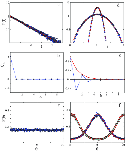
Figure 2: Simulation results of the DNLSE with uniform intensities and random phases. (a) Intensity histogram, (b) field correlation and (c) phase-difference histogram for a linear system ($\Gamma=0$), exhibiting exponential intensity distribution and uncorrelated fields and phases. (d) Intensity histograms for $\Gamma=\pm 20$ (blue circles) and $\Gamma=\pm 200$ (red circles). The distributions are narrower at higher nonlinearities, yet independent of the sign of $\Gamma$. (e) The universal field correlation function is identical for both nonlinear values, but depends on their sign: blue for positive (focusing, $\Gamma>0$), red for negative nonlinearities. (f) Phase difference histograms also approach a universal distribution, concentrating around $\pi$ for positive nonlinearity and 0 for the negative case. The theoretical lines in (d)-(f) are predictions of Eqs. (7) and (8).

We now repeat the simulations with nonlinearity, and we will be interested mostly in the limit of strong nonlinearity; results for $\Gamma=\pm 20$ and for $\Gamma=\pm 200$ are given in Figs. 2(d)-(f). Two changes from the linear case are obvious. First, the intensity histograms, shown in Fig. 2(d), now converge around the average intensity value of 1, with a width that shrinks with the nonlinear parameter. The distribution seems to fit well a gaussian distribution with $P(I)=\exp[-(I-1)^{2}/2\sigma^{2}]$, and it is independent of the sign of the nonlinearity.

The second major effect of the nonlinearity is the induced spatial field correlations. Most interestingly, the correlation function (Fig. 2(e)) takes a shape that is independent of the nonlinearity value, and is sensitive only to its sign. It is described well by exponential decays, $C_{k}=(-1)^{k}\exp(-\alpha k)$ for positive (focusing) nonlinearity and $C_{k}=\exp(-\alpha k)$ for the negative case. Note that the correlation is only visible in the fields - the intensities remain uncorrelated; Intensity correlations show a diminished peak at k=0 and a uniform background. These field patterns are consistent with the known properties of modulation instability in such systems: Staggered (unstaggered) fields are stable in positive (negative) nonlinearity arrays modulation .

Since the intensities become more uniform at high nonlinearities, the field correlation functions are dictated by the variations of phases between neighboring sites. In Fig. 1(f) we show the histograms of these phase differences for positive and negative nonlinearities. While in the former neighboring waveguides are most likely to be out of phase, as the distribution peaks at $\pi$, in the latter two neighboring waveguides tend to be in-phase. This distribution of phases also attains a constant profile at high nonlinearity values.

The field correlation and the intensity distribution are closely related. This can be deduced from the conserved quantities, the Hamiltonian

$$H=\frac{1}{2}\Gamma\sum I_{n}^{2}+\sum(u_{n}u_{n+1}^{*}+u_{n}^{*}u_{n+1}),$$ (3)

and the total photon number,

$$A=\sum I_{n}.$$ (4)

From these it is easy to show that

$$\frac{\Gamma}{4}\sigma^{2}(\zeta)+C_{1}(\zeta)=H_{0}$$ (5)

is also constant. Here $\sigma=(\Sigma I_{n}^{2}/N-1)^{1/2}$ is the standard deviation of the intensities. Since our initial condition are of uniform intensities, $\sigma^{2}(0)=0$, and random phases, $C_{1}(0)\approx 0$, then $H_{0}=0$, hence

$$\frac{\Gamma}{4}\sigma^{2}(\zeta)=-C_{1}(\zeta).$$ (6)

Equation (6) predicts that the signs of $C_{1}$ and $\Gamma$ are different, as indeed is observed in Fig 2. For weak nonlinearity ($\Gamma\ll 1$), when the distribution deviate only slightly from exponential, a small correlation is formed with $C_{1}=-\Gamma/4$. However, as the nonlinearity increases, Eq. (6) predicts that the intensity distribution has to narrow down, since necessarily $|C_{1}|<1$.

To relate the phase and intensity fluctuations, we have to study the statistical properties of the DNLSE. Such investigations were carried out by Rasmussen et al rasmussen , and extended later by Rumpf rumpf . They were mostly interested in the conditions for the generation of localized structures. With our initial conditions, it can be shown that localized structures are not formed, but we can use the same formalism to derive the probability distributions for phase and intensities.

In essence, the state of maximal entropy $S[p(I_{1},...I_{N},\theta_{1},...\theta_{N})]=-\int p\ln p\prod dI_{i}d\theta_{i}$ can be derived by the variational problem $\delta(S-\alpha A-\eta H-\lambda\int p)=0$, where $\alpha,\eta$ and $\lambda$ are the appropriate Lagrange multipliers rumpf . The problem is greatly simplified by the approximation $\Sigma(u_{n}u_{n+1}^{*}+c.c.)\approx 2\sum\cos(\theta_{n})$, which is consistent with the observation that the intensities are uncorrelated and at high nonlinearities they are close to their average value of 1. With this approximation, the intensities and phases are separable, and their distributions are derived to be:

$$p_{I}(I) = \lambda_{1}\exp[-\frac{\eta\Gamma}{2}(I-1)^{2}]$$ (7)

$$p_{\theta}(\theta) = \lambda_{2}\exp[-2\eta\cos(\theta)]$$ (8)

with $\lambda_{1},\lambda_{2}$ appropriate normalization constants and $\eta\approx\pm 0.533$ is the solution of $4\eta\int\cos(\theta)p_{\theta}(\theta)d\theta+1=0$, where the sign is selected to match the sign of $\Gamma$. The phase distribution is then maximized at $\theta=\pi$ ($\theta=0$) for positive (negative) $\Gamma,$ respectively. Note that these universal phase distribution functions, which are shown as lines in Fig 2(f), are independent of the value of the nonlinearity. They lead to the universal correlation function that decays with $C_{k}/C_{k+1}=-4\eta$ as shown in Fig 2(e).

Finally, we would like to discuss the potential (or index) pattern which is induced by the fluctuating fields through the nonlinear effect. The fields induce an effective dynamic disorder into the lattice; While we have shown above that the variations in intensities tend to diminish at high nonlinearities [$\sigma=(\eta\Gamma)^{-1/2}$], the variations in induced nonlinear potential, i.e. $\Gamma\sigma$ actually increase. The array becomes effectively more disordered: A stationary structure with this level of disorder would have been characterized by a localization length that is narrower than the lattice spacing. However, this increase in disorder is also accompanied by faster dynamics: The induced pattern changes faster at higher nonlinearities. The nonlinear potential map $\Gamma I_{n}(\zeta)$ is shown in Fig. 3, together with the intensity correlation maps $Y(k,\delta\zeta)=\Sigma_{n}\int d\zeta I_{n}(\zeta)I_{n-k}(\zeta-\delta\zeta)$. Note that while at a given $\zeta$ the intensities at adjacent waveguide do not correlate, $Y(k,0)=\delta_{k,0}$, they are correlated at other values of $\zeta$. It is this dynamic potential structure that determines the field correlations and other peculiarities of this system.

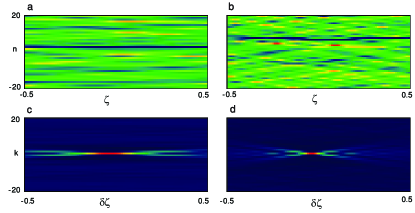
Figure 3: Maps of nonlinear potential induced by the fluctuating fields for (a) $\Gamma=20$ and (b) $\Gamma=200$ and the corresponding correlation maps $Y(k,\delta\zeta)$ (c,d). The maps show a section of 40 waveguides (vertically) and a propagation of $\zeta=1$. Note the faster dynamics for the higher nonlinearity, evident also in the correlation map. For easy viewing, the potentials are normalized to their peaks, although the values in (b) are about 3 times higher than in (a)

One way to characterize this structure is to investigate the transport properties of a a secondary probe beam that propagates in the nonlinearly induced disordered potential. We have simulated the propagation of such a weak probe field in an array with 1024 sites. The probe is launched into a single central site at $\zeta=0$, and its width is monitored along propagation. Fig. 4(a) shows this width, averaged over several realizations, as a function of $\zeta^{1/2}$, for two values of nonlinearity, $\Gamma=20$ and $\Gamma=200$, and Fig 4(b) shows the probe intensity distribution at $\zeta=2000$. It seems that the broadening is governed mostly by diffusive dynamics, that is, a gaussian-like distribution that broadens diffusively as $\zeta^{1/2}$. Indeed, dynamic disorder that is spatially uncorrelated is known to lead to diffusive broadening dynamic1 ; dynamic2 . What we find interesting is that at higher nonlinearities the diffusion coefficient is actually larger, in spite of the stronger disorder. This is most likely the result of the faster dynamics, but it could be that the nontrivial correlation maps also plays a role. These points are currently under investigation.

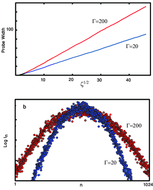
Figure 4: The diffusion of a weak probe in the nonlinear potential induced by the fluctuating fields with $\Gamma=20$ and $\Gamma=200$. (a) the averaged probe width as a function of $\zeta^{1/2}$. (b) The averaged probe profile at $\zeta=2000$

.

In conclusion, we have shown that when systems described by the DNLSE are initialized with equal amplitudes yet random phases, universal field and phase correlation are formed in the high nonlinearity limit. In contrast with the thermal distribution of intensities obtained in linear propagation, the intensity variations are diminished, and universal phase correlations are formed. The underlying potential field leading to this behavior is of a dynamic disordered system, which is characterized by diffusive propagation.

Methods: The periodic waveguide lattices were prepared on an AlGaAs substrate using e-beam lithography, followed by reactive ion etching. The width of each of the waveguides as well as their spacing were 4 microns. The tunneling parameter between sites C was measured to be $280m^{-1}$. The light source was a pulsed optical parametric amplifier, producing 1.2 ps pulses at a wavelength of 1530nm with a 1 KHz repetition rate. The spatial phase of the laser light beam was randomized using a computer-controlled spatial light modulator. The beam was shaped using a cylindrical optics and then injected into the input facet of the array, covering  15 lattice sites. The light intensity profile was measured at the output facet of the 8mm long sample using an infrared camera and the intensity statistics was calculated by collecting many such images with random phase realizations.

- (1) F. Bloch, Zeits. Physik 52, 555 (1928).
- (2) P. Anderson. Phys. Rev. 109, 1492 - 1505 (1958).
- (3) J. C. Eilbeck, P. S. Lomdahl, and A. C. Scott, Physica D 16, 318-338 (1985).
- (4) F. Lederer, G.I. Stegeman, D.N. Christodoulides,G. Assanto, M. Segev, Y. Silberberg, Phys. Rep. 463, 1-126 (2008).
- (5) D. N. Christodoulides, F. Lederer, and Y. Silberberg, Nature (London) 424, 817 (2003).
- (6) A. Trombettoni and A. Smerzi, Phys. Rev. Lett. 86, 2353 (2001).
- (7) D. N. Christodoulides and R. I. Joseph, Opt. Lett. 13, 794 (1988).
- (8) S. Flach and C.R. Willis, Phys. Rep. 295, 181(1998).
- (9) J. Billy, V. Josse, Z. Zuo, A. Bernard, B. Hambrecht, P. Lugan, D. Clement, L. Sanchez-Palencia, P. Bouyer, and A. Aspect Nature 453, 891-894 (2008).
- (10) G. Roati, C. D’Errico, L. Fallani, M. Fattori, C. Fort, M. Zaccanti, G. Modugno, M. Modugno, and M. Inguscio. Nature 453, 95-898 (2008).
- (11) T. Schwartz, G. Bartal, S. Fishman, and M. Segev. Nature 446, 52-55 (2007).
- (12) Y. Lahini, A. Avidan, F. Pozzi, M. Sorel, R. Morandotti, D.N. Christodoulides, and Y. Silberberg, Phys. Rev. Lett. 100, 013906 (2008).
- (13) A.S. Pikovsky and D.L. Shepelyansky, Phys. Rev. Lett. 100, 094101 (2008).
- (14) G. Kopidakis, S. Komineas, S. Flach, S. Aubry, Phys. Rev. Lett. 100, 084103(2008)
- (15) J. Meier, G. I. Stegeman, D. N. Christodoulides, Y. Silberberg, R. Morandotti, H. Yang, G. Salamo, M. Sorel, J. S. Aitchison, Phys. Rev. Lett. 92, 163902 (2004).
- (16) K.O. Rasmussen, T. Cretegny, P.G. Kevrekidis. and Gronbech-Jensen, N., Phys. Rev. Lett. 84, 3740 (2000).
- (17) B. Rumpf. Phys. Rev. E 77, 036606 (2008).
- (18) A. Madhukar and W. Post, Phys. Rev. Lett. 39, 1424 (1977).
- (19) N. Lebedev, P. Maass and S. Feng, Phys. Rev. Lett. 74, 1895 (1995).