Entire solutions of hydrodynamical equations with exponential dissipation

Abstract

We consider a modification of the three-dimensional Navier–Stokes equations and other hydrodynamical evolution equations with space-periodic initial conditions in which the usual Laplacian of the dissipation operator is replaced by an operator whose Fourier symbol grows exponentially as $\mathrm{e}^{|k|/{k_{\rm d}}}$ at high wavenumbers $|k|$. Using estimates in suitable classes of analytic functions, we show that the solutions with initially finite energy become immediately entire in the space variables and that the Fourier coefficients decay faster than $\mathrm{e}^{-C(k/{k_{\rm d}})\ln(|k|/{k_{\rm d}})}$ for any $C<1/(2\ln 2)$. The same result holds for the one-dimensional Burgers equation with exponential dissipation but can be improved: heuristic arguments and very precise simulations, analyzed by the method of asymptotic extrapolation of van der Hoeven, indicate that the leading-order asymptotics is precisely of the above form with $C=C_{\star}=1/\ln 2$. The same behavior with a universal constant $C_{\star}$ is conjectured for the Navier–Stokes equations with exponential dissipation in any space dimension. This universality prevents the strong growth of intermittency in the far dissipation range which is obtained for ordinary Navier–Stokes turbulence. Possible applications to improved spectral simulations are briefly discussed.

1 Introduction

More than a quarter of a millenium after the introduction by Leonhard Euler of the equations of incompressible fluid dynamics the question of their well-posedness in three dimensions (3D) with sufficiently smooth initial data is still moot majda-bertozzi ; fmb03 ; bardostiti ; constantin07 (see also many papers in efms and references therein). Even more vexing is the fact that switching to viscous flow for the solution of the Navier–Stokes equations (NSE) barely improves the situation in 3D lions ; constantinfoias ; fefferman ; temam ; sohr . Finite-time blow up of the solution to the NSE can thus not be ruled out, but there is no numerical evidence that this happens.

In contrast, there is strong numerical evidence that for analytic spatially periodic initial data both the 3D Euler and NSE have complex space singularities. Indeed, when such equations are solved by (pseudo-)spectral techniques the Fourier transforms of the solution display an exponential decrease at high wavenumbers, which is a signature of complex singularities brachetetal . This behavior was already conjectured by von Neumann vonneumann who pointed out on p. 461 that the solution should be analytic with an exponentially decreasing spectrum. Recently Li and Sinai used a Renormalization Group method to prove that for certain complex-valued initial data the 3D NSE display finite-time blow up in the real domain (and, as a trivial corollary, also in the complex domain) LS07 .

For some PDEs in lower space dimensions explicit information about the position and type of complex singularities may be available. For example, complex singularities can sometimes be related to poles of elliptic functions in connection with the reaction diffusion equation olivertiti and 2D incompressible Euler equations in Lagrangian coordinates paulsmatsumoto . The best understood case is that of the 1D Burgers equation with ordinary (Laplacian) dissipation: its singularities are poles located at the zeroes of the solutions of the heat equation to which it can be mapped by using the Hopf–Cole transformation (see, e.g., senoufetal ; polaciksverak and references therein).

We now return to the 3D NSE with real analytic data. It is known that blow up in the real domain can be avoided altogether by modifying the dissipative operator, whose Fourier-space symbol is $\mu|k|^{2}$, to a higher power of the Laplacian with symbol $\mu|k|^{2\alpha}$ ($\alpha>5/4$) lions ; ladyzhenskaya . The numerical evidence is however that complex singularities cannot be avoided by this “hyperviscous” procedure, frequently used in geophysical simulations (see, for example, holloway ).

Actually, we are unaware of any instance of a nonlinear space-time PDE, with the property that the Cauchy problem is well posed in the complex space domain for at least some time and which is guaranteed never to have any complex-space singularities at a finite distance from the real domain. In other words the solution stays or becomes entire for all $t>0$. Here we shall show that solutions of the Cauchy problem are entire for a fairly large class of pseudo-differential nonlinear equations, encompassing variants of the 3D NSE, which possess “exponential dissipation”, that is dissipation with a symbol growing exponentially as $\mathrm{e}^{|k|/{k_{\rm d}}}$ with the ratio of the wavenumber $|k|$ to a reference wavenumber ${k_{\rm d}}$.

The paper is organized as follows. In Section 2 we consider the forced 3D incompressible NSE in a periodic domain with exponential dissipation. The initial conditions are assumed just to have finite energy. The main theorem is established using classes of analytic functions whose norms contain exponentially growing weights in the Fourier space foiastemam ; ferrarititi . In Section 3 we show that the Fourier transform of the solution decays at high wavenumbers faster than $\exp{(-C{\tilde{k}}\ln{\tilde{k}})}$ for any $C<1/(2\ln 2)$. Here, ${\tilde{k}}\coloneqq|k|/{k_{\rm d}}$ is the nondimensionalised wavenumber. In Section 4 we briefly present extensions of the result to other instances: different space dimensions and dissipation rates, problems formulated in the whole space and on a sphere, and different equations. In Section 5 we then turn to the 1D Burgers equation with a dissipation growing exponentially at high wavenumbers, for which the same bounds hold as for the 3D Navier–Stokes case. However in the Burgers case, simple heuristic considerations (Section 5.1) and very accurate numerical simulations performed by two different techniques (Sections 5.2 and 5.3), indicate that the leading-order asymptotic decay is precisely $\exp{((-1/\ln 2){\tilde{k}}\ln{\tilde{k}})}$. We observe that the heuristic approach, which involves a dominant balance argument applied in spatial Fourier space, is also applicable to the 3D Navier–Stokes case with exactly the same prediction regarding the asymptotic decay. In the concluding Section 6 we discuss open problems and a possible application.

2 Proof that the solution is entire

We consider the following 3D spatially periodic Navier–Stokes equations with an exponential dissipation (expNSE)

$$\frac{\partial u}{\partial t}+u\cdot\nabla u=-\nabla p-\mu{\cal D}u+f,\qquad\nabla\cdot u=0,$$ (2.1)

$$u(x,0)=u_{0}(x).$$ (2.2)

Here, ${\cal D}$ is the (pseudo-differential) operator whose Fourier space symbol is $\mathrm{e}^{2\sigma|k|}$, that is a dissipation rate varying exponentially with the wavenumber $|k|$, $u_{0}$ is the initial condition, $f$ is a prescribed driving force and $\mu$ and $\sigma$ are prescribed positive coefficients. The problem is formulated in a periodic domain $\Omega$ (for simplicity of notation we take $\Omega=[0,2\pi]^{3}$). The driving force is assumed to be a divergence-free trigonometric polynomial in the spatial coordinates. For technical convenience we use $\sigma$ in the statements and proofs of mathematical results, while the use of the reference wavenumber ${k_{\rm d}}=1/(2\sigma)$ is preferred when discussing the results.

The initial condition is taken to be a divergence-free periodic vector field with a finite $L^{2}$ norm (finite energy).

As usual the problem is rewritten as an abstract ordinary differential equation in a suitable function space, namely

$$\frac{du}{dt}+\mu\mathrm{e}^{2\sigma{A^{\scriptscriptstyle 1/2}}}u+B(u,u)=f;$$ (2.3)

$$u(0)=u_{0};$$ (2.4)

where $A\coloneqq-\nabla^{2}$ and $B(u,u)$ is a suitable quadratic form which takes into account the nonlinear term, the pressure term and the incompressibility constraint (see, e.g. lions ; constantinfoias ; temam ). Note that the Fourier symbol of $A^{1/2}$ is $|k|$.

The problem is formulated in the space $H\coloneqq\{\varphi\in(L^{2}(\Omega))^{3}:\varphi$ is periodic, $\int\varphi\,dx=0$, $\nabla\cdot\varphi=0\}$. Here, for any $\lambda\geq 0$, the Fourier symbol of the operator $\mathrm{e}^{\lambda{A^{\scriptscriptstyle 1/2}}}$is given by $\mathrm{e}^{\lambda|k|}$, where $k\in\mathbb{Z}^{3}\backslash\{(0,0,0)\}$.

To prove the entire character, with respect to the spatial variables, of the solution $u(t)$ of expNSE for $t>0$, it suffices to show that its Fourier coefficients decrease faster than exponentially with the wavenumber $|k|$. This will be done by showing that, for any $\lambda>0$, the $L^{2}$ norm of $\mathrm{e}^{\lambda A^{\scriptscriptstyle 1/2}}u$, the solution with an exponential weight in Fourier space, is finite. As usual, we here denote the $L^{2}$ norm of a real space-periodic function $f$ by $|f|\coloneqq\sqrt{\int_{[0,2\pi]^{3}}|f(x)|^{2}dx}$. Moreover, $H^{m}$ will be the usual $L^{2}$ Sobolev space of index $m$ (i.e., functions which have up to $m$ space derivatives in $L^{2}$).

The main result (Theorem 2.1) will make use of the following Proposition which was inspired by foiastemam (see also ferrarititi )
Proposition 2.1    Let $\alpha\geq 0$ , $\beta>0$, $\kappa>3$ and $\varphi\in{\rm dom}\,(\mathrm{e}^{(\alpha+\beta){A^{\scriptscriptstyle 1/2}}})$. Then

$$\left|\mathrm{e}^{\alpha{A^{\scriptscriptstyle 1/2}}}B(\varphi,\varphi)\right|\>\ \leq C_{\rm A}\left(l_{\kappa}(\beta)\right)^{{\sf a}(\kappa)}\>\left|\mathrm{e}^{\alpha{A^{\scriptscriptstyle 1/2}}}\varphi\right|^{2-{{\sf a}(\kappa)}}~{}~{}\left|\mathrm{e}^{(\alpha+\beta){A^{\scriptscriptstyle 1/2}}}\varphi\right|^{{\sf a}(\kappa)},$$ (2.5)

where $C_{\rm A}$ is a universal constant and

$$l_{\kappa}(\beta)\coloneqq\sup_{0\leq x<\infty}x^{\kappa}\mathrm{e}^{-\beta x}=\left(\frac{\kappa}{\beta}\right)^{\kappa}\mathrm{e}^{-\kappa}.$$ (2.6)

Notation   In Proposition 2.1 and also in the sequel we use the following notation (to avoid fractions in exponents):

$${{\sf a}(\kappa)}\coloneqq\frac{5}{2\kappa},\quad{{\sf d}(\kappa)}\coloneqq\frac{2\kappa+5}{2\kappa-5}$$

$${{\sf e}(\kappa)}\coloneqq\frac{4\kappa-5}{2\kappa-5},\quad{{\sf f}(\kappa)}\coloneqq\frac{2\kappa}{2\kappa-5}.$$ (2.7)

Proof   Let $w\in H$. By using the Fourier representations $\varphi(x)=\sum_{l}\mathrm{e}^{\mathrm{i}\,l\cdot x}\hat{\varphi}_{l}$ and $w(x)=\sum_{k}\mathrm{e}^{\mathrm{i}\,k\cdot x}\hat{w}_{k}$ and Parseval’s theorem, we have

$$\frac{1}{(2\pi)^{3}}\,\left(\mathrm{e}^{\alpha{A^{\scriptscriptstyle 1/2}}}B(\varphi,\varphi),w\right)=\sum_{k\in\mathbb{Z}^{3}\>k\neq 0}~{}~{}\mathrm{e}^{\alpha|k|}\left(\sum_{l+m=k;\>l,m\neq 0}(\hat{\varphi}_{l}\cdot\mathrm{i}\,m)\hat{\varphi}_{m}\right)\cdot\hat{w}_{k}^{*},$$ (2.8)

where the $*$ means complex conjugation.

Since $\mathrm{e}^{\alpha|k|}\leq\mathrm{e}^{\alpha|m|+\alpha|l|}$, when $k=l+m$, we can estimate the absolute value of the right-hand side from above as

$$\begin{split}&\leq\sum_{k\neq 0}\sum_{l+m=k,\ l,m\neq 0}e^{\alpha|l|}|\hat{\phi}_{l}|\,|m|e^{\alpha|m|}|\hat{\phi}_{m}|\,|\hat{w}_{k}|\\ &=\frac{1}{(2\pi)^{3}}\int\Phi(x)\Psi(x)W(x)dx\leq\frac{1}{(2\pi)^{3}}\|\Psi\|_{L^{\infty}}\left|\Phi\right|\left|W\right|,\end{split}$$ (2.9)

where the functions $\Phi(x)$, $\Psi(x)$ and $W(x)$ are given by

$$\Phi(x)=\sum_{l\neq 0}\mathrm{e}^{\alpha|l|}|\hat{\varphi}_{l}|\mathrm{e}^{\mathrm{i}\,l\cdot x},$$ (2.10)

$$\Psi(x)=\sum_{m\neq 0}|m|\mathrm{e}^{\alpha|m|}|\hat{\varphi}_{m}|\mathrm{e}^{\mathrm{i}\,m\cdot x},$$ (2.11)

and

$$W(x)=\sum_{k\neq 0}|\hat{w}_{k}|\mathrm{e}^{\mathrm{i}\,k\cdot x},$$ (2.12)

and the last inequality follows from the Cauchy–Schwarz inequality.

By Agmon’s inequality agmon (see also constantinfoias ) in 3D we have

$$\|\Psi\|_{L^{\infty}}\leq C_{\rm A}\|\Psi\|_{H^{1}}^{\frac{1}{2}}\|\Psi\|_{H^{2}}^{\frac{1}{2}}\leq C_{\rm A}\left|{A^{\scriptscriptstyle 1/2}}\Psi\right|^{\frac{1}{2}}\left|A\Psi\right|^{\frac{1}{2}}=C_{\rm A}\left|A\mathrm{e}^{\alpha A^{\scriptscriptstyle 1/2}}\varphi\right|\,\left|A^{3/2}\mathrm{e}^{\alpha A^{\scriptscriptstyle 1/2}}\varphi\right|,$$ (2.13)

where $C_{\rm A}>0$ is a universal constant. By using (2.10), (2.13) and the fact that $|W|=|w|$, we obtain

$$\left|(\mathrm{e}^{\alpha{A^{\scriptscriptstyle 1/2}}}B(\varphi,\varphi),w)\right|\leq C_{\rm A}\left|\mathrm{e}^{\alpha{A^{\scriptscriptstyle 1/2}}}\varphi\right|\>\left|A\mathrm{e}^{\alpha{A^{\scriptscriptstyle 1/2}}}\varphi\right|^{\frac{1}{2}}\>\left|A^{\frac{3}{2}}\mathrm{e}^{\alpha{A^{\scriptscriptstyle 1/2}}}\varphi\right|^{\frac{1}{2}}\>|w|.$$ (2.14)

And by using the interpolation inequality between $L^{2}$ and $H^{\kappa}$, where $\kappa>3$, we obtain

$$\left|(\mathrm{e}^{\alpha{A^{\scriptscriptstyle 1/2}}}B(\varphi,\varphi),w)\right|\leq C_{\rm A}\left|\mathrm{e}^{\alpha{A^{\scriptscriptstyle 1/2}}}\varphi\right|^{{2-{{\sf a}(\kappa)}}}\>\left|A^{\frac{\kappa}{2}}\mathrm{e}^{\alpha{A^{\scriptscriptstyle 1/2}}}\varphi\right|^{{{\sf a}(\kappa)}}\>|w|.$$ (2.15)

Now, to obtain the inequality in Proposition 2.1, we just need to estimate the ${\cal L}(H)$ operator norm

$$\left\|A^{\frac{\kappa}{2}}\mathrm{e}^{-\beta{A^{\scriptscriptstyle 1/2}}}\right\|_{{\cal L}(H)}\ \leq\sup_{0\leq x<\infty}x^{\kappa}\mathrm{e}^{-\beta x}=\left(\frac{\kappa}{\beta}\right)^{\kappa}\mathrm{e}^{-\kappa}=l_{\kappa}(\beta).$$ (2.16)

This concludes the proof of Proposition 2.1.

Next, we state and present the proof of the main theorem. The steps of the proof are made in a formal way, however, they can be justified rigorously by establishing them first for a Galerkin approximation system and using the usual Aubin compactness theorem to pass to the limit (see, e.g. lions ; constantinfoias ; temam ). Furthermore, we do not assume that the initial condition $u_{0}$ is entire; it is only assumed to be square integrable, although it will become entire for any $t>0$. This is why in estimating $L^{2}$ norms of the solution with exponential weights we have to stay clear of $t=0$.

Theorem 2.1   Let $u_{0}\in H$, fix $T>0$ and let $f(t)=f(.\,,t)$ be an entire function with respect to the spatial variable $x$. Then for every $n=0,1,2\ldots$ there exist constants $C_{n},\bar{C}_{n},K_{n}$ and $\bar{K}_{n}$ which depend on $|u_{0}|$, $\mu,T,\sigma$ and on the norm

$$\int^{T}_{0}\left|\mathrm{e}^{(n-1)\sigma{A^{\scriptscriptstyle 1/2}}}f(s)\right|^{2}ds,$$ (2.17)

moreover there exists integers $p_{n},q_{n}\geq 1$ such that

$$\left|\mathrm{e}^{n\sigma{A^{\scriptscriptstyle 1/2}}}u(t)\right|^{2}\leq\frac{K_{n}}{t^{p_{n}}}+C_{n},\quad\text{for all}\;\ t\in(0,T]\$$ (2.18)

and

$$\int^{T}_{t}|\mathrm{e}^{(n+1)\sigma{A^{\scriptscriptstyle 1/2}}}u(s)|^{2}ds\leq\frac{\bar{K}_{n}}{t^{q_{n}}}+\bar{C}_{n},\quad\text{for all}\;t\in(0,T],$$ (2.19)

where $u(t)$ is the solution of (2.3)-(2.4).

Corollary 2.1    Let $u_{0}\in H,T>0$ and let $f(x,t)$ be an entire function with respect to the spatial variable $x$ such that for every $M\geq 0$ we have $\int^{T}_{0}\left|\mathrm{e}^{M\sigma{A^{\scriptscriptstyle 1/2}}}f(s)\right|^{2}ds<\infty$. Then, the solution $u(t)$ of (2.3)-(2.4) is an entire function with respect to the spatial variable for all $t\in(0,T]$, and satisfies the estimates (2.18) and (2.19) in Theorem 2.1 for any $n=1,2,\ldots$.

Proof of Corollary 2.1    Consider the Fourier series representation

$$u(x,t)=\sum_{k}\mathrm{e}^{\mathrm{i}\,k\cdot x}\,\hat{u}(k,t).$$ (2.20)

From (2.18) and Parseval’s theorem, we have, for any $n=0,1,2\ldots$

$$\sum_{k}\mathrm{e}^{2n\sigma|k|}\left|\hat{u}(k,t)\right|^{2}<\infty,$$ (2.21)

for $t>0$. In (2.20) we change $x$ to a complex location $z=x+\mathrm{i}\,y$ and obtain

$$u(x+\mathrm{i}\,y,t) = \sum_{k}\mathrm{e}^{\mathrm{i}\,k\cdot(x+\mathrm{i}\,y)}\,\hat{u}(k,t)$$ (2.22)

$$= \sum_{k}\left[\mathrm{e}^{\mathrm{i}\,k\cdot x}\,\mathrm{e}^{-|k|}\right]\,\left[\mathrm{e}^{-k\cdot y+|k|}\,\hat{u}(k,t)\right].$$ (2.23)

For any $n=1,2,\ldots$, the series (2.23) of complex analytic functions converges uniformly in the strip $|y|+1\leq\sigma n$. This is because the sum in (2.23) is shown to be bounded, for any $y$, by use of the Cauchy–Schwarz inequality applied to the two bracketed expressions and use of (2.21) with $|y|+1\leq\sigma n$. Hence the Fourier series representation converges in the whole complex domain. This concludes the proof of the entire character of the solution with respect to the spatial variables.
Remark    This corollary just expresses the most obvious part of the Paley–Wiener Theorem.

Proof of Theorem 2.1    The proof of the theorem proceeds by mathematical induction.

Step $n=0$   We prove the statement of the theorem for $n=0$. We take the inner product of (2.3) with $u$ and use the fact that $(B(u,u),u)=0$ to obtain (when there is no ambiguity we shall henceforth frequently denote $u(t)$ by $u$)

$$\frac{1}{2}\frac{d}{dt}|u|^{2}+\mu\;\left|\mathrm{e}^{\sigma{A^{\scriptscriptstyle 1/2}}}u\right|^{2} = (f,u)=(\mathrm{e}^{-\sigma{A^{\scriptscriptstyle 1/2}}}f,\mathrm{e}^{\sigma{A^{\scriptscriptstyle 1/2}}}u)$$

$$\leq \left|\mathrm{e}^{-\sigma{A^{\scriptscriptstyle 1/2}}}f\right|\;\left|\mathrm{e}^{\sigma{A^{\scriptscriptstyle 1/2}}}u\right|$$

$$\leq \frac{|\mathrm{e}^{-\sigma{A^{\scriptscriptstyle 1/2}}}f|^{2}}{2\mu}+\frac{\mu}{2}|\mathrm{e}^{\sigma{A^{\scriptscriptstyle 1/2}}}u|^{2},$$ (2.25)

where Young’s inequality has been used to obtain the third line. Therefore

$$\frac{d}{dt}|u|^{2}+\mu\;\left|\mathrm{e}^{\sigma{A^{\scriptscriptstyle 1/2}}}u\right|^{2}\leq\frac{|\mathrm{e}^{-\sigma{A^{\scriptscriptstyle 1/2}}}f|^{2}}{\mu}.$$ (2.26)

Integrating the above from $0$ to $T$, we obtain

$$|u(t)|^{2}+\mu\int^{T}_{0}\left|\mathrm{e}^{\sigma{A^{\scriptscriptstyle 1/2}}}u(s)\right|^{2}ds\leq C_{0}\coloneqq|u_{0}|^{2}+\frac{1}{\mu}\int^{T}_{0}\left|\mathrm{e}^{-\sigma{A^{\scriptscriptstyle 1/2}}}f(s)\right|^{2}ds.$$ (2.27)

Hence

$$|u(t)|^{2}\leq C_{0},$$ (2.28)

and

$$\mu\int^{T}_{0}\left|\mathrm{e}^{\sigma{A^{\scriptscriptstyle 1/2}}}u(s)\right|^{2}ds\leq C_{0}.$$ (2.29)

From (2.28) and (2.29) we obtain (2.18) and (2.19) for the case $n=0$. Here $C_{0}$ is given by (2.27), $K_{0}=0,\;\bar{K}_{0}=0$ and $\bar{C}_{0}=C_{0}$. Notice that since $K_{0}=\bar{K}_{0}=0$ there is no need to determine the integers $p_{0}$ and $q_{0}$ ; however, for the sake of initializing the induction process we chose $p_{0}=q_{0}=1$.

Step $n\rightarrow n+1$ Assume that (2.18) and (2.19) are true up to $n=m$ and we would like to prove them for $n=m+1$. Let us take the inner product of (2.3) with $\mathrm{e}^{2(m+1)\sigma{A^{\scriptscriptstyle 1/2}}}u$ and obtain

$$\frac{1}{2}\frac{d}{dt}\left|\mathrm{e}^{(m+1)\sigma{A^{\scriptscriptstyle 1/2}}}u\right|^{2} + \mu\;\left|\mathrm{e}^{(m+2)\sigma{A^{\scriptscriptstyle 1/2}}}u\right|^{2}$$

$$\leq \left|(f,\mathrm{e}^{2(m+1)\sigma{A^{\scriptscriptstyle 1/2}}}u)\right|+\left|(B(u,u),\mathrm{e}^{2(m+1)\sigma{A^{\scriptscriptstyle 1/2}}}u)\right|$$

$$\leq \left|\mathrm{e}^{m\sigma{A^{\scriptscriptstyle 1/2}}}f\right|\;\left|\mathrm{e}^{(m+2)\sigma{A^{\scriptscriptstyle 1/2}}}u\right|+\left|\mathrm{e}^{m\sigma{A^{\scriptscriptstyle 1/2}}}B(u,u)\right|\;\left|\mathrm{e}^{(m+2)\sigma{A^{\scriptscriptstyle 1/2}}}u\right|.$$

Now we use Proposition 2.1 to majorize the previous expression by

$$\leq\left|\mathrm{e}^{m\sigma A^{\scriptscriptstyle 1/2}}f\right|\left|\mathrm{e}^{(m+2)\sigma A^{\scriptscriptstyle 1/2}}u\right|+C_{\rm A}\left(l_{\kappa}(\beta)\right)^{{\sf a}(\kappa)}\left|\mathrm{e}^{m\sigma A^{\scriptscriptstyle 1/2}}u\right|^{2-{{\sf a}(\kappa)}}\left|\mathrm{e}^{(m+2)\sigma A^{\scriptscriptstyle 1/2}}u\right|^{1+{{\sf a}(\kappa)}}.$$ (2.30)

By Young’s inequality we have

$$\begin{split}&C_{\rm A}[l_{\kappa}(\beta)]^{{\sf a}(\kappa)}\left|\mathrm{e}^{m\sigma A^{\scriptscriptstyle 1/2}}u\right|^{2-{{\sf a}(\kappa)}}\left|\mathrm{e}^{(m+2)\sigma A^{\scriptscriptstyle 1/2}}u\right|^{1+{{\sf a}(\kappa)}}\leq\\ &\frac{2\kappa-5}{4\kappa}\,\mu^{-{{\sf d}(\kappa)}}\,C_{\rm A}^{2{{\sf f}(\kappa)}}\,\left(l_{\kappa}(\beta)\right)^{2{{\sf a}(\kappa)}{{\sf f}(\kappa)}}\,\left(\frac{2\kappa+5}{\kappa}\right)^{{\sf d}(\kappa)}\,\left|\mathrm{e}^{m\sigma A^{\scriptscriptstyle 1/2}}u\right|^{2{{\sf e}(\kappa)}}+\frac{\mu}{4}\,\left|\mathrm{e}^{(m+2)\sigma A^{\scriptscriptstyle 1/2}}u\right|^{2}.\end{split}$$ (2.31)

It follows that

$$\begin{split}&\frac{d}{dt}\left|\mathrm{e}^{(m+1)\sigma A^{\scriptscriptstyle 1/2}}u\right|^{2}+\mu\left|\mathrm{e}^{(m+2)\sigma A^{\scriptscriptstyle 1/2}}u\right|^{2}\leq\frac{2}{\mu}\left|\mathrm{e}^{m\sigma A^{\scriptscriptstyle 1/2}}f\right|^{2}\\ &+\frac{2\kappa-5}{2\kappa}\,\mu^{-{{\sf d}(\kappa)}}\,C_{\rm A}^{2{{\sf f}(\kappa)}}\,\left(l_{\kappa}(\beta)\right)^{2{{\sf a}(\kappa)}{{\sf f}(\kappa)}}\,\left(\frac{2\kappa+5}{\kappa}\right)^{{\sf d}(\kappa)}\,\left|\mathrm{e}^{m\sigma A^{\scriptscriptstyle 1/2}}u\right|^{2{{\sf e}(\kappa)}}.\end{split}$$ (2.32)

Now we integrate this inequality on the interval $(s,t)\subset(0,T)$, obtaining

$$\begin{split}&\left|\mathrm{e}^{(m+1)\sigma A^{\scriptscriptstyle 1/2}}u(t)\right|^{2}+\mu\int_{s}^{t}\left|\mathrm{e}^{(m+2)\sigma A^{\scriptscriptstyle 1/2}}u(s^{\prime})\right|^{2}\,ds^{\prime}\\ &\leq\left|\mathrm{e}^{(m+1)\sigma A^{\scriptscriptstyle 1/2}}u(s)\right|^{2}+\frac{2}{\mu}\int_{s}^{t}\left|\mathrm{e}^{m\sigma A^{\scriptscriptstyle 1/2}}f(s^{\prime})\right|^{2}\,ds^{\prime}+C^{\prime}\,\int_{s}^{t}\left|\mathrm{e}^{m\sigma A^{\scriptscriptstyle 1/2}}u(s^{\prime})\right|^{2{{\sf e}(\kappa)}}\,ds^{\prime}\\ &\leq\left|\mathrm{e}^{(m+1)\sigma A^{\scriptscriptstyle 1/2}}u(s)\right|^{2}+\frac{2}{\mu}\int_{0}^{T}\left|\mathrm{e}^{m\sigma A^{\scriptscriptstyle 1/2}}f(s^{\prime})\right|^{2}\,ds^{\prime}+C^{\prime}\,\int_{s}^{t}\left|\mathrm{e}^{m\sigma A^{\scriptscriptstyle 1/2}}u(s^{\prime})\right|^{2{{\sf e}(\kappa)}}\,ds^{\prime},\end{split}$$ (2.33)

where we have set for brevity

$$C^{\prime}=C(\mu,\beta,\kappa)\coloneqq\frac{2\kappa-5}{2\kappa}\,\mu^{-{{\sf d}(\kappa)}}\,C_{\rm A}^{2{{\sf f}(\kappa)}}\,\left(l_{\kappa}(\beta)\right)^{2{{\sf a}(\kappa)}{{\sf f}(\kappa)}}\,\left(\frac{2\kappa+5}{\kappa}\right)^{{\sf d}(\kappa)},$$ (2.34)

and where $l_{\kappa}(\beta)$ is given by (2.6).

Now we come to the point where we use the actual induction assumptions. We use (2.18) and the midpoint convexity to estimate the integrand in the last integral:

$$\left|\mathrm{e}^{m\sigma A^{\scriptscriptstyle 1/2}}u(t)\right|^{2{{\sf e}(\kappa)}}\leq\left(\frac{K_{m}}{t^{p_{m}}}+C_{m}\right)^{{\sf e}(\kappa)}\leq 2^{{\sf f}(\kappa)}\left(\frac{K_{m}}{t^{p_{m}}}\right)^{{\sf e}(\kappa)}+2^{{\sf f}(\kappa)}C_{m}^{{\sf e}(\kappa)}.$$ (2.35)

Whence it follows that

$$\begin{split}&C^{\prime}\int_{s}^{t}\left|\mathrm{e}^{m\sigma A^{\scriptscriptstyle 1/2}}u(s^{\prime})\right|^{2{{\sf e}(\kappa)}}\,ds^{\prime}\leq 2^{{\sf f}(\kappa)}C^{\prime}\,\frac{1}{{{\sf e}(\kappa)}p_{m}-1}\,K_{m}^{{\sf e}(\kappa)}\left(\frac{1}{s^{{{\sf e}(\kappa)}p_{m}-1}}-\frac{1}{t^{{{\sf e}(\kappa)}p_{m}-1}}\right)\\ &+2^{{\sf f}(\kappa)}C^{\prime}\,C_{m}^{{\sf e}(\kappa)}(t-s)\leq 2^{{\sf f}(\kappa)}C^{\prime}\,\frac{1}{{{\sf e}(\kappa)}p_{m}-1}K_{m}^{{\sf e}(\kappa)}\frac{1}{s^{{{\sf e}(\kappa)}p_{m}-1}}+2^{{\sf f}(\kappa)}C^{\prime}\,C_{m}^{{\sf e}(\kappa)}(t-s).\end{split}$$ (2.36)

Discarding the positive term $\mu\int_{s}^{t}\left|\mathrm{e}^{(m+2)\sigma A^{\scriptscriptstyle 1/2}}u(s^{\prime})\right|^{2}\,ds^{\prime}$ in (2.33), we obtain from (2.33) and (2.36)

$$\begin{split}&\left|\mathrm{e}^{(m+1)\sigma A^{\scriptscriptstyle 1/2}}u(t)\right|^{2}\leq\left|\mathrm{e}^{(m+1)\sigma A^{\scriptscriptstyle 1/2}}u(s)\right|^{2}+\frac{2}{\mu}\int_{0}^{T}\left|\mathrm{e}^{m\sigma A^{\scriptscriptstyle 1/2}}f(s^{\prime})\right|^{2}\,ds^{\prime}\\ &+2^{{\sf f}(\kappa)}C^{\prime}\ \frac{1}{{{\sf e}(\kappa)}p_{m}-1}K_{m}^{{\sf e}(\kappa)}\frac{1}{s^{{{\sf e}(\kappa)}p_{m}-1}}+2^{{\sf f}(\kappa)}C^{\prime}\,C_{m}^{{\sf e}(\kappa)}(t-s).\end{split}$$ (2.37)

Integrating this inequality with respect to $s$ over $(t/2,\,t)$ we get

$$\begin{split}&\left|\mathrm{e}^{(m+1)\sigma A^{\scriptscriptstyle 1/2}}u(t)\right|^{2}\leq\frac{2}{t}\,\int_{t/2}^{t}\left|\mathrm{e}^{(m+1)\sigma A^{\scriptscriptstyle 1/2}}u(s)\right|^{2}\,ds+\frac{2}{\mu}\int_{0}^{T}\left|\mathrm{e}^{m\sigma A^{\scriptscriptstyle 1/2}}f(s^{\prime})\right|^{2}\,ds^{\prime}\\ &+\frac{2^{{\sf f}(\kappa)}\,C^{\prime}\,K_{m}^{{\sf e}(\kappa)}}{({{\sf e}(\kappa)}p_{m}-1)({{\sf e}(\kappa)}p_{m}-2)}\left(\frac{2}{t}\right)^{{{\sf e}(\kappa)}p_{m}-1}+2^{{\sf f}(\kappa)}C^{\prime}\,C_{m}^{{\sf e}(\kappa)}\frac{t}{4}.\end{split}$$ (2.38)

Note that $p_{m}\geq 1$ implies that

$${{\sf e}(\kappa)}p_{m}-2>0.$$ (2.39)

By using (2.19), we have

$$\begin{split}&\left|\mathrm{e}^{(m+1)\sigma A^{\scriptscriptstyle 1/2}}u(t)\right|^{2}\leq\overline{K}_{m}\left(\frac{2}{t}\right)^{q_{m}+1}+\overline{C}_{m}\frac{2}{t}+\frac{2}{\mu}\int_{0}^{T}\left|\mathrm{e}^{m\sigma A^{\scriptscriptstyle 1/2}}f(s^{\prime})\right|^{2}\,ds^{\prime}\\ &+\frac{2^{{\sf f}(\kappa)}\,C^{\prime}\,K_{m}^{{\sf e}(\kappa)}}{({{\sf e}(\kappa)}p_{m}-1)({{\sf e}(\kappa)}p_{m}-2)}\left(\frac{2}{t}\right)^{{{\sf e}(\kappa)}p_{m}-1}+2^{{\sf f}(\kappa)}C^{\prime}\,C_{m}^{{\sf e}(\kappa)}\frac{T}{4}.\end{split}$$ (2.40)

From this relation follows that (2.18) holds for $m+1$ with

$$p_{m+1}=\max\left\{{{\sf e}(\kappa)}p_{m}-1,\,q_{m}+1\right\},$$ (2.41)

$$q_{m+1}=\max\left\{{{\sf e}(\kappa)}p_{m}-1,\,q_{m}+1\right\}.$$ (2.42)

By the induction assumption we use (2.33) to estimate

$$\int^{T}_{t/2}\left|\mathrm{e}^{(m+1)\sigma{A^{\scriptscriptstyle 1/2}}}u(s)\right|^{2}ds\leq\frac{2^{q_{m}}\bar{K}_{m}}{t^{q_{m}}}+\bar{C}_{m}.$$ (2.43)

From this estimate and the above we conclude the existence of the constants $K_{m+1},C_{m+1}$ and the integer $p_{m+1}$ such that (2.18) holds for $n=m+1$. Using the estimate that we have just established in (2.18) for $n=m+1$, and substituting this in (2.33), we immediately obtain the estimate (2.19) for $n=m+1$. This concludes the proof of Theorem 2.1.

3 Rate of decay of the Fourier coefficients

The purpose of this section is to specify the behavior of various constants appearing in the preceding section to obtain the rate of decay with the wavenumber of the Fourier coefficients $\hat{u}(k,t)$ for $t>0$. We again consider the 3D case in the periodic domain. Since the decay may depend on the rate of decay of the Fourier transform of the forcing term $f(x,t)$, for simplicity we assume zero external forcing, which we expect to behave as the case with sufficiently rapidly decaying forcing. The adaptation to sufficiently regular forced cases, for example a trigonometric polynomial, is similar but more technical. Furthermore, it is enough to prove the decay result up to a time $T$ such that $1/N\coloneqq TU/L<1$, where $L$ and $U$ are a typical length scale and velocity of the initial data. Extending the results to later times is easy (by propagation of regularity).

We shall show that the bound for the square of the $L^{2}$ norm of the velocity weighted by $\mathrm{e}^{n\sigma A^{\scriptscriptstyle 1/2}}$ is a double exponential in $n$. Specifically, we have

Theorem 3.1   Let $u(t)$ be the solution of (2.3)-(2.4) in $[0,\,T]$ with $f=0$ and $0<T<L/U$. Then for every $\kappa>3$ and $\delta>0$, there exists a number $\Lambda$, depending on $\delta$ and $\kappa$, such that, for all integer $n\geq 0$

$$\left|\mathrm{e}^{n\sigma A^{\scriptscriptstyle 1/2}}u(t)\right|^{2} \leq \left(\frac{\Lambda L}{Ut}\right)^{a_{n}},\qquad t\in(0,T],$$ (3.1)

$$\int_{t}^{T}\left|\mathrm{e}^{(n+1)\sigma A^{\scriptscriptstyle 1/2}}u(s)\right|^{2}\,ds \leq \left(\frac{\Lambda L}{Ut}\right)^{a_{n}},\qquad t\in(0,T]$$ (3.2)

$${\it where}\,\,\,\,\,\,a_{n} = \left((1+\delta)\,\frac{4\kappa-5}{2\kappa-5}\right)^{n}.$$ (3.3)

Corollary 3.1    For any $t>0$ the function $u(t)$ of (2.3)-(2.4) is an entire function in the space variable and its (spatial) Fourier coefficients tend to zero in the following faster-than-exponential way: there exists a constant $\Lambda$ such that, for any $0<\varepsilon<1$, we have

$$|\hat{u}(k,t)|\leq\mathrm{e}^{-\frac{\sigma(1-\varepsilon)}{\beta_{\kappa,\delta}}|k|\ln|k|},\quad\hbox{ for all}\quad|k|\geq\left(\sqrt{\frac{\Lambda L}{Ut}}\right)^{\frac{\beta_{\kappa,\delta}}{\varepsilon\sigma}},$$ (3.4)

where

$$\beta_{\kappa,\delta}=\ln\left((1+\delta)\,\frac{4\kappa-5}{2\kappa-5}\right).$$ (3.5)

Proof of Corollary 3.1   Since we are dealing with a Fourier series, the modulus of any Fourier coefficient of the function $\mathrm{e}^{(n+1)\sigma A^{\scriptscriptstyle 1/2}}u(t)$ cannot exceed its $L^{2}$ norm, hence it is bounded by (3.1). Thus, discarding a factor $(2\pi)^{-3/2}<1$, we have for all $k$ and $n$

$$|\hat{u}(k,t)|\leq\mathrm{e}^{-n\sigma|k|}\left(\sqrt{\frac{\Lambda L}{Ut}}\right)^{\left((1+\delta)\,{{\sf e}(\kappa)}\right)^{n}}=\exp\Bigl{(}\ln\sqrt{\frac{\Lambda L}{Ut}}\mathrm{e}^{n\beta_{\kappa,\delta}}-n\sigma|k|\Bigr{)},$$ (3.6)

where ${{\sf e}(\kappa)}$ is defined in (2.7). Now choosing

$$\ln|k|\geq\frac{1}{\varepsilon}\frac{\beta_{\kappa,\delta}}{\sigma}\ln\sqrt{\frac{\Lambda L}{Ut}},$$ (3.7)

we obtain with $n=\ln|k|/\beta_{\kappa,\delta}$ the following estimate

$$|\hat{u}(k,t)|\leq\exp\biggl{[}-\frac{\sigma}{\beta_{\kappa,\delta}}|k|\ln|k|\Bigl{(}1-\frac{\beta_{\kappa,\delta}\ln\sqrt{\Lambda L/Ut}}{\sigma\ln|k|}\Bigr{)}\biggr{]}\leq\mathrm{e}^{-\frac{\sigma(1-\varepsilon)}{\beta_{\kappa,\delta}}|k|\ln|k|}.$$ (3.8)

Remark 3.1    Since $\varepsilon$ and $\delta$ can be chosen arbitrarily small and $\kappa$ arbitrarily large, Corollary 3.1 implies that, in terms of the dimensionless wavenumber ${\tilde{k}}=2\sigma k$, the Fourier amplitude has a bound (at high enough ${\tilde{k}}$) of the form $\mathrm{e}^{-C{\tilde{k}}\ln{\tilde{k}}}$ for any $C<1/(2\ln 2)$. We shall see that the upper bound for the constant $C$ can probably be improved to $1/\ln 2$.

Proof of Theorem 3.1    We proceed again by induction. We assume that the following inequalities hold

$$\left|\mathrm{e}^{n\sigma A^{\scriptscriptstyle 1/2}}u(t)\right|^{2}\leq\frac{K_{n}}{t^{a_{n}}},$$ (3.9)

and

$$\int_{t}^{T}\left|\mathrm{e}^{(n+1)\sigma A^{\scriptscriptstyle 1/2}}u(s)\right|^{2}\,ds\leq\frac{K_{n}}{t^{a_{n}}},$$ (3.10)

where $K_{n}$ and $a_{n}\geq 1$ are still to be determined. Starting from expNSE (2.3), we take the inner product with $\mathrm{e}^{2(n+1)\sigma A^{\scriptscriptstyle 1/2}}u$. Then we obtain from Proposition 2.1 with $\alpha=n\sigma$ and $\beta=2\sigma$

$$\begin{split}&\frac{1}{2}\frac{d}{dt}\left|\mathrm{e}^{(n+1)\sigma A^{\scriptscriptstyle 1/2}}u\right|^{2}+\mu\left|\mathrm{e}^{(n+2)\sigma A^{\scriptscriptstyle 1/2}}u\right|^{2}\leq\left|\bigl{(}B(u,u),\mathrm{e}^{2(n+1)\sigma A^{\scriptscriptstyle 1/2}}u\Bigr{)}\right|\\ &\leq\left|\mathrm{e}^{n\sigma A^{\scriptscriptstyle 1/2}}B(u,u)\right|\,\left|\mathrm{e}^{(n+2)\sigma A^{\scriptscriptstyle 1/2}}u\right|\leq C_{\rm A}\bigl{(}l_{\kappa}(\beta)\bigr{)}^{{\sf a}(\kappa)}\left|\mathrm{e}^{n\sigma A^{\scriptscriptstyle 1/2}}u\right|^{2-{{\sf a}(\kappa)}}\left|\mathrm{e}^{(n+2)\sigma A^{\scriptscriptstyle 1/2}}u\right|^{1+{{\sf a}(\kappa)}}\\ &\leq\frac{2\kappa-5}{4\kappa}\,\mu^{-{{\sf d}(\kappa)}}\,C_{\rm A}^{2{{\sf f}(\kappa)}}\,\Bigl{(}l_{\kappa}(\beta)\Bigr{)}^{2{{\sf a}(\kappa)}{{\sf f}(\kappa)}}\,\left({1+{{\sf a}(\kappa)}}\right)^{{\sf d}(\kappa)}\,\left|\mathrm{e}^{n\sigma A^{\scriptscriptstyle 1/2}}u\right|^{2{{\sf e}(\kappa)}}+\frac{\mu}{2}\,\left|\mathrm{e}^{(n+2)\sigma A^{\scriptscriptstyle 1/2}}u\right|^{2}.\end{split}$$ (3.11)

Then it follows that

$$\begin{split}&\frac{d}{dt}\left|\mathrm{e}^{(n+1)\sigma A^{\scriptscriptstyle 1/2}}u\right|^{2}+\mu\left|\mathrm{e}^{(n+2)\sigma A^{\scriptscriptstyle 1/2}}u\right|^{2}\\ &\leq\frac{2\kappa-5}{2\kappa}\,\mu^{-{{\sf d}(\kappa)}}\,C_{\rm A}^{2{{\sf f}(\kappa)}}\,\Bigl{(}l_{\kappa}(\beta)\Bigr{)}^{2{{\sf a}(\kappa)}{{\sf f}(\kappa)}}\,\left(\frac{2\kappa+5}{2\kappa}\right)^{{\sf d}(\kappa)}\,\left|\mathrm{e}^{n\sigma A^{\scriptscriptstyle 1/2}}u\right|^{2{{\sf e}(\kappa)}}.\end{split}$$ (3.12)

By using the induction assumption we obtain

$$\frac{d}{dt}\left|\mathrm{e}^{(n+1)\sigma A^{\scriptscriptstyle 1/2}}u\right|^{2}+\mu\left|\mathrm{e}^{(n+2)\sigma A^{\scriptscriptstyle 1/2}}u\right|^{2}\leq C^{\prime\prime}\,\left(\frac{K_{n}}{t^{a_{n}}}\right)^{{\sf e}(\kappa)},$$ (3.13)

where we have set

$$C^{\prime\prime}=\frac{2\kappa-5}{2\kappa}\,\mu^{-{{\sf d}(\kappa)}}\,C_{\rm A}^{2{{\sf f}(\kappa)}}\,\Bigl{(}l_{\kappa}(\beta)\Bigr{)}^{2{{\sf a}(\kappa)}{{\sf f}(\kappa)}}\,\left(\frac{2\kappa+5}{2\kappa}\right)^{{\sf d}(\kappa)}.$$ (3.14)

Renaming the time variable in (3.13) from $t$ to $s^{\prime}$ and integrating over $s^{\prime}$ from $s$ to $t$ (with $0<s<t\leq T$) we obtain

$$\begin{split}&\left|\mathrm{e}^{(n+1)\sigma A^{\scriptscriptstyle 1/2}}u(t)\right|^{2}+\mu\int_{s}^{t}\left|\mathrm{e}^{(n+2)\sigma A^{\scriptscriptstyle 1/2}}u(s^{\prime})\right|^{2}ds^{\prime}\\ &\leq\frac{1}{a_{n}{{\sf e}(\kappa)}-1}C^{\prime\prime}\,K_{n}^{{\sf e}(\kappa)}\left(\frac{1}{s^{a_{n}{{\sf e}(\kappa)}-1}}-\frac{1}{t^{a_{n}{{\sf e}(\kappa)}-1}}\right)+\left|\mathrm{e}^{(n+1)\sigma A^{\scriptscriptstyle 1/2}}u(s)\right|^{2}\\ &\leq\frac{1}{a_{n}{{\sf e}(\kappa)}-1}C^{\prime\prime}\,K_{n}^{{\sf e}(\kappa)}\frac{1}{s^{a_{n}{{\sf e}(\kappa)}-1}}+\left|\mathrm{e}^{(n+1)\sigma A^{\scriptscriptstyle 1/2}}u(s)\right|^{2}.\end{split}$$ (3.15)

Omitting the positive integral term on the left-hand side of the inequality we obtain

$$\left|\mathrm{e}^{(n+1)\sigma A^{\scriptscriptstyle 1/2}}u(t)\right|^{2}\leq\frac{1}{a_{n}{{\sf e}(\kappa)}-1}C^{\prime\prime}\,K_{n}^{{\sf e}(\kappa)}\frac{1}{s^{a_{n}{{\sf e}(\kappa)}-1}}+\left|\mathrm{e}^{(n+1)\sigma A^{\scriptscriptstyle 1/2}}u(s)\right|^{2}.$$ (3.16)

Choosing $1<\gamma\leq N^{\delta}=\left(L/UT\right)^{\delta}$ and integrating over $s$ from $t/\gamma$ to $t$ we obtain

$$\begin{split}&(\gamma-1)\frac{t}{\gamma}\left|\mathrm{e}^{(n+1)\sigma A^{\scriptscriptstyle 1/2}}u(t)\right|^{2}\leq\frac{1}{a_{n}{{\sf e}(\kappa)}-1}\frac{1}{a_{n}{{\sf e}(\kappa)}-2}C^{\prime\prime}\,K_{n}^{{\sf e}(\kappa)}\biggl{\{}\Bigl{(}\frac{\gamma}{t}\Bigr{)}^{a_{n}{{\sf e}(\kappa)}-2}-\Bigl{(}\frac{1}{t}\Bigr{)}^{a_{n}{{\sf e}(\kappa)}-2}\biggr{\}}\\ &+\int_{t/\gamma}^{t}\left|\mathrm{e}^{(n+1)\sigma A^{\scriptscriptstyle 1/2}}u(s)\right|^{2}\,ds\leq\frac{1}{a_{n}{{\sf e}(\kappa)}-1}\frac{1}{a_{n}{{\sf e}(\kappa)}-2}C^{\prime\prime}\,K_{n}^{{\sf e}(\kappa)}\Bigl{(}\frac{\gamma}{t}\Bigr{)}^{a_{n}{{\sf e}(\kappa)}-2}+K_{n}\Bigl{(}\frac{\gamma}{t}\Bigr{)}^{a_{n}},\end{split}$$ (3.17)

where we have used the induction assumption (3.10). We obtain thus the following estimate

$$\left|\mathrm{e}^{(n+1)\sigma A^{\scriptscriptstyle 1/2}}u(t)\right|^{2}\leq\frac{1}{\gamma-1}\,\frac{1}{a_{n}{{\sf e}(\kappa)}-1}\frac{1}{a_{n}{{\sf e}(\kappa)}-2}C^{\prime\prime}\,K_{n}^{{\sf e}(\kappa)}\Bigl{(}\frac{\gamma}{t}\Bigr{)}^{a_{n}{{\sf e}(\kappa)}-1}+\frac{1}{\gamma-1}\,K_{n}\Bigl{(}\frac{\gamma}{t}\Bigr{)}^{a_{n}+1},$$ (3.18)

which holds for every $0<t\leq T$.

To estimate $\int_{t}^{T}\left|\mathrm{e}^{(n+2)\sigma A^{\scriptscriptstyle 1/2}}u(s)\right|^{2}\,ds$ we integrate (3.13) from $t$ to $T$:

$$\begin{split}&\left|\mathrm{e}^{(n+1)\sigma A^{\scriptscriptstyle 1/2}}u(T)\right|^{2}+\mu\int_{t}^{T}\left|\mathrm{e}^{(n+2)\sigma A^{\scriptscriptstyle 1/2}}u(s)\right|^{2}\,ds\\ &\leq C^{\prime\prime}\,\frac{1}{a_{n}{{\sf e}(\kappa)}-1}C^{\prime\prime}\,K_{n}^{{\sf e}(\kappa)}\frac{1}{t^{a_{n}{{\sf e}(\kappa)}-1}}+\left|\mathrm{e}^{(n+1)\sigma A^{\scriptscriptstyle 1/2}}u(t)\right|^{2}.\end{split}$$ (3.19)

Omitting the first term on the right-hand side and using (3.18) we obtain

$$\begin{split}&\mu\int_{t}^{T}\left|\mathrm{e}^{(n+2)\sigma A^{\scriptscriptstyle 1/2}}u(s)\right|^{2}\,ds\leq C^{\prime\prime}\,\frac{1}{a_{n}{{\sf e}(\kappa)}-1}C^{\prime\prime}\,K_{n}^{{\sf e}(\kappa)}\frac{1}{t^{a_{n}{{\sf e}(\kappa)}-1}}\\ &+\frac{1}{\gamma-1}\,\frac{1}{a_{n}{{\sf e}(\kappa)}-1}\frac{1}{a_{n}{{\sf e}(\kappa)}-2}C^{\prime\prime}\,K_{n}^{{\sf e}(\kappa)}\Bigl{(}\frac{\gamma}{t}\Bigr{)}^{a_{n}{{\sf e}(\kappa)}-1}+\frac{1}{\gamma-1}\,K_{n}\Bigl{(}\frac{\gamma}{t}\Bigr{)}^{a_{n}+1}.\end{split}$$ (3.20)

We conclude that since $a_{n}\geq 1$ and

$$a_{n}+1\leq a_{n}\Bigl{(}2+\frac{5}{2\kappa-5}\Bigr{)}=a_{n}{{\sf e}(\kappa)},$$ (3.21)

for a suitable constant $E>0$ we have

$$\left|\mathrm{e}^{(n+1)\sigma A^{\scriptscriptstyle 1/2}}u(t)\right|^{2}\leq EK_{n}^{{\sf e}(\kappa)}\left(\frac{\gamma}{t}\right)^{a_{n}{{\sf e}(\kappa)}}$$ (3.22)

and

$$\int_{t}^{T}\left|\mathrm{e}^{(n+2)\sigma A^{\scriptscriptstyle 1/2}}u(s)\right|^{2}\leq EK_{n}^{{\sf e}(\kappa)}\left(\frac{\gamma}{t}\right)^{a_{n}{{\sf e}(\kappa)}}.$$ (3.23)

Since, for $t\leq T$,

$$\frac{\gamma}{t}\leq\frac{N^{\delta}}{t}=\left(\frac{L}{UT}\right)^{\delta}\frac{1}{t}\leq\left(\frac{L}{Ut}\right)^{1+\delta}\frac{U}{L},$$

it follows that

$$\left|\mathrm{e}^{(n+1)\sigma A^{\scriptscriptstyle 1/2}}u(t)\right|^{2}\leq EK_{n}^{{\sf e}(\kappa)}\left(\frac{L}{Ut}\right)^{a_{n}(1+\delta){{\sf e}(\kappa)}}\left(\frac{U}{L}\right)^{a_{n}{{\sf e}(\kappa)}}$$ (3.24)

and

$$\int_{t}^{T}\left|\mathrm{e}^{(n+2)\sigma A^{\scriptscriptstyle 1/2}}u(s)\right|^{2}\leq EK_{n}^{{\sf e}(\kappa)}\left(\frac{L}{Ut}\right)^{a_{n}(1+\delta){{\sf e}(\kappa)}}\left(\frac{U}{L}\right)^{a_{n}{{\sf e}(\kappa)}}.$$ (3.25)

This finishes the induction step.

From the above follows that we can take

$$a_{n+1}=a_{n}(1+\delta)\frac{4\kappa-5}{2\kappa-5},\qquad K_{n+1}=EK_{n}^{{\sf e}(\kappa)}.$$ (3.26)

Note that in the induction step we use the assumption that $a_{n}\geq 1$. This fixes the value of $a_{0}=1$. The solution of the recursion relations is given by

$$a_{n}=\left((1+\delta)\,\frac{4\kappa-5}{2\kappa-5}\right)^{n},\qquad\ln K_{n}=\ln E\,\frac{a_{n}-1}{(1+\delta)\,\frac{4\kappa-5}{2\kappa-5}-1}+a_{n}\,\ln K_{0}.$$ (3.27)

Finally, choosing a sufficiently large number $\Lambda$ we get the desired estimates (3.1) and (3.2). This concludes the proof of Theorem 3.1.

4 Remarks and extensions for the main results

Although our main theorems are stated for the case of the 3D expNSE, their statements and proofs are easily extended mutatis mutandis to arbitrary space dimensions $d$: with exponential dissipation for any $d$ the solution is entire in the space variables and the decay of Fourier coefficients is bounded by $\exp(-C|{\tilde{k}}|\ln|{\tilde{k}}|)$ for any $C<C_{\star}=1/(2\ln 2)$. Some of the intermediate steps in the proof, such as the formulation of Agmon’s inequality, change with $d$ but not the result about the constant $1/(2\ln 2)$.

We can also easily change the functional form of the dissipation. One instance is a dissipation operator ${\cal D}$ with a Fourier symbol $\mathrm{e}^{2\sigma|k|^{\alpha}}$ with $0<\alpha<1$. One can prove that the solution in this case satisfies

$$\sum_{k\neq 0}\mathrm{e}^{2n|k|^{\alpha}}\left|\hat{u}(k,t)\right|^{2}\leq\frac{K_{n}}{t^{p_{n}}}+C_{n},$$ (4.1)

for all $t\in(0,T]$ and for all $n$. Hence the solution in this case belongs to $C^{\infty}$ but is not necessarily an entire function. In fact it belongs to the Gevrey class $G_{1/\alpha}$. Gevrey regularity with $0<\alpha<1$ does not even imply analyticity. Actually, with such a dissipation, the solutions are analytic even when $\alpha<1$. We shall return to this case of dual Gevrey regularity and analyticity in Section 5.1.

Next, consider the case $\alpha>1$. The dissipation has a lower bound of the ordinary exponential type, so that the entire character of the solution is easily established. However, for $\alpha>1$ the bound $\exp(-C|k|\ln|k|)$ can be improved in its functional form, as we shall see in Section 5.1.

Obviously, the results of Sections 2 and 3 do still hold if we change the functional form of the Fourier symbol of the dissipation at low wavenumbers $|k|$ while keeping its exponential growth at high wavenumber. One particularly interesting instance, to which we shall come back in the next Section on the Burgers equation and in the Conclusion, is “cosh dissipation”, namely a Fourier symbol $-\mu(1-\cosh(k/{k_{\rm d}}))$ with $\mu>0$. The dissipation rate at wavenumber much smaller than ${k_{\rm d}}$ is then $\nu|k|^{2}$ with $\nu=\mu/(2{k_{\rm d}}^{2})$, just as for the ordinary Navier–Stokes equation.

It is worth mentioning that the key results of Sections 2 and 3 still hold when the problem is formulated in the whole space $\mathbb{R}^{d}$ rather than with periodicity conditions. Similarly they should hold on the sphere $S^{2}$, a case for which spherical harmonics can be used (see CRT ).

Of course the result on the entire character of the solution, when exponential dissipation is assumed, holds for a large class of partial differential equations. Besides the exponential modification of the Navier–Stokes equations it applies to similar modifications, for example, of the magnetohydrodynamical equations and of the complex Ginzburg–Landau equation

$$\frac{\partial u}{\partial t}-\alpha\frac{\partial^{2}u}{\partial x^{2}}+\beta u+\gamma|u|^{2}u=0,$$ (4.2)

where

$${\rm Re}\>\ \alpha>0\>\ ,\>\ {\rm Re}\>\ \gamma>0.$$ (4.3)

The main idea would be in proving the analogue of Proposition 2.1 for the corresponding nonlinear terms in the underlying equations following our proof combined with ideas presented in ferrarititi and doelmantiti .

5 The case of the 1D Burgers equation

The (unforced) one-dimensional Burgers equation with modified dissipation reads:

$$\frac{\partial u}{\partial t}+u\frac{\partial u}{\partial x}=-\mu{\cal D}u,$$ (5.1)

$$u(x,0)=u_{0}(x).$$ (5.2)

We shall mostly consider the case of the cosh Burgers equation when ${\cal D}$ has the Fourier symbol $-\mu(1-\cosh(k/{k_{\rm d}}))$. Since the cosh Burgers equation is much simpler than expNSE we can expect to obtain stronger results or, at least, good evidence in favor of stronger conjectures.

Let us observe that the cosh Burgers equation can be rewritten in the complexified space of analytic functions of $z\coloneqq x+\mathrm{i}\,y$ as

$$\frac{\partial u(z,t)}{\partial t}+u(z,t)\frac{\partial u(z,t)}{\partial x}=-\frac{\mu}{2}\left[u(z+\mathrm{i}\,/{k_{\rm d}},t)+u(z-\mathrm{i}\,/{k_{\rm d}},t)-2u(z,t)\right].$$ (5.3)

This is the ordinary Burgers equation with the dissipative Laplacian replaced by its centered second-order finite difference approximation, differences being taken in the pure imaginary direction with a mesh $1/{k_{\rm d}}$.

As already stated, Corollary 2.1 on the entire character of the solution and Corollary 3.1 on the bound of the modulus of the Fourier coefficients by $\exp(-C|{\tilde{k}}|\ln|{\tilde{k}}|)$ for any $C<1/(2\ln 2)$ hold in the same form as for the expNSE. Of course, if the finite differences were taken in the real rather than in the pure imaginary direction, the solution would not be entire. Actually, (5.3) relates the values of the velocity on lines parallel to the real axis shifted by $\pm 1/{k_{\rm d}}$ in the imaginary direction. It thereby provides a kind of Jacob’s Ladder allowing us to climb to complex infinity in the imaginary direction. This can be used to show, at least heuristically, that the complexified velocity grows with the imaginary coordinate $y$ as $\exp\left(C2^{|y|{k_{\rm d}}}\right)$.

Such a heuristic derivation turns out to be equivalent to another derivation by dominant balance which can be done on the Fourier-transformed equation, the latter being not limited to cosh dissipation. Section 5.1 is devoted to Fourier space heuristics for different forms of the dissipation. For exponential and cosh dissipation this suggests a leading-order behavior of the Fourier coefficients for large wavenumber of the form $\exp(-C_{\star}|k|\ln|k|)$ with $C_{\star}=1/\ln 2$, a substantial improvement over the rigorous bound. Various numerical and semi-numerical results, discussed in Section 5.2 and 5.3, support this improved result.

5.1 Heuristics: a dominant balance approach

We want to handle dissipation operators ${\cal D}$ with an arbitrary positive Fourier symbol, taken here to be $\mathrm{e}^{G(k)}$ where $G(k)$ is a real even function of the wavenumber $k\in\mathbb{Z}$ which is increasing without bound for $k>0$. It is then best to rewrite the Burgers equation in terms of the Fourier coefficients. We set

$$u(x,t)=\sum_{k\in\mathbb{Z}}\mathrm{e}^{\mathrm{i}\,kx}\,\hat{u}(k,t),$$ (5.4)

and obtain from (5.1)

$$\frac{\partial\hat{u}(k,t)}{\partial t}+\frac{\mathrm{i}\,k}{2}\sum_{p+q=k}\hat{u}(p,t)\hat{u}(q,t)=-\mu\mathrm{e}^{G(k)}\hat{u}(k,t).$$ (5.5)

This is the place where we begin our heuristic analysis of the large-wavenumber asymptotics. First, we drop the time derivative term since it will turn out not to be relevant to leading order. (A suitable Galilean change of frame may be needed before this becomes true.) For simplicity we now drop the time variable completely. The next heuristic step is to balance the moduli of the two remaining terms, taking

$$|\hat{u}(k)|\sim\mathrm{e}^{-F(k)},$$ (5.6)

where $F(k)$ is still to be determined but assumed sufficiently smooth and the symbol $\sim$ is used here to connect two functions “asymptotically equal up to constants and algebraic prefactors” (in other words, asymptotic equality of the logarithms). The convolution in (5.5) can be approximated for large wavenumbers by a continuous wavenumber integral $\sim\int\mathrm{e}^{-F(p)-F(k-p)}dp$. Next we evaluate the integral by steepest descent, assuming that the leading order comes from the critical point $p=k/2$, where the $p$-derivative of $F(p)+F(k-p)$ obviously vanishes. This will require that this point be truly a minimum of $F(p)+F(k-p)$. Balancing the logarithms of the nonlinear term and of the dissipative term we obtain the following simple equation for the function $F(k)$:

$$2F\left(\frac{k}{2}\right)=F(k)-G(k).$$ (5.7)

This is a linear first order finite difference equation (in the variable $\ln k$) which is easily solved for values of the wavenumber of the form $k=2^{n}$:

$$F(2^{n})=2^{n}\left[F(1)+\frac{G(2)}{2}+\frac{G(4)}{4}+\dots+\frac{G(2^{n})}{2^{n}}\right].$$ (5.8)

For exponential dissipation (and for cosh dissipation when $|k|/{k_{\rm d}}\gg 1$), we have $G(k)\simeq 2\sigma|k|$ and we obtain from (5.8), to leading order for large positive $k$

$$F(k)\simeq\frac{1}{\ln 2}{\tilde{k}}\ln{\tilde{k}};\quad{\tilde{k}}\coloneqq 2\sigma k=\frac{k}{{k_{\rm d}}}.$$ (5.9)

If this heuristic result is correct – and the supporting numerical evidence is strong as we shall see in Sections 5.2 and 5.3 – the estimate given by Corollary 3.1 (adapted to the Burgers case) that $|\hat{u}(k)|<\mathrm{e}^{-C|{\tilde{k}}|\ln|{\tilde{k}}|}$ for sufficiently large $|{\tilde{k}}|$ and any $C<C_{\star}=1/(2\ln 2)$ still leaves room for improvement as to the value of $C_{\star}$. It can be shown that this dominant balance argument remains unchanged if we reinsert the time-derivative term, since its contribution is easily checked to be subdominant. Actually, the conjecture that the solution of NSE is entire with exponential or cosh dissipation was based on precisely this kind of dominant balance argument, which suggests a faster-than-exponential decay of the Fourier coefficients.

When $G(k)=2\sigma|k|^{\alpha}$ with $\alpha>1$ we obtain to leading order

$$F(k)\simeq\frac{2\sigma}{1-2^{1-\alpha}}\,|k|^{\alpha}.$$ (5.10)

This is an even faster decay of the Fourier coefficients than in the exponential case (2.3).

It is easily checked that for $\alpha\geq 1$ the condition of having a minimum of $F(p)+F(k-p)$ at $p=k/2$ is satisfied. If however we were to use (5.10) for $0<\alpha<1$ the condition would not be satisfied. In this case it is easily shown for the Burgers equation and the NSE, by using a variant of the theory presented in Section 2, that the solution is in the Gevrey class $G_{1/\alpha}$ in the whole space $\mathbb{R}^{d}$. It is actually not difficult to show that the solution is also analytic when $0<\alpha<1$, in a finite strip in $\mathbb{C}^{d}$ about the real space $\mathbb{R}^{d}$. For this it suffices to adapt to the proof of analyticity given for the ordinary NSE under the condition of some mild regularity. Such regularity is trivially satisfied with the much stronger dissipation assumed here foiastemam . We also found strong numerical evidence for analyticity.

It is of interest to point out that, although analyticity is a stronger regularity than Gevrey when $0<\alpha<1$, the Gevrey result implies a decay of the form $\exp(-C|k|^{\alpha}\ln|k|)$, independently of the viscosity coefficient $\mu$, whereas analyticity in a finite strip gives a decay of the form $\exp(-\eta|k|)$ where $\eta$ depends on $\mu$ doeringtiti .

5.2 Spectral simulation for the Burgers case

Here we begin our numerical tests on the 1D Burgers equation. So far we have a significant gap in the value of the constant $C$ appearing in the $\mathrm{e}^{-C|{\tilde{k}}|\ln|{\tilde{k}}|}$ estimate of Fourier coefficient, between the bounds and a heuristic derivation of the asymptotic behavior. In this section we shall exclusively consider the case of the unforced Burgers equation with initial condition $u_{0}(x)=-\sin x$ and dissipation with a rate $1-\cosh k$. (Thus, $\mu=1$ and ${k_{\rm d}}=1$.) The numerical method is however very easily extended to other functional forms of the dissipation and other initial conditions. The spectral method is actually quite versatile. Its main drawback will be discussed at the end of this section.

The standard way of obtaining a high-orders scheme when numerically integrating PDE’s with (spatial) periodic boundary conditions is by the (pseudo)-spectral technique with the 2/3 rule of alias removal gottlieborszag . The usual reason this is more precise than finite differences is that the truncation errors resulting from the use of a finite number $N$ of collocation points (and thus a finite number $N/3$ of Fourier modes) decreases exponentially with $N$ if the solution is analytic in a strip of width $\delta$ around the real axis. Indeed this implies a bound for the Fourier coefficients at high $|k|$ of the form $|\hat{u}(k)|<\mathrm{e}^{-C|k|}$ for any $C<\delta$. In the present case, the solution being entire, the bound is even better.

There are of course sources of error other than spatial Fourier truncation, namely rounding errors and temporal discretization errors. Temporal discretization is a non-trivial problem here because the dissipation grows exponentially with $|k|$ and thus the characteristic time scale of high-$|k|$ modes can become exceedingly small. Fortunately, these modes are basically slaved to the input stemming from nonlinear interaction of lower-lying modes. It is possible to take advantage of this to use a slaving technique which bypasses the stiffness of the equation (a simple instance of this phenomenon is described in Appendix B of FST ). We use here the slaved scheme Exponential Time Difference Runge Kutta 4 (ETDRK4) of coxmatthews with a time step of $10^{-3}$ .

As to the rounding noise, it is essential to use at least double precision since otherwise the faster-than-exponential decrease of the Fourier coefficients would be swamped by rounding noise beyond a rather modest wavenumber. Even with double precision, rounding noise problems start around wavenumber 17, as we shall see. Hence it makes no sense to use more than, say, 64 collocation points, as we have done.

Fig. 1 shows the discrepancy

$${\rm Discr}\,(k)\coloneqq-\frac{\ln|\hat{u}(k,1)|}{|k|\ln|k|}-\frac{1}{\ln 2},$$ (5.11)

which, according to heuristic asymptotic theory (5.6)-(5.9), should converge to $0$ as $|k|\to\infty$.

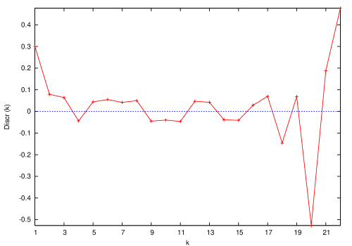
Figure 1: Discrepancy Discr, as predicted by (5.11), vs wavenumber $k$ for data obtained by spectral simulation in double precision; rounding noise becomes significant beyond wavenumber 17.

It is seen that the discrepancy falls to about 3.5% of the nominal value $1/\ln 2$ before getting swamped by rounding noise around wavenumber 17.

It is actually possible to significantly decrease the discrepancy by using a better processing of the numerical output, called asymptotic extrapolation, developed recently by van der Hoeven jorasint and which is related to the theory of transseries ecalle ; jorisspringer . The basic idea is to perform on the data a sequence of transformations which successively strip off the leading and subleading terms in the asymptotic expansion (here for large $|k|$). Eventually, the transformed data allow a very simple interpolation (mostly by a constant). The procedure can be carried out until the transformed data become swamped by rounding noise or display lack of asymptoticity, whichever occurs first. After the interpolation stage, the successive transformations are undone. This determines the asymptotic expansion of the data up to a certain order of subdominant terms. An elementary introduction to this method may be found in PF06 , from which we shall also borrow the notation for the various transformations: I for “inverse”, R for “ratio”, SR for “second ratio”, D for “difference” and Log for “logarithm”. The choice of the successive transformations is dictated by various tests which roughly allow to find into which broad asymptotic class the data and their transformed versions fall.

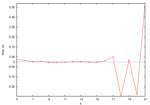
Figure 2: Discrepancy Discr vs wavenumber $k$ for the same data as in Fig. 1, but processed by a 5-stage asymptotic extrapolation method.

In the present case, the appropriate sequence of transformations is: Log, D, D, I, D. Because of the relatively low precision of the data it is not possible to perform more than five transformations, so that the method gives us access only to the leading-order asymptotic behavior, namely $|\hat{u}(k,1)|\simeq\mathrm{e}^{-C_{\star}|k|\ln|k|}$. It may be shown that the constant $C_{\star}=-1/u^{\rm(5)}$ where $u^{\rm(5)}$ is the constant value of the high-$|k|$ interpolation $u^{\rm(5)}(|k|)$ after the 5th stage of transformation. Fig. 2 shows the discrepancy $u^{\rm(5)}(|k|)+\ln 2$ . The absolute value of the discrepancy lingers around 0.002 to 0.005 before being swamped by rounding noise at wavenumber 17. Thus with asymptotic extrapolation the discrepancy does not exceed 0.7% of the nominal value $\ln 2$. The accuracy of the determination has thus improved by about a factor 5, compared to the naive method without asymptotic extrapolation.

To improve further on this result and get some indication as to the type of subdominant corrections present in the large-wavenumber expansion of the Fourier coefficients it would not suffice to increase the spatial resolution, since rounding noise would still swamp the signal beyond a wavenumber of roughly 17. Higher precision spectral calculations are doable but not very simple because high-precision fast Fourier transform packages are still in the experimental phase.

In the next Section we shall present an alternative method, significantly less versatile as to the choice of the initial condition because it exploits the algebraic structure of a certain special class of solutions, but which also allows to work easily in arbitrary precision and thus to make better use of asymptotic extrapolation for determining the constant $C_{\star}$.

5.3 Half-space (Fourier) supported initial conditions

So far we have limited ourselves to initial conditions that are real entire functions. Hence the Fourier coefficients had Hermitian symmetry: $\hat{u}_{0}(-k)=\hat{u}_{0}^{*}(k)$, where the star denotes complex conjugation. With complex initial data there are no analytical results when the dissipation is exponential, even when the initial conditions are entire because the energy conservation relation – now about a complex-valued quantity – ceases to give $L^{2}$-type bounds. Actually, as already pointed out, Li and Sinai LS07 showed that the 3D NSE can display finite-time blow up with suitable complex initial data. It is however straightforward to adapt to complex solutions the heuristic argument of Section 5.1 and to predict a high-wavenumber leading-order term exactly of the same form as for real solutions. This is of interest since we shall see that there is a class of periodic complex initial conditions for which, provided the Burgers equation is written in terms as the Fourier coefficients as in Sinai05 and LS07 , any given Fourier coefficient can be calculated at arbitrary times $t$ with a finite number of operations, most easily performed on a computer, by using either symbolic manipulations or arbitrary-high precision floating point calculations.

For the case of the Burgers equation, this class consists of initial conditions having the Fourier coefficients supported in the half line $k>0$. We shall refer to this class of initial data as “half-space (Fourier) supported”.

Because of the convolution structure of the nonlinearity when written in terms of Fourier coefficients, it is obvious that with an initial condition supported in the $k>0$ half line, the solution will also be supported in this half line. A similar idea has been used in three dimensions for studying the singularities for complex solutions of the 3D Euler equations caflisch .

Specifically, we consider again the 1D Burgers equation (5.1)-(5.2) with $2\pi$-periodic boundary conditions for $t\geq 0$, rewritten as (5.5), in terms of the Fourier coefficients $\hat{u}(k,t)$, assumed here to exist. The $k$-dependent real, even, non-negative dissipation coefficient $\mu\mathrm{e}^{G(k)}$ is denoted by $\rho(k)$. The initial conditions $\hat{u}_{0}(k)$ ($k=1,2,\ldots$) are chosen arbitrarily, real or complex. We then have the following Proposition, which is of purely algebraic nature:

Proposition 5.1    Eq. (5.5) with the initial conditions $\hat{u}(k,0)=0$ ($k\leq 0$) and $\hat{u}(k,0)=\hat{u}_{0}(k)$ ($k=1,2,\ldots$) defines, for all $k>0$ and $t>0$, $\hat{u}(k,t)$ as a polynomial functions of the set of $\hat{u}_{0}(p)$ with $0<p\leq k$.

Proof    From (5.5), after integration of the dissipative term, we obtain, for $k>0$ and $t>0$

$$\hat{u}(k,t)=\mathrm{e}^{-t\rho(k)}\hat{u}_{0}(k)-\frac{\mathrm{i}\,k}{2}\int_{0}^{t}ds\,\mathrm{e}^{-(t-s)\rho(k)}\sum_{p=1}^{k-1}\hat{u}(p,s)\hat{u}(k-p,s).$$ (5.12)

Observe that $\hat{u}(k,t)$, given by (5.12), involves $\hat{u}(k,0)$ (linearly) and the set of Fourier coefficients $\hat{u}(p,s)$ for $1\leq p\leq k-1$ and $0\leq s<t$ (quadratically). The proof follows by recursive use of this property for $k$, $k-1$, …, $1$.

Note that the solution can be obtained without any truncation error on a computer, using symbolic manipulation. Alternatively it can be calculated in arbitrary high-precision floating point arithmetic.

Now we specialize the initial condition even further, by assuming that the only Fourier harmonic present in the initial condition has $k=1$. We take

$$u_{0}(x)=\mathrm{i}\,{\cal A}\mathrm{e}^{\mathrm{i}\,x},$$ (5.13)

for which $\hat{u}_{0}(1)=\mathrm{i}\,{\cal A}$, while all the other coefficients vanish.

Setting, for $k>0$,

$$\hat{v}(k,t)\coloneqq\frac{\hat{u}(k,t)}{\mathrm{i}\,{\cal A}^{k}},$$ (5.14)

we obtain from (5.12) by working out the power series to the second order the following fully explicit expressions of the first two Fourier coefficient at any time $t>0$:

$$\hat{v}(1,t)=\mathrm{e}^{-\rho(1)t},\qquad\hat{v}(2,t)=\frac{\mathrm{e}^{-2\rho(1)t}}{\rho(2)-2\rho(1)}-\frac{\mathrm{e}^{-\rho(2)t}}{\rho(2)-2\rho(1)}.$$ (5.15)

For the one-mode initial condition with ${\cal A}=1$ and $\rho(k)=\mathrm{e}^{|k|}$ (exponential dissipation with $\mu=1$ and (${k_{\rm d}}=1$), we have calculated the Fourier coefficients $\hat{v}(k,1)$ for $k=1,2,\ldots,24$ using Maple symbolic calculation with a forty-digit accuracy.

The data have then been processed using asymptotic extrapolation as in Section 5.2 with the same five transformations Log, D, D, I, D.  Fig. 3 shows the discrepancy $\hat{v}^{\rm(5)}(k,1)+\ln 2$ between the 5th stage of interpolation and the prediction from the dominant balance argument. It is seen that the discrepancy drops to $-2.3\times 10^{-3}$. Thus the relative error is about $3\times 10^{-3}$. The oscillations in the discrepancy, if they continue to higher wavenumbers would indicate that the first subdominant correction to the asymptotic behavior of the Fourier coefficient $\mathrm{e}^{-(1/\ln 2)|{\tilde{k}}\ln|{\tilde{k}}|}$ is a prefactor involving a complex power of the wavenumber.

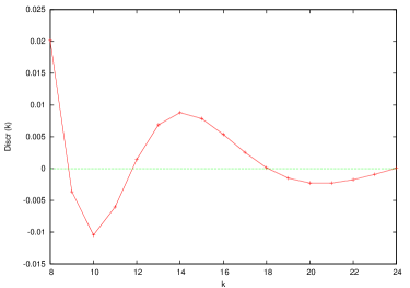
Figure 3: Fifth stage of asymptotic interpolation showing the discrepancy with respect to the heuristic prediction $C_{\star}=1/\ln 2$. Note the decaying oscillatory behavior.

Finally, we address the issue of what kind of solution we have constructed by this Fourier-based algebraic method. Is it a “classical” sufficiently smooth global-in-time solution of the Burgers equations (5.1)-(5.2) written in the physical space? We have here obtained strong numerical evidence that the Fourier coefficients decrease faster than exponentially with the wavenumber and thus define a classical solution which is an entire function of the space variable. This is however just a conjecture. The tools used in Section 2 to prove the entire character of the solution rely heavily on the definite positive character of the energy, a property lost with complex solutions.

6 Conclusions

In this paper we have proved that for a large class of evolution PDE’s, including the 3D NSE, exponential or faster-growing dissipation implies that the solution becomes and remains an entire function in the space variables at all times. Exponential growth constitutes a threshold: subexponential growth with a Fourier symbol $\mathrm{e}^{|k|^{\alpha}}$, where $0<\alpha<1$ makes the solution analytic (but not entire) as is the case in 2D (and generally conjectured in 3D). Furthermore, for the 3D NSE and the 1D Burgers equation with a dissipation having the Fourier symbol $\mu\mathrm{e}^{|k|/{k_{\rm d}}}$, we have shown that the amplitude of the Fourier coefficients is bounded by $\mathrm{e}^{-C|{\tilde{k}}|\ln|{\tilde{k}}|}$ (where ${\tilde{k}}\coloneqq k/{k_{\rm d}}$) for any $C<1/(2\ln 2)$. For the case of the 1D Burgers equation we have good evidence that this can be improved to $C<C_{\star}=1/\ln 2$ since the high-$|k|$ asymptotics seems to have a leading term precisely of the form $\mathrm{e}^{-C_{\star}|{\tilde{k}}|\ln|{\tilde{k}}|}$; the evidence comes both from a heuristic dominant balance argument and from high-precision simulations. The heuristic argument can actually be carried over somewhat loosely to the expNSE in any dimension: again the dominant nonlinear interaction contributing to wave vector $k$ comes from the wave vectors $p=q=k/2$; actually the condition of incompressibility kills nonlinear interactions between exactly parallel wave vectors but this is only expected to modify algebraic prefactors in front of the exponential term.

We thus conjecture that the $C_{\star}=1/\ln 2$ also holds for expNSE in any space dimension $d\geq 2$. Of course there is a substantial gap between the bound and the conjectured asymptotic behavior. It seems that such a gap is hard to avoid when using $L^{2}$-type norms. For proving the entire character of the solution such norms were appropriate. Beyond this, it is appears more advisable to try bounding directly the moduli of Fourier coefficients by using the power series method LS07 ; Sinai05 . A first step in this direction would be to prove that $C_{\star}=1/\ln 2$ for initial conditions whose Fourier coefficients are compactly supported in a product of half-spaces, of the kind considered in Section 5.3.

Exponential dissipation differs from ordinary dissipation (with a Laplacian or a power thereof) not only by giving a faster decay of the Fourier coefficients but by doing so in a universal way: with ordinary dissipation the decay of the Fourier coefficient is generally conjectured to be, to leading order, of the form $\mathrm{e}^{-\eta|k|}$ where $\eta$ depends on the viscosity $\nu$ and on the energy input or on the size of the initial velocity; with exponential dissipation the decay is $\mathrm{e}^{-C_{\star}|{\tilde{k}}|\ln|{\tilde{k}}|}$ where $C_{\star}=1/\ln 2$ and thus depends neither on the coefficient $\mu$ which plays the role of the viscosity nor on the initial data. As a consequence, it is expected that exponential dissipation will not exhibit the phenomenon of dissipation-range intermittency, which for the usual dissipation can be traced back either to the fluctuations of $\eta$ rhk67 or to complex singularities of a velocity field that is analytic but not entire frischmorf .

Finally some comments on the practical relevance of modified dissipation. First, let us comment on “hyperviscosity”, the replacement of the (negative) Laplacian by its power of order $\alpha>1$. Of course we know that specialists of PDE’s have traditionally been interested in the hyperviscous 3D NSE, perhaps to overcome the frustration of not being able to prove much about the ordinary 3D NSE. But scientists doing numerical simulations of the NSE, say, for engineering, astrophysical or geophysical applications, have also been using hyperviscosity because it is often believed to allow effectively higher Reynolds numbers without the need to increase spatial resolution. Recently, three of us (UF, WP, SSR) and other coauthors have shown that when using a high power $\alpha$ of the Laplacian in the dissipative term for 3D NSE or 1D Burgers, one comes very close to a Galerkin truncation of Euler or inviscid Burgers, respectively FKPPRWZ08 . This produces a range of nearly thermalized modes which shows up in large-Reynolds number spectral simulations as a huge bottleneck in the Fourier amplitudes between the inertial range and the far dissipation range. Since the bottleneck generates a fairly large eddy viscosity, the hyperviscosity procedure with large $\alpha$ actually decreases the effective Reynolds number.

Next, consider exponential dissipation. In 1996 Achim Wirth noticed that when used in the 1D Burgers equation, cosh dissipation produces almost no bottleneck although it grows much faster than a power of the wavenumber at high wavenumbers AW . It is now clear that such a dissipation will produce a faster-than-exponential decay at the highest wavenumbers. But at wavenumbers such that $|k|\ll{k_{\rm d}}$ a dissipation rate $-\mu(1-\cosh k/{k_{\rm d}})$ reduces to $\mu|k|^{2}/(2{k_{\rm d}}^{2})$, to leading order, which is the ordinary (Laplacian) dissipation. With the ordinary 1D Burgers equation it may be shown analytically that there is no bottleneck. For the ordinary 3D NSE, experimental and numerical results show the presence of a rather modest bottleneck (for example the “compensated” three-dimensional energy spectrum $|k|^{+5/3}E(|k|)$ overshoots by about 20%.). If in a simulation with cosh dissipation $\mu$ and ${k_{\rm d}}$ are adjusted in such a way that dissipation starts acting at wavenumbers slighter smaller than ${k_{\rm d}}$, the beginning of the dissipation range will be mostly as with an ordinary Laplacian, that is with no or little bottleneck. At higher wavenumbers, where the exponential growth of the dissipation rate is felt, faster than exponential decay will be observed. In principle this can be used to avoid wasting resolution without developing a serious bottleneck. Faster than exponentially growing dissipation, e.g. $\mu\left(\mathrm{e}^{(|k|/{k_{\rm d}})^{2}}-1\right)$, may be even better because the prediction is that the Fourier coefficients will display Gaussian decay. Testing the advantages and drawbacks of different types of faster-than-algebraically growing dissipations for numerical simulations is left for future work.

We thank J.-Z. Zhu and A. Wirth for important input and M. Blank, K. Khanin, B. Khesin and V. Zheligovsky for many remarks. CB acknowledges the warm hospitality of the Weizmann Institute and SSR that of the Observatoire de la Côte d’Azur, places where parts of this work were carried out. The work of EST was supported in part by the NSF grant No. DMS-0708832 and the ISF grant No. 120/06 . SSR thanks R.  Pandit, D. Mitra and P. Perlekar for useful discussions and acknowledges DST and UGC (India) for support and SERC (IISc) for computational resources. UF, WP and SSR were partially supported by ANR “OTARIE” BLAN07-2_183172 and used the Mésocentre de calcul of the Observatoire de la Côte d’Azur for computations.

References

- (1) Majda, A.J., Bertozzi, A.L.: Vorticity and Incompressible Flow. Cambridge Texts in Applied Mathematics, Cambridge: Cambridge University Press, 2001.
- (2) Frisch, U., Matsumoto, T., Bec, J.: Singularities of Euler flow? Not out of the blue! J. Stat. Phys. 113 , 761–781 (2003).
- (3) Bardos, C., Titi, E.S.: Euler equations of incompressible ideal fluids. Uspekhi Mat. Nauk 62, 5–46 (2007). English version Russian Math. Surv. 62, 409–451 (2007).
- (4) Constantin, P.: On the Euler equations of incompressible fluids. Bull. Amer. Math. Soc. 44, 603–621 (2007).
- (5) Eyink, G., Frisch, U., Moreau, R., Sobolevskiĭ, A.: Proceedings of “Euler Equations: 250 Years On”, Aussois, June 18–23, 2007. Physica D 237, no. 14–17 (2008).
- (6) Lions, J.L.: Quelques Méthodes de Résolution des Problèmes aux Limites non Linéaires. Paris: Gauthier-Villars, 1969.
- (7) Constantin, P.; Foias, C.: Navier-Stokes equations. Chicago Lectures in Mathematics. Chicago: University of Chicago Press, 1988.
- (8) Fefferman, C.: Existence & smoothness of the Navier–Stokes equation. Millenium problems of the Clay Mathematics Institute (2000). Available at www.claymath.org/millennium/Navier-Stokes_Equations/Official_Problem_Description.pdf.
- (9) Temam, R.: Navier-Stokes equations. Theory and numerical analysis. Revised edition. With an appendix by F. Thomasset. Published by AMS Bookstore, 2001.
- (10) Sohr, H.: The Navier-Stokes equations. Basel: Birkhäuser, 2001.
- (11) Brachet, M.-E., Meiron, D.I., Orszag, S.A., Nickel, B.G., Morf, R.H., Frisch, U.: Small-scale structure of the Taylor-Green vortex, J. Fluid Mech. 130, 411–452 (1983).
- (12) Neumann, J. von.: Recent theories of turbulence (1949). In: Collected works (1949–1963) 6, 37–472, ed. A.H. Taub. New York: Pergamon Press, 1963.
- (13) Li, D., Sinai, Ya. G.: Blow-ups of complex solutions of the 3D Navier–Stokes system and renormalization group method. J. Eur. Math. Soc. 10, 267–313 (2008).
- (14) Oliver, M., Titi, E.S.: On the domain of analyticity for solutions of second order analytic nonlinear differential equations. J. Differ. Equations 174, 55–74 (2001).
- (15) Pauls, W., Matsumoto, T.: Lagrangian singularities of steady two-dimensional flow. Geophys. Astrophys. Fluid. Dyn. 99, 61–75 (2005).
- (16) Senouf, D., Caflisch, R., Ercolani, N.: Pole dynamics and oscillation for the complex Burgers equation in the small-dispersion limit. Nonlinearity 9, 1671–1702 (1996).
- (17) Poláčik, P., Šverák, V.: Zeros of complex caloric functions and singularities of complex viscous Burgers equation. Preprint. 2008. arXiv:math/0612506v1 [math.AP].
- (18) Ladyzhenskaya, O.A.: The Mathematical Theory of Viscous Incompressible Flow (1st ed.). New York: Gordon and Breach, 1963.
- (19) Holloway, G.: Representing topographic stress for large-scale ocean models. J. Phys. Oceanogr. 22, 1033–1046 (1992).
- (20) Foias, C., Temam, R.: Gevrey class regularity for the solutions of the Navier–Stokes equations. J. Funct. Anal. 87, 359–369 (1989).
- (21) Ferrari, A., Titi, E.S.: Gevrey regularity for nonlinear analytic parabolic equations. Commun. Part. Diff. Eq. 23, 1–16 (1998).
- (22) Agmon, S.: Lectures on Elliptic Boundary Value Problems. Mathematical Studies, Van Nostrand, 1965.
- (23) Cao, C., Rammaha, M., Titi, E.S.: The Navier–Stokes equations on the rotating sphere: Gevrey regularity and asymptotic degrees of freedom. Zeitschrift für Angewandte Mathematik und Physik (ZAMP) 50, 341–360 (1999).
- (24) Doelman, A., Titi, E.S.: Regularity of solutions and the convergence of the Galerkin method in the Ginzburg–Landau equation, Numerical Functional Analysis and Optimization 14, 299–321 (1993).
- (25) Masuda, K.: On the analyticity and the unique continuation theorem for solutions of the Navier–Stokes equation. Proc. Japan Acad. 43, 827–832 (1967).
- (26) Doering, C.R., Titi, E.S.: Exponential decay rate of the power spectrum for solutions of the Navier–Stokes equations. Phys. Fluids 7, 1384–1390 (1995).
- (27) Gottlieb, D., Orszag, S.A.: Numerical Analysis of Spectral Methods. Philadelphia: SIAM, 1977.
- (28) Frisch, U., She, Z.S., Thual, O.: Viscoelastic behaviour of cellular solutions to the Kuramoto-Sivashinsky model. J. Fluid Mech. 168, 221–240 (1986).
- (29) Cox, C.M., Matthews, P.C.: Exponential time differencing for stiff systems. J. Comput. Phys. 76, 430–455 (2002).
- (30) van der Hoeven, J.: On asymptotic extrapolation. J. Symbolic Computation 44, 1000–1016 (2009); see also http://www.texmacs.org/joris/extrapolate/extrapolate-abs.html
- (31) Ecalle, J.: Introduction aux Fonctions Analysables et Preuve Constructive de la Conjecture de Dulac. Actualités mathématiques. Paris: Hermann, 1992.
- (32) van der Hoeven, J.: Transseries and Real Differential Algebra. Lecture Notes in Math. 1888, Berlin: Springer, 2006.
- (33) Pauls, W., Frisch, U.: A Borel transform method for locating singularities of Taylor and Fourier series, J. Stat. Phys. 127, 1095–1119 (2007). arXiv:nlin/0609025v2 [nlin.CD]
- (34) Sinai, Ya. G.: Diagrammatic approach to the 3D Navier-Stokes system. Russ. Math. Surv. 60, 849–873 (2005).
- (35) Caflisch, R.E.: Singularity formation for complex solutions of the 3D incompressible Euler equations. Physica D 67, 1–18 (1993).
- (36) Kraichnan, R.H.: Intermittency in the very small scales of turbulence. Phys. Fluids 10, 2080–2082 (1967).
- (37) Frisch, U., Morf, R.: Intermittency in nonlinear dynamics and singularities at complex times. Phys. Rev. A 10, 2673–2705 (1981).
- (38) Frisch, U., Kurien, S., Pandit, R., Pauls, W., Ray, S.S., Wirth, A., Zhu, J.-Z.: Hyperviscosity, Galerkin truncation and bottlenecks in turbulence, Phys. Rev. Lett. 101, 144501 (2008). arxiv:0803.4269 [nlin.CD].
- (39) Wirth, A. Private communication (1996).
- (40) Zhu, J.-Z. Private communication (2008).
- (41) Orszag, S.A. Private communication (1979).