Collective dynamical response of coupled oscillators with any network structure

Abstract

We formulate a reduction theory that describes the response of an oscillator network as a whole to external forcing applied nonuniformly to its constituent oscillators. The phase description of multiple oscillator networks coupled weakly is also developed. General formulae for the collective phase sensitivity and the effective phase coupling between the oscillator networks are found. Our theory is applicable to a wide variety of oscillator networks undergoing frequency synchronization. Any network structure can systematically be treated. A few examples are given to illustrate our theory.

An assembly of coupled limit-cycle oscillators often behaves like a single large oscillator. This general scenario recurs in a wide variety of rhythmic phenomena in living organisms, ranging from circadian oscillations, cardiac rhythms to pathological phenomena such as epilepsy and Parkinsonian disease Winfree (1980); Kuramoto (1984); Tass (1999); Pikovsky et al. (2001); Reppert and Weaver (2002). Recent experiments using electrochemical oscillators simulate such naturally arising populations of oscillators in an idealized form Kiss et al. (2002).

Many previous studies have been devoted to answering how and under what conditions oscillators mutually synchronize. In comparison, little attention has been paid to investigating the dynamical response of an oscillator network to external stimuli. Such an inquiry would shed light on mechanisms underlying biological functions (such as the phase response curves of circadian rhythms Johnson (1999)), external control, and inter-network synchronization of oscillator networks Okuda and Kuramoto (1991). Establishing a description of the collective dynamics on the basis of “microscopic” knowledge, i.e., the nature of the constituent oscillators and their mutual coupling, presents a challenging task from a theoretical point of view. In particular, it would be ideal if the collective dynamics could be described in terms of a single, suitably defined collective phase $\Theta$ in a closed form. A quantity of central importance will then be the phase sensitivity of a population as a whole to external weak stimuli . This function has already been derived Kawamura et al. (2008) for a system consisiting of a large assembly of identical phase oscillators with global coupling, with each oscillator being driven independently by random time-dependent noise.

In this Letter, we argue that there is yet another general situation for which a similar phase description can be formulated. In contrast to Ref. Kawamura et al., 2008, we consider noise-free but nonidentical oscillators undergoing full frequency synchronization (in which all the oscillators have exactly the same frequency due to coupling). A similar situation has also been studied by Ko and Ermentrout for two symmetrically coupled and globally coupled oscillators very recently Ko and Ermentrout (2008). A distinct advantage of our present approach is that it may deal with any system size, any connectivity, any heterogeneous coupling, and nonuniform external forcing. Moreover, the theory is extended to include multiple populations simply by reinterpreting the external stimuli applied to a given population as the coupling forces originating from the other populations, which enables us to predict the synchronization behavior between oscillator networks. General formulae for the collective phase sensitivity and the effective phase coupling between the oscillator networks are found.

Consider a network of $N$ coupled limit-cycle oscillators under external forcing. The forcing is generally nonuniform, i.e., individual oscillators receive different inputs. As is well known Kuramoto (1984), if the heterogeneity of oscillators, the coupling between oscillators, and external forcing are weak, the system is describable by the phase equation

$$\dot{\phi}_{i}=\omega_{i}+\sum_{j=1}^{N}\Gamma_{ij}(\phi_{i}-\phi_{j})+\epsilon Z(\phi_{i})\xi_{i}(t).$$ (1)

Here $\phi_{i}$ is the phase of the $i$th oscillator ($i=1,\ldots,N$), $\omega_{i}$ its natural frequency, and $\Gamma_{ij}$ the coupling force from the $j$th oscillator to the $i$th oscillator. The terms $\xi_{i}(t)$ and $Z(\phi_{i})$ respectively represent the time-dependent external force and the phase sensitivity of the oscillator $i$ to external perturbation . Parameter $\epsilon$ is the characteristic intensity of the external forcing.

Our aim is to establish the collective phase description for Eq. (1), i.e. to derive the dynamical equation for a suitably defined macroscopic variable that describes the response to external forcing. This is generally formulated under two basic assumptions. (i) In the absence of external forcing a stable periodic solution corresponding to a fully frequency-synchronized state exists, and thus, the oscillator network behaves as a single large limit-cycle oscillator. (ii) The external force is even weaker than the coupling force, i.e. $\epsilon\ll 1$, so that the synchronized state is almost unaltered under external forcing. Under these assumptions, the phase reduction method Kuramoto (1984) applicable to a weakly perturbed oscillator can be applied (once again) to the oscillator network by interpreting the unperturbed system as a single limit-cycle oscillator.

For convenience, we begin by rewriting Eq. (1) in terms of the $N$-dimensional state vector $\bm{X}=(\phi_{1},\phi_{2},\ldots,\phi_{N})$ as

$$\dot{\bm{X}}={\bm{F}}({\bm{X}})+\epsilon{\bm{p}}({\bm{X}},t),$$ (2)

where $F_{i}(\bm{X})=\omega_{i}+\sum_{j=1}^{N}\Gamma_{ij}(\phi_{i}-\phi_{j})$ and $p_{i}(\bm{X},t)=Z(\phi_{i})\xi_{i}(t)$. A frequency synchronized state (or, more exactly, a phase locked state) for $\epsilon=0$ is found as a solution of $F_{i}(\bm{X})=\Omega$ for all $i$. This “limit-cycle” solution is denoted by

$$\bm{X}_{0}(\Theta)=(\Theta+\phi_{1}^{0},\Theta+\phi_{2}^{0},\ldots,\Theta+\phi_{N}^{0}),\ \Theta=\Omega t,$$ (3)

where $\phi_{i}^{0}$ is constant. We then extend the definition of $\Theta$ outside the limit-cycle orbit as a scalar field $\Theta(\bm{X})$. The identity $\dot{\Theta}=(d\Theta/d\bm{X})\cdot(d\bm{X}/dt)$ implies

$$\dot{\Theta}=\frac{d\Theta}{d\bm{X}}\cdot\left\{\bm{F}(\bm{X})+\epsilon\bm{p}(\bm{X},t)\right\}.$$ (4)

As is usually done in the phase reduction process, we now adopt the definition of $\Theta(\bm{X})$ such that in the absence of the forcing, $\dot{\Theta}=\Omega$ is identically satisfied, i.e., $(d\Theta/d\bm{X})\cdot\bm{F}(\bm{X})=\Omega$. We call $\Theta(\bm{X})$ the collective phase . Due to the assumption of weak forcing, $(d\Theta/d\bm{X})\cdot\bm{p}(\bm{X},t)$ may be evaluated at $\bm{X}=\bm{X}_{0}(\Theta)$. Then, to the lowest order in $\epsilon$ Eq. (4) becomes

$$\dot{\Theta}=\Omega+\epsilon\frac{d\Theta}{d\bm{X}_{0}}\cdot\bm{p}(\bm{X}_{0},t).$$ (5)

Let the linearized equation of $(\ref{X-eq})$ with $\epsilon=0$ be $\dot{\bm{Y}}=L\bm{Y}$, where $\bm{Y}$ is the deviation defined by $\bm{Y}=\bm{X}-\bm{X}_{0}$. Due to the symmetry of $\bm{F}(\bm{X})$, the Jacobian $L$ is a constant matrix, one eigenvalue of which equals zero with the corresponding eigenvector given by $\bm{U}=d\bm{X}_{0}(\Theta)/d\Theta=(1,1,\ldots,1)$. We define row vector $\bm{U}^{*}$ as the left zero-eigenvector of $L$, i.e., $\bm{U}^{*}L=0$, with the normalization condition $\bm{U}^{*}\bm{U}$=1, or, $\sum_{i=1}^{N}U_{i}^{\ast}=1$. It can then be argued that $d\Theta/d\bm{X}_{0}$ becomes identical to $\bm{U}^{*}$ Kuramoto (1984). Thus, Eq. (5) takes the form

$$\dot{\Theta}=\Omega+\epsilon\bm{\zeta}(\Theta)\cdot\bm{\xi}(t),$$ (6)

where $\bm{\xi}=(\xi_{1},\xi_{2},\ldots,\xi_{N})$ and $\bm{\zeta}(\Theta)$, which is interpreted as the collective phase sensitivity, is a vector with components

$$\zeta_{i}(\Theta)=U_{i}^{*}Z(\Theta+\phi_{i}^{0}).$$ (7)

Equations (6) and (7) have clarified the response of the collective mode of the synchronized network. There, the forcing to the oscillator $i$ has turned out to be weighted by $U_{i}^{*}$. We thus call $\bm{U}^{*}$ the weight vector henceforth.

In what follows, we often consider uniform external forcing, $\xi_{i}(t)=\xi(t)$ for all $i$. In such a case, Eq. (6) is further reduced to $\dot{\Theta}=\Omega+\epsilon\zeta(\Theta)\xi(t)$, where $\zeta(\Theta)$ is the collective phase sensitivity defined for uniform forcing, $\zeta(\Theta)=\sum_{i=1}^{N}U_{i}^{*}Z(\Theta+\phi_{i}^{0})$. Generally speaking, $\zeta(\Theta)$ deviates from $Z(\phi)$ more significantly as the phases of the constituent oscillators are more widely distributed.

An analytic formula of weight vector $\bm{U}^{*}$ is given as follows. The elements of $L$ are given by

$$L_{ij}=\delta_{ij}\sum_{k\neq i}^{N}\Gamma_{ik}^{\prime}\left(\phi_{i}^{0}-\phi_{k}^{0}\right)-(1-\delta_{ij})\Gamma_{ij}^{\prime}\left(\phi_{i}^{0}-\phi_{j}^{0}\right).$$ (8)

Note that the relation $L\bm{U}=\sum_{j=1}^{N}L_{ij}=0$ holds. We define the $(i,i)$-cofactor of $L$ as $M_{i}={\rm det}\,L(i,i)$, which is the determinant of the submatrix $L(i,i)$, that is $L$ with the $i$-th row and column removed. One can prove that, for any $L$ with $\sum_{j=1}^{N}L_{ij}=0$, the row vector $(M_{1},M_{2},...,M_{N})$ is a left zero-eigenvector of $L$, i.e., $\sum_{j=1}^{N}M_{j}L_{ji}=0$ Biggs (1997). Using the normalization condition, we obtain the algebraic expression of $\bm{U}^{*}$ as

$$\bm{U}^{*}=(M_{1},M_{2},\ldots,M_{N})/M,$$ (9)

where $M=\sum_{i=1}^{N}M_{i}$. This expression is valid for any network structure. Note that, for networks with both bidirectional connection patterns and symmetric coupling functions, $L$ is symmetric and $U_{i}^{*}$ is trivially $1/N$ for all $i$, which is the case even for networks with strongly heterogeneous connectivity including scale-free networks. In many cases, however, $L$ is asymmetric and $\bm{U}^{*}$ is heterogeneous.

Next, we formulate the collective phase description of multiple networks of phase oscillators. We are concerned with the case in which external forcing is absent, while $\epsilon\xi_{i}(t)$ in the last term in Eq. (1) is interpreted as representing the coupling force coming from oscillators of other networks. For clarity, we consider a simple system in which two identical networks composed of $N$ oscillators, called group A and group B, are uniformly coupled (the extension to a more general case, e.g., weakly heterogeneous multiple groups, is straightforward). The dynamical equations of the system are given by

$$\dot{\phi}_{i}^{\rm A} =\omega_{i}+\sum_{j=1}^{N}\Gamma_{ij}(\phi_{i}^{\rm A}-\phi_{j}^{\rm A})+\epsilon Z(\phi_{i}^{\rm A})\xi(\{\phi^{\rm B}_{k}\}),$$ (10)

$$\dot{\phi}_{i}^{\rm B} =\omega_{i}+\sum_{j=1}^{N}\Gamma_{ij}(\phi_{i}^{\rm B}-\phi_{j}^{\rm B})+\epsilon Z(\phi_{i}^{\rm B})\xi(\{\phi^{\rm A}_{k}\}),$$

where $\phi_{i}^{\rm X}$ is the phase of the oscillator $i$ in group X (X=A, B), and $\xi(\{\phi^{\rm X}_{k}\})$ denotes a function of $\phi_{1}^{\rm X},\phi_{2}^{\rm X},\ldots,\phi_{N}^{\rm X}$, which represents the uniform coupling force coming from group X. Denoting the collective phases of the respective groups by $\Theta_{\rm A}$ and $\Theta_{\rm B}$, we obtain the resulting phase equation in the form

$$\dot{\Theta}_{\rm A} =\Omega+\epsilon\zeta(\Theta_{\rm A})\xi(\{\Theta_{\rm B}+\phi_{k}^{0}\}),$$ (11)

$$\dot{\Theta}_{\rm B} =\Omega+\epsilon\zeta(\Theta_{\rm B})\xi(\{\Theta_{\rm A}+\phi_{k}^{0}\}).$$

Noting that the dominant time-dependence of $\Theta_{\rm A,B}$ is $\Omega t$, we may obtain the effective coupling $\gamma(\Theta_{\rm A}-\Theta_{\rm B})$ between the groups by time-averaging of Eq. (11) over the common period $2\pi/\Omega$. Putting $\Theta_{\rm A,B}=\Omega t+\theta_{\rm A,B}$, we perform the averaging as

$$\gamma (\Theta_{\rm A}-\Theta_{\rm B})=\gamma(\theta_{\rm A}-\theta_{\rm B})=$$

$$\frac{1}{2\pi}\int_{0}^{2\pi}d(\Omega t)\zeta(\Omega t+\theta_{\rm A})\xi(\{\Omega t+\theta_{\rm B}+\phi_{k}^{0}\}),$$ (12)

where $\gamma$ rather than $\Gamma$ has been used to indicate that this coupling function acts between the groups. In this way, we succeeded in deriving the collective phase equation in the simple form

$$\dot{\Theta}_{\rm A} =\Omega+\epsilon\gamma(\Theta_{\rm A}-\Theta_{\rm B}),$$ (13)

$$\dot{\Theta}_{\rm B} =\Omega+\epsilon\gamma(\Theta_{\rm B}-\Theta_{\rm A}).$$

We give two examples to illustrate our theory.

Example I: the dependence of weight vector $\bm{U}^{*}$ on the connectivity. We consider a network of identical oscillators with homogeneous coupling, i.e., $\omega_{i}=\omega$ and $\Gamma_{ij}(\Delta\phi)=A_{ij}\Gamma(\Delta\phi)$ undergoing perfect phase synchrony. Here, $A$ is the adjacency matrix describing the connectivity, which is generally asymmetric and weighted. In such a system, the weight vector depends solely on the network architecture. By rescaling $t$ and $\epsilon$, we put $\Gamma^{\prime}(0)=-1$ without loss of generality. In perfect phase synchrony, i.e., $\phi_{i}^{0}=\phi^{0}$ for all $i$, $L$ is a Laplacian matrix generalized for asymmetric and weighted networks, given by $L_{ij}=-A_{ij}$ for $i\neq j$ and $L_{ii}=\sum_{j\neq i}^{N}A_{ij}$. We consider two small networks in which the weight vector $\bm{U}^{*}$ is easily calculated via the algebraic expression, Eq. (9). Figure 1(a) is a weighted network, where the weight vector is found to be a simple reflection of the connection weights. Figure 1(b) is a non-weighted network but its adjacency matrix is asymmetric. It is worth noticing that oscillator 2 is more influential than oscillator 3, although they have locally the same topological properties: one inward and two outward connections. In general, the weight vector depends on the global topology.

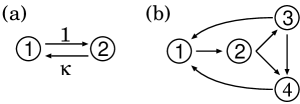
Figure 1: Examples of weight vector $\bm{U}^{*}$. Using Eq. (9), we find (a) $U^{*}_{1}:U^{*}_{2}=1:\kappa$ and (b) $U^{*}_{1}:U^{*}_{2}:U^{*}_{3}:U^{*}_{4}=2:4:3:1$.

Example II: collective phase sensitivity and group synchronization in limit-cycle oscillators. We illustrate that the collective phase sensitivity of a group of coupled oscillators varies with intra-group coupling strength. We then consider two groups of coupled oscillators with an additional inter-group coupling of fixed strength, and show that a nontrivial qualitative change in the synchronization behavior between the groups occurs when the individual collective phase sensitivities changes as a result of modifications to the intra-group coupling strength.

As schematically illustrated in Fig. 2(a), we consider the system in which a pair of identical groups A and B, each of which consists of two coupled limit-cycle oscillators, are mutually coupled. We use the Hindmarsh-Rose model as the limit-cycle oscillator, a model originally proposed as a neural model. The system reads

$$\dot{x}_{i}=3x_{i}^{2}-x_{i}^{3}+y_{i}-\mu_{i}+\sum_{j=1}^{4}D_{ij}x_{j},\,\,\dot{y}_{i}=1-5x_{i}^{2}-y_{i}.$$ (14)

Here, the coupling matrix $D$ is given as $D_{12,21,34,43}=K,D_{11,22,33,44}=-K,D_{13,23,31,41}=\epsilon$ with $K$ and $\epsilon$ being the coupling intensities for intra- and inter-groups, respectively. We assume $1\gg K\gg\epsilon=1.0\times 10^{-5}$. We set $\mu_{1}=\mu_{3}=-3.000$ and $\mu_{2}=\mu_{4}=-3.001$, corresponding to $\omega_{1,3}\simeq 1.80476,\omega_{2,4}\simeq 1.80443$, and thus $\Delta\omega\simeq 3.3\times 10^{-4}$. The wave form $x(\phi)$ and the phase sensitivity $Z(\phi)$ of an isolated oscillator obtained numerically are shown in Figs. 2(b) and 2(c), respectively.

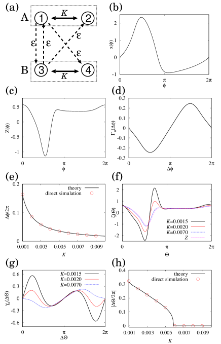
Figure 2: (color online) Results for a network of limit-cycle oscillators. (a) Network structure under consideration. (b) Waveform $x(\phi)$ and (c) phase sensitivity $Z(\phi)$ of an individual oscillator. (d) Antisymmetric part of the coupling function, $\Gamma_{\rm a}(\Delta\phi)$. (e) Phase difference $\Delta\phi^{0}$ between oscillators in each group. (f) Collective phase sensitivity $\zeta(\Theta)$ defined for uniform forcing. For $K=0.007,0.002,0.0015$, $(U_{1}^{*},U_{2}^{*})$ is respectively about $(1.35,-0.35),(2.87,-1.87)$ and $(2.89,-1.89)$. (g) Antisymmetric part of the collective coupling function, $\gamma_{\rm a}(\Delta\Theta)$. (h) Phase difference $\Delta\Theta$ between the groups.

The corresponding phase model is given by Eq. (10), where $\Gamma_{ij}(\Delta\phi)=K\Gamma(\Delta\phi)$, $\xi(\{\phi_{k}^{\rm A}\})=x(\phi_{1})$, and $\xi(\{\phi_{k}^{\rm B}\})=x(\phi_{3})$. From the phase reduction theory, the coupling function is calculated as $\Gamma(\phi_{1}-\phi_{2})=\frac{1}{2\pi}\int_{0}^{2\pi}d(\omega t)Z(\phi_{1}+\omega t)\{x(\phi_{2}+\omega t)-x(\phi_{1}+\omega t)\}$. For convenience, we display $\Gamma_{\rm a}(\Delta\phi)\equiv\Gamma(\Delta\phi)-\Gamma(-\Delta\phi)$ in Fig. 2(d). The phase difference $\Delta\phi^{0}$ between the oscillators $1$ and $2$ of a synchronized state is found as a stable solution of $\dot{\phi}_{1}=\dot{\phi}_{2}$ (where $\epsilon=0$ is assumed), and thus, a solution of $\Gamma_{\rm a}(\Delta\phi^{0})=\Delta\omega/K$. The predicted phase difference is plotted in Fig. 2(e) as a curve. It agrees well with numerical data obtained through direct numerical integration of Eq. (14). Using $Z(\phi)$, $\Delta\phi^{0}$, $\Gamma(\Delta\phi)$, and its derivative $\Gamma^{\prime}(\Delta\phi)$ obtained numerically, we can calculate $U_{1}^{*},U_{2}^{*}$, and $\zeta(\Theta)$. The results are shown in Fig. 2(f) and its caption. For large $K$ (compared to $\Delta\omega$), $\zeta(\Theta)$ is indistinguishable from $Z(\phi)$. As $K$ decreases, $\Delta\phi^{0}$ becomes larger, resulting in considerable variation in $\zeta(\Theta)$.

Given $\zeta(\Theta)$, the synchronization behavior between groups is now predicted. The collective coupling function $\gamma(\Delta\Theta)$ is calculated from Eq. (12) where $\xi(\phi)=x(\phi)$ in the system under consideration. For convenience, we display the antisymmetric part of $\gamma(\Delta\Theta)$ in Fig. 2(g). Putting $\dot{\Theta}_{\rm A}=\dot{\Theta}_{\rm B}$, we find the stable phase locking solution between groups, $\Delta\Theta\equiv\Theta_{\rm A}-\Theta_{\rm B}$. Predicted $\Delta\Theta$ is exhibited by the curve in Fig. 2(h), implying that the in-phase solution becomes unstable at around $K=0.006$ (via a pitch-fork bifurcation) and the out-of-phase solution appears below. Phase difference $\Delta\Theta$ (or equivalently, $\phi_{1}-\phi_{3}$) obtained from direct numerical integration of Eq. (14) is plotted in Fig. 2(h), which convinces us of the precision of the phase description.

In summary, we have formulated the response of the collective phase to weak external forcing given to constituent oscillators and the phase description for interacting oscillator networks. The present theory is valid for a wide class of weakly coupled oscillator networks undergoing full frequency synchronization, and thus, a broad applicability would be expected.

References

- Winfree (1980) A. T. Winfree, The Geometry of Biological Time (Springer, New York, 1980).
- Kuramoto (1984) Y. Kuramoto, Chemical Oscillations, Waves, and Turbulence (Springer, New York, 1984).
- Tass (1999) P. A. Tass, Phase Resetting in Medicine and Biology (Springer, Berlin, 1999).
- Pikovsky et al. (2001) A. Pikovsky, M. Rosenblum, and J. Kurths, Synchronization (Cambridge University Press, Cambridge, 2001).
- Reppert and Weaver (2002) S. M. Reppert and D. R. Weaver, Nature 418, 935 (2002).
- Kiss et al. (2002) I. Z. Kiss, Y. M. Zhai, and J. L. Hudson, Science 296, 5573 (2002); I. Z. Kiss, C. G. Rusin, H. Kori, and J. L. Hudson, Science 316, 1886 (2007); H. Kori, C. G. Rusin, I. Z. Kiss, and J. L. Hudson, Chaos 18, 026111 (2008).
- Johnson (1999) C. H. Johnson, Chronobiology international 16, 711 (1999).
- Okuda and Kuramoto (1991) K. Okuda and Y. Kuramoto, Prog. Theor. Phys. 86, 1159 (1991); E. Montbrio, J. Kurths, and B. Blasius, Phys. Rev. E 70, 056125 (2004); I. Z. Kiss, M. Quigg, S.-H. C. Chun, H. Kori, and J. L. Hudson, Biophysical Journal 94, 1121 (2008); J. H. Sheeba, A. Stefanovska, and P. V. E. McClintock, Biophysical Journal 95, 2722 (2008); E. Ott and T. M. Antonsen, Chaos 18, 037113 (2008); E. Barreto, B. Hunt, E. Ott, and P. So, Phys. Rev. E 77, 036107 (2008).
- Kawamura et al. (2008) Y. Kawamura, H. Nakao, K. Arai, H. Kori, and Y. Kuramoto, Phys. Rev. Lett. 101, 024101 (2008).
- Ko and Ermentrout (2008) T.-W. Ko and G. B. Ermentrout, arXiv/0809.3371.
- Biggs (1997) N. Biggs, Bulletin of the London Mathematical Society 29, 641 (1997).
- Winfree (1967) A. T. Winfree, J. Theor. Biol. 16, 15 (1967).
- Izhikevich (2007) E. M. Izhikevich, Dynamical Systems in Neuroscience (MIT Press, Cambridge, 2007).