A kinetic scheme for pressurised flows in non uniform closed water pipes

Abstract

The aim of this paper is to present a kinetic numerical scheme for the computations of transient pressurised flows in closed water pipe with non uniform sections. Firstly, we detail the derivation of the mathematical model in curvilinear coordinates and we performe a formal asymptotic analysis. The obtained system is written as a conservative hyperbolic partial differential system of equations. We obtain a kinetic interpretation of this system and we build the corresponding kinetic scheme based on an upwinding of the source terms written as the gradient of a “pseudo altitude”. The validation is lastly performed in the case of a water hammer in an uniform pipe: we compare the numerical results provided by an industrial code used at EDF-CIH (France), which solves the Allievi equations (the commonly used equation for pressurised flows in pipe) by the method of characteristics, with those of the kinetic scheme. To validate the contracting or expanding cases, we compare the presented technique to the equivalent pipe method in the case of an immediate flow shut down in a quasi-frictionless cone-shaped pipe.

Key words: Curvilinear transformation, asymptotic analysis, pressurised flows, kinetic scheme

1 Introduction

The presented work takes place in a more general project: the modelization of unsteady mixed flows in any kind of closed domain taking into account the cavitation problem and air entrapment. We are interested in flows occuring in closed pipe of non uniform sections, where some parts of the flow can be free surface (it means that only a part of the pipe is filled) and other parts are pressurised (it means that the pipe is full-filled). The transition phenomenon, between the two types of flows, occurs in many situation such as storm sewers, waste or supply pipes in hydroelectric installation. It can be induced by sudden change in the boundary conditions as failure pumping. During this process, the pressure can reach severe values and cause damages.

The classical Shallow Water equations are commonly used to describe free surface flows in open channel. They are also used in the study of mixed flows using the Preissman slot artefact (see for example [7, 11]). However, this technic does not take into account depressurisation phenomenon which occurs during a water hammer. We can also cite the Allievi equations which are commonly used to describe pressurised flows. Nonetheless, the non conservative form is not well adapted to a natural coupling with the Shallow Water equations (contrary to the one presented in [4]).

The model for the unsteady mixed water flows in closed water pipes and a finite volume discretization has been previously studied by two of the authors [5] and a kinetic formulation has been proposed in [6]. This paper tends to extend naturally the work in [6] in the case of closed pipes with non uniform sections.

We establish, in Section 2, the model for pressurised flows in curvilinear coordinates and recall some classical properties of this model. Rewritting the source terms due to both topography and geometry into a single one that we called pseudo-altitude term, we get a model close to the presented one by the authors in [9]. In Section 3, we present the kinetic formulation of this model that will be useful to show the main properties of the numerical scheme. The last part is devoted to the construction of the kinetic scheme: the upwinding of the source term due to the pseudo topography is performed in a close manner described by Perthame et al. [9] using an energetic balance at microscopic level. We have used the generalized characteristics method to extend the works in [6] to the kinetic scheme with pseudo-reflections.

Finally, we present in Section 5 a numerical validation of this study in the uniform case by the comparison between the resolution of this model and the resolution of the Allievi equation solved by the industrial code belier used at Center in Hydraulics Engineering of Electricité De France (EDF) [12] for the case of critical water hammer tests. The validation in non uniform pipes is performed in the case of an immediate flow shut down in a quasi-frictionless cone-shaped pipe. The results are compared to the equivalent pipe method [1].

2 Formal Derivation of the model

The presented model is derived from the 3D compressible Euler system written in curvilinear coordinates, then integrated over sections orthogonal to the main flow axis (see below). We neglect the second and third equation of the conservation of the momentum and we get an unidirectionnal model. Then, an asymptotic analysis is performed to get a model close to the Shallow Water model (to a future coupling for the study of unsteady mixed flows [4]).

2.1 The Euler system in curvilinear coordinates

The 3D Euler system in the cartesian coordinates is written as follows

$$\partial_{t}\rho+\textbf{div}{(\rho\overrightarrow{U})}=0,$$ (1)

$$\partial_{t}(\rho\overrightarrow{U})+\textbf{div}{(\rho\overrightarrow{U}\otimes\overrightarrow{U})}+\nabla p=F,$$ (2)

where $\overrightarrow{U}(t,x,y,z)$ and $\rho(t,x,y,z))$ denotes the velocity with components $(u,v,w)$ and the density respectively. $p(t,x,y,z)$ is the scalar pressure and $F$ the exterior strenght of gravity.

We define the domain $\Omega_{F}$ of the flow as the union of sections $\Omega(x)$ (assumed to be simply connected compact sets) orthogonal to some plane curve with parametrization $(x,0,b(x))$ in a convenient cartesian reference frame $(O,\overrightarrow{i},\overrightarrow{j},\overrightarrow{k})$ where $\overrightarrow{k}$ follows the vertical direction; $b(x)$ is then the elevation of the point $\omega(x,0,b(x))$ over the plane $(O,\overrightarrow{i},\overrightarrow{j})$ (see Fig. 1). The curve may be, for instance, the axis spanned by the center of mass of each orthogonal section $\Omega(x)$ to the main mean flow axis, especially in the case of a piecewise cone-shaped pipe. Notice that we consider only the case of rigid pipe: the sections are only $x$-dependent.

To see the local effect induced by the geometry due to the change of sections and/or slope, we write the 3D compressible Euler system in the curvilinear coordinates. To this end, let us introduce the curvilinear variable defined by
$\displaystyle X=\int_{x_{0}}^{x}\sqrt{1+(b^{\prime}(\xi))^{2}}d\xi$ where $x_{0}$ is an arbitrary abscissa. We set $y=Y$ and we denote by $Z$ the altitude of any fluid particle $M$ in the Serret-Frenet basis $(\overrightarrow{T},\overrightarrow{N},\overrightarrow{B})$ at point $\omega(x,0,b(x))$: $\overrightarrow{T}$ is the tangent vector, $\overrightarrow{N}$ the normal vector and $\overrightarrow{B}$ the binormal vector (see Fig. 1). Then we perform the following transformation $\mathcal{T}:(x,y,z)\rightarrow(X,Y,Z)$ and we use the following lemma (whose proof can be found in [3]):

Lemma 2.1

Let $(x,y,z)\mapsto\mathcal{T}(x,y,z)$ be a transformation and $\mathcal{A}^{-1}=D_{(x,y,z)}\mathcal{T}$ the jacobian matrix of the transformation with determinant $J$.

Then, for any vector field $\Phi$ one has,

$$JD_{(X,Y,Z)}\Phi=D_{(x,y,z)}(J\mathcal{A}\Phi)$$

In particular, for any scalar function $f$, one has

$$D_{(X,Y,Z)}f=\mathcal{A}^{t}D_{(x,y,z)}f$$

Figure 1: Geometric characteristics of the pipe

Let $(U,V,W)^{t}$ be the components of the velocity vector in the $(X,Y,Z)$ coordinates in such a way that the flow is orthogonal to the sections $\Omega(x)$. Let $R$ be the matrix defined by $R=\left(\begin{array}[]{ccc}\cos\theta&0&\sin\theta\\ 0&1&0\\ -\sin\theta&0&\cos\theta\\ \end{array}\right)$ then:

$$\left(\begin{array}[]{c}U\\ V\\ W\end{array}\right)=R\left(\begin{array}[]{c}u\\ v\\ w\end{array}\right).$$

Applying Lemma 2.1 to the mass conservation equation, we get

$$J(\partial_{t}\rho+\textbf{div}(\rho\overrightarrow{U}))=0$$

$$\Longleftrightarrow$$

$$\partial_{t}(J\rho)+\partial_{X}(\rho U)+\partial_{Y}(\rho JV)+\partial_{Z}(\rho JW)=0$$ (3)

where

$$J= \det\left(\begin{array}[]{ccc}\left(1-Z\displaystyle\frac{d}{dX}\theta\right)\cos\theta&0&\sin\theta\\ 0&1&0\\ \left(1-Z\displaystyle\frac{d}{dX}\theta\right)\sin\theta&0&\cos\theta\\ \end{array}\right).$$ (7)

To get the unidirectionnal Shallow Water-like equations, we suppose that the mean flow follows the $X$-axis. Hence, we neglect the second and third equation for the conservation of the momentum. Therefore, we only perform the curvilinear transformation for the first conservation equation. To this end, multiplying the conservation of the momentum equation of System (2) by $J\left(\begin{array}[]{c}\cos\theta\\ 0\\ \sin\theta\end{array}\right)$ and using Lemma 2.1 yields:

$$J\left(\begin{array}[]{c}\cos\theta\\ 0\\ \sin\theta\end{array}\right)\left(\partial_{t}(\rho\overrightarrow{U})+\textbf{div}(\rho\overrightarrow{U}\otimes\overrightarrow{U})+\nabla p=-\rho\nabla(\overrightarrow{g}.\overrightarrow{OM})\right).$$

It may be rewritten as:

$$\begin{array}[]{c}\partial_{t}(J\rho U)+\partial_{X}(\rho U^{2})+\partial_{Y}(\rho JUV^{2})+\partial_{Z}(\rho JUW)+\partial_{X}p\\ =-\rho Jg\sin\theta+\rho UW\displaystyle\frac{d}{dX}(\cos\theta)\end{array}$$ (8)

where $\overrightarrow{OM}$ denotes the position of any particule $M$ in the local basis
$(\overrightarrow{T},\overrightarrow{N},\overrightarrow{B})\textrm{ at point }\omega(x,0,b(x)).$

Finally, in the $(X,Y,Z)$ coordinates the system reads:

$$\left\{\begin{array}[]{rcl}\partial_{t}(J\rho)+\partial_{X}(\rho U)+\partial_{Y}(\rho JV)+\partial_{Z}(\rho JW)&=&0\\ &&\\ \partial_{t}(J\rho U)+\partial_{X}(\rho U^{2})+\partial_{Y}(\rho JUV^{2})+\partial_{Z}(\rho JUW)+\partial_{X}p\\ =-\rho Jg\sin\theta+\rho UW\displaystyle\frac{d}{dX}(\cos\theta)\end{array}\right.$$ (9)

Remark 2.1

Notice that $\kappa(X)=\displaystyle\frac{d}{dX}\theta$ is the algebric curvature of the axis at $\omega(x)$ and the function $J(X,Y,Z)=1-Z\kappa(X)$ only depends on variables $X,Z$. Morever, we assume $J>0$ in $\Omega_{F}$ which corresponds to a reasonnable geometric hypothesis. Consequently, $J$ defines a diffeomorphism and thus the performed transformation is admissible.

We recall that the main objective is to obtain a formulation close to the Shallow Water equation in order to couple the two models in a natural way (in a close manner described in [5]). The direct integration of Equations (LABEL:Euler_system_curvilinear) over $\Omega(x)$ gives a model which is not useful, due to the term $J$, to perform a natural coupling with the Shallow Water model [4] for non uniform pipes. Setting $\epsilon=H/L$ a small parameter (where $H$ and $L$ are two characteristics dimensions along $\overrightarrow{k}$ and $\overrightarrow{i}$ axis respectively), we get $J=1+O(\epsilon)$. We also assume that the characteristic dimension along the $\overrightarrow{j}$ axis is the same as $\overrightarrow{k}$. We introduce the others characteristics dimensions $T,P,\overline{U},\overline{V},\overline{W}$ for time, pressure and velocity repectively and the dimensionless quantities as follows:

$$\widetilde{U}=U/\overline{U},\,\widetilde{V}=\epsilon V/\overline{U},\,\widetilde{W}=\epsilon{W}/{\overline{U}},\,$$

$$\widetilde{X}={X}/{L},\,\widetilde{Y}={Y}/{H},\,\widetilde{Z}={Z}/{H},\,\widetilde{p}={p}/{P},\widetilde{\theta}={\theta},\widetilde{\rho}={\rho}.$$

In the sequel, we set $P={\overline{U}}^{2}$ and $L=T\overline{U}$ (i.e. we consider only laminar flow).

Under these hypothesis $J(X,Y,Z)=\widetilde{J}(\widetilde{X},\widetilde{Y},\widetilde{Z})=1-\epsilon\widetilde{Z}\displaystyle\frac{d}{d\widetilde{X}}\theta$. So, the rescaled system (LABEL:Euler_system_curvilinear) reads:

$$\left\{\begin{array}[]{rcl}\partial_{\widetilde{t}}(\widetilde{J}\widetilde{\rho})+\partial_{\widetilde{X}}({\widetilde{\rho}\widetilde{U}})+\partial_{\widetilde{Y}}(\widetilde{J}\widetilde{\rho}\widetilde{V})+\partial_{\widetilde{Z}}(\widetilde{J}\widetilde{\rho}\widetilde{W})&=&0\\ &&\\ \partial_{\widetilde{t}}(\widetilde{J}\widetilde{U}\widetilde{\rho})+\partial_{\widetilde{X}}({\widetilde{\rho}\widetilde{U}}^{2})+\partial_{\widetilde{Y}}(\widetilde{J}\widetilde{\rho}\widetilde{U}\widetilde{V})+\partial_{\widetilde{Z}}(\widetilde{J}\widetilde{\rho}\widetilde{U}\widetilde{W})+\partial_{\widetilde{X}}\widetilde{p}\\ =\epsilon\widetilde{\rho}\widetilde{U}\widetilde{W}\widetilde{\rho}(\widetilde{X})\displaystyle-\widetilde{\rho}\displaystyle\frac{\sin\widetilde{\theta}}{{F_{r,L}}^{2}}\displaystyle-\frac{\widetilde{Z}\partial_{\widetilde{X}}(\cos\theta)}{{F_{r,H}}^{2}}\end{array}\right.$$ (10)

with $F_{r,M}=\displaystyle\frac{\overline{U}}{\sqrt{gM}}$ the Froude number along the $\overrightarrow{i}$ axis and the $\overrightarrow{k}$ or $\overrightarrow{j}$ axis where $M$ is any generic variable.

Formally, when $\epsilon$ vanishes the system reduces to:

$$\left\{\begin{array}[]{rcl}\partial_{\widetilde{t}}(\widetilde{\rho})+\partial_{\widetilde{X}}({\widetilde{\rho}\widetilde{U}})+\partial_{\widetilde{Y}}(\widetilde{\rho}\widetilde{V})+\partial_{\widetilde{Z}}(\widetilde{\rho}\widetilde{W})&=&0\\ &&\\ \partial_{\widetilde{t}}(U\widetilde{\rho})+\partial_{\widetilde{X}}(\widetilde{\rho}{\widetilde{U}}^{2})+\partial_{\widetilde{Y}}(\widetilde{\rho}\widetilde{U}\widetilde{V})+\partial_{\widetilde{Z}}(\widetilde{\rho}\widetilde{U}\widetilde{W})+\partial_{\widetilde{X}}\widetilde{p}&=&-\widetilde{\rho}\displaystyle\frac{\sin\widetilde{\theta}}{{F_{r,L}}^{2}}\\ &&-\displaystyle\frac{\widetilde{Z}\partial_{\widetilde{X}}(\cos\widetilde{\theta})}{{F_{r,H}}^{2}}\end{array}\right.$$ (11)

Finally, the system in variables $(X,Y,Z)$ that describes the slope variation and the section variation in a closed pipe reads:

$$\left\{\begin{array}[]{rcl}\partial_{t}(\rho)+\partial_{X}({\rho U})+\partial_{Y}(\rho V)+\partial_{Z}(\rho W)&=&0\\ &&\\ \partial_{t}(U\rho)+\partial_{X}({\rho U}^{2})+\partial_{Y}(\rho UV)+\partial_{Z}(\rho UW)+\partial_{X}p&=&-\rho\displaystyle{g\sin\theta}\\ &&-Z\displaystyle\frac{d}{dX}(g\cos\theta)\end{array}\right.$$ (12)

Remark 2.2

To take into account the friction, we add the source term $-\rho gS_{f}\overrightarrow{T}$ (described above) in the momentum equation.

2.2 Shallow Water-like equations in closed pipe

In the following, we use the linearized pressure law $p=p_{a}+\displaystyle{\frac{\rho-\rho_{0}}{\beta\rho_{0}}}$ (see e.g. [11, 13]) in which $\rho_{0}$ represents the density of the fluid at atmospheric pressure $p_{a}$ and $\beta$ the water compressibility coefficient equal to $5.0\,10^{-10}\,m^{2}.N^{-1}$ in practice. The sonic speed is then given by $c=1/\sqrt{\beta\rho_{0}}$ and thus $c\approx 1400\,m.s^{-1}$. The friction term is given by the Manning-Strickler law (see [11]),

$$S_{f}=K(S)U|U|\textrm{ with }K(S)=\frac{1}{K_{s}^{2}R_{h}(S)^{4/3}}$$

where $S=S(X)$ is the surface area of the section $\Omega(X)$ normal to the main pipe axis (see Fig. 1 for the notations). $K_{s}$ is the coefficient of roughness and $R_{h}(S)=S/P_{m}$ is the hydraulic radius where $P_{m}$ is the perimeter of $\Omega$.

System (12) is integrated over the cross-section $\Omega$. In the following, overlined letters represents the averaged quantities over $\Omega$. For $m\in\partial\Omega$, $\displaystyle\overrightarrow{n}=\frac{\overrightarrow{m}}{|\overrightarrow{m}|}$ is the outward unit vector at the point $m$ in the $\Omega$-plane and $\overrightarrow{m}$ stands for the vector $\overrightarrow{\omega m}$ (as displayed on Fig. 1).

Following the work in [5], using the approximations $\overline{\rho U}\approx\overline{\rho}\overline{U},\,\overline{\rho U^{2}}\approx\overline{\rho}\overline{U}^{2}$ and Lebesgue integral formulas, the mass conservation equations becomes:

$$\partial_{t}(\overline{\rho}S)+\partial_{X}({\overline{\rho}q})=\displaystyle\int_{\partial\Omega}\rho\left(U\partial_{X}\overrightarrow{m}-\overrightarrow{V}\right).\overrightarrow{n}\,ds,$$ (13)

where $q=S\overline{U}$ is the discharge of the flow and the velocity $\overrightarrow{V}=(V,W)^{t}$ in the $(\overrightarrow{N},\overrightarrow{B})$-plane.

The equation of the conservation of the momentum becomes

$$\begin{array}[]{lll}\partial_{t}(\overline{\rho}q)+\partial_{X}(\displaystyle\frac{\overline{\rho}q^{2}}{S}+c^{2}\overline{\rho}S)&=&-\displaystyle{g\overline{\rho}S\sin\theta}+c^{2}\overline{\rho}\frac{dS}{dX}\\ &-&\overline{\rho}S\overline{Z}\displaystyle\frac{d}{dX}(g\cos\theta)\\ &+&\displaystyle\int_{\partial\Omega}\rho U\left(U\partial_{X}\overrightarrow{m}-\overrightarrow{V}\right).\overrightarrow{n}\,ds\end{array}$$ (14)

The integral terms appearing in (13) and (14) vanish, as the pipe is infinitely rigid, i.e. $\Omega=\Omega(X)$ (see [5] for the dilatable case). It follows the non-penetration condition:

$$\left(\begin{array}[]{c}U\\ V\\ W\end{array}\right).\overrightarrow{N}=0.$$

Finally, omitting the overlined letters except $\overline{Z}$, we obtain the equations for pressurised flows under the form

$$\left\{\begin{array}[]{rcl}\partial_{t}(\rho S)+\partial_{X}({\rho q})&=&0\\ \partial_{t}(\rho q)+\partial_{X}(\displaystyle\frac{\rho q^{2}}{S}+c^{2}\rho S)&=&-\displaystyle{\rho Sg\sin\theta}-\rho S\overline{Z}\displaystyle\frac{d}{dX}(g\cos\theta)+c^{2}\rho\frac{dS}{dX}\end{array}\right.$$ (15)

where the quantity $\overline{Z}$ is the $Z$ coordinate of the center of mass.

Remark 2.3

In the case of a circular section pipe, we choose the plane curve $(x,0,b(x))$ as the mean axis and we get obviously $\overline{Z}=0$.

Now, following [5], let us introduce the conservative variables $A=\displaystyle\frac{\rho S}{\rho_{0}}$ the equivalent wet area and the equivalent discharge $Q=\displaystyle AU$. Then dividing System (15) by $\rho_{0}$ we get:

$$\left\{\begin{array}[]{rcl}\partial_{t}(A)+\partial_{X}(Q)&=&0\\ &&\\ \partial_{t}(Q)+\partial_{X}(\displaystyle\frac{Q^{2}}{A}+c^{2}A)&=&-\displaystyle{gA\sin\theta}-A\overline{Z}\displaystyle\frac{d}{dX}(g\cos\theta)+\\ &&\displaystyle c^{2}A\frac{d}{dX}\ln(S)\end{array}\right.$$ (16)

Remark 2.4

This choice of variables is motivated by the fact that this system is formally closed to the Shallow Water equations with topography source term in non uniform pipe. Indeed, the Shallow water equations for non uniform pipe reads [4]:

$$\left\{\begin{array}[]{lll}\partial_{t}A+\partial_{X}Q&=&0\\ \displaystyle\partial_{t}Q+\displaystyle\partial_{X}\left(\frac{Q^{2}}{A}+\displaystyle g\cos\theta I_{1}\right)&=&-gA\sin\theta-A(h-I_{1}(A)/A)\displaystyle\frac{d}{dX}(g\cos\theta)\\ &&+\displaystyle g\cos\theta I_{2}\end{array}\right.$$

where the terms $gI_{1}\cos\theta$, $I_{2}\cos\theta$, $(h-I_{1}(A)/A)$ are respectively the equivalent terms to $c^{2}A$, $\displaystyle c^{2}A\frac{d}{dX}\ln(S)$, $\overline{Z}$ in System (16). The quantities $I_{1}$, $I_{2}$, $(h-I_{1}(A)/A)$ denotes respectively the classical term of hydrostatic pressure, the pressure source term induced by the change of geometry and the $Z$ coordinate of the center of mass. Finally, the choice of these unknowns leads to a natural coupling between the pressurised and free surface model (called PFS-model presented by the authors in [4]).

To close this section, let us give the classical properties of System (16):

Theorem 2.1 (frictionless case)

2. The system (16) is stricly hyperbolic for $A(t,X)>0$.

3. For smooth solutions, the mean velocity $U=Q/A$ satisfies

   $$\partial_{t}U+\partial_{X}\left(\displaystyle\frac{U^{2}}{2}+c^{2}\ln(A/S)+g\Phi_{\theta}+gZ\right)=0$$ (17)

   where $\Phi_{\theta}(X)=\displaystyle\int_{X_{0}}^{X}\overline{Z}(\xi)\displaystyle\frac{d}{dX}\cos\theta(\xi)\,d\xi$ for any arbitrary $x_{0}$ and $Z$ the altitude term defined by $\partial_{X}Z=sin\theta$. The quantity $\displaystyle\frac{U^{2}}{2}+c^{2}\ln(A/S)+g\Phi_{\theta}+gZ$ is also called the total head.

4. The still water steady states for $U=0$ is given by

   $$c^{2}\ln(A/S)+g\Phi_{\theta}+gZ=0.$$ (18)

5. It admits a mathematical entropy

   $$E(A,Q)=\displaystyle\frac{Q^{2}}{2A}+c^{2}A\ln(A/S)+gA\Phi_{\theta}+gAZ$$

   which satisfies the entropy inequality

   $$\partial_{t}E+\partial_{X}\big{(}(E+c^{2}A)U\big{)}\leqslant 0$$

Remark 2.5

• If we consider the friction term, we have for smooth solutions:

  $$\partial_{t}U+\partial_{X}\left(\displaystyle\frac{U^{2}}{2}+c^{2}\ln(A/S)+g\Phi_{\theta}+gZ\right)=-gK(S){U}|{U}|$$

  and the previous entropy equality reads

  $$\partial_{t}E+\partial_{X}\big{(}(E+c^{2}A)U\big{)}=-gAK(S)U^{2}|U|\leqslant 0$$

• If we introduce $\widetilde{Z}$ the so-called pseudo altitude source term given by

  $$\widetilde{Z}=Z+\Phi_{\theta}-\displaystyle\frac{c^{2}}{g}\ln(S)$$

  (where $\Phi_{\theta}$ is defined in Theorem 2.1), we can rewrite System (16) in the simpler form, close to the classical Shallow Water formulation:

  $$\left\{\begin{array}[]{rcl}\partial_{t}(A)+\partial_{X}({Q})&=&0\\ \partial_{t}(Q)+\partial_{X}\left(\displaystyle\frac{Q^{2}}{A}+p(X,A)\right)+g\partial_{X}\widetilde{Z}&=&0\end{array}\right.$$ (19)

  where $p(X,A)=c^{2}A$.

This reformulation allows us to perform an analysis close to the presented one by the autors in [9] in order to write the kinetic formulation.

3 The kinetic model

We present in this section the kinetic formulation (see e.g. [8]) for pressurised flows in water pipes modelized by System (19). To this end, we introduce a smooth real function $\chi$ such that

$$\chi(w)=\chi(-w)\geq 0,\,\displaystyle\int_{\mathbb{R}}\chi(w)\,dw=1,\,\displaystyle\int_{\mathbb{R}}w^{2}\chi(w)\,dw=1$$

and defines the Gibbs equilibrium as follows

$$\mathcal{M}(t,x,\xi)=\displaystyle\frac{A}{c}\chi\left(\frac{\xi-U}{c}\right)$$

which represents the density of particles at time $t$, position $x$ and the kinetic speed $\xi$. Then we get the following kinetic formulation:

Theorem 3.1

The couple of functions $(A,Q)$ is a strong solution of the Shallow Water-like system (19) if and only if $\mathcal{M}$ satisfies the kinetic transport equation

$$\partial_{t}\mathcal{M}+\xi\partial_{X}\mathcal{M}-g\partial_{X}\widetilde{Z}\partial_{\xi}\mathcal{M}=K(t,x,\xi)$$ (20)

for some collision kernel $K(t,x,\xi)$ which admits vanishing moments up to order $1$ for a.e (t,x).

Proof of Theorem 3.1. We get easily the above result since the following macro-microscopic relations holds

$$A=\displaystyle\int_{\mathbb{R}}\mathcal{M}(\xi)\,d\xi$$ (21)

$$Q=\displaystyle\int_{\mathbb{R}}\xi\mathcal{M}(\xi)\,d\xi$$ (22)

$$\frac{Q^{2}}{A}+c^{2}A=\displaystyle\int_{\mathbb{R}}\xi^{2}\mathcal{M}(\xi)\,d\xi$$ (23)

$\square$

The reformulation of System (16) and the above theorem has the advantage to give only one linear transport equation for $\mathcal{M}$ which can be easily discretised (see for instance [9, 10]). Morever, the following results hold:

Theorem 3.2

Let us consider the minimization problem $\min\mathcal{E}(f)$ under the constraints

$$f>0,\quad\displaystyle\int_{\mathbb{R}}f(\xi)\,d\xi=A,\quad\displaystyle\int_{\mathbb{R}}\xi f(\xi)\,d\xi=Q$$

where the kinetic functional energy is defined by

$$\mathcal{E}(f)=\displaystyle\int_{\mathbb{R}}\frac{\xi^{2}}{2}f(\xi)+c^{2}f(\xi)log(f(\xi))+c^{2}f(\xi)log(c\sqrt{2\pi})+g\widetilde{Z}f(\xi)\,d\xi.$$

Then the minimum is attained by the function $\mathcal{M}(t,x,\xi)=\displaystyle\frac{A}{c}\chi\left(\frac{\xi-U}{c}\right)$ where $\chi(w)=\displaystyle\frac{1}{\sqrt{2\pi}}\exp\left(\displaystyle\frac{-w^{2}}{2}\right)$ a.e.

Morever, the minimal energy is

$$\mathcal{E}(\mathcal{M})=E(A,Q)=\displaystyle\frac{Q^{2}}{2A}+c^{2}A\ln A+gA\widetilde{Z}$$

and $\mathcal{M}$ satisfies the still water steady state equation for $U=0$, that is,

$$\xi\partial_{X}\mathcal{M}-g\partial_{X}\widetilde{Z}\partial_{\xi}\mathcal{M}=0.$$

Proof of Theorem 3.2 One may easily verify that $f=\mathcal{M}$ is a solution of the minimization problem. Under the hypothesis $f>0$ the functionnal $\mathcal{E}(f)$ is strictly convex which ensures the unicity of the minimum. Furthermore, by a direct computation, one has $\mathcal{E}(\mathcal{M})=E$.

The minimum $\mathcal{M}$ of the functionnal $\mathcal{E}(f)$ satisfies the still water steady state for $U=0$,

$$\xi\partial_{X}\mathcal{M}-g\partial_{X}\widetilde{Z}\partial_{\xi}\mathcal{M}=0.$$

Since $\partial_{X}\mathcal{M}=\displaystyle\frac{\partial_{X}A}{c}\chi\left(\displaystyle\frac{\xi}{c}\right)$, $\partial_{\xi}\mathcal{M}=\displaystyle\frac{A}{c^{2}}\chi^{\prime}\left(\displaystyle\frac{\xi}{c}\right)$, denoting $w=\xi/c$, we get

$$w\partial_{X}A\chi(w)-g\partial_{X}\widetilde{Z}\displaystyle\frac{A}{c}\chi^{\prime}(w)=0.$$

On the other hand, the still water steady state at macroscopic level is given by

$$c^{2}\ln(A)+g\widetilde{Z}=cst,$$

and so one has $g\partial_{X}\widetilde{Z}=-c^{2}\partial_{X}(\ln A)$. Finally, we get the following ordinary differential equation

$$w\chi(w)+\chi^{\prime}(w)=0.$$

which gives the result.

$\square$

4 The kinetic scheme with pseudo-reflections

This section is devoted to the construction of the numerical kinetic scheme and its properties. The numerical scheme is obtained by using a flux splitting method on the previous kinetic formulation (20). The source term due to the pseudo topography $\partial_{X}\widetilde{Z}$ is upwinded in a close manner described by Perthame et al. [9] using an energetic balance at the microscopic level. In the sequel, for the sake of simplicity, we consider the space domain infinite.

Let us consider the discretization $(m_{i})_{i\in\mathbb{Z}}$ of the spatial domain with

$$m_{i}=(X_{i-1/2},X_{i+1/2}),\,h_{i}=X_{i+1/2}-X_{i-1/2}$$

which are respectively the cell and mesh size for $i\in\mathbb{Z}$. Let $\Delta t^{n}=t_{n+1}-t_{n},\,n\in\mathbb{N}$ be the timestep.

Let $\mathcal{U}_{i}^{n}=(A_{i}^{n},Q_{i}^{n}),U_{i}^{n}=\displaystyle\frac{Q_{i}^{n}}{A_{i}^{n}}$ be respectively the approximation of the mean value of $(A,Q)$ and the velocity $U$ on $m_{i}$ at time $t_{n}$.

Let $\mathcal{M}_{i}^{n}(\xi)=\displaystyle\frac{A_{i}^{n}}{c}\chi\left(\frac{\xi-U_{i}^{n}}{c}\right)$ be the approximation of the microscopic quantities and $\widetilde{Z}_{i}\mathds{1}_{m_{i}}(X)$ be the piecewise constant representation of the pseudo-altitude $\widetilde{Z}$. Then, integrating System (19) over $m_{i}\times[t_{n},t_{n+1}]$, we get:

$$\mathcal{U}_{i}^{n+1}=\mathcal{U}_{i}^{n}-\frac{\Delta t^{n}}{h_{i}}\left(F_{i+1/2}^{-}-F_{i-1/2}^{+}\right)$$ (24)

where

$$F_{i+1/2}^{\pm}=\displaystyle\frac{1}{\Delta t^{n}}\int_{t_{n}}^{t_{n+1}}F\left(\mathcal{U}(t,X_{i+1/2}^{\pm})\,dt\right)$$ (25)

are the interface fluxes with $F(A,Q)=(Q,Q^{2}/A+c^{2}A)^{t}$.

Now, it remains to define an approximation $F_{i\pm 1/2}^{\pm}$ of the flux at the points $X_{i\pm 1/2}$. To this end, we use the kinetic formulation (20).
Assume that the discrete macroscopic vector state $\mathcal{U}_{i}^{n}$ is known at time $t_{n}$. We consider the following problem

$$\left\{\begin{array}[]{lll}\partial_{t}f+\xi\partial_{X}f-g\partial_{X}(\widetilde{Z})\,\partial_{\xi}f=0&\quad(t,X,\xi)\in[t_{n},t_{n+1}]\times m_{i}\times{\mathbb{R}}\\ f(t_{n},X,\xi)=\mathcal{M}(t_{n},X,\xi)&\quad(X,\xi)\in m_{i}\times{\mathbb{R}}\end{array}\right.$$ (26)

where $\mathcal{M}(t_{n},X,\xi)=\mathcal{M}_{i}^{n}(\xi)$ in the cell $m_{i}$. It is discretized as follows (since it is a linear transport equation)

$$\forall i\in\mathbb{Z},\,\forall n\in\mathbb{N},\,\quad f_{i}^{n+1}(\xi)=\mathcal{M}_{i}^{n}(\xi)-\xi\frac{\Delta t^{n}}{h_{i}}\left\{\mathcal{M}_{i+1/2}^{-}(\xi)-\mathcal{M}_{i-1/2}^{+}(\xi)\right\}$$ (27)

where $\mathcal{M}_{i\pm 1/2}^{\pm}$ denotes the interface density equilibrium (computed in section 4.1). Finally, we set

$$\mathcal{U}_{i}^{n+1}=\displaystyle\int_{\mathbb{R}}\left(\begin{array}[]{c}1\\ \xi\end{array}\right)f_{i}^{n+1}(\xi)\,d\xi$$ (28)

and

$$\mathcal{M}_{i}^{n+1}=\displaystyle\frac{M_{i}^{n+1}}{c}\chi\left(\frac{\xi-U_{i}^{n+1}}{c}\right).$$

Remark 4.1

We can understand Equation (26) as follows: let us consider the following problem,

$$\left\{\begin{array}[]{lll}\partial_{t}f+\xi\partial_{X}\mathcal{M}-g\partial_{X}(\widetilde{Z})\,\partial_{\xi}\mathcal{M}=0&\quad(t,X,\xi)\in[t_{n},t_{n+1}]\times m_{i}\times{\mathbb{R}}\\ f(t_{n},X,\xi)=\mathcal{M}(t_{n},X,\xi)&\quad(X,\xi)\in m_{i}\times{\mathbb{R}}.\end{array}\right.$$ (29)

Assuming that $\mathcal{M}(t,X,\xi)$ is known on $[t_{n},t_{n+1}]\times m_{i}\times{\mathbb{R}}$ leads to the same discretization (27) of Equation (26). Hence the numerical scheme (27) avoids to compute explicitely the collision kernel $K$ at the microscopic level. Indeed, substracting Equation (20) to Equation (29), we get:

$$\partial_{t}(\mathcal{M}-f)(\xi)=K(t,x,\xi).$$

Then, integrating the previous identity in time $t$ and $\xi$ yields to:

$$\int_{\mathbb{R}}\left(\begin{array}[]{c}1\\ \xi\end{array}\right)f(\xi)\,d\xi=\mathcal{U}.$$

In other words, using the numerical scheme (27) and the macroscopic-microscopic relation (28) is a manner to perform all collisions at once and to recover exactly the macroscopic unknows $(A,Q)$.

Now to complete the numerical kinetic scheme, it remains to define the microscopic fluxes $\mathcal{M}_{i\pm 1/2}^{\pm}$ appearing in equation (27) introduced by the choice of the constant piecewise representation of the pseudo-altitude term $\widetilde{Z}$.

4.1 Interface equilibrium densities

To compute the interface equilibrium densities, we use the generalized characteristics method. Let $s\in(t_{n},t_{n+1})$ be a time variable and $f$ the solution of the kinetic equation (26). Let $i\in\mathbb{Z}$, $t\in(t_{n},t_{{n}+1})$ and $\xi_{l}$, $\xi_{r}$ be respectively the kinetic speed of a particle at time $t$ on each side of the interface $X_{i+1/2}$. The characteristic curves $\Xi(s)$ and $X(s)$ of the kinetic transport equation (26) satisfies the following equations:

$$\left\{\begin{array}[]{ccl}\displaystyle\frac{d\Xi}{ds}&=&-g\partial_{x}\widetilde{Z}(X(s))\\ &&\\ \displaystyle\frac{dX}{ds}&=&\Xi(s)\end{array}\right.$$ (30)

where the final conditions are defined by

$$\left\{\begin{array}[]{ccl}\Xi(t)&=&\xi\\ X(t)&=&X_{i+1/2}\end{array}\right.$$ (31)

for some constant $\xi$ defined later. By a straightforward computation, we get the following mechanical conservation law:

$$\frac{d}{ds}\left(\frac{\Xi(s)^{2}}{2}+g\widetilde{Z}(s)\right)=0.$$ (32)

Since $\widetilde{Z}$ is a piecewise constant function, the solution $\Xi$ of the ordinary differential equation (30) is a piecewise constant solution. So, we need to define an admissible jump condition to get only physical solutions of the problem (30). Thanks to the relation (32), we get the jump condition:

$$\left[\Xi^{2}\right]=\left[2g\widetilde{Z}\right]$$

that is also:

$$\frac{\xi_{l}^{2}}{2}-\frac{\xi_{r}^{2}}{2}=g\Delta\widetilde{Z}_{i+1/2}$$ (33)

where $\Delta\widetilde{Z}_{i+1/2}$ is such that

$$\widetilde{Z}_{i+1}-\widetilde{Z}_{i}=\Delta\widetilde{Z}_{i+1/2}\delta_{X_{i+1/2}}$$

with $\delta_{a}$ is the Dirac mass at point $a$. The quantity $\Delta\widetilde{Z}_{i+1/2}$ is the potential bareer.

Next, solving System (30) on $m_{i}\times(t_{n},t_{n+1})$ with the final conditions :

$$\left\{\begin{array}[]{ccl}\Xi(t)&=&\xi_{l}\\ X(t)&=&X_{i+1/2}\end{array}\right.,$$ (34)

we get

$$\Xi(s)=\xi_{l}\textrm{ and }X(s)=\xi_{l}(s-t_{n+1})+X_{i+1/2}.$$ (35)

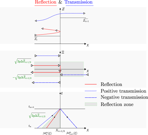
Figure 2: The potential bareer: transmission and reflection of particle

Top: the physical configuration
Middle: the characteristic solution in $(X,\Xi)$-plane
Bottom: the characteristic solution in $(X,t)$-plane

Due to the jump condition (33) and the sign of the kinetic speed, we distinguish three admissible cases as displayed on Fig. 2.

• The case $\xi_{l}>0$ corresponds to the positive transmission (this means that the particle comes from the left) and we deduce from Equalities (35) that the left microscopic flux $\mathcal{M}_{i+1/2}^{-}(\xi)$ is equal to $\displaystyle\mathcal{M}_{i}^{n}(\xi)$.

• The case $\xi_{l}<0$ and $\xi_{l}^{2}-2{g\Delta\widetilde{Z}_{i+1/2}}<0$ is the so-called reflection case. The condition $\xi_{l}^{2}-2{g\Delta\widetilde{Z}_{i+1/2}}<0$ says simply that the slope $\xi_{l}$ of the $X$ solution (35) cannot exceed $\sqrt{2g\Delta\widetilde{Z}_{i+1/2}}$ (as displayed on Fig. 2 (bottom)) and so the flux $\mathcal{M}_{i+1/2}^{-}(\xi)$ is given by $\mathcal{M}_{i}^{n}(-\xi)$. Physically, since the particle with the kinetic speed $\xi_{l}$, under the previous kinetic condition, has not enough energy to overpass the bareer, it is reflected with the kinetic speed $-\xi_{l}$.

• The last case is when $\xi_{l}<0$ and $\xi_{l}^{2}-2{g\Delta\widetilde{Z}_{i+1/2}}>0$. This case corresponds to the negative transmission: this means we take into account the particles coming from the right side with negative kinetic speed. Contrary to the reflection case, the constraint on the $X$ slope is limited by $\xi_{l}>-\sqrt{2g\Delta\widetilde{Z}_{i+1/2}}$ and we get as solution $\displaystyle\mathcal{M}_{i+1}^{n}\left(\displaystyle-\sqrt{\xi^{2}-2g\Delta\widetilde{Z}_{i+1/2}}\right)$. From a physical point of view, the observed particle at the left of the interface comes from the right side with a kinetic speed $\xi_{r}<0$ where $\displaystyle\xi_{r}=-\sqrt{\xi_{l}^{2}-2g\Delta\widetilde{Z}_{i+1/2}}$, taking into account the gain or loss of potential energy through the bareer (as displayed on Fig. 2 (bottom)).

Finally, adding the previous results we obtain:

$$\begin{array}[]{lll}\mathcal{M}_{i+1/2}^{-}(\xi)&=&\overbrace{\displaystyle\mathds{1}_{\xi>0}\mathcal{M}_{i}^{n}(\xi)}^{{positive\,\,\,transmission}}+\overbrace{\mathds{1}_{\xi<0,\xi^{2}-2g\Delta\widetilde{Z}_{i+1/2}<0}\mathcal{M}_{i}^{n}(-\xi)}^{reflection}\\ &+&\underbrace{\displaystyle\mathds{1}_{\xi<0,\xi^{2}-2g\Delta\widetilde{Z}_{i+1/2}>0}\mathcal{M}_{i+1}^{n}\left(\displaystyle-\sqrt{\xi^{2}-2g\Delta\widetilde{Z}_{i+1/2}}\right)}_{negative\,\,\,transmission}\\ &&\\ &&\\ \mathcal{M}_{i+1/2}^{+}(\xi)&=&\overbrace{\displaystyle\mathds{1}_{\xi<0}\mathcal{M}_{i+1}^{n}(\xi)}^{negative\,\,\,transmission}+\overbrace{\mathds{1}_{\xi>0,\xi^{2}+2g\Delta\widetilde{Z}_{i+1/2}<0}\mathcal{M}_{i+1}^{n}(-\xi)}^{reflection}\\ &+&\underbrace{\displaystyle\mathds{1}_{\xi>0,\xi^{2}+2g\Delta\widetilde{Z}_{i+1/2}>0}\mathcal{M}_{i}^{n}\left(\displaystyle\sqrt{\xi^{2}+2g\Delta\widetilde{Z}_{i+1/2}}\right)}_{positive\,\,\,transmission}\end{array}$$ (36)

The microscopic flux at the right of the interface is obtained following a same approach.

4.2 Numerical properties

We present some numerical properties of the macroscopic scheme (24)-(25), namely the stability and the preservation of the still water steady state. The stability of the kinetic scheme depends on a kinetic CFL condition

$$\frac{\Delta t^{n}}{\max_{i}h_{i}}\xi<1,\,\forall\xi$$

and so, on the support of the maxwellian function (e.g. we see that from the microscopic fluxes in Subsection 4.1). The support of the maxwellian function computed in Theorem 3.2 is not compact, then the stability condition cannot be satisfied. Therefore, in the sequel, we will consider the particular Gibbs equilibrium $\chi(w)=\displaystyle\frac{1}{2\sqrt{3}}\mathds{1}_{[-\sqrt{3},\sqrt{3}]}(w)$ introduced by the authors in [2] and used in [6] in the case of pressurised flows in uniform closed pipe.

Let us present the numerical properties of the scheme (26)-(36),

Theorem 4.1

2. Assuming the CFL condition

   $$\frac{\Delta t^{n}}{\max_{i\in\mathbb{Z}}h_{i}}\max_{i\in\mathbb{Z}}\left(|\overline{U}_{i}^{n}|+\sqrt{3}c\right)<1,$$

   the numerical scheme (26)-(36) keeps the wet equivalent area $A$ positive.

3. The still water steady state is preserved:

   $$U_{i}^{n}=0,\quad\frac{c^{2}}{g}\ln(\rho_{i}^{n})+\widetilde{Z}_{i}=cst$$

Proof of Theorem 4.1. (It is similar to the one obtained in [9]) Let us suppose $A_{i}^{n}>0$ for all $i\in\mathbb{Z}$ and $n\in\mathbb{N}$. Let $\xi_{\pm}=\max(0,\pm\xi)$ be the positive or negative part of any real and $\sigma=\displaystyle\frac{\Delta t^{n}}{\max_{i}h_{i}}$, Equation (26) reads:

$$\begin{array}[]{lll}f_{i}^{n+1}(\xi)&\geqslant&(1-\sigma|\xi|)\mathcal{M}_{i}^{n}(\xi)\\ &&+\sigma\xi_{+}\left(\mathds{1}_{\xi^{2}+2g\Delta\widetilde{Z}_{i+1/2}<0}\mathcal{M}_{i}^{n}(-\xi)\right.\\ &&\left.+\mathds{1}_{\xi^{2}+2g\Delta\widetilde{Z}_{i-1/2}>0}\mathcal{M}_{i-1}^{n}\left(\displaystyle\sqrt{\xi^{2}+2g\Delta\widetilde{Z}_{i+1/2}}\right)\right)\\ &&+\sigma\xi_{-}\left(\mathds{1}_{\xi^{2}-2g\Delta\widetilde{Z}_{i+1/2}<0}\mathcal{M}_{i}^{n}(-\xi)\right.\\ &&\left.+\mathds{1}_{\xi^{2}-2g\Delta\widetilde{Z}_{i-1/2}>0}\mathcal{M}_{i+1}^{n}\left(\displaystyle-\sqrt{\xi^{2}-2g\Delta\widetilde{Z}_{i+1/2}}\right)\right)\end{array}$$

Since the support of the $\chi$ function is compact, we get

$$f_{i}^{n+1}(\xi)>0\text{ if }|\xi-u_{j}^{n}|<\sqrt{3}c,\,\forall j\in\mathbb{Z}$$

which implies $|\xi|<|u_{j}^{n}|+\sqrt{3}c$. Using the CFL condition $\sigma|\xi|\leq 1$, we get the result. Morever, since $f_{i}^{n+1}$ is a sum of positive term, we obtain $f_{i}^{n+1}>0$, hence the wet equivalent area at time $t^{n+1}$ is positive, i.e.

$$A_{i}^{n+1}=\displaystyle\int_{\mathbb{R}}f_{i}^{n+1}(\xi)\,d\xi>0.$$

To prove the second point, we distinguish cases $\xi>0$ and $\xi<0$ to show the equality $\mathcal{M}_{i+1/2}=\mathcal{M}_{i-1/2}$. Using the jump condition (33), we easily obtain $f_{i}^{n+1}=\mathcal{M}_{i}^{n}$ which gives the result.

$\square$

Now let us also remark that the kinetic scheme (27)-(36) is wet equivalent area conservative . Indeed, let us denote the first component of the discrete fluxes $\left(F_{A}\right)^{\pm}_{i+1/2}$:

$$\left(F_{A}\right)^{\pm}_{i+1/2}{:=}\int_{\mathbb{R}}\xi\mathcal{M}^{\pm}_{i+1/2}(\xi)\,d\xi$$

An easy computation, using the change of variables $w^{2}={\xi}^{2}-2g\Delta\widetilde{Z}_{i+1/2}$ in the interface densities formulas defining the kinetic fluxes $\mathcal{M}_{i+1/2}^{\pm}$, allows us to show that:

$$\left(F_{A}\right)^{+}_{i+\frac{1}{2}}=\left(F_{A}\right)^{-}_{i+\frac{1}{2}}$$

5 Numerical Validation

The validation is performed in the case of a soft and sharp water hammer in an uniform pipe. Then we compare the results to the ones provided by an industrial code used at EDF-CIH (France) (see [12]), which solves the Allievi equation by the method of characteristics. The validation in non uniform pipes is performed in the case of an immediate flow shut down in a quasi-frictionless cone-shaped pipe. The results are then compared to the equivalent pipe method [1].

5.1 The uniform case

We present now numerical results of a water hammer test. The pipe of circular cross-section of $2\mbox{ m}^{2}$ and thickness $20$ cm is $2000$ m long. The altitude of the upstream end of the pipe is $250$ m and the slope is $5^{\circ}$. The Young modulus is $23\,10^{9}\mbox{ Pa}$ since the pipe is supposed to be built in concrete. The total upstream head is 300 m. The initial downstream discharge is $10\mbox{ m}^{3}/\mbox{s}$ and we cut the flow in $10$ seconds for the first test case and in $5$ seconds for the other.

We present a validation of the proposed scheme by comparing numerical results of the proposed model solved by the kinetic scheme with the ones obtained by solving Allievi equations by the method of characteristics with the so-called belier code: an industrial code used by the engineers of the Center in Hydraulics Engineering of Electricité De France (EDF) [12].

A simulation of the water hammer test was done for a CFL coefficient equal to $0.8$ and a spatial discretisation of 1000 mesh points. In the figures Fig. 3 and Fig. 4, we present a comparison between the results obtained by our kinetic scheme and the ones obtained by the “belier” code: the behaviour of the discharge at the middle of the pipe. One can observe that the results for the proposed model are in very good agreement with the solution of Allievi equations. A little smoothing effect and absorption may be probably due to the first order discretisation type. A second order scheme may be implemented naturally and will produce a better approximation.

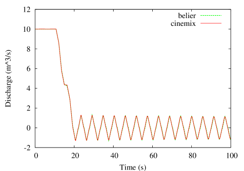
Figure 3: Comparison between the kinetic scheme and the industrial code belier

First case: discharge at the middle of the pipe

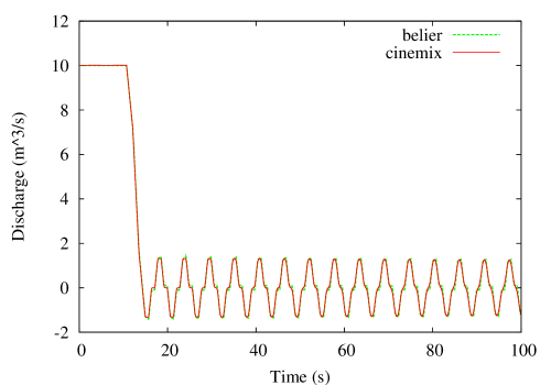
Figure 4: Comparison between the kinetic scheme and the industrial code belier

Second case: discharge at the middle of the pipe

5.2 The case of non uniform circular pipe

We present a test of the proposed kinetic scheme in the case of a contracting or expanding circular pipes of length $L=1000\,m$. The downstream radius is kept constant, equal to $R_{2}=1\,m$ and the upstream radius varies from $R_{1}=1\,m$ to $4\,m$ by steps of $0.25\,m$. The others paramaters are $N=300$ mesh points, $K_{S}=9000$ (this means that the wall of the pipe is very smooth), CFL$=0.8$. The upstream discharge before the shut-down ($1.5$ seconds) is fixed to $10\,m^{3}.s^{-1}$ while the upstream condition is a constant total head. We assume also that the pipe is rigid. Then for each value of the radius $R_{1}$, we compute the water hammer pressure rise at the position $x=96\,m$ of the pipe and we compare it to the one obtained by the equivalent pipe method (see [1]). The results are presented in Fig. 5 and show a very good agreement.

We point out that the behaviour of the solutions corresponding to the equivalent pipe method and our method are different: this is due to the dynamic treatment of the term $\displaystyle c^{2}\frac{d\ln S}{dX}$ related to the variable section which is not present in the equivalent pipe method: see Fig. 6, Fig. 7, Fig. 8 :

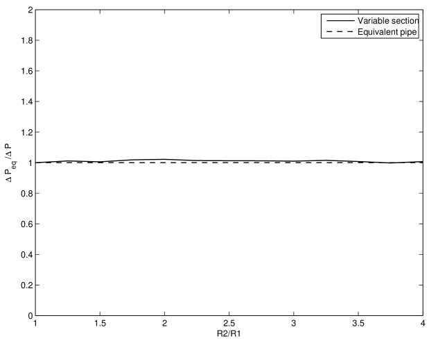
Figure 5: Comparison in the prediction of pressure rises in cone-shaped pipes between the present method and the equivalent pipe method

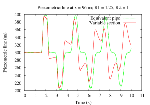
Figure 6: Discharge (left) and piezometric line (right) for $R_{1}=1.25\,m$

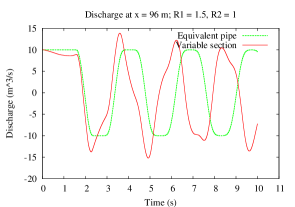
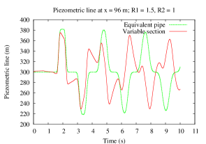
Figure 7: Discharge (left) and piezometric line (right) for $R_{1}=1.5\,m$

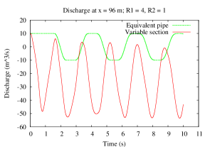
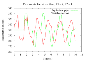
Figure 8: Discharge (left) and piezometric line (right) for $R_{1}=4\,m$

References

- [1] A. Adamkowski. Analysis of transient flow in pipes with expanding or contracting sections. ASME J. of Fluid Engineering, 125:716–722, 2003.
- [2] E. Audusse, M.O. Bristeau, and P. Perthame. Kinetic schemes for Saint-Venant equations with source terms on unstrucured grids. Technical Report RR-3989, INRIA, 2000.
- [3] F. Bouchut, E.D. Fernández-Nieto, A. Mangeney, and P.-Y. Lagrée. On new erosion models of savage-hutter type for avalanches. Acta Mech., 199:181–208, 2008.
- [4] C. Bourdarias, M. Ersoy, and S. Gerbi. A mathematical model for unsteady mixed flows in closed water pipes. http://hal.archives-ouvertes.fr/hal-00342745/fr/, 2008. (Submitted).
- [5] C. Bourdarias and S. Gerbi. A finite volume scheme for a model coupling free surface and pressurised flows in pipes. J. Comp. Appl. Math., 209(1):109–131, 2007.
- [6] C. Bourdarias, S. Gerbi, and M. Gisclon. A kinetic formulation for a model coupling free surface and pressurised flows in closed pipes. J. Comp. Appl. Math., 218(2):522–531, 2008.
- [7] H. Capart, X. Sillen, and Y. Zech. Numerical and experimental water transients in sewer pipes. Journal of Hydraulic Research, 35(5):659–672, 1997.
- [8] B. Perthame. Kinetic formulation of conservation laws. Oxford lecture series in mathematics and its applications. Oxford edition, 2002.
- [9] B. Perthame and C. Simeoni. A kinetic scheme for the Saint-Venant system with a source term. Calcolo, 38(4):201–231, 2001.
- [10] B. Perthame and E. Tadmor. A kinetic equations with kinetic entropy functions for scalar conservation laws. Comm. Math. Phys., 136(3):501–517, 1991.
- [11] V.L. Streeter, E.B. Wylie, and K.W. Bedford. Fluid Mechanics. McGraw-Hill, 1998.
- [12] V. Winckler. Logiciel belier4.0. Notes de principes. Technical report, EDF-CIH, Le Bourget du Lac, France, 1993.
- [13] E.B. Wylie and V.L. Streeter. Fluid Transients. McGraw-Hill, New York, 1978.