A model for unsteady mixed flows in non uniform closed water pipes and a well-balanced finite volume scheme

Christian Bourdarias, Mehmet Ersoy and Stéphane Gerbi
Laboratoire de Mathématiques, Université de Savoie
73376 Le Bourget du Lac, France
email: Christian.Bourdarias@univ-savoie.fr,email: Mehmet.Ersoy@univ-savoie.fr,email: Stephane.Gerbi@univ-savoie.fr
Abstract

We present the derivation of a new unidirectional model for unsteady mixed flows in non uniform closed water pipes. We introduce a local reference frame to take into account the local perturbation caused by the changes of section and slope. Then an asymptotic analysis is performed to obtain a model for free surface flows and another one for pressurized flows. By coupling these models through the transition points by the use of a common set of variables and a suitable pressure law, we obtain a simple formulation called PFS-model close to the shallow water equations with source terms. It takes into account the changes of section and the slope variation in a continuous way through transition points. Transition point between the two types of flows is treated as a free boundary associated to a discontinuity of the gradient of pressure. The numerical simulation is performed by making use of a Roe-like finite volume scheme that we adapted to take into account geometrical source terms in the convection matrix. Finally some numerical tests are presented.

Keywords : Shallow water, mixed flows, free surface flows, pressurized flows, curvilinear transformation, asymptotic analysis, VFRoe scheme, well-balanced finite volume scheme, hyperbolic system with source terms.

1 Introduction

The presented work takes place in a more general framework: the modelling of unsteady mixed flows in any kind of closed pipe taking into account the cavitation problem and air entrapment. We are interested in flows occurring in closed pipes with non uniform sections, where some parts of the flow can be free surface (it means that only a part of the pipe is filled) and other parts are pressurized (it means that the pipe is full). The transition phenomenon between the two types of flows occurs in many situations such as storm sewers, waste or supply pipes in hydroelectric installations. It can be induced by sudden changes in the boundary conditions as failure pumping. During this process, the pressure can reach severe values and may cause damages. The simulation of such a phenomenon is thus a major challenge and a great amount of works was devoted to it these last years (see [13],[14],[25],[29], for instance).

The classical shallow water equations are commonly used to describe free surface flows in open channels. They are also used in the study of mixed flows using the Preissman slot artefact (see for example [13, 29]). However, this technic does not take into account the depressurisation phenomenon which occurs during a water hammer except in recent works [21, 20, 22]. On the other hand the Allievi equations, commonly used to describe pressurized flows, are written in a non-conservative form which is not well adapted to a natural coupling with the shallow water equations.

A model for the unsteady mixed water flows in closed pipes and a finite volume discretisation have been previously studied by two of the authors [7] and a kinetic formulation has been proposed in [9]. We propose here the PFS-model which tends to extend naturally the work in [7] in the case of a closed pipe with non uniform section. For the sake of simplicity, we do not deal with the deformation of the domain induced by the change of pressure. We will consider only an infinitely rigid pipe.

The paper is organized as follows. Section 2 is devoted to the derivation of the free surface model from the 333D incompressible Euler equations which are written in a suitable local reference frame (following [3, 4]) in order to take into account the local effects produced by the changes of section and the slope variation. The construction of the free surface model is done by a formal asymptotic analysis. Seeking for an approximation at first order gives the model called FS-model. In Section 3, we adapt the derivation of the FS-model to derive the pressurized model, called P-model, from the 333D compressible Euler equations. Writing the source terms of these two models, P and FS-model, into a unified form and using the same couple of conservative unknowns as in [8], we propose in Section 4 a model for mixed flows, that we call PFS-model . We state some mathematical properties of this model. Section 5 is devoted to the extension of the VFRoe scheme described in [12, 16, 7] that was used for the case of uniform pipes. In Section 6, we show how to construct a convection matrix in order to get an exactly well-balanced scheme. Several numerical tests are presented in Section 7.

Notations concerning geometrical variables

  • (0,i,j,k)0ijk(0,{\textbf{i}},{\textbf{j}},{\textbf{k}}): cartesian reference frame

  • ω(x,0,b(x))𝜔𝑥0𝑏𝑥\omega(x,0,b(x)): parametrization in the reference frame (0,i,j,k)0ijk(0,{\textbf{i}},{\textbf{j}},{\textbf{k}}) of the plane curve 𝒞𝒞\mathcal{C} which corresponds to the main flow axis

  • (T,N,B)TNB(\textbf{T},\textbf{N},\textbf{B}): Serret-Frenet reference frame attached to 𝒞𝒞\mathcal{C} with T the tangent vector, N the normal vector and B the binormal vector

  • X,Y,Z𝑋𝑌𝑍X,Y,Z: local variable in the Serret Frenet reference frame with X𝑋X the curvilinear abscissa, Y𝑌Y the width of pipe, Z𝑍Z the B-coordinate of any particle.

  • σ(X,Z)=β(X,Z)α(X,Z)𝜎𝑋𝑍𝛽𝑋𝑍𝛼𝑋𝑍\sigma(X,Z)=\beta(X,Z)-\alpha(X,Z): width of the pipe at altitude Z𝑍Z with β(X,Z)𝛽𝑋𝑍\beta(X,Z) (resp. α(X,Z)𝛼𝑋𝑍\alpha(X,Z)) is the Y-coordinate of right (resp. left) boundary point at altitude Z𝑍Z

  • θ(X)𝜃𝑋\theta(X): angle (i,T)iT({\textbf{i}},\textbf{T})

  • S(X)𝑆𝑋S(X): cross-section area

  • R(X)𝑅𝑋R(X): radius of the cross-section S(X)𝑆𝑋S(X)

  • nwbsubscriptnwb{\textbf{n}}_{\textbf{wb}}: outward normal vector to the wet part of the pipe

  • n: outward normal vector at the boundary point m𝑚m in the ΩΩ\Omega-plane defined below

Notations concerning the free surface (FS) part

  • A𝐴A: wet area

  • Q𝑄Q: discharge

  • Ω(t,X)Ω𝑡𝑋\Omega(t,X): free surface cross section

  • H(t,X)𝐻𝑡𝑋H(t,X): physical water height

  • h(t,X)𝑡𝑋h(t,X): Z𝑍Z-coordinate of the water level, σ(X,h(t,X))=T(A)𝜎𝑋𝑡𝑋𝑇𝐴\sigma(X,h(t,X))=T(A) : width of the free surface

  • nfssubscriptnfs{\textbf{n}}_{\textbf{fs}}: outward B-normal vector to the free surface

  • ρ0subscript𝜌0\rho_{0}: density of the water at atmospheric pressure p0subscript𝑝0p_{0}

Notations concerning the pressurized part

  • Ω(X)Ω𝑋\Omega(X): pressurized cross section

  • ρ(t,X)𝜌𝑡𝑋\rho(t,X): density of the water

  • β𝛽\beta: water compressibility coefficient

  • c=1βρ0𝑐1𝛽subscript𝜌0c=\frac{1}{\sqrt{\beta\,\rho_{0}}}: sonic speed

  • A=ρρ0S𝐴𝜌subscript𝜌0𝑆A=\frac{\rho}{\rho_{0}}S: FS equivalent wet area

  • Q𝑄Q: FS equivalent discharge

Notations concerning the PFS model

  • S: the physical wet area: S=AS𝐴\mathcal{\textbf{S}}=A if the state is free surface, S𝑆S otherwise

  • \mathcal{H}: the Z𝑍Z coordinate of the water level: =h\mathcal{H}=h if the state is free surface, R𝑅R otherwise

Other notations

  • Bold characters are used for vectors except for S

2 Formal derivation of the FS-model for free surface flows

The classical shallow water equations are used to describe physical situations like rivers, coastal domains, oceans and sedimentation problems. These equations are obtained from the incompressible Euler system (see e.g. [2, 23]) or from the incompressible Navier-Stokes system (see for instance [10, 11, 17, 24]) by several techniques (e.g. by direct integration or asymptotic analysis). We adapt here the derivation in [3, 4] to get a new unidirectional shallow water model. We start from the 333D incompressible Euler equations where we neglect the acceleration following the y𝑦y-axis supposing the existence of a privileged main flow axis. We write then the Euler equations in the local Serret-Frenet reference frame in order to take into account the local effects produced by the changes of section and the slope variation. Then we derive a shallow water model by a formal asymptotic analysis (done in Subsection 2.3).

2.1 Incompressible Euler equations and framework

Let us consider the cartesian reference frame (O,i,j,k)𝑂ijk(O,{\textbf{i}},{\textbf{j}},{\textbf{k}}). In the corresponding coordinate system (x,y,z)𝑥𝑦𝑧(x,y,z), the 333D incompressible Euler system writes:

{div(ρ0U)=0t(ρ0U)+ρ0U(ρ0U)+P=Fcasesdivsubscript𝜌0U0subscript𝑡subscript𝜌0Usubscript𝜌0Usubscript𝜌0U𝑃F\left\{\begin{array}[]{rcl}{\rm div}(\rho_{0}\,{\textbf{U}})&=&0\\ \partial_{t}(\rho_{0}\,{\textbf{U}})+\rho_{0}\,{\textbf{U}}\cdot\nabla(\rho_{0}\,{\textbf{U}})+\nabla P&=&\textbf{F}\end{array}\right. (1)

where U(t,x,y,z)U𝑡𝑥𝑦𝑧{\textbf{U}}(t,x,y,z) denotes the velocity with components (u,v,w)𝑢𝑣𝑤(u,v,w), P=p(t,x,y,z)I3𝑃𝑝𝑡𝑥𝑦𝑧subscript𝐼3P=p(t,x,y,z)I_{3} is the isotropic pressure tensor, ρ0subscript𝜌0\rho_{0} the density of the fluid at atmospheric pressure p0subscript𝑝0p_{0} and F is the exterior strength of gravity.

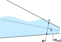
We close classically System (1) using a kinematic law for the evolution of the free surface: any free surface particle is advected by the fluid velocity U and on the wet boundary, we assume the no-leak condition U.nwb=0formulae-sequenceUsubscriptnwb0{\textbf{U}}.{\textbf{n}}_{\textbf{wb}}=0 where nwbsubscriptnwb{\textbf{n}}_{\textbf{wb}} is the outward unit normal vector to the wet part of the pipe (see Fig. 2). We set the pressure P𝑃P to 00 at the free surface.

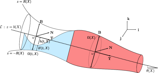
We define the domain ΩF(t)subscriptΩ𝐹𝑡\Omega_{F}(t) of the flow at time t𝑡t as the union of sections Ω(t,x)Ω𝑡𝑥\Omega(t,x) (assumed to be simply connected compact sets) orthogonal to some plane curve 𝒞𝒞\mathcal{C} lying in (O,i,k)𝑂ik(O,{\textbf{i}},{\textbf{k}}) to follow the privileged main flow axis. We choose the parametrization (x,0,b(x))𝑥0𝑏𝑥(x,0,b(x)) in the cartesian reference frame (O,i,j,k)𝑂ijk(O,{\textbf{i}},{\textbf{j}},{\textbf{k}}) where k follows the vertical direction; b(x)𝑏𝑥b(x) is then the elevation of the point ω(x,0,b(x))𝜔𝑥0𝑏𝑥\omega(x,0,b(x)) over the plane (O,i,j)𝑂ij(O,{\textbf{i}},{\textbf{j}}) (see Fig. 1).

We define a local reference frame as follows: we introduce the curvilinear variable defined by:

X=x0x1+(b(ξ))2𝑑ξ𝑋superscriptsubscriptsubscript𝑥0𝑥1superscriptsuperscript𝑏𝜉2differential-d𝜉\displaystyle X=\int_{x_{0}}^{x}\sqrt{1+(b^{\prime}(\xi))^{2}}d\xi

where x0subscript𝑥0x_{0} is an arbitrary abscissa. We set Y=y𝑌𝑦Y=y and we denote by Z𝑍Z the B-coordinate of any fluid particle M𝑀M in the Serret-Frenet reference frame (T,N,B)TNB(\textbf{T},\textbf{N},\textbf{B}) at point ω(x,0,b(x))𝜔𝑥0𝑏𝑥\omega(x,0,b(x)) with T the tangent vector N, the normal and B the binormal vector (see Fig. 1 and Fig. 3 for the notations). B is normal to 𝒞𝒞\mathcal{C} in the vertical plane (O,i,k)𝑂ik(O,{\textbf{i}},{\textbf{k}}).

Then, at each point ω𝜔\omega, Ω(t,X)Ω𝑡𝑋\Omega(t,X) is defined by the set:

{(y,Z)2;Z[R(X),R(X)+H(t,X)],y[α(X,Z),β(X,Z)]}formulae-sequence𝑦𝑍superscript2formulae-sequence𝑍𝑅𝑋𝑅𝑋𝐻𝑡𝑋𝑦𝛼𝑋𝑍𝛽𝑋𝑍\left\{(y,Z)\in\mathbb{R}^{2};Z\in[-R(X),-R(X)+H(t,X)],\,y\in[\alpha(X,Z),\beta(X,Z)]\right\}

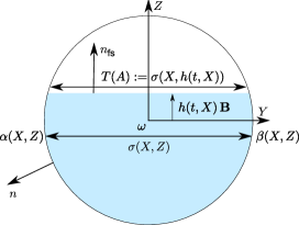
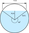
where R(X)𝑅𝑋R(X) denotes the radius, H(t,X)𝐻𝑡𝑋H(t,X) the physical water height at section Ω(t,X)Ω𝑡𝑋\Omega(t,X). We denote α(X,Z)𝛼𝑋𝑍\alpha(X,Z) (respectively β(X,Z))\beta(X,Z)) Y-coordinate of the left (respectively right) boundary point of the domain at altitude Z𝑍Z, R(X)<Z<R(X)𝑅𝑋𝑍𝑅𝑋-R(X)<Z<R(X) (see Fig. 3). We denote also R(X)+H(t,X)𝑅𝑋𝐻𝑡𝑋-R(X)+H(t,X) by h(t,X)𝑡𝑋h(t,X) which is the Z𝑍Z-coordinate of the water level.

Refer to caption
Figure 1: Geometric characteristics of the domain

Mixed flow: free surface and pressurized
Refer to caption
Figure 2: Outward unit normal nwbnsubscriptnwbn{\textbf{n}}_{\textbf{wb}}\neq{\textbf{n}} (except for uniform pipes)
Refer to caption
Figure 3: Cross-section Ω(t,X)Ω𝑡𝑋\Omega(t,X) of the domain at point ω𝜔\omega in the free surface case

In the sequel, we will use a curvilinear map which will be an admissible transformation under the geometrical hypothesis on the domain:

(H)𝐻(H)

Let (x)𝑥\mathcal{R}(x) be the algebraic curvature radius of the plane curve x(x,0,b(x))maps-to𝑥𝑥0𝑏𝑥x\mapsto(x,0,b(x)). We assume that:

xΩF,|(x)|>R(x).formulae-sequencefor-all𝑥subscriptΩ𝐹𝑥𝑅𝑥\forall x\in\Omega_{F},\,\,|\mathcal{R}(x)|>R(x).

2.2 Incompressible Euler model in the curvilinear coordinates

Following the work in [3, 4], we write System (1) in the Serret-Frenet reference frame (T,N,B)TNB(\textbf{T},\textbf{N},\textbf{B}) at point ω(x,0,b(x))𝜔𝑥0𝑏𝑥\omega(x,0,b(x)) by the transformation 𝒯:(x,y,z)(X,Y,Z):𝒯𝑥𝑦𝑧𝑋𝑌𝑍\mathcal{T}:(x,y,z)\rightarrow(X,Y,Z) using the divergence chain rule lemma that we recall here:

Lemma 2.1

Let (X,Y,Z)𝒯(X,Y,Z)=(x,y,z)maps-to𝑋𝑌𝑍𝒯𝑋𝑌𝑍𝑥𝑦𝑧(X,Y,Z)\mapsto\mathcal{T}(X,Y,Z)=(x,y,z) be a C1superscript𝐶1C^{1} diffeomorphism and
𝒜1=(X,Y,Z)𝒯superscript𝒜1subscript𝑋𝑌𝑍𝒯\mathcal{A}^{-1}=\nabla_{(X,Y,Z)}\mathcal{T} the jacobian matrix of the transformation with determinant J𝐽J.

Then, for any vector field ΦΦ\Phi, one has:

Jdiv(x,y,z)Φ=div(X,Y,Z)(J𝒜Φ),𝐽subscriptdiv𝑥𝑦𝑧Φsubscriptdiv𝑋𝑌𝑍𝐽𝒜ΦJ{\rm div}_{(x,y,z)}\Phi={\rm div}_{(X,Y,Z)}(J\mathcal{A}\Phi)\,,

and, for any scalar function f𝑓f, one has:

(x,y,z)f=𝒜t(X,Y,Z)f,subscript𝑥𝑦𝑧𝑓superscript𝒜𝑡subscript𝑋𝑌𝑍𝑓\nabla_{(x,y,z)}f=\mathcal{A}^{t}\nabla_{(X,Y,Z)}f,

where 𝒜tsuperscript𝒜𝑡\mathcal{A}^{t} stands for the transpose of the matrix 𝒜𝒜\mathcal{A}.

Let (U,V,W)tsuperscript𝑈𝑉𝑊𝑡(U,V,W)^{t} be the components of the velocity vector in the (X,Y,Z)𝑋𝑌𝑍(X,Y,Z) coordinates defined as (U,V,W)t=Θ(u,v,w)tsuperscript𝑈𝑉𝑊𝑡Θsuperscript𝑢𝑣𝑤𝑡(U,V,W)^{t}=\Uptheta(u,v,w)^{t} where ΘΘ\Uptheta is the matrix

Θ=(cosθ0sinθ010sinθ0cosθ),Θ𝜃0𝜃010𝜃0𝜃\Uptheta=\left(\begin{array}[]{ccc}\cos\theta&0&\sin\theta\\ 0&1&0\\ -\sin\theta&0&\cos\theta\\ \end{array}\right)\,,

where we denote by θ(x)𝜃𝑥\theta(x) the angle (i,T)iT({\textbf{i}},\textbf{T}) in the (i,k)ik({\textbf{i}},{\textbf{k}}) plane.

Using Lemma 2.1, the incompressible Euler system in the variables (X,Y,Z)𝑋𝑌𝑍(X,Y,Z) reads:

{X(ρ0U)+Y(Jρ0V)+Z(Jρ0W)=0t(Jρ0U)+X(ρ0U2)+Y(Jρ0UV)+Z(Jρ0UW)+Xp=G1t(Jρ0V)+X(ρ0UV)+Y(Jρ0V2)+Z(Jρ0VW)+Y(Jp)=0t(Jρ0W)+X(ρ0UW)+Y(Jρ0VW)+Z(Jρ0W2)+JZ(p)=G2casessubscript𝑋subscript𝜌0𝑈subscript𝑌𝐽subscript𝜌0𝑉subscript𝑍𝐽subscript𝜌0𝑊0subscript𝑡𝐽subscript𝜌0𝑈subscript𝑋subscript𝜌0superscript𝑈2subscript𝑌𝐽subscript𝜌0𝑈𝑉subscript𝑍𝐽subscript𝜌0𝑈𝑊subscript𝑋𝑝subscript𝐺1subscript𝑡𝐽subscript𝜌0𝑉subscript𝑋subscript𝜌0𝑈𝑉subscript𝑌𝐽subscript𝜌0superscript𝑉2subscript𝑍𝐽subscript𝜌0𝑉𝑊subscript𝑌𝐽𝑝0subscript𝑡𝐽subscript𝜌0𝑊subscript𝑋subscript𝜌0𝑈𝑊subscript𝑌𝐽subscript𝜌0𝑉𝑊subscript𝑍𝐽subscript𝜌0superscript𝑊2𝐽subscript𝑍𝑝subscript𝐺2\left\{\begin{array}[]{lll}\partial_{X}(\rho_{0}\,U)+\partial_{Y}(J\rho_{0}\,V)+\partial_{Z}(J\rho_{0}\,W)&=&0\\ \partial_{t}(J\rho_{0}\,U)+\partial_{X}(\rho_{0}\,U^{2})+\partial_{Y}(J\rho_{0}\,UV)+\partial_{Z}(J\rho_{0}\,UW)+\partial_{X}p&=&G_{1}\\ \partial_{t}(J\rho_{0}\,V)+\partial_{X}(\rho_{0}\,UV)+\partial_{Y}(J\rho_{0}\,V^{2})+\partial_{Z}(J\rho_{0}\,VW)+\partial_{Y}(Jp)&=&0\\ \partial_{t}(J\rho_{0}\,W)+\partial_{X}(\rho_{0}\,UW)+\partial_{Y}(J\rho_{0}\,VW)+\partial_{Z}(J\rho_{0}\,W^{2})+J\partial_{Z}(p)&=&G_{2}\end{array}\right. (2)

where J(X,Y,Z)=1Zθ(X)𝐽𝑋𝑌𝑍1𝑍superscript𝜃𝑋J(X,Y,Z)=1-Z\displaystyle\theta^{\prime}(X) is the determinant of the transformation and

G1=ρ0UWθ(X)Jgρ0sinθ,G2=ρ0U2θ(X)Jgρ0cosθ.formulae-sequencesubscript𝐺1subscript𝜌0𝑈𝑊superscript𝜃𝑋𝐽𝑔subscript𝜌0𝜃subscript𝐺2subscript𝜌0superscript𝑈2superscript𝜃𝑋𝐽𝑔subscript𝜌0𝜃G_{1}=\rho_{0}\,UW\theta^{\prime}(X)-Jg\rho_{0}\,\sin\theta,\,\,G_{2}=-\rho_{0}\,U^{2}\theta^{\prime}(X)-Jg\rho_{0}\,\cos\theta.

The interested reader can find the details of the calculus in [3]. We have denoted by fsuperscript𝑓f^{\prime} the derivative with respect to the space variable X𝑋X of any function f(X)𝑓𝑋f(X).

On the wet boundary, the no-leak condition reads:

(U,V,W)t.nwb=0.formulae-sequencesuperscript𝑈𝑉𝑊𝑡subscriptnwb0\displaystyle({U},{V},{W})^{t}.{\textbf{n}}_{\textbf{wb}}=0\,. (3)
Remark 2.1

Notice that κ(X)=θ(X)𝜅𝑋superscript𝜃𝑋\kappa(X)=\displaystyle\theta^{\prime}(X) is the algebraic curvature of the axis at point ω(X,0,b(X))𝜔𝑋0𝑏𝑋\omega(X,0,b(X)) and the function J(X,Y,Z)=1Zκ(X)𝐽𝑋𝑌𝑍1𝑍𝜅𝑋J(X,Y,Z)=1-Z\kappa(X) depends only on the variables X,Z𝑋𝑍X,Z. Moreover, under the hypothesis (H)𝐻(H), we have J>0𝐽0J>0 in ΩFsubscriptΩ𝐹\Omega_{F}. Consequently, 𝒯𝒯\mathcal{T} defines a diffeomorphism and thus the performed transformation is admissible.

2.3 Formal derivation of the FS-model for free surface flows

In this section, we perform a formal asymptotic analysis on System (2). According to the work in [3, 17, 24], the shallow water equations can be obtained from the incompressible Navier-Stokes equations with particular boundary conditions. Here, we perform this analysis directly on the incompressible Euler system in order to get J=1+O(ϵ)𝐽1𝑂italic-ϵJ=1+O(\epsilon) for some small parameter ϵitalic-ϵ\epsilon.

Let us introduce the usual small parameter ϵ=H/Litalic-ϵ𝐻𝐿\epsilon=H/L where H𝐻H (the height) and L𝐿L (the length) are two characteristics dimensions along the B and T axis respectively. Moreover, we assume that the characteristic dimension along the j axis is the same as for the k axis. We introduce the other characteristics dimensions T,P,U¯,V¯,W¯𝑇𝑃¯𝑈¯𝑉¯𝑊T,P,\overline{U},\overline{V},\overline{W} for time, pressure and velocity respectively and the dimensionless quantities as follows:

U~=U/U¯,V~=ϵV/U¯,W~=ϵW/U¯,formulae-sequence~𝑈𝑈¯𝑈formulae-sequence~𝑉italic-ϵ𝑉¯𝑈~𝑊italic-ϵ𝑊¯𝑈\widetilde{U}=U/\overline{U},\,\widetilde{V}=\epsilon V/\overline{U},\,\widetilde{W}=\epsilon{W}/{\overline{U}},\,
X~=X/L,Y~=Y/H,Z~=Z/H,p~=p/P,θ~=θ,ρ~=ρ0.formulae-sequence~𝑋𝑋𝐿formulae-sequence~𝑌𝑌𝐻formulae-sequence~𝑍𝑍𝐻formulae-sequence~𝑝𝑝𝑃formulae-sequence~𝜃𝜃~𝜌subscript𝜌0\widetilde{X}={X}/{L},\,\widetilde{Y}={Y}/{H},\,\widetilde{Z}={Z}/{H},\,\widetilde{p}={p}/{P},\widetilde{\theta}={\theta},\widetilde{\rho}={\rho_{0}}.

In the sequel, we set P=U¯2𝑃superscript¯𝑈2P={\overline{U}}^{2} and L=TU¯𝐿𝑇¯𝑈L=T\overline{U} (i.e. we only consider laminar flows).

Under these hypotheses, we have J~(X~,Y~,Z~)=1ϵZ~θ~(X~)~𝐽~𝑋~𝑌~𝑍1italic-ϵ~𝑍superscript~𝜃~𝑋\widetilde{J}(\widetilde{X},\widetilde{Y},\widetilde{Z})=1-\epsilon\widetilde{Z}\displaystyle\widetilde{\theta}^{\prime}(\widetilde{X}). Thus, the rescaled System (2) reads:

{X~U~+Y~(J~V~)+Z~(J~W~)=0t~(J~U~)+X~(U~2)+Y~(J~U~V~)+Z~(J~U~W~)+X~p~=G1ϵ2(t~(J~V~)+X~(U~V~)+Y~(J~V~2)+Z~(J~V~W~))+Y~(J~p~)=0ϵ2(t~(J~W~)+X~(U~W~)+Y~(J~V~W~)+Z~(J~W~2))+J~Z~(p~)=G2casessubscript~𝑋~𝑈subscript~𝑌~𝐽~𝑉subscript~𝑍~𝐽~𝑊0subscript~𝑡~𝐽~𝑈subscript~𝑋superscript~𝑈2subscript~𝑌~𝐽~𝑈~𝑉subscript~𝑍~𝐽~𝑈~𝑊subscript~𝑋~𝑝subscript𝐺1superscriptitalic-ϵ2subscript~𝑡~𝐽~𝑉subscript~𝑋~𝑈~𝑉subscript~𝑌~𝐽superscript~𝑉2subscript~𝑍~𝐽~𝑉~𝑊subscript~𝑌~𝐽~𝑝0superscriptitalic-ϵ2subscript~𝑡~𝐽~𝑊subscript~𝑋~𝑈~𝑊subscript~𝑌~𝐽~𝑉~𝑊subscript~𝑍~𝐽superscript~𝑊2missing-subexpressionmissing-subexpression~𝐽subscript~𝑍~𝑝subscript𝐺2missing-subexpressionmissing-subexpression\left\{\begin{array}[]{rcl}\partial_{\widetilde{X}}\widetilde{U}+\partial_{\widetilde{Y}}(\widetilde{J}\widetilde{V})+\partial_{\widetilde{Z}}(\widetilde{J}\widetilde{W})&=&0\\ \partial_{\widetilde{t}}(\widetilde{J}\widetilde{U})+\partial_{\widetilde{X}}({\widetilde{U}}^{2})+\partial_{\widetilde{Y}}(\widetilde{J}\widetilde{U}\widetilde{V})+\partial_{\widetilde{Z}}(\widetilde{J}\widetilde{U}\widetilde{W})+\partial_{\widetilde{X}}\widetilde{p}&=&G_{1}\\ \epsilon^{2}\left(\partial_{\widetilde{t}}(\widetilde{J}\widetilde{V})+\partial_{\widetilde{X}}(\widetilde{U}\widetilde{V})+\partial_{\widetilde{Y}}(\widetilde{J}{\widetilde{V}}^{2})+\partial_{\widetilde{Z}}(\widetilde{J}\widetilde{V}\widetilde{W})\right)+\partial_{\widetilde{Y}}(\widetilde{J}\widetilde{p})&=&0\\ \epsilon^{2}\left(\partial_{\widetilde{t}}(\widetilde{J}\widetilde{W})+\partial_{\widetilde{X}}(\widetilde{U}\widetilde{W})+\partial_{\widetilde{Y}}(\widetilde{J}\widetilde{V}\widetilde{W})+\partial_{\widetilde{Z}}(\widetilde{J}{\widetilde{W}}^{2})\right)\\ +\widetilde{J}\partial_{\widetilde{Z}}(\widetilde{p})=G_{2}\end{array}\right. (4)

where

G1=ϵU~W~κ~(X~)sinθ~Fr,L2Z~Fr,H2(cosθ~),subscript𝐺1italic-ϵ~𝑈~𝑊~𝜅~𝑋~𝜃superscriptsubscript𝐹𝑟𝐿2~𝑍superscriptsubscript𝐹𝑟𝐻2superscript~𝜃G_{1}=\epsilon\widetilde{U}\widetilde{W}\widetilde{\kappa}(\widetilde{X})-\displaystyle\frac{\sin\widetilde{\theta}}{{F_{r,L}}^{2}}-\frac{\widetilde{Z}\displaystyle}{{F_{r,H}}^{2}}(\cos\widetilde{\theta})^{\prime},
G2=ϵU~2ρ~(X~)cosθ~Fr,H2+ϵκ(X)Z~J~cosθ~Fr,H2,subscript𝐺2italic-ϵsuperscript~𝑈2~𝜌~𝑋~𝜃superscriptsubscript𝐹𝑟𝐻2italic-ϵ𝜅𝑋~𝑍~𝐽~𝜃superscriptsubscript𝐹𝑟𝐻2G_{2}=-\epsilon{\widetilde{U}}^{2}\widetilde{\rho}(\widetilde{X})-\displaystyle\frac{\cos\widetilde{\theta}}{{F_{r,H}}^{2}}+\displaystyle\epsilon\kappa(X)\frac{\widetilde{Z}\widetilde{J}\cos\widetilde{\theta}}{{F_{r,H}}^{2}},

Fr,M=U¯gMsubscript𝐹𝑟𝑀¯𝑈𝑔𝑀F_{r,M}=\displaystyle\frac{\overline{U}}{\sqrt{gM}} is the Froude number along the T axis and the B or N axis where M𝑀M is any generic variable equal to L𝐿L or H𝐻H.

Formally, when ϵitalic-ϵ\epsilon vanishes, System (4) reduces to:

X~U~+Y~(V~)+Z~(W~)subscript~𝑋~𝑈subscript~𝑌~𝑉subscript~𝑍~𝑊\displaystyle\partial_{\widetilde{X}}\widetilde{U}+\partial_{\widetilde{Y}}(\widetilde{V})+\partial_{\widetilde{Z}}(\widetilde{W}) =\displaystyle= 00\displaystyle 0 (5)
t~(U~)+X~(U~2)+Y~(U~V~)+Z~(U~W~)+X~p~subscript~𝑡~𝑈subscript~𝑋superscript~𝑈2subscript~𝑌~𝑈~𝑉subscript~𝑍~𝑈~𝑊subscript~𝑋~𝑝\displaystyle\partial_{\widetilde{t}}(\widetilde{U})+\partial_{\widetilde{X}}(\widetilde{U}^{2})+\partial_{\widetilde{Y}}(\widetilde{U}\widetilde{V})+\partial_{\widetilde{Z}}(\widetilde{U}\widetilde{W})+\partial_{\widetilde{X}}\widetilde{p} =\displaystyle= sinθ~Fr,L2~𝜃superscriptsubscript𝐹𝑟𝐿2\displaystyle-\displaystyle\frac{\sin\widetilde{\theta}}{{F_{r,L}}^{2}} (6)
Z~Fr,H2(cosθ~)~𝑍superscriptsubscript𝐹𝑟𝐻2superscript~𝜃\displaystyle-\displaystyle\frac{\widetilde{Z}\displaystyle}{{F_{r,H}}^{2}}(\cos\widetilde{\theta})^{\prime}
Z~(p~)subscript~𝑍~𝑝\displaystyle\partial_{\widetilde{Z}}(\widetilde{p}) =\displaystyle= cosθ~Fr,H2~𝜃superscriptsubscript𝐹𝑟𝐻2\displaystyle-\displaystyle\frac{\cos\widetilde{\theta}}{{F_{r,H}}^{2}} (7)

Let us introduce the conservative variables A(t,X)𝐴𝑡𝑋A(t,X) and Q(t,X)𝑄𝑡𝑋Q(t,X) representing respectively the wet area and the discharge defined as:

A(t,X)=Ω(t,X)𝑑Y𝑑Z,Q(t,X)=A(t,X)U¯formulae-sequence𝐴𝑡𝑋subscriptΩ𝑡𝑋differential-d𝑌differential-d𝑍𝑄𝑡𝑋𝐴𝑡𝑋¯𝑈A(t,X)=\int_{\Omega(t,X)}dYdZ,\quad Q(t,X)=A(t,X)\overline{U}

where U¯¯𝑈\overline{U} is the mean value of the velocity :

U¯(t,X)=1A(t,X)Ω(t,X)U(t,X)𝑑Y𝑑Z.¯𝑈𝑡𝑋1𝐴𝑡𝑋subscriptΩ𝑡𝑋𝑈𝑡𝑋differential-d𝑌differential-d𝑍\overline{U}(t,X)=\frac{1}{A(t,X)}\int_{\Omega(t,X)}U(t,X)\,\,dYdZ\,.

We integrate the preceding system (5-6-7) along the cross-section with the approximation U2¯U¯U¯¯superscript𝑈2¯𝑈¯𝑈\overline{U^{2}}\approx\overline{U}\,\overline{U} and UV¯U¯V¯¯𝑈𝑉¯𝑈¯𝑉\overline{U\,V}\approx\overline{U}\,\overline{V}. Then, returning to the physical variables, the free surface model, that we call FS-model, reads:

{tA+XQ=0tQ+X(Q2A+gI1(X,A)cosθ)=gI2(X,A)cosθgAsinθgAZ¯(X,A)(cosθ)casessubscript𝑡𝐴subscript𝑋𝑄0subscript𝑡𝑄subscript𝑋superscript𝑄2𝐴𝑔subscript𝐼1𝑋𝐴𝜃𝑔subscript𝐼2𝑋𝐴𝜃𝑔𝐴𝜃missing-subexpressionmissing-subexpression𝑔𝐴¯𝑍𝑋𝐴superscript𝜃\left\{\begin{array}[]{lll}\partial_{t}A+\partial_{X}Q&=&0\\ \displaystyle\partial_{t}Q+\displaystyle\partial_{X}\left(\frac{Q^{2}}{A}+\displaystyle gI_{1}(X,A)\cos\theta\right)&=&\displaystyle gI_{2}(X,A)\cos\theta-gA\sin\theta\\ &&-gA\overline{Z}(X,A)\displaystyle{(\cos\theta)^{\prime}}\end{array}\right. (8)

where I1(X,A)subscript𝐼1𝑋𝐴I_{1}(X,A) and I2(X,A)subscript𝐼2𝑋𝐴I_{2}(X,A) are respectively the classical term of hydrostatic pressure and the pressure source term defined by:

I1(X,A)=Rh(hZ)σ𝑑Z and I2(X,A)=Rh(hZ)XσdZsubscript𝐼1𝑋𝐴superscriptsubscript𝑅𝑍𝜎differential-d𝑍 and subscript𝐼2𝑋𝐴superscriptsubscript𝑅𝑍subscript𝑋𝜎𝑑𝑍I_{1}(X,A)=\int_{-R}^{h}(h-Z)\sigma\,dZ\textrm{ and }I_{2}(X,A)=\int_{-R}^{h}(h-Z)\partial_{X}\sigma\,dZ

which are obtained from the integration of the pressure term X~p~subscript~𝑋~𝑝\partial_{\widetilde{X}}\widetilde{p} in Equation (5) with p~=ρ(h(t,X)Z)cosθ~𝑝𝜌𝑡𝑋𝑍𝜃\widetilde{p}=\rho(h(t,X)-Z)\cos\theta (obtained from equation (7)).

In these formulas σ(X,Z)𝜎𝑋𝑍\sigma(X,Z) is the width of the cross-section at position X𝑋X and at height Z𝑍Z. The additional term Z¯(X,A)¯𝑍𝑋𝐴\overline{Z}(X,A) is defined by (h(A)I1(X,A)/A)𝐴subscript𝐼1𝑋𝐴𝐴(h(A)-I_{1}(X,A)/A). It is the Z𝑍Z-coordinate of the center of mass:

Z¯=Ω(t,X)Z𝑑Y𝑑Z=R(X)h(t,X)α(X,Z)β(X,Z)Z𝑑Y𝑑Z=R(X)h(t,X)Zσ(X,Z)𝑑Z.¯𝑍subscriptΩ𝑡𝑋𝑍differential-d𝑌differential-d𝑍missing-subexpressionsuperscriptsubscript𝑅𝑋𝑡𝑋superscriptsubscript𝛼𝑋𝑍𝛽𝑋𝑍𝑍differential-d𝑌differential-d𝑍missing-subexpressionsuperscriptsubscript𝑅𝑋𝑡𝑋𝑍𝜎𝑋𝑍differential-d𝑍\begin{array}[]{lll}\overline{Z}&=&\displaystyle\int_{\Omega(t,X)}Z\,dY\,dZ\\ &=&\displaystyle\int_{-R(X)}^{h(t,X)}\int_{\alpha(X,Z)}^{\beta(X,Z)}Z\,dY\,dZ\\ &=&\displaystyle\int_{-R(X)}^{h(t,X)}Z\,\sigma(X,Z)\,dZ\end{array}\,.

In System (8), we may add a friction term ρ0gSfTsubscript𝜌0𝑔subscript𝑆𝑓T-\rho_{0}gS_{f}\,\textbf{T} to take into account the dissipation of energy. We have chosen this term Sfsubscript𝑆𝑓S_{f} as the one given by the Manning-Strickler law (see e.g. [29]):

Sf(A,U)=K(A)U|U|.subscript𝑆𝑓𝐴𝑈𝐾𝐴𝑈𝑈S_{f}(A,U)=K(A)U|U|\,.

The term K(A)𝐾𝐴K(A) is defined by: K(A)=1Ks2Rh(A)4/3𝐾𝐴1superscriptsubscript𝐾𝑠2subscript𝑅superscript𝐴43\displaystyle K(A)=\frac{1}{K_{s}^{2}R_{h}(A)^{4/3}}, Ks>0subscript𝐾𝑠0K_{s}>0 is the Strickler coefficient of roughness depending on the material, Rh(A)=A/Pmsubscript𝑅𝐴𝐴subscript𝑃𝑚R_{h}(A)=A/P_{m} is the hydraulic radius and Pmsubscript𝑃𝑚P_{m} is the perimeter of the wet surface area (length of the part of the channel’s section in contact with the water).

3 Formal derivation of the P-model for pressurized flows

In this section, we present a new set of unidirectional shallow water like equations to describe pressurized flows in closed non uniform water pipes. This model is constructed to be coupled in natural way with the FS-model (8). Starting from the 333D compressible Euler equations in cartesian coordinates,

tρ+div(ρU)=0,subscript𝑡𝜌div𝜌U0\partial_{t}\rho+{\rm div}{(\rho{\textbf{U}})}=0, (9)
t(ρU)+div(ρUU)+p=F,subscript𝑡𝜌Udivtensor-product𝜌UU𝑝F\partial_{t}(\rho{\textbf{U}})+{\rm div}{(\rho{\textbf{U}}\otimes{\textbf{U}})}+\nabla p=\textbf{F}, (10)

where U(t,x,y,z)U𝑡𝑥𝑦𝑧{\textbf{U}}(t,x,y,z) and ρ(t,x,y,z))\rho(t,x,y,z)) denotes the velocity with components (u,v,w)𝑢𝑣𝑤(u,v,w) and the density respectively. p(t,x,y,z)𝑝𝑡𝑥𝑦𝑧p(t,x,y,z) is the scalar pressure and F the exterior strength of gravity.

We define the pressurized domain of the flow as the continuous extension of ΩFsubscriptΩ𝐹\Omega_{F} (see Subsection 2.1) defined by some plane curve 𝒞𝒞\mathcal{C} with parametrization (x,0,b(x))𝑥0𝑏𝑥(x,0,b(x)) in the cartesian reference frame (O,i,j,k)𝑂ijk(O,{\textbf{i}},{\textbf{j}},{\textbf{k}}); we recall that b(x)𝑏𝑥b(x) is then the elevation of the point ω𝜔\omega over the plane (O,i,j)𝑂ij(O,{\textbf{i}},{\textbf{j}}) (see Fig. 1). The curve may be, for instance, the axis spanned by the center of mass of each orthogonal section Ω(x)Ω𝑥\Omega(x) to the main mean flow axis, particularly in the case of a piecewise cone-shaped pipe. Notice that we consider only the case of infinitely rigid pipes, thus the sections Ω=Ω(x)ΩΩ𝑥\Omega=\Omega(x) are only x𝑥x-dependent.

We then write Equations (9-10) in the (X,Y,Z)𝑋𝑌𝑍(X,Y,Z) coordinates introduced in Subsection 2.1. As we want a unidirectional model, we suppose that the mean flow follows the X𝑋X-axis. To this end, we neglect the second and third equation for the conservation of the momentum.
By a straightforward computation, the mass and the first momentum conservation equation in the (X,Y,Z)𝑋𝑌𝑍(X,Y,Z) coordinates reads:

{t(Jρ)+X(ρU)+Y(ρJV)+Z(ρJW)=0t(JρU)+X(ρU2)+Y(ρJUV2)+Z(ρJUW)+Xp=ρJgsinθ+ρUW(cosθ)casessubscript𝑡𝐽𝜌subscript𝑋𝜌𝑈subscript𝑌𝜌𝐽𝑉subscript𝑍𝜌𝐽𝑊0missing-subexpressionmissing-subexpressionmissing-subexpressionsubscript𝑡𝐽𝜌𝑈subscript𝑋𝜌superscript𝑈2subscript𝑌𝜌𝐽𝑈superscript𝑉2subscript𝑍𝜌𝐽𝑈𝑊subscript𝑋𝑝missing-subexpressionmissing-subexpressionabsent𝜌𝐽𝑔𝜃𝜌𝑈𝑊superscript𝜃missing-subexpressionmissing-subexpression\left\{\begin{array}[]{rcl}\partial_{t}(J\rho)+\partial_{X}(\rho U)+\partial_{Y}(\rho JV)+\partial_{Z}(\rho JW)&=&0\\ &&\\ \partial_{t}(J\rho U)+\partial_{X}(\rho U^{2})+\partial_{Y}(\rho JUV^{2})+\partial_{Z}(\rho JUW)+\partial_{X}p\\ =-\rho Jg\sin\theta+\rho UW\displaystyle(\cos\theta)^{\prime}\end{array}\right. (11)

Applying the same asymptotic analysis developed in Subsection 2.3, Equations (9-10) read:

{t(ρ)+X(ρU)+Y(ρV)+Z(ρW)=0t(ρU)+X(ρU2)+Y(ρUV)+Z(ρUW)+Xp=ρgsinθgZ(cosθ)casessubscript𝑡𝜌subscript𝑋𝜌𝑈subscript𝑌𝜌𝑉subscript𝑍𝜌𝑊0missing-subexpressionmissing-subexpressionmissing-subexpressionsubscript𝑡𝜌𝑈subscript𝑋𝜌superscript𝑈2subscript𝑌𝜌𝑈𝑉subscript𝑍𝜌𝑈𝑊subscript𝑋𝑝𝜌𝑔𝜃missing-subexpressionmissing-subexpression𝑔𝑍superscript𝜃\left\{\begin{array}[]{rcl}\partial_{t}(\rho)+\partial_{X}({\rho U})+\partial_{Y}(\rho V)+\partial_{Z}(\rho W)&=&0\\ &&\\ \partial_{t}(\rho U)+\partial_{X}({\rho U}^{2})+\partial_{Y}(\rho UV)+\partial_{Z}(\rho UW)+\partial_{X}p&=&-\rho\displaystyle{g\sin\theta}\\ &&-gZ\displaystyle(\cos\theta)^{\prime}\end{array}\right. (12)

We choose the linearized pressure law:

p=pa+ρρ0βρ0𝑝subscript𝑝𝑎𝜌subscript𝜌0𝛽subscript𝜌0p=p_{a}+\displaystyle{\frac{\rho-\rho_{0}}{\beta\rho_{0}}} (13)

(see e.g. [29, 30]) in which ρ0subscript𝜌0\rho_{0} represents the density of the fluid at atmospheric pressure p0subscript𝑝0p_{0}, pasubscript𝑝𝑎p_{a} is some function set to zero and β𝛽\beta the water compressibility coefficient (equal to 5.0 1010m2.N1formulae-sequencesuperscript5.01010superscript𝑚2superscript𝑁15.0\,10^{-10}\,m^{2}.N^{-1} in practice). The sonic speed is then given by c= 1/βρ0𝑐1𝛽subscript𝜌0c\leavevmode\nobreak\ =\leavevmode\nobreak\ 1/\sqrt{\beta\rho_{0}} and thus c1400m.s1formulae-sequence𝑐1400𝑚superscript𝑠1c\approx 1400\,m.s^{-1}.
For mΩ𝑚Ωm\in\partial\Omega, n=m|m|nmm\displaystyle{\textbf{n}}=\frac{{\textbf{m}}}{|{\textbf{m}}|} is the outward unit vector at the point m𝑚m in the ΩΩ\Omega-plane and m stands for the vector ωm𝜔𝑚{\omega m} (as displayed on Fig. 3).

Following the section-averaging method performed in Subsection 2.3, we integrate System (12) over the cross-section ΩΩ\Omega. Noting the averaged values over ΩΩ\Omega by the overlined letters (except Z¯¯𝑍\overline{Z}), and using the approximations ρU¯ρ¯U¯,ρU2¯ρ¯U¯2formulae-sequence¯𝜌𝑈¯𝜌¯𝑈¯𝜌superscript𝑈2¯𝜌superscript¯𝑈2\overline{\rho U}\approx\overline{\rho}\overline{U},\,\overline{\rho U^{2}}\approx\overline{\rho}\overline{U}^{2} the shallow water like equations read:

t(ρ¯S)+X(ρ¯SU¯)subscript𝑡¯𝜌𝑆subscript𝑋¯𝜌𝑆¯𝑈\displaystyle\partial_{t}(\overline{\rho}S)+\partial_{X}({\overline{\rho}S\overline{U}}) =\displaystyle= Ωρ(UXmV).ndsformulae-sequencesubscriptΩ𝜌𝑈subscript𝑋mVn𝑑𝑠\displaystyle\displaystyle\int_{\partial\Omega}\rho\left(U\partial_{X}{\textbf{m}}-\textbf{V}\right).{\textbf{n}}\,ds (14)
t(ρ¯SU¯)+X(ρ¯SU¯+c2ρ¯S)subscript𝑡¯𝜌𝑆¯𝑈subscript𝑋¯𝜌𝑆¯𝑈superscript𝑐2¯𝜌𝑆\displaystyle\partial_{t}(\overline{\rho}S\overline{U})+\partial_{X}(\displaystyle\overline{\rho}S\overline{U}+c^{2}\overline{\rho}S) =\displaystyle= gρ¯Ssinθ+c2ρ¯S𝑔¯𝜌𝑆𝜃superscript𝑐2¯𝜌superscript𝑆\displaystyle-\displaystyle{g\overline{\rho}S\sin\theta}+c^{2}\overline{\rho}S^{\prime}
\displaystyle- gρ¯SZ¯(cosθ)𝑔¯𝜌𝑆¯𝑍superscript𝜃\displaystyle g\overline{\rho}S\overline{Z}\displaystyle(\cos\theta)^{\prime}
+\displaystyle+ ΩρU(UXmV).ndsformulae-sequencesubscriptΩ𝜌𝑈𝑈subscript𝑋mVn𝑑𝑠\displaystyle\displaystyle\int_{\partial\Omega}\rho U\left(U\partial_{X}{\textbf{m}}-\textbf{V}\right).{\textbf{n}}\,ds

where V=(V,W)tVsuperscript𝑉𝑊𝑡\textbf{V}=(V,W)^{t} is the velocity in the (N,B)NB(\textbf{N},\textbf{B})-plane. We denote by S𝑆S the area of the cross-section of the pipe at position X𝑋X.

The integral terms appearing in (14) and (3) vanish, as the pipe is infinitely rigid, i.e. Ω=Ω(X)ΩΩ𝑋\Omega=\Omega(X) (see [8] for the dilatable case). It follows the non-penetration condition (see Fig. 4):

(UVW).nwb=0.formulae-sequence𝑈𝑉𝑊subscriptnwb0\left(\begin{array}[]{c}U\\ V\\ W\end{array}\right).{\textbf{n}}_{\textbf{wb}}=0\,.

Omitting the overlined letters (except Z¯¯𝑍\overline{Z}), we introduce the conservative variables

A=ρρ0S𝐴𝜌subscript𝜌0𝑆\displaystyle A=\displaystyle\frac{\rho}{\rho_{0}}S the FS equivalent wet area (16)
Q=AU𝑄𝐴𝑈\displaystyle Q=\displaystyle AU the FS equivalent discharge.the FS equivalent discharge\displaystyle\textrm{ the FS \emph{equivalent discharge}}\,. (17)

and dividing Equations (14)-(3) by ρ0subscript𝜌0\rho_{0} we get:

{t(A)+X(Q)=0t(Q)+X(Q2A+c2A)=gAsinθgAZ¯(X,S)(cosθ)+c2ASScasessubscript𝑡𝐴subscript𝑋𝑄0missing-subexpressionmissing-subexpressionmissing-subexpressionsubscript𝑡𝑄subscript𝑋superscript𝑄2𝐴superscript𝑐2𝐴𝑔𝐴𝜃𝑔𝐴¯𝑍𝑋𝑆superscript𝜃missing-subexpressionmissing-subexpressionsuperscript𝑐2𝐴superscript𝑆𝑆\left\{\begin{array}[]{rcl}\partial_{t}(A)+\partial_{X}(Q)&=&0\\ &&\\ \partial_{t}(Q)+\partial_{X}\left(\displaystyle\frac{Q^{2}}{A}+c^{2}A\right)&=&-\displaystyle{gA\sin\theta}-gA\overline{Z}(X,S)\displaystyle(\cos\theta)^{\prime}\\ &&+\displaystyle c^{2}A\frac{S^{\prime}}{S}\end{array}\right. (18)

As introduced previously for the FS-model in Section (2.3), we may introduce the friction term ρgSfT𝜌𝑔subscript𝑆𝑓T-\rho gS_{f}\,\textbf{T} given by the Manning-Strickler law (see e.g. [29]):

Sf(S,U)=K(S)U|U|subscript𝑆𝑓𝑆𝑈𝐾𝑆𝑈𝑈S_{f}(S,U)=K(S)U|U|

where K(S)𝐾𝑆K(S) is defined by: K(S)=1Ks2Rh(S)4/3𝐾𝑆1superscriptsubscript𝐾𝑠2subscript𝑅superscript𝑆43\displaystyle K(S)=\frac{1}{K_{s}^{2}R_{h}(S)^{4/3}}, Ks>0subscript𝐾𝑠0K_{s}>0 is the Strickler coefficient of roughness depending on the material and Rh(S)=S/Pmsubscript𝑅𝑆𝑆subscript𝑃𝑚R_{h}(S)=S/P_{m} is the hydraulic radius where Pmsubscript𝑃𝑚P_{m} is the perimeter of the wet surface area (length of the part of the channel’s section in contact with the water, equal to 2πR2𝜋𝑅2\,\pi\,R in the case of circular pipe).

This choice of variables is motivated by the fact that this system is formally close to the FS-model (8) where the terms gI1(X,A)cosθ𝑔subscript𝐼1𝑋𝐴𝜃gI_{1}(X,A)\cos\theta, gI2(X,A)cosθ𝑔subscript𝐼2𝑋𝐴𝜃gI_{2}(X,A)\cos\theta, Z¯(X,A)¯𝑍𝑋𝐴\overline{Z}(X,A) are respectively the counterparts of c2Asuperscript𝑐2𝐴c^{2}A, c2ASSsuperscript𝑐2𝐴superscript𝑆𝑆\displaystyle c^{2}A\frac{S^{\prime}}{S}, Z¯(X,S)¯𝑍𝑋𝑆\overline{Z}(X,S) in System (18). Let us remark that the term Z¯¯𝑍\overline{Z} is continuous through the change of state (pressurized to free surface or free surface to pressurized state) when the same curve plane is chosen (in practice, the main axis of the pipe). Then, we are motivated to connect “continuously” System (8) and (18) through transition points (through the change of state) by defining a continuous pressure law. It leads to a “natural” coupling between the pressurized and free surface model as we will see in Section 4.

4 The PFS-model

The formulations of the FS-model (8) and P-model (18) are very close to each other. The main difference comes from the pressure law. In order to build a coupling between the two models, we have to define a pressure that ensures its continuity through transition points in the same spirit of [7]. As pointed out in the previous section, we will use the common couple of unknowns (A,Q)𝐴𝑄(A,Q) and the same plane curve 𝒞𝒞\mathcal{C} (see Remark 4.1) to get a continuous model for mixed flows.

Remark 4.1

The plane curve with parametrization (x,0,b(x))𝑥0𝑏𝑥(x,0,b(x)) is chosen as the main pipe axis in the axisymmetric case. Actually this choice is the more convenient for pressurized flows while the bottom line is adapted to free surface flows. Thus we must assume small variations of the section (Ssuperscript𝑆\displaystyle S^{\prime} small) or equivalently small angle φ𝜑\varphi as displayed on Fig. 4.

Refer to caption
Figure 4: Some restriction concerning the geometric domain.

We introduce a state indicator E𝐸E (see Fig. 5) such that:

E={1 if the state is pressurized: (ρρ0)0 if the state is free surface: (ρ=ρ0).𝐸cases1 if the state is pressurized: 𝜌subscript𝜌00 if the state is free surface: 𝜌subscript𝜌0E=\left\{\begin{array}[]{ll}1&\textrm{ if the state is pressurized: }(\rho\neq\rho_{0})\\ 0&\textrm{ if the state is free surface: }(\rho=\rho_{0})\\ \end{array}\right.\,. (19)

Next, we define the physical wet area S by:

S=S(A,E)={S if E=1A if E=0SS𝐴𝐸cases𝑆 if 𝐸1𝐴 if 𝐸0\mathcal{\textbf{S}}=\mathcal{\textbf{S}}(A,E)=\left\{\begin{array}[]{lll}S&\textrm{ if }&E=1\\ A&\textrm{ if }&E=0\end{array}\right. (20)

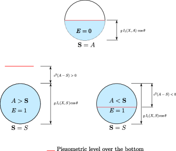
and a modified pressure law (see Fig. 5) which ensures its continuity through the change of state by:

p(X,A,E)=c2(AS)+gI1(X,S)cosθ.𝑝𝑋𝐴𝐸superscript𝑐2𝐴S𝑔subscript𝐼1𝑋S𝜃p(X,A,E)=c^{2}(A-\mathcal{\textbf{S}})+gI_{1}(X,\mathcal{\textbf{S}})\cos\theta. (21)
Remark 4.2
  • Indeed, when a change of state occurs we have:

    limA<SASp(X,A,E)=limA>SASp(X,A,E)=gI1(X,S)cos(θ)subscriptsuperscript𝐴𝑆𝐴𝑆𝑝𝑋𝐴𝐸subscriptsuperscript𝐴𝑆𝐴𝑆𝑝𝑋𝐴𝐸𝑔subscript𝐼1𝑋𝑆𝜃\lim_{\stackrel{{\scriptstyle A\to S}}{{A<S}}}p(X,A,E)=\lim_{\stackrel{{\scriptstyle A\to S}}{{A>S}}}p(X,A,E)=gI_{1}(X,S)\cos(\theta)

    which ensures the continuity of the pressure.

  • The flux gradient F𝐹F is discontinuous through the change of state since

    FA(A,Q,0)=gAI1(X,A)cosθc2=FA(A,Q,1).𝐹𝐴𝐴𝑄0𝑔𝐴subscript𝐼1𝑋𝐴𝜃superscript𝑐2𝐹𝐴𝐴𝑄1\frac{\partial F}{\partial A}(A,Q,0)=g\frac{\partial}{\partial A}I_{1}(X,A)\cos\theta\neq c^{2}=\frac{\partial F}{\partial A}(A,Q,1).

Finally, from the P-model (18), the FS-model (8), the definition of E𝐸E (19), the definition of S (20) and the pressure law (21), the PFS-model for unsteady mixed flows can be simply expressed into a single formulation as:

{t(A)+X(Q)=0t(Q)+X(Q2A+p(X,A,E))=gAb+Pr(X,A,E)G(X,A,E)K(X,A,E)Q|Q|Acasessubscript𝑡𝐴subscript𝑋𝑄0subscript𝑡𝑄subscript𝑋superscript𝑄2𝐴𝑝𝑋𝐴𝐸𝑔𝐴superscript𝑏𝑃𝑟𝑋𝐴𝐸missing-subexpressionmissing-subexpression𝐺𝑋𝐴𝐸missing-subexpressionmissing-subexpression𝐾𝑋𝐴𝐸𝑄𝑄𝐴\left\{\begin{array}[]{rcl}\partial_{t}(A)+\partial_{X}({Q})&=&0\\ \partial_{t}(Q)+\partial_{X}\left(\displaystyle\frac{Q^{2}}{A}+p(X,A,E)\right)&=&-\displaystyle gA\displaystyle b^{\prime}+Pr(X,A,E)\\ &&-G(X,A,E)\\ &&-K(X,A,E)\displaystyle\frac{Q|Q|}{A}\end{array}\right. (22)

where K𝐾K, Pr𝑃𝑟Pr, and G𝐺G denotes respectively the friction, the pressure source and the geometry source term defined as follows:

Pr(X,A,E)=c2(AS1)S+gI2(X,S)cosθ with I2(X,S)=R(X)(S)((S)Z)Xσ(X,Z)dZ,G(X,A,E)=gAZ¯(X,S)(cosθ),K(X,A,E)=1Ks2Rh(S)4/3𝑃𝑟𝑋𝐴𝐸superscript𝑐2𝐴S1superscript𝑆𝑔subscript𝐼2𝑋S𝜃missing-subexpressionmissing-subexpression with subscript𝐼2𝑋Ssuperscriptsubscript𝑅𝑋SS𝑍subscript𝑋𝜎𝑋𝑍𝑑𝑍𝐺𝑋𝐴𝐸𝑔𝐴¯𝑍𝑋Ssuperscript𝜃𝐾𝑋𝐴𝐸1superscriptsubscript𝐾𝑠2subscript𝑅superscriptS43\begin{array}[]{lll}Pr(X,A,E)&=&\displaystyle c^{2}\left(\frac{A}{\mathcal{\textbf{S}}}-1\right)\,S^{\prime}+gI_{2}(X,\mathcal{\textbf{S}})\cos\theta\\ &&\textrm{ with }I_{2}(X,\mathcal{\textbf{S}})=\displaystyle\int_{-R(X)}^{\mathcal{H}(\mathcal{\textbf{S}})}(\mathcal{H}(\mathcal{\textbf{S}})-Z)\,\partial_{X}\sigma(X,Z)\,dZ,\\ G(X,A,E)&=&\displaystyle gA\,\overline{Z}(X,\mathcal{\textbf{S}})\displaystyle(\cos\theta)^{\prime},\\ K(X,A,E)&=&\displaystyle\frac{1}{K_{s}^{2}R_{h}(\mathcal{\textbf{S}})^{4/3}}\end{array}

and bsuperscript𝑏b^{\prime} stands for sinθ(X)𝜃𝑋\sin\theta(X). \mathcal{H} represents the Z𝑍Z-coordinate of the water level:

=(S)={h(A) if E=0R(X) if E=1.Scases𝐴 if 𝐸0𝑅𝑋 if 𝐸1\mathcal{H}=\mathcal{H}(\mathcal{\textbf{S}})=\left\{\begin{array}[]{lll}h(A)&\textrm{ if }&E=0\\ R(X)&\textrm{ if }&E=1\end{array}\right.\,. (23)
Remark 4.3 (Both models are recovered)

Setting S(A,E)=AS𝐴𝐸𝐴\mathcal{\textbf{S}}(A,E)=A in System (22), we obtain obviously the free surface model (8). For all pressurized states, when S(A,E)=SS𝐴𝐸𝑆\mathcal{\textbf{S}}(A,E)=S, the pressure law (21) reads, for instance, in the case of circular pipe:

c2(AS)+gI1(X,S)cosθ=c2(AS)+gπR3cosθsuperscript𝑐2𝐴𝑆𝑔subscript𝐼1𝑋𝑆𝜃superscript𝑐2𝐴𝑆𝑔𝜋superscript𝑅3𝜃c^{2}(A-S)+gI_{1}(X,S)\cos\theta=c^{2}(A-S)+g\,\pi\,R^{3}\,\cos\theta

which is not exactly the pressure law of the P-model (18). Indeed, the derivation of the P-model is done with the linearized pressure law (13) (see Section 3) with pa=0subscript𝑝𝑎0p_{a}=0. Thus, the property of the continuity of models (18)-(8) through a change of state is obtained if and only if pasubscript𝑝𝑎p_{a} is chosen as gI1(X,S)cosθ𝑔subscript𝐼1𝑋𝑆𝜃gI_{1}(X,S)\cos\theta which is the hydrostatic pressure corresponding to a full section.
Refer to caption
Figure 5: Free surface state p(X,A,0)=gI1(X,A)cosθ𝑝𝑋𝐴0𝑔subscript𝐼1𝑋𝐴𝜃p(X,A,0)=g\,I_{1}(X,A)\cos\theta (top), pressurized state with overpressure p(x,A,1)>0𝑝𝑥𝐴10p(x,A,1)>0 (bottom left), pressurized state with depression p(x,A,1)<0𝑝𝑥𝐴10p(x,A,1)<0 (bottom right).

The PFS-model (22) satisfies the following properties:

Theorem 4.1
  1. 1.

    The right eigenvalues of System (22) are given by:

    λ=Uc(A,E),λ+=U+c(A,E)formulae-sequencesuperscript𝜆𝑈𝑐𝐴𝐸superscript𝜆𝑈𝑐𝐴𝐸\lambda^{-}=U-c(A,E),\,\lambda^{+}=U+c(A,E)

    with c(A,E)={gAT(A)cosθ if E=0c if E=1,𝑐𝐴𝐸cases𝑔𝐴𝑇𝐴𝜃 if 𝐸0𝑐 if 𝐸1c(A,E)=\left\{\begin{array}[]{lll}\displaystyle\sqrt{g\,\frac{A}{T(A)}\,\cos\theta}&\textrm{ if }&E=0\\ \displaystyle c&\textrm{ if }&E=1\end{array}\right.\,, where T(A)𝑇𝐴T(A) is the width of the free surface (see Fig. 3).

    Then, System (22) is strictly hyperbolic on the set:

    {A(t,X)>0}.𝐴𝑡𝑋0\left\{A(t,X)>0\right\}\,.
  2. 2.

    For smooth solutions, the mean velocity U=Q/A𝑈𝑄𝐴U=Q/A satisfies

    tU+X(U22+c2ln(A/S)+g(S)cosθ+gb)=gK(X,A,E)U|U|0.subscript𝑡𝑈subscript𝑋superscript𝑈22superscript𝑐2𝐴S𝑔S𝜃𝑔𝑏absent𝑔𝐾𝑋𝐴𝐸𝑈𝑈0\begin{array}[]{c}\partial_{t}U+\partial_{X}\left(\displaystyle\frac{U^{2}}{2}+c^{2}\ln(A/\mathcal{\textbf{S}})+g\mathcal{H}(\mathcal{\textbf{S}})\cos\theta+gb\right)\\ =-gK(X,A,E)U|U|\leqslant 0.\end{array} (24)

    The quantity U22+c2ln(A/S)+g(S)cosθ+gbsuperscript𝑈22superscript𝑐2𝐴S𝑔S𝜃𝑔𝑏\displaystyle\frac{U^{2}}{2}+c^{2}\ln(A/\mathcal{\textbf{S}})+g\mathcal{H}(\mathcal{\textbf{S}})\cos\theta+gb is called the total head.

  3. 3.

    The still water steady state reads:

    u=0 and c2ln(A/S)+g(S)cosθ+gb=0.𝑢0 and superscript𝑐2𝐴S𝑔S𝜃𝑔𝑏0u=0\;\mbox{ and }\;c^{2}\ln(A/\mathcal{\textbf{S}})+g\mathcal{H}(\mathcal{\textbf{S}})\cos\theta+gb=0. (25)
  4. 4.

    It admits a mathematical entropy

    (A,Q,E)=Q22A+c2Aln(A/S)+c2S+gAZ¯(X,S)cosθ+gAb𝐴𝑄𝐸superscript𝑄22𝐴superscript𝑐2𝐴𝐴Ssuperscript𝑐2𝑆𝑔𝐴¯𝑍𝑋S𝜃𝑔𝐴𝑏\mathcal{E}(A,Q,E)=\displaystyle\frac{Q^{2}}{2A}+c^{2}A\ln(A/\mathcal{\textbf{S}})+c^{2}S+gA\overline{Z}(X,\mathcal{\textbf{S}})\cos\theta+gAb (26)

    which satisfies the entropy relation for smooth solutions

    t+X((+p(X,A,E))U)=gAK(X,A,E)U2|U|0.subscript𝑡subscript𝑋𝑝𝑋𝐴𝐸𝑈𝑔𝐴𝐾𝑋𝐴𝐸superscript𝑈2𝑈0\partial_{t}\mathcal{E}+\partial_{X}\Big{(}\left(\mathcal{E}+p(X,A,E)\right)U\Big{)}=-gAK(X,A,E)U^{2}|U|\leqslant 0\,. (27)

Notice that the total head and \mathcal{E} are defined continuously through the transition points.

Remark 4.4

The term AZ¯(X,A)(cosθ)𝐴¯𝑍𝑋𝐴superscript𝜃A\overline{Z}(X,A)(\cos\theta)^{\prime} is also called “corrective term” since it allows to write the Equations (24) and (27) with (26).

Proof of Theorem 4.1: the results (24) and (27) are obtained in a classical way. Indeed, Equation (24) is obtained by subtracting the result of the multiplication of the mass equation by U𝑈U to the momentum equation. Then multiplying the mass equation by (U22+c2ln(A/S)+g(S)cosθ+gb)superscript𝑈22superscript𝑐2𝐴S𝑔S𝜃𝑔𝑏\left(\displaystyle\frac{U^{2}}{2}+c^{2}\ln(A/\mathcal{\textbf{S}})+g\mathcal{H}(\mathcal{\textbf{S}})\cos\theta+gb\right) and adding the result of the multiplication of Equation (24) by Q𝑄Q, we get:

t(Q22A+c2Aln(A/S)+c2S+gAZ¯(X,S)cosθ+gAb)+X((Q22A+c2Aln(A/S)+c2S+gAZ¯(X,S)cosθ+gAb+p(X,A,E))U)+c2(AS1)tS=gAK(X,A,E)U2|U|0.subscript𝑡superscript𝑄22𝐴superscript𝑐2𝐴𝐴Ssuperscript𝑐2𝑆𝑔𝐴¯𝑍𝑋S𝜃𝑔𝐴𝑏subscript𝑋superscript𝑄22𝐴superscript𝑐2𝐴𝐴Ssuperscript𝑐2𝑆𝑔𝐴¯𝑍𝑋S𝜃𝑔𝐴𝑏𝑝𝑋𝐴𝐸𝑈superscript𝑐2𝐴S1subscript𝑡S𝑔𝐴𝐾𝑋𝐴𝐸superscript𝑈2𝑈0\begin{array}[]{l}\partial_{t}\left(\displaystyle\frac{Q^{2}}{2A}+c^{2}A\ln(A/\mathcal{\textbf{S}})+c^{2}S+gA\overline{Z}(X,\mathcal{\textbf{S}})\cos\theta+gAb\right)\\ +\partial_{X}\left(\left(\displaystyle\frac{Q^{2}}{2A}+c^{2}A\ln(A/\mathcal{\textbf{S}})+c^{2}S+gA\overline{Z}(X,\mathcal{\textbf{S}})\cos\theta+gAb+p(X,A,E)\right)U\right)\\ +c^{2}\left(\displaystyle\frac{A}{\mathcal{\textbf{S}}}-1\right)\partial_{t}\mathcal{\textbf{S}}=-gAK(X,A,E)U^{2}|U|\leqslant 0\,.\end{array}

We see that the term c2(AS1)tSsuperscript𝑐2𝐴S1subscript𝑡Sc^{2}\left(\displaystyle\frac{A}{\mathcal{\textbf{S}}}-1\right)\partial_{t}\mathcal{\textbf{S}} is identically 00 since we have S=AS𝐴\mathcal{\textbf{S}}=A when the flow is free surface whereas S=S(X)S𝑆𝑋\mathcal{\textbf{S}}=S(X) when the flow is pressurized. Moreover, from the last inequality, when S=AS𝐴\mathcal{\textbf{S}}=A, we have the classical entropy inequality (see [7, 8]) with \mathcal{E}:

(A,Q,E)=Q22A+gAZ¯(X,A)cosθ+gAb𝐴𝑄𝐸superscript𝑄22𝐴𝑔𝐴¯𝑍𝑋𝐴𝜃𝑔𝐴𝑏\mathcal{E}(A,Q,E)=\displaystyle\frac{Q^{2}}{2A}+gA\overline{Z}(X,A)\cos\theta+gAb

while in the pressurized case, it is:

(A,Q,E)=Q22A+c2Aln(A/S)+c2S+gAb.𝐴𝑄𝐸superscript𝑄22𝐴superscript𝑐2𝐴𝐴𝑆superscript𝑐2𝑆𝑔𝐴𝑏\mathcal{E}(A,Q,E)=\displaystyle\frac{Q^{2}}{2A}+c^{2}A\ln(A/S)+c^{2}S+gAb.

Finally, the entropy for the PFS-model reads:

(A,Q,E)=Q22A+c2Aln(A/S)+c2S+gAZ¯(X,S)cosθ+gAb.𝐴𝑄𝐸superscript𝑄22𝐴superscript𝑐2𝐴𝐴Ssuperscript𝑐2𝑆𝑔𝐴¯𝑍𝑋S𝜃𝑔𝐴𝑏\mathcal{E}(A,Q,E)=\displaystyle\frac{Q^{2}}{2A}+c^{2}A\ln(A/\mathcal{\textbf{S}})+c^{2}S+gA\overline{Z}(X,\mathcal{\textbf{S}})\cos\theta+gAb.

Let us remark that the term c2Ssuperscript𝑐2𝑆c^{2}S makes \mathcal{E} continuous through transition points and it permits also to write the entropy flux under the classical form (+p)U𝑝𝑈(\mathcal{E}+p)U.

\blacksquare

5 Finite volume discretisation

In this section, we adapt the VFRoe scheme described in [12, 16, 7]. The new terms appearing in the PFS-model related to the curvature and the section variation are upwinded in the same spirit of [7]. The numerical scheme is adapted to discontinuities of the flux gradient occurring in the treatment of the transitions between free surface and pressurized states.

5.1 Discretisation of the space domain

The spatial domain is a pipe of length L𝐿L. The main axis of the pipe is divided in cells mi=[Xi1/2,Xi+12], 1iNformulae-sequencesubscript𝑚𝑖subscript𝑋𝑖12subscript𝑋𝑖121𝑖𝑁\displaystyle m_{i}=[X_{i-1/2},X_{i+\frac{1}{2}}],\ 1\leq i\leq N. ΔtnΔsuperscript𝑡𝑛\Delta t^{n} denotes the timestep and we set tn+1=tn+Δtnsubscript𝑡𝑛1subscript𝑡𝑛Δsuperscript𝑡𝑛t_{n+1}=t_{n}+\Delta t^{n}.
The discrete unknowns are Uin=(AinQin)superscriptsubscript𝑈𝑖𝑛superscriptsubscript𝐴𝑖𝑛superscriptsubscript𝑄𝑖𝑛U_{i}^{n}=\left(\begin{array}[]{c}A_{i}^{n}\\ Q_{i}^{n}\end{array}\right). For the sake of simplicity, the boundary conditions are not treated (the interested reader can find this treatment in details in [7]).

5.2 Explicit first order VFRoe scheme

We propose to extend the finite volume discretisation [7] to the PFS-model using the upwinding of the new source terms: the curvature and section variation of the pipe. In what follows, we do not write the E𝐸E dependency.

First, following Leroux et al. [18, 26] we use piecewise constant functions to approximate b𝑏b (b(X)=sinθ(X))superscript𝑏𝑋𝜃𝑋(b^{\prime}(X)=\sin\theta(X)) as well as the term cosθ𝜃\cos\theta and the cross section area S𝑆S. Adding the equations tZ=0subscript𝑡𝑍0\partial_{t}Z=0, tcosθ=0subscript𝑡𝜃0\partial_{t}\cos\theta=0 and tS=0subscript𝑡𝑆0\partial_{t}S=0, the PFS-model can be written under a non-conservative form with the variable W=(b,cosθ,S,A,Q)tWsuperscript𝑏𝜃𝑆𝐴𝑄𝑡\textbf{W}=(b,\cos\theta,S,A,Q)^{t}:

tW+XF(X,W)+B(X,W)XW=TS(W)subscript𝑡Wsubscript𝑋F𝑋W𝐵𝑋Wsubscript𝑋W𝑇𝑆W\partial_{t}\textbf{W}+\partial_{X}\textbf{F}(X,\textbf{W})+B(X,\textbf{W})\partial_{X}\textbf{W}=TS(\textbf{W}) (28)

where

F(X,W)=(000QQ2A+p(X,A)), TS(W)=(0000gK(X,S)Q|Q|A)formulae-sequenceF𝑋W000𝑄superscript𝑄2𝐴𝑝𝑋𝐴 𝑇𝑆W0000𝑔𝐾𝑋S𝑄𝑄𝐴\textbf{F}(X,\textbf{W})=\left(\begin{array}[]{c}0\\ 0\\ 0\\ Q\\ \displaystyle\frac{Q^{2}}{A}+p(X,A)\end{array}\right),\textrm{ }TS(\textbf{W})=\left(\begin{array}[]{c}0\\ 0\\ 0\\ 0\\ \displaystyle-g\,K(X,\mathcal{\textbf{S}})\,\frac{Q|Q|}{A}\end{array}\right)

and

B(X,W)=(00000000000000000000gAgAZ¯c2(A/S1)(X,W)00)𝐵𝑋W00000000000000000000𝑔𝐴𝑔𝐴¯𝑍superscript𝑐2𝐴S1𝑋W00B(X,\textbf{W})=\left(\begin{array}[]{ccccc}0&0&0&0&0\\ 0&0&0&0&0\\ 0&0&0&0&0\\ 0&0&0&0&0\\ gA&gA\overline{Z}&-c^{2}(A/\mathcal{\textbf{S}}-1)-\mathcal{I}(X,\textbf{W})&0&0\end{array}\right)\quad

where we have written the pressure source term due to the geometry gI2(X,S)cos(θ)𝑔subscript𝐼2𝑋S𝜃gI_{2}(X,\mathcal{\textbf{S}})\cos(\theta) as (X,W)S𝑋Wsuperscript𝑆\mathcal{I}(X,\textbf{W})S^{\prime}. For instance, for a circular cross-section pipe we have:

(X,W)=12π((S)π2+(S)arcsin((S)R(X))+σ(X,(S))2).𝑋W12𝜋S𝜋2SS𝑅𝑋𝜎𝑋S2\mathcal{I}(X,\textbf{W})=\frac{1}{2\,\pi}\left(\displaystyle\frac{\mathcal{H}(\mathcal{\textbf{S}})\pi}{2}+\mathcal{H}(\mathcal{\textbf{S}})\arcsin\left(\frac{\mathcal{H}(\mathcal{\textbf{S}})}{R(X)}\right)+\frac{\sigma(X,\mathcal{H}(\mathcal{\textbf{S}}))}{2}\right)\,.

Let Winsuperscriptsubscript𝑊𝑖𝑛W_{i}^{n} be an approximation of the mean value of W on the mesh misubscript𝑚𝑖m_{i} at time tnsubscript𝑡𝑛t_{n}. Since the values of b,cosθ,S𝑏𝜃𝑆b,\cos\theta,S are known, integrating the above equations over ]Xi1/2,Xi+12[×[tn,tn+1[]X_{i-1/2},X_{i+\frac{1}{2}}[\times[t_{n},t_{n+1}[, we can write a Finite Volume scheme as follows:

Win+1=Winαi(F(Wi+1/2(0,Win,Wi+1n))F(Wi1/2(0+,Wi1n,Win)))+TS(Win)superscriptsubscriptW𝑖𝑛1superscriptsubscriptW𝑖𝑛subscript𝛼𝑖FsubscriptsuperscriptW𝑖12superscript0superscriptsubscriptW𝑖𝑛superscriptsubscriptW𝑖1𝑛FsubscriptsuperscriptW𝑖12superscript0superscriptsubscriptW𝑖1𝑛superscriptsubscriptW𝑖𝑛missing-subexpressionmissing-subexpression𝑇𝑆subscriptsuperscriptW𝑛𝑖\begin{array}[]{lll}\textbf{W}_{i}^{n+1}&=&\textbf{W}_{i}^{n}\displaystyle-\displaystyle\alpha_{i}\left(\textbf{F}(\textbf{W}^{*}_{i+1/2}(0^{-},\textbf{W}_{i}^{n},\textbf{W}_{i+1}^{n}))-\textbf{F}(\textbf{W}^{*}_{i-1/2}(0^{+},\textbf{W}_{i-1}^{n},\textbf{W}_{i}^{n}))\right)\\ &&+\displaystyle TS(\textbf{W}^{n}_{i})\end{array} (29)

with αi=Δtnhi.subscript𝛼𝑖Δsuperscript𝑡𝑛subscript𝑖\alpha_{i}=\displaystyle\frac{\Delta t^{n}}{h_{i}}.

Wi+1/2(ξ=x/t,Wi,Wi+1)subscriptsuperscriptW𝑖12𝜉𝑥𝑡subscriptW𝑖subscriptW𝑖1\textbf{W}^{*}_{i+1/2}(\xi=x/t,\textbf{W}_{i},\textbf{W}_{i+1}) is the exact or an approximate solution to the Riemann problem at interface Xi+1/2subscript𝑋𝑖12X_{i+1/2} associated to the left and right states WisubscriptW𝑖\textbf{W}_{i} and Wi+1subscriptW𝑖1\textbf{W}_{i+1}. Let us also remark that the term B(X,W)𝐵𝑋WB(X,\textbf{W}) does not appear explicitly in this formulation since bsuperscript𝑏b^{\prime}, (cosθ)superscript𝜃(\cos\theta)^{\prime} and Ssuperscript𝑆S^{\prime} are null on ]Xi1/2,Xi+12[]X_{i-1/2},X_{i+\frac{1}{2}}[ but contributes to the computation of the numerical flux.

The computation of the interface quantities Wi±1/2(0±,Wi,Wi+1)subscriptsuperscriptWplus-or-minus𝑖12superscript0plus-or-minussubscriptW𝑖subscriptW𝑖1\textbf{W}^{*}_{i\pm 1/2}(0^{\pm},\textbf{W}_{i},\textbf{W}_{i+1}) will depend on two types of interfaces located at the point Xi+12subscript𝑋𝑖12X_{i+\frac{1}{2}} : the first one is a non transition point, when the flow on both sides of the interface is of the same type. The second one is a transition point, when the flow changes of type through the interface. We recall the approach used in [7] and adapt it here to the new terms. According to the type of interface, we have to solve two different linearised Riemann problems.

5.2.1 The Case of a non transition point

Expanding the term XF(X,W)subscript𝑋F𝑋W\partial_{X}\textbf{F}(X,\textbf{W}) in the non-conservative equations (28), the quasilinear formulation of the PFS-model (22) reads:

tW+D(W)XW=TS(W)subscript𝑡W𝐷Wsubscript𝑋W𝑇𝑆W\partial_{t}\textbf{W}+D(\textbf{W})\;\partial_{X}\textbf{W}=TS(\textbf{W}) (30)

with D𝐷D the convection matrix defined by

D(W)=(00000000000000000001gAgA(S)Ψ(W)c2(W)u22u)𝐷W00000000000000000001𝑔𝐴𝑔𝐴SΨWsuperscript𝑐2Wsuperscript𝑢22𝑢D(\textbf{W})=\left(\begin{array}[]{ccccc}0&0&0&0&0\\ 0&0&0&0&0\\ 0&0&0&0&0\\ 0&0&0&0&1\\ gA&gA\mathcal{H}(\mathcal{\textbf{S}})&\Psi(\textbf{W})&c^{2}(\textbf{W})-u^{2}&2u\\ \end{array}\right) (31)

where Ψ(W)=gSS(S)cosθc2(W)ASΨW𝑔𝑆subscript𝑆S𝜃superscript𝑐2W𝐴S\displaystyle\Psi(\textbf{W})=gS\partial_{S}\mathcal{H}(\mathcal{\textbf{S}})\cos\theta-c^{2}(\textbf{W})\displaystyle\frac{A}{\mathcal{\textbf{S}}} and u=Q/A𝑢𝑄𝐴u=Q/A denotes the speed of the water. c(W)𝑐Wc(\textbf{W}) is then c𝑐c for the pressurized flow or gAT(A)cosθ𝑔𝐴𝑇𝐴𝜃\displaystyle\sqrt{g\frac{A}{T(A)}\cos\theta} for the free surface flow.

Remark 5.1

Let us remark that, since XI1(X,A)=I2(X,A)+AI1(A)XAsubscript𝑋subscript𝐼1𝑋𝐴subscript𝐼2𝑋𝐴subscript𝐴subscript𝐼1𝐴subscript𝑋𝐴\partial_{X}I_{1}(X,A)=I_{2}(X,A)+\partial_{A}I_{1}(A)\partial_{X}A, the pressure source term I2subscript𝐼2I_{2} does not appear in Equation (30).

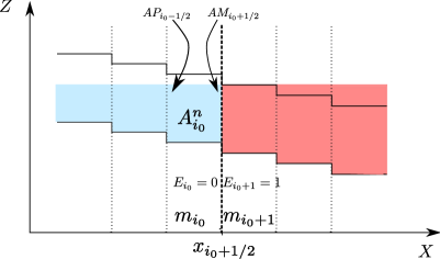
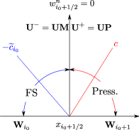
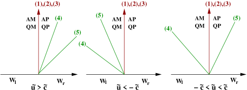
To compute the interface quantities denoted by (AM,QM)𝐴𝑀𝑄𝑀(AM,QM) for the left hand side and (AP,QP)𝐴𝑃𝑄𝑃(AP,QP) for the right hand side (see Figure 6 below), we solve the following linearised Riemann problem:

{tW+D~XW=0W={Wl=(bl,cosθl,Sl,Al,Ql)t if x<0Wr=(br,cosθr,Sr,Ar,Qr)t if x>0casessubscript𝑡W~𝐷subscript𝑋W0WcasessubscriptW𝑙superscriptsubscript𝑏𝑙subscript𝜃𝑙subscript𝑆𝑙subscript𝐴𝑙subscript𝑄𝑙𝑡 if 𝑥0subscriptW𝑟superscriptsubscript𝑏𝑟subscript𝜃𝑟subscript𝑆𝑟subscript𝐴𝑟subscript𝑄𝑟𝑡 if 𝑥0\left\{\begin{array}[]{lcl}\partial_{t}\textbf{W}+\widetilde{D}\;\partial_{X}\textbf{W}&=&0\\ \textbf{W}&=&\left\{\begin{array}[]{lcr}\textbf{W}_{l}=(b_{l},\cos\theta_{l},S_{l},A_{l},Q_{l})^{t}&\hbox{ if }&x<0\\ \textbf{W}_{r}=(b_{r},\cos\theta_{r},S_{r},A_{r},Q_{r})^{t}&\hbox{ if }&x>0\end{array}\right.\end{array}\right. (32)

with (Wl,Wr)=(Wi,Wi+1)subscriptW𝑙subscriptW𝑟subscriptW𝑖subscriptW𝑖1(\textbf{W}_{l},\textbf{W}_{r})=(\textbf{W}_{i},\textbf{W}_{i+1}) and D~=D~(Wl,Wr)=D(W~)~𝐷~𝐷subscriptW𝑙subscriptW𝑟𝐷~W\widetilde{D}=\widetilde{D}(\textbf{W}_{l},\textbf{W}_{r})=\displaystyle D(\widetilde{\textbf{W}}) where W~~W\displaystyle\widetilde{\textbf{W}} is some approximate state of the left WlsubscriptW𝑙\textbf{W}_{l} and the right WrsubscriptW𝑟\textbf{W}_{r} state.

Remark 5.2

We will see in Section 6 that the classical approximation D(W~)𝐷~WD(\widetilde{\textbf{W}}) of the Roe matrix DRoe(Wl,Wr)=01D(Wr+(1s)(WlWr))𝑑ssubscript𝐷𝑅𝑜𝑒subscriptW𝑙subscriptW𝑟superscriptsubscript01𝐷subscriptW𝑟1𝑠subscriptW𝑙subscriptW𝑟differential-d𝑠\displaystyle D_{Roe}(\textbf{W}_{l},\textbf{W}_{r})=\int_{0}^{1}D(\textbf{W}_{r}+(1-s)(\textbf{W}_{l}-\textbf{W}_{r}))\,ds defined by D~=D(W~)=D(Wl+Wr2)~𝐷𝐷~W𝐷subscriptW𝑙subscriptW𝑟2\widetilde{D}=\displaystyle D(\widetilde{\textbf{W}})=D\left(\frac{\textbf{W}_{l}+\textbf{W}_{r}}{2}\right) is not a suitable choice to preserve the still water steady state. However, we propose in Section 6 a new approximation of D~~𝐷\widetilde{D} which maintains it perfectly.

We have then W(0+,Wl,Wr)=(br,cosθr,Sr,AP,QP)tsuperscript𝑊limit-from0subscriptW𝑙subscriptW𝑟superscriptsubscript𝑏𝑟subscript𝜃𝑟subscript𝑆𝑟𝐴𝑃𝑄𝑃𝑡W^{*}(0+,\textbf{W}_{l},\textbf{W}_{r})=(b_{r},\cos\theta_{r},S_{r},AP,QP)^{t}.

The eigenvalues of the matrix D~~𝐷\widetilde{D} are λ1=0subscript𝜆10\lambda_{1}=0, λ2=0subscript𝜆20\lambda_{2}=0, λ3=0subscript𝜆30\lambda_{3}=0, λ4=u~c(W~)subscript𝜆4~𝑢𝑐~W\lambda_{4}=\widetilde{u}-c(\widetilde{\textbf{W}}), λ5=u~+c(W~)subscript𝜆5~𝑢𝑐~W\lambda_{5}=\widetilde{u}+c(\widetilde{\textbf{W}}) and the associated right eigenvectors:
r1(W~)=(c2(W~)u~200gA~0),r2(W~)=(Ψ(W~)0gA~00),r3(W~)=((S~)1000),formulae-sequencesubscript𝑟1~Wsuperscript𝑐2~Wsuperscript~𝑢200𝑔~𝐴0formulae-sequencesubscript𝑟2~WΨ~W0𝑔~𝐴00subscript𝑟3~W~𝑆1000r_{1}(\widetilde{\textbf{W}})=\left(\begin{array}[]{c}c^{2}(\widetilde{\textbf{W}})-\widetilde{u}^{2}\\ 0\\ 0\\ -g\widetilde{A}\\ 0\end{array}\right),\quad r_{2}(\widetilde{\textbf{W}})=\left(\begin{array}[]{c}\Psi(\widetilde{\textbf{W}})\\ 0\\ -g\widetilde{A}\\ 0\\ 0\end{array}\right),\quad r_{3}(\widetilde{\textbf{W}})=\left(\begin{array}[]{c}\mathcal{H}(\widetilde{S})\\ -1\\ 0\\ 0\\ 0\end{array}\right),\quad
r4(W~)=(0001u~c(W~)),r5(W~)=(0001u~+c(W~)).formulae-sequencesubscript𝑟4~W0001~𝑢𝑐~Wsubscript𝑟5~W0001~𝑢𝑐~Wr_{4}(\widetilde{\textbf{W}})=\left(\begin{array}[]{c}0\\ 0\\ 0\\ 1\\ \widetilde{u}-c(\widetilde{\textbf{W}})\end{array}\right),\quad r_{5}(\widetilde{\textbf{W}})=\left(\begin{array}[]{c}0\\ 0\\ 0\\ 1\\ \widetilde{u}+c(\widetilde{\textbf{W}})\end{array}\right).
Refer to caption
Figure 6: Solution of the Riemann problem (32). The lines (i)𝑖(i) corresponds to the characteristic lines X/t=λi𝑋𝑡subscript𝜆𝑖X/t=\lambda_{i}, for i=1,,5𝑖15i=1,\ldots,5 .

We denote P𝑃P the transition matrix associated to the right eigenvectors of D~~𝐷\widetilde{D} and P1superscript𝑃1P^{-1} its inverse. Setting [[W]]=WrWldelimited-[]delimited-[]WsubscriptW𝑟subscriptW𝑙\left[\left[\textbf{W}\right]\right]=\textbf{W}_{r}-\textbf{W}_{l}, the solution of the Riemann problem are constant states connected by shocks propagating along the characteristic lines X/t=λi𝑋𝑡subscript𝜆𝑖X/t=\lambda_{i}. The jump associated to the eigenvectors risubscript𝑟𝑖r_{i} is then equal to (P1[[W]])irisubscriptsuperscript𝑃1delimited-[]delimited-[]W𝑖subscript𝑟𝑖(P^{-1}\left[\left[\textbf{W}\right]\right])_{i}\,r_{i}. In particular, the discharge is continuous through the line X/t=0𝑋𝑡0X/t=0 since the fifth component of vectors r1subscript𝑟1r_{1}, r2subscript𝑟2r_{2} and r3subscript𝑟3r_{3} are null. It follows that the equation associated to the wet area A𝐴A remains conservative.

Thus, for instance in the subcritical case (when c(W~)<u~<c(W~)𝑐~W~𝑢𝑐~W-c(\widetilde{\textbf{W}})<\widetilde{u}<c(\widetilde{\textbf{W}})), we have:

AM=Al+gA~2c(W~)(c(W~)u~)ψlr+u~+c(W~)2c(W~)(ArAl)12c(W~)(QrQl)QM=QP=QlgA~2c(W~)ψlr+u~2c(W~)22c(W~)(ArAl)u~c(W~)2c(W~)(QrQl)AP=AM+gA~u~2c(W~)2ψlr𝐴𝑀subscript𝐴𝑙𝑔~𝐴2𝑐~W𝑐~W~𝑢superscriptsubscript𝜓𝑙𝑟~𝑢𝑐~W2𝑐~Wsubscript𝐴𝑟subscript𝐴𝑙12𝑐~Wsubscript𝑄𝑟subscript𝑄𝑙missing-subexpression𝑄𝑀𝑄𝑃subscript𝑄𝑙𝑔~𝐴2𝑐~Wsuperscriptsubscript𝜓𝑙𝑟superscript~𝑢2𝑐superscript~W22𝑐~Wsubscript𝐴𝑟subscript𝐴𝑙~𝑢𝑐~W2𝑐~Wsubscript𝑄𝑟subscript𝑄𝑙missing-subexpression𝐴𝑃𝐴𝑀𝑔~𝐴superscript~𝑢2𝑐superscript~W2superscriptsubscript𝜓𝑙𝑟\begin{array}[]{l}\displaystyle AM=A_{l}+\frac{g\,\widetilde{A}}{2\,c(\widetilde{\textbf{W}})\,(c(\widetilde{\textbf{W}})-\widetilde{u})}\,\psi_{l}^{r}+\frac{\widetilde{u}+c(\widetilde{\textbf{W}})}{2\,c(\widetilde{\textbf{W}})}\,(A_{r}-A_{l})-\frac{1}{2\,c(\widetilde{\textbf{W}})}\,(Q_{r}-Q_{l})\\ \\ \displaystyle QM=QP=Q_{l}-\frac{g\,\widetilde{A}}{2\,c(\widetilde{\textbf{W}})}\,\psi_{l}^{r}+\frac{\widetilde{u}^{2}-c(\widetilde{\textbf{W}})^{2}}{2\,c(\widetilde{\textbf{W}})}\,(A_{r}-A_{l})-\frac{\widetilde{u}-c(\widetilde{\textbf{W}})}{2\,c(\widetilde{\textbf{W}})}\,(Q_{r}-Q_{l})\\ \\ \displaystyle AP=AM+\frac{g\,\widetilde{A}}{\widetilde{u}^{2}-c(\widetilde{\textbf{W}})^{2}}\,\psi_{l}^{r}\end{array}

where ψlrsuperscriptsubscript𝜓𝑙𝑟\psi_{l}^{r} is the upwinded source term brbl+(S~)(cosθrcosθl)+Ψ(W~)(SrSl)subscript𝑏𝑟subscript𝑏𝑙~Ssubscript𝜃𝑟subscript𝜃𝑙Ψ~Wsubscript𝑆𝑟subscript𝑆𝑙b_{r}-b_{l}+\mathcal{H}(\widetilde{\mathcal{\textbf{S}}})(\cos\theta_{r}-\cos\theta_{l})+\Psi(\widetilde{\textbf{W}})(S_{r}-S_{l}).

Remark 5.3

The friction term can also be upwinded in the same way. Writing the friction term under a conservative form

XX0XK(s,S)Q(t,s)|Q(t,s)|A2(t,s)𝑑ssubscript𝑋superscriptsubscriptsubscript𝑋0𝑋𝐾𝑠S𝑄𝑡𝑠𝑄𝑡𝑠superscript𝐴2𝑡𝑠differential-d𝑠\partial_{X}\int_{X_{0}}^{X}\displaystyle\,K(s,\mathcal{\textbf{S}})\,\frac{Q(t,s)|Q(t,s)|}{A^{2}(t,s)}\,ds

(for some arbitrary X0subscript𝑋0X_{0}) allows us to write the “static” slope b𝑏b as a “dynamic” one as follows:

b+XK(s,S)Q(t,s)|Q(t,s)|A2(t,s)𝑑s𝑏subscript𝑋𝐾𝑠S𝑄𝑡𝑠𝑄𝑡𝑠superscript𝐴2𝑡𝑠differential-d𝑠b+\int_{X}\displaystyle\,K(s,\mathcal{\textbf{S}})\,\frac{Q(t,s)|Q(t,s)|}{A^{2}(t,s)}\,ds

that we denote again b𝑏b. Thus, the upwinding of the dynamic slope bi+1bisubscript𝑏𝑖1subscript𝑏𝑖b_{i+1}-b_{i} reads:

bi+1bi+XiXi+1/21Ks2{Q|Q|A2Rh(S)4/3}𝑑s+Xi+1/2Xi+11Ks2{Q|Q|A2Rh(S)4/3}𝑑ssubscript𝑏𝑖1subscript𝑏𝑖superscriptsubscriptsubscript𝑋𝑖subscript𝑋𝑖121superscriptsubscript𝐾𝑠2𝑄𝑄superscript𝐴2subscript𝑅superscriptS43differential-d𝑠superscriptsubscriptsubscript𝑋𝑖12subscript𝑋𝑖11superscriptsubscript𝐾𝑠2𝑄𝑄superscript𝐴2subscript𝑅superscriptS43differential-d𝑠b_{i+1}-b_{i}+\displaystyle\int_{X_{i}}^{X_{i+1/2}}\frac{1}{K_{s}^{2}}\left\{\frac{Q|Q|}{A^{2}R_{h}(\mathcal{\textbf{S}})^{4/3}}\right\}\,ds+\int_{X_{i+1/2}}^{X_{i+1}}\frac{1}{K_{s}^{2}}\left\{\frac{Q|Q|}{A^{2}R_{h}(\mathcal{\textbf{S}})^{4/3}}\right\}\,ds

which is equal to:

bi+1bi+(Xi+1/2Xi)Qi|Qi|Ks2Ai2Rh(Si)4/3+(Xi+1Xi+1/2)Qi+1|Qi+1|Ks2Ai+12Rh(Si+1)4/3subscript𝑏𝑖1subscript𝑏𝑖subscript𝑋𝑖12subscript𝑋𝑖subscript𝑄𝑖subscript𝑄𝑖superscriptsubscript𝐾𝑠2superscriptsubscript𝐴𝑖2subscript𝑅superscriptsubscriptS𝑖43subscript𝑋𝑖1subscript𝑋𝑖12subscript𝑄𝑖1subscript𝑄𝑖1superscriptsubscript𝐾𝑠2superscriptsubscript𝐴𝑖12subscript𝑅superscriptsubscriptS𝑖143b_{i+1}-b_{i}\displaystyle+(X_{i+1/2}-X_{i})\frac{Q_{i}|Q_{i}|}{K_{s}^{2}\,A_{i}^{2}R_{h}(\mathcal{\textbf{S}}_{i})^{4/3}}+(X_{i+1}-X_{i+1/2})\frac{Q_{i+1}|Q_{i+1}|}{K_{s}^{2}\,A_{i+1}^{2}R_{h}(\mathcal{\textbf{S}}_{i+1})^{4/3}}\,

since A𝐴A and Q𝑄Q are constant on each cells.

The terminology “dynamic” and “static” slope is used since one is (t,x)𝑡𝑥(t,x)-dependent while the other is only x𝑥x-dependent.

5.2.2 Case of transition point

In the case of a transition point, we assume that the propagation of the interface (pressurized-free surface or free surface-pressurized) has a constant speed w𝑤w during a time step. The half line x=wt𝑥𝑤𝑡x=w\,t is then the discontinuity line of D~(Wl,Wr)~𝐷subscript𝑊𝑙subscript𝑊𝑟\widetilde{D}(W_{l},W_{r}).
Let us now consider U=(A,Q)superscriptUsuperscript𝐴superscript𝑄{\textbf{U}}^{-}=(A^{-},Q^{-}) and U+=(A+,Q+)superscriptUsuperscript𝐴superscript𝑄{\textbf{U}}^{+}=(A^{+},Q^{+}) the (unknown) states respectively on the left and on the right hand side of the line x=wt𝑥𝑤𝑡x=w\,t with w=Q+QA+A𝑤superscript𝑄superscript𝑄superscript𝐴superscript𝐴\displaystyle w\leavevmode\nobreak\ =\leavevmode\nobreak\ \frac{Q^{+}\leavevmode\nobreak\ -\leavevmode\nobreak\ Q^{-}}{A^{+}\leavevmode\nobreak\ -A^{-}}. Both states UlsubscriptU𝑙{\textbf{U}}_{l} and UsuperscriptU{\textbf{U}}^{-} (resp. UrsubscriptU𝑟{\textbf{U}}_{r} and U+superscriptU{\textbf{U}}^{+}) correspond to the same type of flow. Thus it makes sense to define the averaged matrices in each zone as follows:

  • for x<wt𝑥𝑤𝑡x<w\,t, we set D~l=D~(Wl,Wr)=D(W~l)subscript~𝐷𝑙~𝐷subscriptW𝑙subscriptW𝑟𝐷subscript~W𝑙\widetilde{D}_{l}=\widetilde{D}(\textbf{W}_{l},\textbf{W}_{r})=D(\widetilde{\textbf{W}}_{l}) for some approximation W~lsubscript~W𝑙\widetilde{\textbf{W}}_{l} which connects the state WlsubscriptW𝑙\textbf{W}_{l} and WsuperscriptW\textbf{W}^{-} (see Remark 5.2).

  • for x>wt𝑥𝑤𝑡x>w\,t, we set D~r=D~(Wl,Wr)=D(W~r)subscript~𝐷𝑟~𝐷subscriptW𝑙subscriptW𝑟𝐷subscript~W𝑟\widetilde{D}_{r}=\widetilde{D}(\textbf{W}_{l},\textbf{W}_{r})=D(\widetilde{\textbf{W}}_{r}) for some approximation W~lsubscript~W𝑙\widetilde{\textbf{W}}_{l} which connects the state W+superscriptW\textbf{W}^{+} and WrsubscriptW𝑟\textbf{W}_{r} (see Remark 5.2).

Then we formally solve two Riemann problems and use the Rankine-Hugoniot jump conditions through the line x=wt𝑥𝑤𝑡x=w\,t which writes:

Q+Qsuperscript𝑄superscript𝑄\displaystyle Q^{+}-Q^{-} =\displaystyle= w(A+A)𝑤superscript𝐴superscript𝐴\displaystyle w\,(A^{+}-A^{-}) (33)
F5(A+,Q+)F5(A,Q)subscript𝐹5superscript𝐴superscript𝑄subscript𝐹5superscript𝐴superscript𝑄\displaystyle F_{5}(A^{+},Q^{+})-F_{5}(A^{-},Q^{-}) =\displaystyle= w(Q+Q)𝑤superscript𝑄superscript𝑄\displaystyle w\,(Q^{+}-Q^{-}) (34)

with F5(A,Q)=Q2A+p(X,A)subscript𝐹5𝐴𝑄superscript𝑄2𝐴𝑝𝑋𝐴F_{5}(A,Q)=\displaystyle\frac{Q^{2}}{A}+p(X,A). According to the left (UsuperscriptU{\textbf{U}}^{-}, UM) and right unknowns (U+superscriptU{\textbf{U}}^{+}, UP ) at the interface xi+1/2subscript𝑥𝑖12x_{i+1/2} and the sign of the speed w𝑤w, we have to deal with four cases:

  • pressure state propagating downstream,

  • pressure state propagating upstream,

  • free surface state propagating downstream,

  • free surface state propagating upstream.

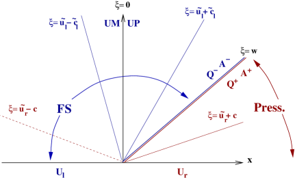
We can next consider two couples of “twin cases” : pressure state is propagating downstream (or upstream) as shown in the figure 7 and free surface state propagating downstream (or upstream) as shown in the figure 8. Moreover, for all existing transition case, the upwinded altitude term brblsubscript𝑏𝑟subscript𝑏𝑙b_{r}-b_{l} in [7] are replaced by ψlrsuperscriptsubscript𝜓𝑙𝑟\psi_{l}^{r}.

Pressure state propagating downstream:

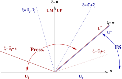
it is the case when on the left hand side of the line ξ=wt𝜉𝑤𝑡\xi=wt, we have a pressurized flow and on the right hand side we have a free surface flow: the speed w𝑤w of the transition point being positive. Following Song [28] (see also [15]), an equivalent stationary hydraulic jump must occur from a supercritical to a subcritical condition and thus the characteristics speed satisfies the inequalities:

u~r+c(W~)r<w<u~l+csubscript~𝑢𝑟𝑐subscript~W𝑟𝑤subscript~𝑢𝑙𝑐\widetilde{u}_{r}+c(\widetilde{\textbf{W}})_{r}<w<\widetilde{u}_{l}+c

where c𝑐c is the sound speed for the pressure flow, u~lsubscript~𝑢𝑙\widetilde{u}_{l}, u~rsubscript~𝑢𝑟\widetilde{u}_{r}, and c(W~)r𝑐subscript~W𝑟c(\widetilde{\textbf{W}})_{r} are defined by the same formula obtained in the case of a non transition point but according to D~lsubscript~𝐷𝑙\widetilde{D}_{l} and D~rsubscript~𝐷𝑟\widetilde{D}_{r}.

Refer to caption
Figure 7: Pressure state propagating downstream.

Therefore, only the characteristic lines drawn with solid lines are taken into account. Indeed they are related to incoming waves with respect to the corresponding space-time area <ξ<w𝜉𝑤-\infty<\xi<w. Conversely, the dotted line ξ=u~rc(W~)r𝜉subscript~𝑢𝑟𝑐subscript~W𝑟\xi=\widetilde{u}_{r}-c(\widetilde{\textbf{W}})_{r}, for instance, related to the free surface zone but drawn in the area of pressurized flow is a “ghost wave” and is not considered. Thus U+=UrsuperscriptUsubscriptU𝑟{\textbf{U}}^{+}={\textbf{U}}_{r} and UlsubscriptU𝑙{\textbf{U}}_{l}, UsuperscriptU{\textbf{U}}^{-} are connected through the jumps across the characteristics ξ=0𝜉0\xi=0 and ξ=u~lc𝜉subscript~𝑢𝑙𝑐\xi=\widetilde{u}_{l}-c. Eliminating w𝑤w in the Rankine-Hugoniot jump relations (33)-(34), we get UsuperscriptU{\textbf{U}}^{-} as the solution to the nonlinear system:

(F5(Ar,Qr)F5(A,Q))=(QrQ)2(ArA)subscript𝐹5subscript𝐴𝑟subscript𝑄𝑟subscript𝐹5superscript𝐴superscript𝑄superscriptsubscript𝑄𝑟superscript𝑄2subscript𝐴𝑟superscript𝐴\displaystyle\displaystyle(F_{5}(A_{r},Q_{r})-F_{5}(A^{-},Q^{-}))=\frac{(Q_{r}-Q^{-})^{2}}{(A_{r}-A^{-})} (35)
QQl(AAl)(u~lc)+gψlrA~lc+u~lsuperscript𝑄subscript𝑄𝑙superscript𝐴subscript𝐴𝑙subscript~𝑢𝑙𝑐𝑔subscriptsuperscript𝜓𝑟𝑙subscript~𝐴𝑙𝑐subscript~𝑢𝑙\displaystyle Q^{-}-Q_{l}-(A^{-}-A_{l})(\widetilde{u}_{l}-c)+\frac{g\psi^{r}_{l}\,\widetilde{A}_{l}}{c+\widetilde{u}_{l}} =\displaystyle= 00\displaystyle 0 (36)

Finally, we obtain :

{AP=AQM=QQP=QAM=APgA~lψlru~l2c2.cases𝐴𝑃superscript𝐴𝑄𝑀superscript𝑄𝑄𝑃superscript𝑄𝐴𝑀𝐴𝑃𝑔subscript~𝐴𝑙superscriptsubscript𝜓𝑙𝑟superscriptsubscript~𝑢𝑙2superscript𝑐2\left\{\begin{array}[]{lll}AP&=&A^{-}\\ QM&=&Q^{-}\\ QP&=&Q^{-}\\ AM&=&AP-\displaystyle\frac{g\,\widetilde{A}_{l}\,\psi_{l}^{r}}{\widetilde{u}_{l}^{2}-c^{2}}.\end{array}\right.
Free surface state propagating downstream:

on the left hand side of the line ξ=wt𝜉𝑤𝑡\xi=wt we have a free surface flow while on the right hand side, we have a pressurized flow (the speed w𝑤w of the transition point being positive). Following Song [28] again, the characteristic speed satisfies the inequalities:
u~l+c(W~)l<w<u~r+csubscript~𝑢𝑙𝑐subscript~W𝑙𝑤subscript~𝑢𝑟𝑐\widetilde{u}_{l}+c(\widetilde{\textbf{W}})_{l}<w<\widetilde{u}_{r}+c
Refer to caption
Figure 8: Free surface state propagating downstream

There are two incoming characteristic lines with respect to the free surface area <ξ<w𝜉𝑤-\infty<\xi<w (actually three with ξ=0𝜉0\xi=0) and they can connect the given left state UlsubscriptU𝑙{\textbf{U}}_{l} with any arbitrary free surface state UM. Thus only one characteristic line (ξ=u~r+c𝜉subscript~𝑢𝑟𝑐\xi=\widetilde{u}_{r}+c) gives any information (it is the equation (37) above) as an incoming characteristic line with respect to the pressurized zone w<ξ<+𝑤𝜉w<\xi<+\infty. From the jump relations through the characteristic ξ= 0𝜉 0\xi\leavevmode\nobreak\ =\leavevmode\nobreak\ 0, and after the elimination of w𝑤w in the Rankine-Hugoniot jump relations (33),(34) we get another equation, namely Equation (38) above. It remains to close the system of four unknowns (A,Q,A+,Q+)superscript𝐴superscript𝑄superscript𝐴superscript𝑄(A^{-},\,Q^{-},\,A^{+},\,Q^{+}). Firstly, we use a jump relation across the transition point (with speed w𝑤w) for the total head Ψ=u22+c2ln(AS)+g(A)cosθ+gbΨsuperscript𝑢22superscript𝑐2𝐴S𝑔𝐴𝜃𝑔𝑏\displaystyle\Psi=\frac{u^{2}}{2}+c^{2}\ln\left(\frac{A}{\mathcal{\textbf{S}}}\right)+g\,\mathcal{H}(A)\cos\theta+g\,b, from Equation (24), which writes:

Ψ+Ψ=w(u+u).superscriptΨsuperscriptΨ𝑤superscript𝑢superscript𝑢\Psi^{+}-\Psi^{-}=w\,(u^{+}-u^{-})\,.

Finally, we use the relation:

w=wpred with wpred=QrQlArAl.𝑤subscript𝑤𝑝𝑟𝑒𝑑 with subscript𝑤𝑝𝑟𝑒𝑑subscript𝑄𝑟subscript𝑄𝑙subscript𝐴𝑟subscript𝐴𝑙w=w_{pred}\,\textrm{ with }w_{pred}=\frac{Q_{r}-Q_{l}}{A_{r}-A_{l}}\,.

We have then to solve the nonlinear system:

(QrQ+)=(ArA+)(u~r+c)subscript𝑄𝑟superscript𝑄subscript𝐴𝑟superscript𝐴subscript~𝑢𝑟𝑐\displaystyle(Q_{r}-Q^{+})=(A_{r}-A^{+})\,(\widetilde{u}_{r}+c) (37)
(Q+Q)(QrQl)=(ArAl)(F2(A+,Q+)F2(A,Q))superscript𝑄superscript𝑄subscript𝑄𝑟subscript𝑄𝑙subscript𝐴𝑟subscript𝐴𝑙subscript𝐹2superscript𝐴superscript𝑄subscript𝐹2superscript𝐴superscript𝑄\displaystyle(Q^{+}-Q^{-})\,(Q_{r}-Q_{l})=(A_{r}-A_{l})\,(F_{2}(A^{+},Q^{+})-F_{2}(A^{-},Q^{-})) (38)
(Q+)22(A+)2+c2ln(A+)+gcosθ(A+)(Q)22(A)2c2ln(A)gcosθ(A)superscriptsuperscript𝑄22superscriptsuperscript𝐴2superscript𝑐2superscript𝐴𝑔𝜃superscript𝐴superscriptsuperscript𝑄22superscriptsuperscript𝐴2superscript𝑐2superscript𝐴𝑔𝜃superscript𝐴\displaystyle\frac{(Q^{+})^{2}}{2\,(A^{+})^{2}}+c^{2}\ln\left(A^{+}\right)+g\cos\theta\,\mathcal{H}(A^{+})-\frac{(Q^{-})^{2}}{2\,(A^{-})^{2}}-c^{2}\ln\left(A^{-}\right)-g\cos\theta\,\mathcal{H}(A^{-})
=QrQlArAl(Q+A+QA)absentsubscript𝑄𝑟subscript𝑄𝑙subscript𝐴𝑟subscript𝐴𝑙superscript𝑄superscript𝐴superscript𝑄superscript𝐴\displaystyle=\frac{Q_{r}-Q_{l}}{A_{r}-A_{l}}\,\left(\frac{Q^{+}}{A^{+}}-\frac{Q^{-}}{A^{-}}\right) (39)
(QrQl)(A+A)=(Q+Q)(ArAl)subscript𝑄𝑟subscript𝑄𝑙superscript𝐴superscript𝐴superscript𝑄superscript𝑄subscript𝐴𝑟subscript𝐴𝑙\displaystyle(Q_{r}-Q_{l})\,(A^{+}-A^{-})=(Q^{+}-Q^{-})\,(A_{r}-A_{l}) (40)

The states UM et UP are then obtained by the following identities:

AM=Al+gA~lψlr2c(W~)l(c(W~)lu~l)+u~l+c(W~)l2c(W~)l(AAl)12c(W~)l(QQl)AP=AM+gA~lψlru~l2c(W~)l2QM=QP=QMP=Ql+gA~lψlr2c(W~)l++u~l2c(W~)l22c(W~)l(AAl)u~lc(W~)l2c(W~)l(QQl)𝐴𝑀subscript𝐴𝑙𝑔subscript~𝐴𝑙superscriptsubscript𝜓𝑙𝑟2𝑐subscript~W𝑙𝑐subscript~W𝑙subscript~𝑢𝑙subscript~𝑢𝑙𝑐subscript~W𝑙2𝑐subscript~W𝑙superscript𝐴subscript𝐴𝑙12𝑐subscript~W𝑙superscript𝑄subscript𝑄𝑙𝐴𝑃𝐴𝑀𝑔subscript~𝐴𝑙superscriptsubscript𝜓𝑙𝑟superscriptsubscript~𝑢𝑙2𝑐superscriptsubscript~W𝑙2𝑄𝑀𝑄𝑃𝑄𝑀𝑃subscript𝑄𝑙limit-from𝑔subscript~𝐴𝑙superscriptsubscript𝜓𝑙𝑟2𝑐subscript~W𝑙superscriptsubscript~𝑢𝑙2𝑐superscriptsubscript~W𝑙22𝑐subscript~W𝑙superscript𝐴subscript𝐴𝑙subscript~𝑢𝑙𝑐subscript~W𝑙2𝑐subscript~W𝑙superscript𝑄subscript𝑄𝑙\begin{array}[]{l}\displaystyle AM=A_{l}+\frac{g\,\widetilde{A}_{l}\,\psi_{l}^{r}}{2\,c(\widetilde{\textbf{W}})_{l}(c(\widetilde{\textbf{W}})_{l}-\widetilde{u}_{l})}+\frac{\widetilde{u}_{l}+c(\widetilde{\textbf{W}})_{l}}{2\,c(\widetilde{\textbf{W}})_{l}}\,(A^{-}-A_{l})-\frac{1}{2\,c(\widetilde{\textbf{W}})_{l}}\,(Q^{-}-Q_{l})\\[14.22636pt] \displaystyle AP=AM+\frac{g\,\widetilde{A}_{l}\,\psi_{l}^{r}}{\widetilde{u}_{l}^{2}-c(\widetilde{\textbf{W}})_{l}^{2}}\\[14.22636pt] \displaystyle QM=QP=QMP=Q_{l}+\frac{g\,\widetilde{A}_{l}\,\psi_{l}^{r}}{2\,c(\widetilde{\textbf{W}})_{l}}\;+\\ \hskip 136.5733pt\displaystyle+\;\frac{\widetilde{u}_{l}^{2}-c(\widetilde{\textbf{W}})_{l}^{2}}{2\,c(\widetilde{\textbf{W}})_{l}}\,(A^{-}-A_{l})-\frac{\widetilde{u}_{l}-c(\widetilde{\textbf{W}})_{l}}{2\,c(\widetilde{\textbf{W}})_{l}}\,(Q^{-}-Q_{l})\end{array}

Finally, the update state Ain+1,Qin+1superscriptsubscript𝐴𝑖𝑛1superscriptsubscript𝑄𝑖𝑛1A_{i}^{n+1}\,,\,Q_{i}^{n+1} are obtained by the same relation as in the case of a non transition point.

Using equations (29) we update the values of Ain+1,Qin+1superscriptsubscript𝐴𝑖𝑛1superscriptsubscript𝑄𝑖𝑛1A_{i}^{n+1},\,Q_{i}^{n+1} with a standard stability condition of Courant-Friedrich-Levy controlling the time step size ΔtnΔsuperscript𝑡𝑛\Delta t^{n}.

5.2.3 Updating the state of the flow 𝑬𝑬\boldsymbol{E} in a cell.

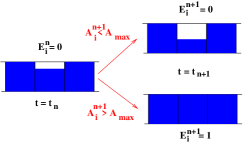
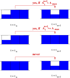
To update the state E𝐸E in the cell misubscript𝑚𝑖m_{i} (see Fig. 9), we use a discrete version of the state indicator E𝐸E defined by (19) equal to 111 for a pressurized flow and 00 otherwise. Following [7], after the computation of the wet area Ain+1superscriptsubscript𝐴𝑖𝑛1A_{i}^{n+1} we predict the state of the flow in the cell misubscript𝑚𝑖m_{i} by the following criterion:

  • \bullet

    if Ein=0superscriptsubscript𝐸𝑖𝑛0E_{i}^{n}=0 then :
    if Ain+1<Sisuperscriptsubscript𝐴𝑖𝑛1subscript𝑆𝑖A_{i}^{n+1}<S_{i} then Ein+1=0superscriptsubscript𝐸𝑖𝑛10E_{i}^{n+1}=0, else Ein+1=1superscriptsubscript𝐸𝑖𝑛11E_{i}^{n+1}=1,

  • \bullet

    if Ein=1superscriptsubscript𝐸𝑖𝑛1E_{i}^{n}=1 :
    if Ain+1Sisuperscriptsubscript𝐴𝑖𝑛1subscript𝑆𝑖A_{i}^{n+1}\geq S_{i} then Ein+1=1superscriptsubscript𝐸𝑖𝑛11E_{i}^{n+1}=1, else Ein=Ei1nEi+1nsuperscriptsubscript𝐸𝑖𝑛superscriptsubscript𝐸𝑖1𝑛superscriptsubscript𝐸𝑖1𝑛E_{i}^{n}=E_{i-1}^{n}\cdot E_{i+1}^{n}.

Indeed, if Ain+1Sisuperscriptsubscript𝐴𝑖𝑛1subscript𝑆𝑖A_{i}^{n+1}\geq S_{i} it is clear that the state of the flow in the cell misubscript𝑚𝑖m_{i} becomes pressurized, on the other hand if Ain+1<Sisuperscriptsubscript𝐴𝑖𝑛1subscript𝑆𝑖A_{i}^{n+1}<{S_{i}} in a mesh previously pressurized, we do not know a priori if the new state is free surface (ρ=ρ0𝜌subscript𝜌0\rho=\rho_{0} and the value of the wetted area is less than Sisubscript𝑆𝑖{S_{i}}) or pressurized (in depression, with ρ<ρ0𝜌subscript𝜌0\rho<\rho_{0} and the value of the wetted area is equal to Sisubscript𝑆𝑖S_{i}: see Remark 5.4 and Fig. 10).
So far as we do not take into account complex phenomena such that entrapment of air pockets or cavitation and keeping in mind that the CFL condition ensures that a transition point crosses at most one mesh at each time step, we postulate that:

  1. 1.

    if the state of the flow in the cell misubscript𝑚𝑖m_{i} is free surface at time tnsubscript𝑡𝑛t_{n}, its state at time tn+1subscript𝑡𝑛1t_{n+1} is only determined by the value of Ain+1superscriptsubscript𝐴𝑖𝑛1A_{i}^{n+1} and it cannot become in depression.

  2. 2.

    if the state of the flow in the cell misubscript𝑚𝑖m_{i} is pressurized at time tnsubscript𝑡𝑛t_{n} and if Ain+1<Sisuperscriptsubscript𝐴𝑖𝑛1subscript𝑆𝑖A_{i}^{n+1}<S_{i}, it becomes free surface if and only if at least one adjacent cell was free surface at time tnsubscript𝑡𝑛t_{n}. This is exactly the discrete version of the continuous AS𝐴S\displaystyle\frac{A}{\mathcal{\textbf{S}}} criterion in Remark 5.4 and displayed on Fig. 10.

Refer to caption Refer to caption
Figure 9: Update of the state Ein+1superscriptsubscript𝐸𝑖𝑛1E_{i}^{n+1} of the mesh misubscript𝑚𝑖m_{i}.
Remark 5.4

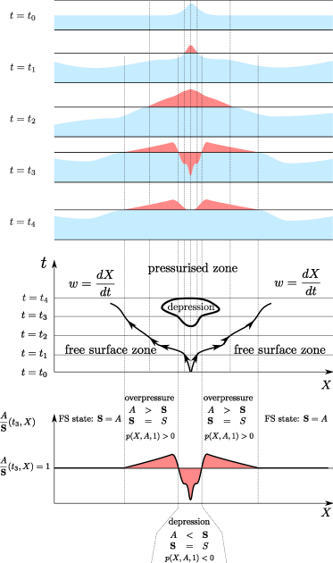
As we do not take into account complex phenomena such that entrapment of air pockets, each connected component of the pressurized area is simply connected (see Fig. 10). Moreover, for each depression area D𝐷D, its closure D¯¯𝐷\overline{D} is a strict subset of the pressurized set. It follows that when A<S𝐴𝑆A<S on each pressurized area, we observe a depression as displayed on Fig. 10. Moreover, we may also use a visual depression indicator given by the function AS𝐴S\displaystyle\frac{A}{\mathcal{\textbf{S}}}: the case S=AS𝐴\mathcal{\textbf{S}}=A corresponds to a free surface state while S>SS𝑆\mathcal{\textbf{S}}>S to an overpressure state and S<SS𝑆\mathcal{\textbf{S}}<S to a depression state. On Fig. 10, we draw the behavior of the interface speed w𝑤w in the (X,t)𝑋𝑡(X,t)-plane and the graph of the function AS𝐴S\displaystyle\frac{A}{\mathcal{\textbf{S}}} at fixed time t3subscript𝑡3t_{3}.

Refer to caption
Figure 10: AS𝐴S\displaystyle\frac{A}{\mathcal{\textbf{S}}} depression indicator.

6 Remarks on still water steady state: an exactly well balanced scheme

This section is devoted to the construction of an exactly well-balanced scheme in the sense that it maintains perfectly the still water steady states. This scheme, noted EWBS, is obtained by a suitable definition of the convection matrix.

The numerical approximation of the PFS-model (21) reads:

Ain+1superscriptsubscript𝐴𝑖𝑛1\displaystyle A_{i}^{n+1} =\displaystyle= AinΔthi(Qi+1/2nQi1/2n)superscriptsubscript𝐴𝑖𝑛Δ𝑡subscript𝑖superscriptsubscript𝑄𝑖12𝑛superscriptsubscript𝑄𝑖12𝑛\displaystyle A_{i}^{n}\displaystyle-\frac{\Delta t}{h_{i}}\left(Q_{i+1/2}^{n}-Q_{i-1/2}^{n}\right) (41)
Qin+1superscriptsubscript𝑄𝑖𝑛1\displaystyle Q_{i}^{n+1} =\displaystyle= QinΔthi(F5(AMi+1/2n,Qi+1/2n)F5(APi1/2n,Qi1/2n))superscriptsubscript𝑄𝑖𝑛Δ𝑡subscript𝑖subscript𝐹5𝐴superscriptsubscript𝑀𝑖12𝑛superscriptsubscript𝑄𝑖12𝑛subscript𝐹5𝐴superscriptsubscript𝑃𝑖12𝑛superscriptsubscript𝑄𝑖12𝑛\displaystyle Q_{i}^{n}\displaystyle-\frac{\Delta t}{h_{i}}\left(F_{5}(AM_{i+1/2}^{n},Q_{i+1/2}^{n})-F_{5}(AP_{i-1/2}^{n},Q_{i-1/2}^{n})\right) (42)

where Qi±1/2subscript𝑄plus-or-minus𝑖12Q_{i\pm 1/2} stands for QMPi±1/2𝑄𝑀subscript𝑃plus-or-minus𝑖12QMP_{i\pm 1/2} and F5(A,Q)=Q2A+c2(AS)+gI1(X,S)subscript𝐹5𝐴𝑄superscript𝑄2𝐴superscript𝑐2𝐴S𝑔subscript𝐼1𝑋S\displaystyle F_{5}(A,Q)=\frac{Q^{2}}{A}+c^{2}(A-\mathcal{\textbf{S}})+g\,I_{1}(X,\mathcal{\textbf{S}}). For instance, in the subcritical case, the interface quantities reads:

AMi+1/2n=Ain+gA~i+1/2n2c~i+1/2(c~i+1/2u~i+1/2n)ψii+1+u~i+1/2n+c~i+1/22c~i+1/2(Ai+1nAin)12c~i+1/2(Qi+1nQin)Qi+1/2n=QingA~i+1/2n2c~i+1/2ψii+1+u~i+1/2n,2c~i+1/222c~i+1/2(Ai+1nAin)u~i+1/2c~i+1/22c~i+1/2(Qi+1nQin)APi+1/2n=AMi+1/2n+gA~i+1/2nu~i+1/2n,2c~i+1/22ψii+1𝐴superscriptsubscript𝑀𝑖12𝑛superscriptsubscript𝐴𝑖𝑛𝑔superscriptsubscript~𝐴𝑖12𝑛2subscript~𝑐𝑖12subscript~𝑐𝑖12superscriptsubscript~𝑢𝑖12𝑛superscriptsubscript𝜓𝑖𝑖1missing-subexpressionmissing-subexpressionmissing-subexpressionmissing-subexpressionmissing-subexpressionsuperscriptsubscript~𝑢𝑖12𝑛subscript~𝑐𝑖122subscript~𝑐𝑖12superscriptsubscript𝐴𝑖1𝑛superscriptsubscript𝐴𝑖𝑛12subscript~𝑐𝑖12superscriptsubscript𝑄𝑖1𝑛superscriptsubscript𝑄𝑖𝑛missing-subexpressionmissing-subexpressionmissing-subexpressionsuperscriptsubscript𝑄𝑖12𝑛superscriptsubscript𝑄𝑖𝑛𝑔superscriptsubscript~𝐴𝑖12𝑛2subscript~𝑐𝑖12superscriptsubscript𝜓𝑖𝑖1superscriptsubscript~𝑢𝑖12𝑛2superscriptsubscript~𝑐𝑖1222subscript~𝑐𝑖12superscriptsubscript𝐴𝑖1𝑛superscriptsubscript𝐴𝑖𝑛missing-subexpressionmissing-subexpressionmissing-subexpressionmissing-subexpressionmissing-subexpressionsubscript~𝑢𝑖12subscript~𝑐𝑖122subscript~𝑐𝑖12superscriptsubscript𝑄𝑖1𝑛superscriptsubscript𝑄𝑖𝑛missing-subexpressionmissing-subexpressionmissing-subexpression𝐴superscriptsubscript𝑃𝑖12𝑛𝐴superscriptsubscript𝑀𝑖12𝑛𝑔superscriptsubscript~𝐴𝑖12𝑛superscriptsubscript~𝑢𝑖12𝑛2superscriptsubscript~𝑐𝑖122superscriptsubscript𝜓𝑖𝑖1\begin{array}[]{lll}\displaystyle AM_{i+1/2}^{n}&=&\displaystyle A_{i}^{n}+\frac{g\,\widetilde{A}_{i+1/2}^{n}}{2\,\widetilde{c}_{i+1/2}\,(\widetilde{c}_{i+1/2}-\widetilde{u}_{i+1/2}^{n})}\,\psi_{i}^{i+1}\\ \\ &&\displaystyle+\frac{\widetilde{u}_{i+1/2}^{n}+\widetilde{c}_{i+1/2}}{2\,\widetilde{c}_{i+1/2}}\,(A_{i+1}^{n}-A_{i}^{n})-\frac{1}{2\,\widetilde{c}_{i+1/2}}\,(Q_{i+1}^{n}-Q_{i}^{n})\\ \\ \displaystyle Q_{i+1/2}^{n}&=&\displaystyle Q_{i}^{n}-\frac{g\,\widetilde{A}_{i+1/2}^{n}}{2\,\widetilde{c}_{i+1/2}}\,\psi_{i}^{i+1}+\frac{\widetilde{u}_{i+1/2}^{n,2}-\widetilde{c}_{i+1/2}^{2}}{2\,\widetilde{c}_{i+1/2}}\,(A_{i+1}^{n}-A_{i}^{n})\\ \\ &&\displaystyle-\frac{\widetilde{u}_{i+1/2}-\widetilde{c}_{i+1/2}}{2\,\widetilde{c}_{i+1/2}}\,(Q_{i+1}^{n}-Q_{i}^{n})\\ \\ \displaystyle AP_{i+1/2}^{n}&=&\displaystyle AM_{i+1/2}^{n}+\frac{g\,\widetilde{A}_{i+1/2}^{n}}{\widetilde{u}_{i+1/2}^{n,2}-\widetilde{c}_{i+1/2}^{2}}\,\psi_{i}^{i+1}\end{array} (43)

where the upwinded source term reads:

bi+1bi+(S~i+1/2n)(cosθi+1cosθi)+Ψ(W~i+1/2n)(Si+1Si)subscript𝑏𝑖1subscript𝑏𝑖superscriptsubscript~S𝑖12𝑛subscript𝜃𝑖1subscript𝜃𝑖Ψ~W𝑖1superscript2𝑛subscript𝑆𝑖1subscript𝑆𝑖b_{i+1}-b_{i}+\mathcal{H}(\widetilde{\mathcal{\textbf{S}}}_{i+1/2}^{n})(\cos\theta_{i+1}-\cos\theta_{i})+\Psi(\widetilde{\textbf{W}}{i+1/2}^{n})(S_{i+1}-S_{i})

and c~i+1/2subscript~𝑐𝑖12\widetilde{c}_{i+1/2} stands for c(W~i+1/2n)𝑐superscriptsubscript~W𝑖12𝑛c(\widetilde{\textbf{W}}_{i+1/2}^{n}) with

W~i+1/2n=(b~i+1/2,cosθ~i+1/2,S~i+1/2,A~i+1/2n,Q~i+1/2n)superscriptsubscript~W𝑖12𝑛subscript~𝑏𝑖12subscript~𝜃𝑖12subscript~𝑆𝑖12superscriptsubscript~𝐴𝑖12𝑛superscriptsubscript~𝑄𝑖12𝑛\widetilde{\textbf{W}}_{i+1/2}^{n}=\left(\widetilde{b}_{i+1/2},\,\widetilde{\cos\theta}_{i+1/2},\,\widetilde{S}_{i+1/2},\,\widetilde{A}_{i+1/2}^{n},\,\widetilde{Q}_{i+1/2}^{n}\right)

given by

b~=bi+bi+12,cosθ~=cosθi+cosθi+12,S~=Si+Si+12,Q~i+1/2n=Qin+Qi+1n2,formulae-sequence~𝑏subscript𝑏𝑖subscript𝑏𝑖12formulae-sequence~𝜃subscript𝜃𝑖subscript𝜃𝑖12formulae-sequence~𝑆subscript𝑆𝑖subscript𝑆𝑖12superscriptsubscript~𝑄𝑖12𝑛superscriptsubscript𝑄𝑖𝑛superscriptsubscript𝑄𝑖1𝑛2\begin{array}[]{l}\displaystyle\widetilde{b}=\frac{b_{i}+b_{i+1}}{2},\,\displaystyle\widetilde{\cos\theta}=\frac{\cos\theta_{i}+\cos\theta_{i+1}}{2},\,\displaystyle\widetilde{S}=\frac{S_{i}+S_{i+1}}{2},\,\widetilde{Q}_{i+1/2}^{n}=\frac{Q_{i}^{n}+Q_{i+1}^{n}}{2},\end{array} (44)

and the approximation of A~i+1/2nsuperscriptsubscript~𝐴𝑖12𝑛\widetilde{A}_{i+1/2}^{n} to be specified.

Starting from a discrete state (Ain,Qin)superscriptsubscript𝐴𝑖𝑛superscriptsubscript𝑄𝑖𝑛(A_{i}^{n},Q_{i}^{n}) at time tnsubscript𝑡𝑛t_{n} such that:

(H)

let n𝑛n such that: ifor-all𝑖\forall i, Qin=0superscriptsubscript𝑄𝑖𝑛0Q_{i}^{n}=0 and Ainsuperscriptsubscript𝐴𝑖𝑛A_{i}^{n} satisfy the discrete still water steady state equation (according to Equation (24)):

c2ln(Ai+1nSi+1)+g(Si+1n)cosθi+1+gbi+1=c2ln(AinSi)+g(Sin)cosθi+gbi,superscript𝑐2superscriptsubscript𝐴𝑖1𝑛subscript𝑆𝑖1𝑔superscriptsubscriptS𝑖1𝑛subscript𝜃𝑖1𝑔subscript𝑏𝑖1superscript𝑐2superscriptsubscript𝐴𝑖𝑛subscript𝑆𝑖𝑔superscriptsubscriptS𝑖𝑛subscript𝜃𝑖𝑔subscript𝑏𝑖c^{2}\ln\left(\frac{A_{i+1}^{n}}{S_{i+1}}\right)+g\mathcal{H}(\mathcal{\textbf{S}}_{i+1}^{n})\cos\theta_{i+1}+gb_{i+1}=c^{2}\ln\left(\frac{A_{i}^{n}}{S_{i}}\right)+g\mathcal{H}(\mathcal{\textbf{S}}_{i}^{n})\cos\theta_{i}+gb_{i}\,, (45)

we will say that:

Definition 6.1
  1. 1.

    The numerical scheme (41-42)-(44) for some approximations of the terms A~i±1/2nsuperscriptsubscript~𝐴plus-or-minus𝑖12𝑛\widetilde{A}_{i\pm 1/2}^{n} is (kA,kQ)subscript𝑘𝐴subscript𝑘𝑄(k_{A},k_{Q}) well-balanced (also denoted by (kA,kQ)subscript𝑘𝐴subscript𝑘𝑄(k_{A},k_{Q})-WB) if:

    i,|Ain+1Ain|=O((maxihi)kA) and |Qin+1Qin|=O((maxihi)kQ),for-all𝑖superscriptsubscript𝐴𝑖𝑛1superscriptsubscript𝐴𝑖𝑛𝑂superscriptsubscript𝑖subscript𝑖subscript𝑘𝐴 and superscriptsubscript𝑄𝑖𝑛1superscriptsubscript𝑄𝑖𝑛𝑂superscriptsubscript𝑖subscript𝑖subscript𝑘𝑄\forall i,\,\begin{array}[]{l}|A_{i}^{n+1}-A_{i}^{n}|=O((\max_{i\in\mathbb{Z}}h_{i})^{k_{A}})\textrm{ and }|Q_{i}^{n+1}-Q_{i}^{n}|=O((\max_{i\in\mathbb{Z}}h_{i})^{k_{Q}})\,,\end{array}

    with kA>1subscript𝑘𝐴1k_{A}>1, kQ>1subscript𝑘𝑄1k_{Q}>1 the well-balanced order of the numerical scheme (41) and (42) respectively.

  2. 2.

    The numerical scheme (41-42)-(44) for some approximations of the terms A~i±1/2nsuperscriptsubscript~𝐴plus-or-minus𝑖12𝑛\widetilde{A}_{i\pm 1/2}^{n} is exactly well-balanced (also denoted by EWB) if:

    i,|Ain+1Ain|=0 and |Qin+1Qin|=0.for-all𝑖superscriptsubscript𝐴𝑖𝑛1superscriptsubscript𝐴𝑖𝑛0 and superscriptsubscript𝑄𝑖𝑛1superscriptsubscript𝑄𝑖𝑛0\forall i,\,\begin{array}[]{l}|A_{i}^{n+1}-A_{i}^{n}|=0\textrm{ and }|Q_{i}^{n+1}-Q_{i}^{n}|=0\,.\end{array}

We will denote by (kA,kQ)subscript𝑘𝐴subscript𝑘𝑄(k_{A},k_{Q})-WBS the (kA,kQ)subscript𝑘𝐴subscript𝑘𝑄(k_{A},k_{Q}) well-balanced scheme and EWBS the exactly well-balanced scheme.

(SF)

In the rest of this paper, we assume hi=ΔXsubscript𝑖Δ𝑋h_{i}=\Delta X constant, the radius R𝑅R and b𝑏b are given affine functions, the angle θ𝜃\theta is constant which implies that the jumps across the interface Xi+1/2subscript𝑋𝑖12X_{i+1/2}: ΔRi+1/2=Ri+1Ri=ΔRΔsubscript𝑅𝑖12subscript𝑅𝑖1subscript𝑅𝑖Δ𝑅\Delta R_{i+1/2}=R_{i+1}-R_{i}=\Delta R, Δbi+1/2=bi+1bi=ΔbΔsubscript𝑏𝑖12subscript𝑏𝑖1subscript𝑏𝑖Δ𝑏\Delta b_{i+1/2}=b_{i+1}-b_{i}=\Delta b are constant and Δcosθi+1/2Δsubscript𝜃𝑖12\Delta\cos\theta_{i+1/2} is null.

Then under this simplified framework, we show that:

Theorem 6.1
  1. 1.
    • The numerical scheme (41-42)-(44) with the classical choice

      A~i+1/2n=Ain+Ai+1n2superscriptsubscript~𝐴𝑖12𝑛superscriptsubscript𝐴𝑖𝑛superscriptsubscript𝐴𝑖1𝑛2\widetilde{A}_{i+1/2}^{n}=\displaystyle\frac{A_{i}^{n}+A_{i+1}^{n}}{2} (46)

      and non constant section S𝑆S is not well-balanced in the sense of Definition 6.1 (we have kQ=1subscript𝑘𝑄1k_{Q}=1).

    • For constant section and Z=0𝑍0Z=0, the numerical scheme (41-42)-(44) with (46) is EWB.

  2. 2.

    Under a suitable choice of A~i±1/2nsuperscriptsubscript~𝐴plus-or-minus𝑖12𝑛\widetilde{A}_{i\pm 1/2}^{n}, the numerical scheme (41-42)-(44) is EWB.

The following section deals with the numerical scheme with A~i+1/2nsuperscriptsubscript~𝐴𝑖12𝑛\widetilde{A}_{i+1/2}^{n} defined as (46) where we show the first point of Theorem 6.1. The second point is studied in Section 6.2 where a convenient definition of A~i+1/2nsuperscriptsubscript~𝐴𝑖12𝑛\widetilde{A}_{i+1/2}^{n} leads to an EWBS.

6.1 Still water steady state and the classical approximation

The simpler choice of definition for the convection matrix D(W~)𝐷~WD(\widetilde{\textbf{W}}) is the one obtained by the approximation of the mean value of the Roe matrix DRoe(Wl,Wr)=01D(Wr+(1s)(WlWr))𝑑ssubscript𝐷𝑅𝑜𝑒subscriptW𝑙subscriptW𝑟superscriptsubscript01𝐷subscriptW𝑟1𝑠subscriptW𝑙subscriptW𝑟differential-d𝑠\displaystyle D_{Roe}(\textbf{W}_{l},\textbf{W}_{r})=\int_{0}^{1}D(\textbf{W}_{r}+(1-s)(\textbf{W}_{l}-\textbf{W}_{r}))\,ds. This approximation is given by D~=D(W~)=D(Wl+Wr2)~𝐷𝐷~W𝐷subscriptW𝑙subscriptW𝑟2\widetilde{D}=\displaystyle D(\widetilde{\textbf{W}})=D\left(\frac{\textbf{W}_{l}+\textbf{W}_{r}}{2}\right) that we call “the classical approximation”. Thus, defining A~i+1/2nsuperscriptsubscript~𝐴𝑖12𝑛\widetilde{A}_{i+1/2}^{n} as follows:

A~i+1/2n=Ain+Ai+1n2superscriptsubscript~𝐴𝑖12𝑛superscriptsubscript𝐴𝑖𝑛superscriptsubscript𝐴𝑖1𝑛2\widetilde{A}_{i+1/2}^{n}=\displaystyle\frac{A_{i}^{n}+A_{i+1}^{n}}{2}\,

provides the classical approximation. But, it is not suitable to preserve the still water steady state: we will see that the numerical scheme (41-42)-(44) with (46) defines a non well-balanced scheme in the sense of Definition (6.1) since kQ=1subscript𝑘𝑄1k_{Q}=1.

To this end, let us assume (H) and (SF) at time tnsubscript𝑡𝑛t_{n}, Equations (43) read for every i𝑖i:

AMi+1/2n=Ain+gA~i+1/2n2c~i+1/22ψii+1+ΔAi+1/2n2Qi+1/2n=gA~i+1/2n2c~i+1/2ψii+1c~i+1/2ΔAi+1/2n2APi+1/2n=AMi+1/2ngA~i+1/2nc~i+1/22ψii+1.𝐴superscriptsubscript𝑀𝑖12𝑛absentsuperscriptsubscript𝐴𝑖𝑛𝑔superscriptsubscript~𝐴𝑖12𝑛2superscriptsubscript~𝑐𝑖122superscriptsubscript𝜓𝑖𝑖1Δsuperscriptsubscript𝐴𝑖12𝑛2missing-subexpressionmissing-subexpressionsuperscriptsubscript𝑄𝑖12𝑛absent𝑔superscriptsubscript~𝐴𝑖12𝑛2subscript~𝑐𝑖12superscriptsubscript𝜓𝑖𝑖1subscript~𝑐𝑖12Δsuperscriptsubscript𝐴𝑖12𝑛2missing-subexpressionmissing-subexpression𝐴superscriptsubscript𝑃𝑖12𝑛absent𝐴superscriptsubscript𝑀𝑖12𝑛𝑔superscriptsubscript~𝐴𝑖12𝑛superscriptsubscript~𝑐𝑖122superscriptsubscript𝜓𝑖𝑖1\begin{array}[]{ll}\displaystyle AM_{i+1/2}^{n}&=\displaystyle A_{i}^{n}+\frac{g\,\widetilde{A}_{i+1/2}^{n}}{2\,\widetilde{c}_{i+1/2}^{2}}\,\psi_{i}^{i+1}+\frac{\Delta A_{i+1/2}^{n}}{2}\\ \\ \displaystyle Q_{i+1/2}^{n}&=\displaystyle-\frac{g\,\widetilde{A}_{i+1/2}^{n}}{2\,\widetilde{c}_{i+1/2}}\,\psi_{i}^{i+1}-\widetilde{c}_{i+1/2}\frac{\Delta A_{i+1/2}^{n}}{2}\\ \\ \displaystyle AP_{i+1/2}^{n}&=\displaystyle AM_{i+1/2}^{n}-\frac{g\,\widetilde{A}_{i+1/2}^{n}}{\widetilde{c}_{i+1/2}^{2}}\,\psi_{i}^{i+1}\end{array}\,. (47)

Denoting Qi+1/2Qi1/2subscript𝑄𝑖12subscript𝑄𝑖12Q_{i+1/2}-Q_{i-1/2} by ΔQi+1/2Δsubscript𝑄𝑖12\Delta Q_{i+1/2}, we have:

ΔQi+1/2n=g2c~i1/2c~i+1/2{(ψi1iψii+1)c~i+1/2A~i1/2n(A~i+1/2nA~i1/2n)c~i+1/2ψii+1+(c~i+1/2c~i1/2)A~i+1/2nψii+1}+ΔAi+1/2n2(c~i1/2c~i+1/2)\begin{array}[]{lll}\Delta Q_{i+1/2}^{n}&=&\displaystyle\frac{g}{2\,\widetilde{c}_{i-1/2}\,\widetilde{c}_{i+1/2}}\Big{\{}\left(\psi_{i-1}^{i}-\psi_{i}^{i+1}\right)\widetilde{c}_{i+1/2}\,\widetilde{A}_{i-1/2}^{n}\\ &&\\ &&\displaystyle-\left(\widetilde{A}_{i+1/2}^{n}-\widetilde{A}_{i-1/2}^{n}\right)\widetilde{c}_{i+1/2}\,\psi_{i}^{i+1}\\ &&\\ &&\displaystyle+\left(\widetilde{c}_{i+1/2}-\widetilde{c}_{i-1/2}\right)\widetilde{A}_{i+1/2}^{n}\,\psi_{i}^{i+1}\Big{\}}\\ &&\\ &&\displaystyle+\frac{\Delta A_{i+1/2}^{n}}{2}\left(\widetilde{c}_{i-1/2}-\widetilde{c}_{i+1/2}\right)\end{array}

where

A~i+1/2nA~i1/2n=ΔAi+1/2nψi1iψii+1={Δb if Ei=0Δbgcosθ2ΔRc2ΔSi+1/2Si1/2Si+1/2×(ΔSi+1/2A~i1/2nΔAi+1/2nSi1/2) if Ei=1|c~i+1/2c~i1/2|{CΔX if Ei=0 ( for some constant C)=0 if Ei=1( since c~i+1/2=c~i1/2=c).\begin{array}[]{lll}\displaystyle\widetilde{A}_{i+1/2}^{n}-\widetilde{A}_{i-1/2}^{n}&=&\displaystyle\Delta A_{i+1/2}^{n}\\ &&\\ \displaystyle\psi_{i-1}^{i}-\psi_{i}^{i+1}&=&\left\{\begin{array}[]{l}\displaystyle-\Delta b\quad\textrm{ if }E_{i}=0\\ \\ \\ \displaystyle-\Delta b-\frac{g\,\cos\theta}{2}\Delta R\\ -\displaystyle\frac{c^{2}\,\Delta S_{i+1/2}}{S_{i-1/2}\,S_{i+1/2}}\\ \times\left(\Delta S_{i+1/2}\,\widetilde{A}_{i-1/2}^{n}-\Delta A_{i+1/2}^{n}\,S_{i-1/2}\right)\textrm{ if }E_{i}=1\end{array}\right.\\ &&\\ \displaystyle|\widetilde{c}_{i+1/2}-\widetilde{c}_{i-1/2}|&&\left\{\begin{array}[]{ll}\leqslant&C\Delta X\textrm{ if }E_{i}=0\,\textrm{ ( for some constant }C)\\ =&0\textrm{ if }E_{i}=1\,(\textrm{ since }\widetilde{c}_{i+1/2}=\widetilde{c}_{i-1/2}=c)\end{array}\right.\end{array}.

Denoting then

M=max(maxi(c~i+1/2A~i1/2n),maxi(c~i+1/2|ψii+1|),maxi(A~i+1/2n|ψii+1|),C)𝑀subscript𝑖subscript~𝑐𝑖12superscriptsubscript~𝐴𝑖12𝑛subscript𝑖subscript~𝑐𝑖12superscriptsubscript𝜓𝑖𝑖1subscript𝑖superscriptsubscript~𝐴𝑖12𝑛superscriptsubscript𝜓𝑖𝑖1𝐶M=\max\left(\max_{i}{\left(\widetilde{c}_{i+1/2}\,\widetilde{A}_{i-1/2}^{n}\right)},\max_{i}{\left(\widetilde{c}_{i+1/2}\,|\psi_{i}^{i+1}|\right)},\max_{i}{\left(\widetilde{A}_{i+1/2}^{n}\,|\psi_{i}^{i+1}|\right)},C\right)

and observing that

i,O(ΔR)=O(ΔSi+1/2)=O(ΔAi+1/2n)=O(ΔX)for-all𝑖𝑂Δ𝑅𝑂Δsubscript𝑆𝑖12𝑂Δsuperscriptsubscript𝐴𝑖12𝑛𝑂Δ𝑋\forall i,\,O(\Delta R)=O(\Delta S_{i+1/2})=O(\Delta A_{i+1/2}^{n})=O(\Delta X)

and

O(c~i+1/2c~i1/2)=O(Si+1/2Si1/2)=O(1),𝑂subscript~𝑐𝑖12subscript~𝑐𝑖12𝑂subscript𝑆𝑖12subscript𝑆𝑖12𝑂1O(\widetilde{c}_{i+1/2}\,\widetilde{c}_{i-1/2})=O(S_{i+1/2}\,S_{i-1/2})=O(1)\,,

we deduce:

|ΔQi+1/2n|MΔx2.Δsuperscriptsubscript𝑄𝑖12𝑛𝑀Δsuperscript𝑥2|\Delta Q_{i+1/2}^{n}|\leqslant M{\Delta x^{2}}\,.

It follows that:

|Ain+1Ain|=O(ΔX2).superscriptsubscript𝐴𝑖𝑛1superscriptsubscript𝐴𝑖𝑛𝑂Δsuperscript𝑋2|A_{i}^{n+1}-A_{i}^{n}|=O({\Delta X^{2}})\,.

Then, we denote F5(AMi+1/2n,Qi+1/2n)F5(APi1/2n,Qi1/2n)subscript𝐹5𝐴superscriptsubscript𝑀𝑖12𝑛superscriptsubscript𝑄𝑖12𝑛subscript𝐹5𝐴superscriptsubscript𝑃𝑖12𝑛superscriptsubscript𝑄𝑖12𝑛F_{5}(AM_{i+1/2}^{n},Q_{i+1/2}^{n})-F_{5}(AP_{i-1/2}^{n},Q_{i-1/2}^{n}) by ΔF=T1+T2Δ𝐹subscript𝑇1subscript𝑇2\Delta F=T_{1}+T_{2} with

T1=(AMi+1/2nAPi1/2n)(Qi+1/2n)2+AMi+1/2n((Qi+1/2n)2(Qi1/2n)2)AMi+1/2nAPi1/2nsubscript𝑇1𝐴superscriptsubscript𝑀𝑖12𝑛𝐴superscriptsubscript𝑃𝑖12𝑛superscriptsuperscriptsubscript𝑄𝑖12𝑛2𝐴superscriptsubscript𝑀𝑖12𝑛superscriptsuperscriptsubscript𝑄𝑖12𝑛2superscriptsuperscriptsubscript𝑄𝑖12𝑛2𝐴superscriptsubscript𝑀𝑖12𝑛𝐴superscriptsubscript𝑃𝑖12𝑛T_{1}=\displaystyle\frac{\left(AM_{i+1/2}^{n}-AP_{i-1/2}^{n}\right)\left(Q_{i+1/2}^{n}\right)^{2}+AM_{i+1/2}^{n}\left(\left(Q_{i+1/2}^{n}\right)^{2}-\left(Q_{i-1/2}^{n}\right)^{2}\right)}{AM_{i+1/2}^{n}\,AP_{i-1/2}^{n}}

and

T2={gcosθ(I1(Xi+1/2,,AMi+1/2n)I1(Xi+1/2,,APi1/2n)) if Ei=0c2(AMi+1/2nAPi1/2n)+c2ΔSi+1/2 if Ei=1subscript𝑇2cases𝑔𝜃subscript𝐼1subscript𝑋𝑖12𝐴superscriptsubscript𝑀𝑖12𝑛subscript𝐼1subscript𝑋𝑖12𝐴superscriptsubscript𝑃𝑖12𝑛 if subscript𝐸𝑖0missing-subexpressionmissing-subexpressionmissing-subexpressionsuperscript𝑐2𝐴superscriptsubscript𝑀𝑖12𝑛𝐴superscriptsubscript𝑃𝑖12𝑛superscript𝑐2Δsubscript𝑆𝑖12 if subscript𝐸𝑖1T_{2}=\left\{\begin{array}[]{lll}\displaystyle g\cos\theta\left(I_{1}(X_{i+1/2,},AM_{i+1/2}^{n})-I_{1}(X_{i+1/2,},AP_{i-1/2}^{n})\right)&\textrm{ if }&E_{i}=0\\ &&\\ c^{2}(AM_{i+1/2}^{n}-AP_{i-1/2}^{n})+c^{2}\Delta S_{i+1/2}&\textrm{ if }&E_{i}=1\end{array}\right.

where |(Qi+1/2n)2(Qi1/2n)2|=O(ΔX3)superscriptsuperscriptsubscript𝑄𝑖12𝑛2superscriptsuperscriptsubscript𝑄𝑖12𝑛2𝑂Δsuperscript𝑋3\displaystyle|\left(Q_{i+1/2}^{n}\right)^{2}-\left(Q_{i-1/2}^{n}\right)^{2}|=O(\Delta X^{3}) and

AMi+1/2nAPi1/2n=ΔAi+1/2n+g2(A~i+1/2nψii+1c~i+1/22+A~i1/2nψi1ic~i1/22).𝐴superscriptsubscript𝑀𝑖12𝑛𝐴superscriptsubscript𝑃𝑖12𝑛Δsuperscriptsubscript𝐴𝑖12𝑛𝑔2superscriptsubscript~𝐴𝑖12𝑛superscriptsubscript𝜓𝑖𝑖1superscriptsubscript~𝑐𝑖122superscriptsubscript~𝐴𝑖12𝑛superscriptsubscript𝜓𝑖1𝑖superscriptsubscript~𝑐𝑖122\begin{array}[]{lll}{AM_{i+1/2}^{n}-AP_{i-1/2}^{n}}&=&\displaystyle\Delta A_{i+1/2}^{n}+\frac{g}{2}\left(\frac{\widetilde{A}_{i+1/2}^{n}\psi_{i}^{i+1}}{\widetilde{c}_{i+1/2}^{2}}+\frac{\widetilde{A}_{i-1/2}^{n}\psi_{i-1}^{i}}{\widetilde{c}_{i-1/2}^{2}}\right)\end{array}\,. (48)

As the term (A~i+1/2nψii+1c~i+1/22+A~i1/2nψi1ic~i1/22)superscriptsubscript~𝐴𝑖12𝑛superscriptsubscript𝜓𝑖𝑖1superscriptsubscript~𝑐𝑖122superscriptsubscript~𝐴𝑖12𝑛superscriptsubscript𝜓𝑖1𝑖superscriptsubscript~𝑐𝑖122\displaystyle\left(\frac{\widetilde{A}_{i+1/2}^{n}\psi_{i}^{i+1}}{\widetilde{c}_{i+1/2}^{2}}+\frac{\widetilde{A}_{i-1/2}^{n}\psi_{i-1}^{i}}{\widetilde{c}_{i-1/2}^{2}}\right) is at least of order ΔXΔ𝑋\displaystyle\Delta X since

ψii+1=O(ΔX),superscriptsubscript𝜓𝑖𝑖1𝑂Δ𝑋\psi_{i}^{i+1}=O(\Delta X),

we have:

|AMi+1/2nAPi1/2n|=O(ΔX).𝐴superscriptsubscript𝑀𝑖12𝑛𝐴superscriptsubscript𝑃𝑖12𝑛𝑂Δ𝑋\displaystyle|AM_{i+1/2}^{n}-AP_{i-1/2}^{n}|=O(\Delta X)\,.

It follows that :

|Qin+1Qin|=O(ΔX).superscriptsubscript𝑄𝑖𝑛1superscriptsubscript𝑄𝑖𝑛𝑂Δ𝑋|Q_{i}^{n+1}-Q_{i}^{n}|=O({\Delta X})\,.
Remark 6.1

For constant section S𝑆S and Z=0𝑍0Z=0, it is easy to see that the numerical scheme (41-42)-(44) with (46) is EWB.

Although the scheme (41-42)-(44) with (46) have an order kQ=1subscript𝑘𝑄1k_{Q}=1 for non constant section, the still water steady state for the pressurized case is very well maintained for great value of the sonic speed c𝑐c. But it is not the case for the free surface numerical scheme (see Fig. 16 with ΔX=103Δ𝑋superscript103\Delta X=10^{-3}, b=102𝑏superscript102b=10^{-2}, uniform pipe with diameter 111). We plot in Fig. 14 and Fig. 15 a still water steady state for two values of c𝑐c for a given ΔX=1Δ𝑋1\Delta X=1 ( with b=0.9𝑏0.9b=-0.9 ): the absolute error obtained is 105superscript10510^{-5} for c=30𝑐30c=30 and 109superscript10910^{-9} for c=200𝑐200c=200. Indeed, let us consider, for the sake of simplicity, the case S=cte𝑆𝑐𝑡𝑒S=cte. At the continuous level, the still water steady state equation reads:

c2ln(A)+gRcosθ+gb=cte.superscript𝑐2𝐴𝑔𝑅𝜃𝑔𝑏𝑐𝑡𝑒c^{2}\ln\left({A}\right)+gR\cos\theta+gb=cte.

With the hypothesis (H), in particular using Equation (45), we write:

Ai+1n=Ainexp(gc2Δb).superscriptsubscript𝐴𝑖1𝑛superscriptsubscript𝐴𝑖𝑛𝑔superscript𝑐2Δ𝑏A_{i+1}^{n}=A_{i}^{n}\exp\left(-\frac{g}{c^{2}}\Delta b\right)\,.

Given ΔXΔ𝑋\Delta X, for great value of c𝑐c, we can approximate Ai+1nsuperscriptsubscript𝐴𝑖1𝑛A_{i+1}^{n} by:

Ai+1nAin(1gc2Δb).superscriptsubscript𝐴𝑖1𝑛superscriptsubscript𝐴𝑖𝑛1𝑔superscript𝑐2Δ𝑏A_{i+1}^{n}\approx A_{i}^{n}\left(1-\frac{g}{c^{2}}\Delta b\right)\,.

Then, replacing the right hand-side of Ai+1nsuperscriptsubscript𝐴𝑖1𝑛A_{i+1}^{n} in (48), we have

|AMi+1/2nAPi1/2n|=gAin|Δb|c2=O(ΔXc2).𝐴superscriptsubscript𝑀𝑖12𝑛𝐴superscriptsubscript𝑃𝑖12𝑛𝑔superscriptsubscript𝐴𝑖𝑛Δ𝑏superscript𝑐2𝑂Δ𝑋superscript𝑐2|AM_{i+1/2}^{n}-AP_{i-1/2}^{n}|=\,g\,A_{i}^{n}\frac{|\Delta b|}{c^{2}}=O\left(\frac{\Delta X}{c^{2}}\right)\,.

As we can see kQsubscript𝑘𝑄k_{Q} is always equal to 111 but the constant 1c21superscript𝑐2\displaystyle\frac{1}{c^{2}} plays the role of a smoothing term which helps the scheme (41-42)-(44) with (46) to stabilize rapidly towards the equilibrium. Physically, c𝑐c is approximatively 140014001400 (for a pressurized flow without air), thus 1c21.9 1061superscript𝑐2superscript1.9106\displaystyle\frac{1}{c^{2}}\approx 1.9\,10^{-6}. Since c(A)cmuch-less-than𝑐𝐴𝑐c(A)\ll c, this feature is not observed for the free surface numerical scheme.

6.2 An exactly well-balanced scheme

This section is devoted to the construction of an EWBS. We have seen in Subsection 6.1 that the classical approximation of with A~i±1/2nsuperscriptsubscript~𝐴plus-or-minus𝑖12𝑛\widetilde{A}_{i\pm 1/2}^{n} (46) is not appropriate to preserve the still water steady state. Thus, we have to find a suitable definition for A~i±1/2nsuperscriptsubscript~𝐴plus-or-minus𝑖12𝑛\widetilde{A}_{i\pm 1/2}^{n} to obtain an exactly well-balanced scheme. For this purpose, let us assume (SF) and start with :

at the discrete level, the still water steady state is perfectly maintained (see Fig. 11): it exists n𝑛n such that for every i𝑖i, if Qin=0superscriptsubscript𝑄𝑖𝑛0Q_{i}^{n}=0 and i,for-all𝑖\forall i,

A1:

c2ln(Ai+1nSi+1)+g(Si+1n)cosθ+gbi+1=c2ln(AinSi)+g(Sin)cosθ+gbisuperscript𝑐2superscriptsubscript𝐴𝑖1𝑛subscript𝑆𝑖1𝑔superscriptsubscriptS𝑖1𝑛𝜃𝑔subscript𝑏𝑖1superscript𝑐2superscriptsubscript𝐴𝑖𝑛subscript𝑆𝑖𝑔superscriptsubscriptS𝑖𝑛𝜃𝑔subscript𝑏𝑖\displaystyle c^{2}\ln\left(\displaystyle\frac{A_{i+1}^{n}}{S_{i+1}}\right)+g\mathcal{H}(\mathcal{\textbf{S}}_{i+1}^{n})\cos\theta+gb_{i+1}=c^{2}\ln\left(\displaystyle\frac{A_{i}^{n}}{S_{i}}\right)+g\mathcal{H}(\mathcal{\textbf{S}}_{i}^{n})\cos\theta+gb_{i},

A2:

AMi+1/2n=APi1/2n𝐴superscriptsubscript𝑀𝑖12𝑛𝐴superscriptsubscript𝑃𝑖12𝑛\displaystyle AM_{i+1/2}^{n}=AP_{i-1/2}^{n},

A3:

Qi+1/2n=Qi1/2nsuperscriptsubscript𝑄𝑖12𝑛superscriptsubscript𝑄𝑖12𝑛\displaystyle Q_{i+1/2}^{n}=Q_{i-1/2}^{n},

then, for all l>n𝑙𝑛l>n the conditions A1, A2 and A3 holds.

Refer to caption
Figure 11: Discrete representation of the mixed free surface-pressurized still water steady state at time tnsuperscript𝑡𝑛t^{n}.

The condition A2 is satisfied if and only if

AMi+1/2nAPi1/2n=ΔAi+1/2n+g2(A~i+1/2nψii+1c~i+1/22+A~i1/2nψi1ic~i1/22)=0.𝐴superscriptsubscript𝑀𝑖12𝑛𝐴superscriptsubscript𝑃𝑖12𝑛Δsuperscriptsubscript𝐴𝑖12𝑛𝑔2superscriptsubscript~𝐴𝑖12𝑛superscriptsubscript𝜓𝑖𝑖1superscriptsubscript~𝑐𝑖122superscriptsubscript~𝐴𝑖12𝑛superscriptsubscript𝜓𝑖1𝑖superscriptsubscript~𝑐𝑖1220{AM_{i+1/2}^{n}-AP_{i-1/2}^{n}}=\displaystyle\Delta A_{i+1/2}^{n}+\frac{g}{2}\left(\frac{\widetilde{A}_{i+1/2}^{n}\psi_{i}^{i+1}}{\widetilde{c}_{i+1/2}^{2}}+\frac{\widetilde{A}_{i-1/2}^{n}\psi_{i-1}^{i}}{\widetilde{c}_{i-1/2}^{2}}\right){=0}\,. (49)

The condition A3 is satisfied if and only if

ΔQi+1/2n=g2{A~i1/2nψi1ic~i1/2A~i+1/2nψii+1c~i+1/2}+ΔAi+1/2n2(c~i1/2c~i+1/2)=0.Δsuperscriptsubscript𝑄𝑖12𝑛𝑔2superscriptsubscript~𝐴𝑖12𝑛superscriptsubscript𝜓𝑖1𝑖subscript~𝑐𝑖12superscriptsubscript~𝐴𝑖12𝑛superscriptsubscript𝜓𝑖𝑖1subscript~𝑐𝑖12Δsuperscriptsubscript𝐴𝑖12𝑛2subscript~𝑐𝑖12subscript~𝑐𝑖120\Delta Q_{i+1/2}^{n}=\displaystyle\frac{g}{2}\left\{\frac{\widetilde{A}_{i-1/2}^{n}\,\psi_{i-1}^{i}}{\widetilde{c}_{i-1/2}}-\frac{\widetilde{A}_{i+1/2}^{n}\,\psi_{i}^{i+1}}{\widetilde{c}_{i+1/2}}\right\}+\frac{\Delta A_{i+1/2}^{n}}{2}\left(\widetilde{c}_{i-1/2}-\widetilde{c}_{i+1/2}\right)=0\,. (50)

The condition A1 is satisfied for pressurized flows if and only if

Ai+1n=AinSi+1Siexp(gc2(Δb+ΔRcosθ)).superscriptsubscript𝐴𝑖1𝑛superscriptsubscript𝐴𝑖𝑛subscript𝑆𝑖1subscript𝑆𝑖𝑔superscript𝑐2Δ𝑏Δ𝑅𝜃A_{i+1}^{n}=A_{i}^{n}\frac{S_{i+1}}{S_{i}}\exp\left(-\frac{g}{c^{2}}\left(\Delta b+\Delta R\cos\theta\right)\right)\,. (51)

The condition A1 is satisfied for free surface flows if and only if

hi+1n=hincosθΔbcosθ.superscriptsubscript𝑖1𝑛superscriptsubscript𝑖𝑛𝜃Δ𝑏𝜃h_{i+1}^{n}=\frac{h_{i}^{n}\cos\theta-\Delta b}{\cos\theta}\,. (52)

For circular cross-section pipe, Ai+1nsuperscriptsubscript𝐴𝑖1𝑛A_{i+1}^{n} is computed by:

Ai+1n=Ri+122(ωi+1sin(ωi+1))superscriptsubscript𝐴𝑖1𝑛superscriptsubscript𝑅𝑖122subscript𝜔𝑖1subscript𝜔𝑖1A_{i+1}^{n}=\frac{R_{i+1}^{2}}{2}\left(\omega_{i+1}-\sin(\omega_{i+1})\right) (53)

with ωi+1=2(πarccos(hi+1Ri+1))subscript𝜔𝑖12𝜋subscript𝑖1subscript𝑅𝑖1\displaystyle\omega_{i+1}=\displaystyle 2\left(\pi-\arccos\left(\frac{h_{i+1}}{R_{i+1}}\right)\right) is the angle displayed on Fig. 12.

Refer to caption
Figure 12: angle ω𝜔\omega

Thus, the discrete still water steady state is perfectly maintained if and only if, (A~i1/2n,A~i+1/2n)superscriptsubscript~𝐴𝑖12𝑛superscriptsubscript~𝐴𝑖12𝑛(\widetilde{A}_{i-1/2}^{n},\widetilde{A}_{i+1/2}^{n}) is the solution of the non-linear system:

{0=ΔAi+1/2n+g2(A~i+1/2nψii+1c~i+1/22+A~i1/2nψi1ic~i1/22)0=g2{A~i1/2nψi1ic~i1/2A~i+1/2nψii+1c~i+1/2}+ΔAi+1/2n2(c~i1/2c~i+1/2)cases0Δsuperscriptsubscript𝐴𝑖12𝑛𝑔2superscriptsubscript~𝐴𝑖12𝑛superscriptsubscript𝜓𝑖𝑖1superscriptsubscript~𝑐𝑖122superscriptsubscript~𝐴𝑖12𝑛superscriptsubscript𝜓𝑖1𝑖superscriptsubscript~𝑐𝑖122missing-subexpressionmissing-subexpressionmissing-subexpression0𝑔2superscriptsubscript~𝐴𝑖12𝑛superscriptsubscript𝜓𝑖1𝑖subscript~𝑐𝑖12superscriptsubscript~𝐴𝑖12𝑛superscriptsubscript𝜓𝑖𝑖1subscript~𝑐𝑖12Δsuperscriptsubscript𝐴𝑖12𝑛2subscript~𝑐𝑖12subscript~𝑐𝑖12\left\{\begin{array}[]{lll}0&=&\displaystyle\Delta A_{i+1/2}^{n}+\frac{g}{2}\left(\frac{\widetilde{A}_{i+1/2}^{n}\psi_{i}^{i+1}}{\widetilde{c}_{i+1/2}^{2}}+\frac{\widetilde{A}_{i-1/2}^{n}\psi_{i-1}^{i}}{\widetilde{c}_{i-1/2}^{2}}\right)\\ &&\\ 0&=&\displaystyle\frac{g}{2}\left\{\frac{\widetilde{A}_{i-1/2}^{n}\,\psi_{i-1}^{i}}{\widetilde{c}_{i-1/2}}-\frac{\widetilde{A}_{i+1/2}^{n}\,\psi_{i}^{i+1}}{\widetilde{c}_{i+1/2}}\right\}+\frac{\Delta A_{i+1/2}^{n}}{2}\left(\widetilde{c}_{i-1/2}-\widetilde{c}_{i+1/2}\right)\end{array}\right. (54)

where we have replaced the expression of Ai+1nsuperscriptsubscript𝐴𝑖1𝑛A_{i+1}^{n} in (49-50) by (51) for pressurized by (52) for free surface flows:

ΔAi+1/2n={Ain(Si+1Siexp(gc2(Δb+ΔRcosθ))1) if Ei=0(hincosθΔbcosθ) if Ei=0.Δsuperscriptsubscript𝐴𝑖12𝑛casessuperscriptsubscript𝐴𝑖𝑛subscript𝑆𝑖1subscript𝑆𝑖𝑔superscript𝑐2Δ𝑏Δ𝑅𝜃1 if subscript𝐸𝑖0superscriptsubscript𝑖𝑛𝜃Δ𝑏𝜃 if subscript𝐸𝑖0\Delta A_{i+1/2}^{n}=\left\{\begin{array}[]{lll}\displaystyle A_{i}^{n}\left(\frac{S_{i+1}}{S_{i}}\exp\left(-\frac{g}{c^{2}}\left(\Delta b+\Delta R\cos\theta\right)\right)-1\right)&\textrm{ if }&E_{i}=0\\ \displaystyle\mathcal{F}\left(\frac{h_{i}^{n}\cos\theta-\Delta b}{\cos\theta}\right)&\textrm{ if }&E_{i}=0\end{array}\right.\,.

with :h(h)=A:maps-to𝐴\mathcal{F}:h\mapsto\mathcal{F}(h)=A. For circular pipe, \mathcal{F} is given by (53).

Finally, the numerical scheme (41-42)-(44) with A~i±1/2nsuperscriptsubscript~𝐴plus-or-minus𝑖12𝑛\widetilde{A}_{i\pm 1/2}^{n} as the solution of the non linear system (54) defines an exactly well-balanced scheme.

For uniform pipe and pressurized flow, the previous system simply writes:

{ΔAi+1/2n+gΔZ2c2(A~i+1/2n+A~i1/2n)=0A~i+1/2n=A~i1/2n.casesΔsuperscriptsubscript𝐴𝑖12𝑛𝑔Δ𝑍2superscript𝑐2superscriptsubscript~𝐴𝑖12𝑛superscriptsubscript~𝐴𝑖12𝑛0missing-subexpressionmissing-subexpressionmissing-subexpressionsuperscriptsubscript~𝐴𝑖12𝑛superscriptsubscript~𝐴𝑖12𝑛\left\{\begin{array}[]{lll}\displaystyle\Delta A_{i+1/2}^{n}+\frac{g\,\Delta Z}{2\,c^{2}}\left(\widetilde{A}_{i+1/2}^{n}+\widetilde{A}_{i-1/2}^{n}\right)&=&0\\ &&\\ \widetilde{A}_{i+1/2}^{n}&=&\widetilde{A}_{i-1/2}^{n}\end{array}\right.\,.

The solution is easily obtained by:

A~i+1/2n=c2gΔAi+1/2nΔb=c2gAin(exp(gc2Δb)1)Δb.superscriptsubscript~𝐴𝑖12𝑛superscript𝑐2𝑔Δsuperscriptsubscript𝐴𝑖12𝑛Δ𝑏superscript𝑐2𝑔superscriptsubscript𝐴𝑖𝑛𝑔superscript𝑐2Δ𝑏1Δ𝑏\widetilde{A}_{i+1/2}^{n}=-\frac{c^{2}}{g}\frac{\Delta A_{i+1/2}^{n}}{\Delta b}=\displaystyle-\frac{c^{2}}{g}\frac{A_{i}^{n}\left(\exp\left(\displaystyle-\frac{g}{c^{2}}\Delta b\right)-1\right)}{\Delta b}\,. (55)

Let us also remark that using the relation Ain=Ai+1nexp(gc2Δb)superscriptsubscript𝐴𝑖𝑛superscriptsubscript𝐴𝑖1𝑛𝑔superscript𝑐2Δ𝑏A_{i}^{n}=A_{i+1}^{n}\exp\left(\displaystyle\frac{g}{c^{2}}\Delta b\right), we have:

A~i+1/2n=c2gΔAi+1/2nΔb=c2gAi+1n(1exp(gc2Δb))Δb.superscriptsubscript~𝐴𝑖12𝑛superscript𝑐2𝑔Δsuperscriptsubscript𝐴𝑖12𝑛Δ𝑏superscript𝑐2𝑔superscriptsubscript𝐴𝑖1𝑛1𝑔superscript𝑐2Δ𝑏Δ𝑏\widetilde{A}_{i+1/2}^{n}=-\frac{c^{2}}{g}\frac{\Delta A_{i+1/2}^{n}}{\Delta b}=\displaystyle-\frac{c^{2}}{g}\frac{A_{i+1}^{n}\left(1-\exp\left(\displaystyle\frac{g}{c^{2}}\Delta b\right)\right)}{\Delta b}\,. (56)

It follows that A~i+1/2nsuperscriptsubscript~𝐴𝑖12𝑛\widetilde{A}_{i+1/2}^{n} can be expressed as the mean value of (55) and (56) as follows:

A~i+1/2n=c2gΔb{Ai+1n(1exp(gc2Δb))+Ain(exp(gc2Δb)1)2}.superscriptsubscript~𝐴𝑖12𝑛superscript𝑐2𝑔Δ𝑏superscriptsubscript𝐴𝑖1𝑛1𝑔superscript𝑐2Δ𝑏superscriptsubscript𝐴𝑖𝑛𝑔superscript𝑐2Δ𝑏12\widetilde{A}_{i+1/2}^{n}=\displaystyle-\frac{c^{2}}{g\,\Delta b}\left\{\frac{A_{i+1}^{n}\left(1-\exp\left(\displaystyle\frac{g}{c^{2}}\Delta b\right)\right)+A_{i}^{n}\left(\exp\left(\displaystyle-\frac{g}{c^{2}}\Delta b\right)-1\right)}{2}\right\}\,.

For small ΔXΔ𝑋\Delta X, we have

A~i+1/2nAin+Ai+1n2.superscriptsubscript~𝐴𝑖12𝑛superscriptsubscript𝐴𝑖𝑛superscriptsubscript𝐴𝑖1𝑛2\widetilde{A}_{i+1/2}^{n}\approx\frac{A_{i}^{n}+A_{i+1}^{n}}{2}\,.

It follows that the scheme (41-42)-(44) with (46) is the zero order approximation of the solution given by the EWBS.

The same analysis shows that the free surface numerical scheme with (46) is also the zero order approximation of the solution given by the EWBS.

On Fig. 14, Fig. 15, Fig. 16, we display the still water steady pressurized and free surface state computed by the EWBS and the scheme with the approximation (46). The steady state with the EWBS is numerically well preserved while as pointed out before (see Subsection 6.1) the classical approach is not convenient.

We also display an unsteady simulation on Fig. 17 where the results of the two methods are very well reproduced.

6.3 Remarks concerning mixed still water steady state

The previous sections deals with the well-balanced property of the numerical scheme (41-42)-(44) for free surface and pressurized flows. To use the well-balanced scheme developed in Subsections (6.1) and (6.2), we start from the discrete representation of a mixed still water steady state (as displayed on Fig. 11). Assume that there exists i0subscript𝑖0i_{0} such that all cells misubscript𝑚𝑖m_{i} on the left hand side of the interface xi0+1/2subscript𝑥subscript𝑖012x_{i_{0}+1/2} are free surface while the other are pressurized:

{Ei=0 if ii0Ei=1 if i>i0.casessubscript𝐸𝑖0 if 𝑖subscript𝑖0subscript𝐸𝑖1 if 𝑖subscript𝑖0\left\{\begin{array}[]{lll}E_{i}=0&\textrm{ if }&i\leqslant i_{0}\\ E_{i}=1&\textrm{ if }&i>i_{0}\end{array}\,.\right.

The interface xi0+1/2subscript𝑥subscript𝑖012x_{i_{0}+1/2} is such that the speed of propagation of the interface is null: wi0+1/2n=Qi+1nQinAi+1nAin=0superscriptsubscript𝑤subscript𝑖012𝑛superscriptsubscript𝑄𝑖1𝑛superscriptsubscript𝑄𝑖𝑛superscriptsubscript𝐴𝑖1𝑛superscriptsubscript𝐴𝑖𝑛0w_{i_{0}+1/2}^{n}=\displaystyle\frac{Q_{i+1}^{n}-Q_{i}^{n}}{A_{i+1}^{n}-A_{i}^{n}}=0 (see Fig. 13). Therefore, UM=UUMsuperscriptU{\textbf{UM}}={\textbf{U}}^{-} and UP=U+UPsuperscriptU{\textbf{UP}}={\textbf{U}}^{+}.

Refer to caption
Figure 13: Mixed free surface-pressurized still water steady state

For example on Fig. 13, we apply the free surface numerical scheme on the left hand side of the interface and the pressurized one on the right cells . As the EWBS preserves the pressurized and free surface still water steady state, it also preserves the mixed still water steady state.

7 Numerical tests

The numerical validation for pipes with constant section and slope has been previously studied by two of the authors in [7, 8] and thus are not presented in this paper. Since experimental data for mixed flows in any pipe are not available, we focus on the behavior of our method for several circular cross-section contracting and expanding pipe. Notice that, the equivalent pipe method is not relevant for the mixed flows as pointed out by [1, 29, 30] for instance.

The mixed flow case is numerically performed on a water hammer test. Starting from an horizontal free surface still water steady state, the water hammer occurs immediately after the increase of the upstream piezometric head while the downstream discharge is set to 00. The prescribed hydrograph produces a travelling wave which produces a pressurized state propagating from upstream to downstream end. Physically an trapped air pocket may appear: it is not taken into account in the PFS-model. Actually, the trapped air pockets vanish or move; some parts of these pockets undergo condensation/vaporisation and others parts move and lead to a two phase flow. Consequently the sound speed decreases. As our model does not take into account these phenomena, the value of c𝑐c is assumed to be constant. Moreover we should have to deal with the entrapment of air bubbles which have a non negligible effect (see [19, 27] for instance).

The numerical experiments are performed in the case of a 100100100 m𝑚m long closed circular pipe at altitude b0=1msubscript𝑏01𝑚b_{0}=1\,m with 00 slope which corresponds to the elevation and slope of the main pipe axis (we have Z=b(X)=0,Xformulae-sequence𝑍𝑏𝑋0for-all𝑋Z=b(X)=0,\,\forall X). The Manning roughness coefficient is 1/Ks=0.012s/m1/31subscript𝐾𝑠0.012𝑠superscript𝑚131/K_{s}=0.012\;s/m^{1/3}. The simulation starts from a steady state as a free surface flow with a discharge Q=0m3/s𝑄0superscript𝑚3𝑠Q=0\;m^{3}/s. The upstream boundary condition is a prescribed hydrograph (see Fig. 19) while the downstream discharge is kept constant to 0m3/s0superscript𝑚3𝑠0\,m^{3}/s (as displayed on Fig. 19). We compare then the results obtained for uniform, contracting an expanding pipes. For each test, the parameters are the same except the downstream diameter: the upstream diameter is kept constant to D=1m𝐷1𝑚D=1\,m. The contracting pipe is chosen for D=0.6m𝐷0.6𝑚D=0.6\,m and the expanding one for D=1.4m𝐷1.4𝑚D=1.4\,m (where D𝐷D denotes the downstream diameter). Let us recall that the zero water level corresponds to the main pipe axis. The piezometric head is defined as z+p𝑧𝑝z+p:

{p=2R+c2(ρρ0)ρ0g if the flow is pressurizedp=h the water height if the flow is free surfacecases𝑝2𝑅superscript𝑐2𝜌subscript𝜌0subscript𝜌0𝑔 if the flow is pressurized𝑝 the water height if the flow is free surface\displaystyle\left\{\begin{array}[]{l}\displaystyle p=2R+\frac{c^{2}\,(\rho-\rho_{0})}{\rho_{0}\,g}\mbox{ if the flow is pressurized}\\ p=h\mbox{ the water height if the flow is free surface}\end{array}\right.

Results are then represented on Fig. 20. The sudden raise of the upstream piezometric level produces a pressurized state with a travelling wave. A water hammer is then observed since the downstream discharge is null. A careful analysis of the flow which is performed by the variable E𝐸E or equivalently by AS𝐴S\displaystyle\frac{A}{\mathcal{\textbf{S}}} (see Remark 5.4 and Fig. 10) shows that after this transition point, the flow is pressurized but in depression which starts approximatively at time 19s19𝑠19s for the contracting pipe, 24s24𝑠24s for the uniform pipe and 28s28𝑠28s for the expanding one. We display the piezometric line for different times around the depression time (see Fig. 21) and also the graph of the function AS𝐴S\displaystyle\frac{A}{\mathcal{\textbf{S}}} which confirm that the observed times correspond exactly to a depression state for each pipes (see Fig. 22).

We also observe a little smoothing effect and absorption due to the first order discretisation type.

8 Conclusion

We have derived a free surface and a pressurized model which have been coupled using a common set of variables and a suitable pressure law. We have thus obtained a mathematical model for unsteady mixed flows in non uniform water pipes, that we have called PFS-model. This model takes into account the local perturbation of the section and of the slope.

The PFS model is numerically solved by a VFRoe scheme using the interfacial upwind to include the source terms into the numerical fluxes. We have shown that the classical approximation of the convection matrix (the Roe matrix approximation) is not suitable to preserve the still water steady state (except for the pressurized case where the value of c𝑐c helps the scheme to maintain this state). Moreover, we have proposed a manner to obtain an exactly well-balanced scheme.

As mentioned in [7] this numerical method with the classical approximation of the convection matrix, for constant section, reproduces correctly laboratory tests for uniform pipes and can deal with multiple points of transition between the two types of flows. As pointed out before, due to the lack of experimental data for non uniform pipes, we have only shown the behavior of the piezometric line which seems reasonable (at less no major difference was observed).

As a well-known feature on approximate Godunov scheme, the upwinding of the source terms may introduce stationary waves with a vanishing denominator when critical flows occurs i.e. uc𝑢𝑐u\approx c. Moreover, in its actual form, the presented numerical scheme is not able to deal with drying and flooding area. Nevertheless, it may be possible to introduce a cut-off function to avoid division by zero for each problems: critical stationary waves, drying area and flooding area. But it is not the better choice that we can propose, since, truncation of the wet area induces a loss of water mass leading to the non-conservativity of the mass. Nevertheless, at the present time, we are interested in a mathematical kinetic formulation of the PFS model and the construction of a numerical kinetic scheme that avoids all these drawbacks [6].

The next step is to take into account the air entrainment which may have non negligible effects on the behaviour of the piezometric head. A first approach has been derived in the case of perfect fluid and perfect gas modelised as a bilayer model based on the PFS-model [5].

Aknowlegments: The authors wish to thank the two referees for their careful reading of the first version of the article and useful remarks.

References

  • [1] A. Adamkowski. Analysis of transient flow in pipes with expanding or contracting sections. ASME J. of Fluid Engineering, 125:716–722, 2003.
  • [2] B. Alvarez-Samaniego and D. Lannes. Large time existence for 3D water-waves and asymptotics. Invent. Math., 171(3):485–541, 2008.
  • [3] F. Bouchut, E.D. Fernández-Nieto, A. Mangeney, and P.-Y. Lagrée. On new erosion models of Savage-Hutter type for avalanches. Acta Mech., 199:181–208, 2008.
  • [4] F. Bouchut, A. Mangeney-Castelnau, B. Perthame, and J.-P.Vilotte. A new model of Saint Venant and Savage-Hutter type for gravity driven shallow water flows. C. R. Math. Acad. Sci. Paris, 336(6):531–536, 2003.
  • [5] C. Bourdarias, M. Ersoy, and S. Gerbi. Air entrainment in transient flows in closed water pipes: a two-layer approach. submitted, available at http://arxiv.org/abs/0910.0334, 2009.
  • [6] C. Bourdarias, M. Ersoy, and S. Gerbi. A model for unsteady mixed flows in non uniform closed water pipes: a Full Kinetic Approach. In preparation, 2009.
  • [7] C. Bourdarias and S. Gerbi. A finite volume scheme for a model coupling free surface and pressurized flows in pipes. J. Comp. Appl. Math., 209(1):109–131, 2007.
  • [8] C. Bourdarias and S. Gerbi. A conservative model for unsteady flows in deformable closed pipe and its implicit second order finite volume discretisation. Computers & Fluids, 37:1225–1237, 2008.
  • [9] C. Bourdarias, S. Gerbi, and M. Gisclon. A kinetic formulation for a model coupling free surface and pressurized flows in closed pipes. J. Comp. Appl. Math., 218(2):522–531, 2008.
  • [10] M. Boutounet, L. Chupin, P. Noble, and J-P. Vila. Shallow water viscous flows for arbitrary topopgraphy. Commun. Math. Sci., 6(1):29–55, 2008.
  • [11] D. Bresch and P. Noble. Mathematical justification of a shallow water model. Methods Appl. Anal., 14(2):87–117, 2007.
  • [12] T. Buffard, T. Gallouët, and J.M. Hérard. A sequel to a rough Godunov scheme. application to real gases. Computers and Fluids, 31:813–847, 2000.
  • [13] H. Capart, X. Sillen, and Y. Zech. Numerical and experimental water transients in sewer pipes. Journal of Hydraulic Research, 35(5):659–672, 1997.
  • [14] Nguyen Trieu Dong. Sur une méthode numérique de calcul des écoulements non permanents soit à surface libre, soit en charge, soit partiellement à surface libre et partiellement en charge. La Houille Blanche, 2:149–158, 1990.
  • [15] Musandji Fuamba. Contribution on transient flow modelling in storm sewers. Journal of Hydraulic Research, 40(6):685–693, 2002.
  • [16] T. Gallouët, J.M. Hérard, and N. Seguin. Some approximate Godunov schemes to compute shallow-water equations with topography. Computers and Fluids, 32:479–513, 2003.
  • [17] J.-F. Gerbeau and B. Perthame. Derivation of viscous Saint-Venant system for laminar shallow water; numerical validation. Discrete Cont. Dyn. Syst. Ser. B, 1(1):89–102, 2001.
  • [18] J.M. Greenberg and A.Y. LeRoux. A well balanced scheme for the numerical processing of source terms in hyperbolic equation. SIAM J. Numer. Anal., 33(1):1–16, 1996.
  • [19] M.A. Hamam and A. McCorquodale. Transient conditions in the transition from gravity to surcharged sewer flow. Can. J. Civ. Eng., 9:189–196, 1982.
  • [20] F. Kerger, P. Archambeau, S. Erpicum, B. J. Dewals, and M. Pirotton. Improved one-dimensional numerical simulation of transient mixed flow in water pipe. In Proceedings of 4th Int. Conf. on Advanced Computational Methods in Engineering Liege, Belgium., 2008.
  • [21] F. Kerger, P. Archambeau, S. Erpicum, B. J. Dewals, and M. Pirotton. Numerical simulation of highly transient mixed flow in sewer system. La Houille Blanche, 2009. to appear.
  • [22] F. Kerger, S. Detrembleur, P. Archambeau, S. Erpicum, B. J. Dewals, and M. Pirotton. An experimental analysis of effects induced by moving bodies in shallow water. In Proceedings of 2nd Int. Junior Researcher and Engineer Workshop on Hydraulic Structures, Pisa, Italy., 2008.
  • [23] C-D. Levermore, M. Oliver, and Edriss S. Titi. Global well-posedness for models of shallow water in a basin with a varying bottom. Indiana University Mathematics Journal., 45(2), 1996.
  • [24] F. Marche. Derivation of a new two-dimensional viscous shallow water model with varying topography, bottom friction and capillary effects. European Journal of Mechanic. B, Fluids, 26(1):49–63, 2007.
  • [25] P.L. Roe. Some contributions to the modelling of discontinuous flow. In B. E. Engquist, S. Osher, and R. C. J. Somerville, editors, Large-scale computations in fluid mechanics. Part 2. Proceedings of the fifteenth AMS-SIAM summer seminar on applied mathematics held at Scripps Institution of Oceanography, La Jolla, Calif., June 27-July 8, 1983, volume 22 of Lectures in Applied Mathematics, pages 163–193. American Mathematical Society, 1985.
  • [26] A. Y. Le Roux and M. N. Le Roux. Convergence d’un schéma à profils stationnaires pour les équations quasi linéaires du premier ordre avec termes sources. C. R. Acad. Sci., Sér. I, Math. 333(7):703–706, 2001.
  • [27] C.S.S. Song. Two-phase flow hydraulic transient model for storm sewer systems. In Second international conference on pressure surges, pages 17–34, Bedford, England, 1976. BHRA Fluid engineering.
  • [28] C.S.S. Song, J.A. Cardle, and K.S. Leung. Transient mixed-flow models for storm sewers. Journal of Hydraulic Engineering, ASCE, 109(11):1487–1503, 1983.
  • [29] V.L. Streeter, E.B. Wylie, and K.W. Bedford. Fluid Mechanics. McGraw-Hill, 1998.
  • [30] E.B. Wylie and V.L. Streeter. Fluid Transients. McGraw-Hill, New York, 1978.
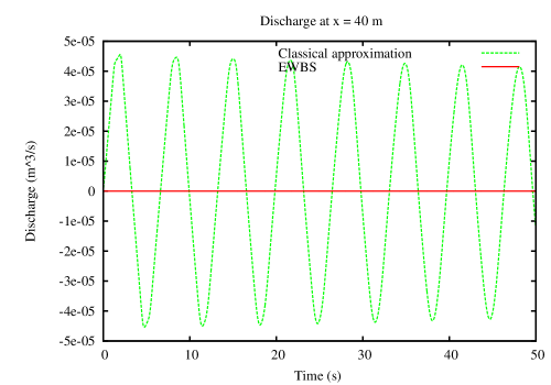
Refer to caption
Refer to caption
Figure 14: The numerical scheme (41-42)-(44) with (46) and the EWBS for pressurized still water steady state with c=30𝑐30c=30.
Refer to caption
Refer to caption
Figure 15: The numerical scheme (41-42)-(44) with (46) and the EWBS for pressurized still water steady state with c=200𝑐200c=200.
Refer to caption
Refer to caption
Figure 16: The numerical scheme (41-42)-(44) with (46) and the EWBS for free surface still water steady state.
Refer to caption
Refer to caption
Figure 17: A non stationary test to compare the EWBS and the numerical scheme (41-42)-(44) with (46).
Refer to caption
Refer to caption
Refer to caption
Figure 18: Initial still water steady state for contracting, uniform and expanding pipes .
Refer to caption
Refer to caption
Figure 19: Boundary conditions.
Refer to caption
Refer to caption
Figure 20: Piezometric head and discharge at X=50m𝑋50𝑚X=50m.
Refer to caption
Refer to caption
Refer to caption
Figure 21: Observation of the depression localised approximatively at time t=19.117𝑡19.117t=19.117 (contracting pipe), t=24.075𝑡24.075t=24.075 (uniform pipe) and t=28.395𝑡28.395t=28.395 (expanding pipe).
Refer to caption
Refer to caption
Refer to caption
Figure 22: Observation of the depression localised approximatively at time t=19.117𝑡19.117t=19.117 (contracting pipe), t=24.075𝑡24.075t=24.075 (uniform pipe) and t=28.395𝑡28.395t=28.395 (expanding pipe).