Extremum complexity in the monodimensional ideal gas:
the piecewise uniform density distribution approximation

Abstract

In this work, it is suggested that the extremum complexity distribution of a high dimensional dynamical system can be interpreted as a piecewise uniform distribution in the phase space of its accessible states. When these distributions are expressed as one–particle distribution functions, this leads to piecewise exponential functions. It seems plausible to use these distributions in some systems out of equilibrium, thus greatly simplifying their description. In particular, here we study an isolated ideal monodimensional gas far from equilibrium that presents an energy distribution formed by two non–overlapping Gaussian distribution functions. This is demonstrated by numerical simulations. Also, some previous laboratory experiments with granular systems seem to display this kind of distributions.

I Introduction

In general, a variational formulation can be established for the principles that govern the physical world. Thus, the technique of extremizing a particular physical quantity has been traditionally very useful for solving many different problems. A notable example in the thermodynamics field is that of the maximum entropy principle, which basically states that a system under constraints (i.e. isolated) will evolve by monotonically increasing its entropy with time and will reach equilibrium at its maximum achievable entropy Jaynes (1957). This principle is valuable in two distinct ways. First, it unambiguously provides a way to determine the state of equilibrium, which for the case of an isolated system will be that of the equiprobability among the accessible states. This property is useful within the field of equilibrium thermodynamics or thermostatics. And secondly, it gives a definite direction in which the system will evolve toward equilibrium, which is effectively an arrow of time. This property is valuable by restricting the evolution of systems to those of ever growing entropy. It also tells us that the entropy is equivalent to a stretched or compressed time axis. In summary, the latter property is useful for thermodynamics in its broader sense, that is, for systems out of equilibrium.

Recently Calbet and Lopez-Ruiz (2007), the extremum complexity assumption has been proven valuable for greatly restricting the possible accessible states of an isolated system far away from equilibrium. It states that isolated systems out of equilibrium can be simplified by assuming equiprobability among some of the total accessible states and zero probability of occupation for the rest of them. Equivalently, we can say that the probability density function of the system is approximated by a piecewise uniform distribution among the accessible states. The spirit of this hypothesis is that in some isolated systems local complexity can arise despite its increase in entropy. A typical example being life which can be maintained in an isolated system as long as internal resources last.

In this paper, we will justify this hypothesis and will extend this concept applied to the monodimensional ideal gas. It will be shown that for some isolated systems relaxing towards equilibrium, it is a good approximation to assume that the system follows a series of states with extremum complexity, the extremum complexity path. The usefulness of this idea resides in simplifying the dynamics of the system by allowing to describe very complex systems with just a few parameters. Advancing some of our results, in section VI, the state of a monodimensional ideal gas far from equilibrium with $10,000$ particles will be explained by a reduced set of only nine variables. We shall also see in section VIII how some experiments with granular systems Kudrolli and Henry (2000) also seem to show an extremum complexity distribution.

In section II, the equivalence between extremum complexity states and piecewise uniform distributions will be presented. A justification for this assumption will be explained in section III. These concepts will be applied to the monodimensional ideal gas in section IV. The extremum complexity distribution and approximations in this monodimensional ideal gas are shown in section V and VI, where the assumption of extremum complexity will be shown to greatly simplify the dynamics of the system. Results of the numerical simulation of the monodimensional ideal gas are presented in section VII. Some distributions found in experiments with granular systems Kudrolli and Henry (2000) also seem to be extremum complexity ones. This is suggested in section VIII. Finally, a discussion of the results is given in section IX.

II Extremum complexity distribution is a piecewise uniform density distribution

When an isolated system relaxes towards equilibrium, it does so by monotonically increasing its entropy. In this context, the entropy is equivalent to a stretched time axis. In some particular cases Calbet and Lopez-Ruiz (2001, 2007), the extremum complexity hypothesis can be also assumed, which means that we have a supplementary constraint, namely, the isolated system prefers to relax toward equilibrium by approaching or following the extremum complexity path Calbet and Lopez-Ruiz (2001).

The so called LMC complexity $C$ given by Lopez-Ruiz et al. (1995) is defined as

$$C=H\cdot D,$$ (1)

where the disequilibrium, $D$ is defined in Lopez-Ruiz et al. (1995) as the distance of the system state to the microcanonical equilibrium distribution, the equiprobability,

$$D=\sum_{i=1}^{N}(f_{i}-1/N)^{2},$$ (2)

and $H$ is the normalized entropy,

$$H=-(1/\ln N)\sum_{i=1}^{N}f_{i}\ln f_{i},$$ (3)

where $N$ is the number of accessible states and $f_{i}$, with $i=1,2,\dots N$, is the probability of occurrence of particular state $i$ of the system. Other authors have proposed different definitions for the disequilibrium, which are claimed to exhibit a more appropriate behavior than the original definition for some particular applications. See Martin et al. Martin et al. (2006) for a comprehensive list of them. At any rate, the extremum complexity distribution happens to be identical for almost all of these LMC-like complexities Martin et al. (2006).

The extremum complexity distribution can be calculated by finding the complexity extrema for a given entropy, $H$, using Lagrange multipliers Calbet and Lopez-Ruiz (2001). Table 1 shows the resulting distribution functions. The extremum distribution function is graphically shown for all accessible states of the system in Fig. 1. It can be subdivided in two components, one with the maximum probability, which will be referred as “king distribution”, and another one with the rest of the non-zero probabilities, which will be named “people distribution”. An important aspect to note is that both distributions are uniform within a certain domain of the phase space and zero everywhere else. They are effectively piecewise uniform distributions. In this respect, extremum complexity distributions are equivalent to piecewise uniform ones.

Table 1: Probability values, $f_{j}$, that give a maximum complexity, $C$, for a given entropy, $H$. $f_{k}$ is the king distribution and $f_{p}$ is the people distribution.

Number of states with $\displaystyle f_{j}$	$\displaystyle f_{j}$	Range of $\displaystyle f_{j}$
$\displaystyle 1$	$f_{k}=f_{\rm max}$	$\displaystyle 1/N\ \ldots\ 1$
$\displaystyle N-1$	$f_{p}=(1-f_{\rm max})/(N-1)$	$\displaystyle 0\ \ldots\ 1/N$

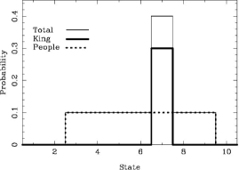
Figure 1: Microcanonical extremum complexity distribution derived in Ref. Calbet and Lopez-Ruiz (2001) for $N=8$. It is the sum of the king (thick solid line and $f_{K}$ with $f_{k}=0.3$ in Table 1) and the people, or equiprobability for non-zero states, distribution (dotted line and $f_{P}$ with $f_{p}=0.1$ in Table 1).

III Evolution of a piecewise uniform distribution

There are many systems where the initial probability distribution function is effectively a piecewise uniform function. A clear example is the monodimensional ideal gas with $N$ particles as shown in Calbet and Lopez-Ruiz (2007) and in section IV. In this example two very energetic particles are introduced into a gas previously in equilibrium. The picture of the system, just before the introduction of the extreme energetic particles, is that of a distribution function in which the accessible states of the system form a uniformly distributed hypersphere in the $(N-2)$-dimensional phase space. Right after we introduce the high energetic particles, the whole accessible space is blown up extremely into a much bigger hypersphere in the final $N$-dimensional phase space. The original $N-2$ particles that where in equilibrium will still occupy the $(N-2)$-dimensional uniformly distributed hypersphere, that is, a subspace of the much bigger $N$-dimensional hypersphere. The 2 energetic particles will occupy a place in the $N$-dimensional hypersphere with very high momentum. Because of this, globally, a very big part of the accessible N-dimensional hypersphere will have zero probability of being occupied, or in other words, the global distribution could be approximated by one or more (two for this example of the monodimensional gas) piecewise uniform distribution functions.

After this initial moment, the distribution function will be modified as the system relaxes towards equilibrium until it reaches the equiprobability within the $N$-dimensional hypersphere. The evolution of the system between this initial state and the equilibrium one will depend on the particular example studied. Still, we can sketch how the system will evolve by using an important property of Frobenius-Perron operators Mackey (1992). If we define $S$ as the nonsingular transformation governing the evolution of a dynamical system in phase space $x$, $f$ as the probability density function and $P$ as the operator to calculate the evolution of $f$, then this property states that for every set $A$, $Pf(x)=0$ for all elements $x\in A$ if and only if $f(x)=0$ for all $x\in S^{-1}(A)$. In practical terms this means that if the system is initially with many states with zero probability of occurrence, then the system will evolve by keeping many of the regions of phase space with zero probability. The rest of the non-zero probability states can be assigned a constant probability as a first approximation. In other words, the system can be approximated as evolving from one piecewise uniform density function to another one, always remaining close to the extremum complexity state.

To illustrate this concept, we will look at the density function of a system that evolves by following the tent map. The tent map is governed by the following equations,

$$S(x)=\quad\begin{cases}2x&,0\leq x<\frac{1}{2}\\ 2(1-x)&,\frac{1}{2}\leq x\leq 1\end{cases}$$ (4)

Its density function evolution can be easily calculated Mackey (1992) and is given by

$$Pf(x)=\frac{1}{2}\left[f(\frac{1}{2}x)+f(1-\frac{1}{2}x)\right]$$ (5)

The stationary density function for this system is the equiprobability. If we now initialize the system with a piecewise uniform density function, we will verify that the density distribution is transformed from one piecewise uniform function to approximately another one in such a way that the region with zero probability keeps getting smaller (see Fig. 2). At the final stage, the zero probability region disappears and the system is in an equiprobable distribution.

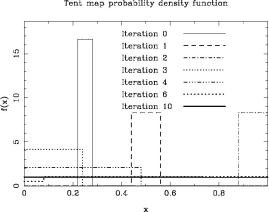
Figure 2: Time evolution of an initially piecewise uniform distribution function for the tent map. The distribution function tends to stay, in a first approximation, as a piecewise uniform distribution.

Following this illustration and thanks to the above mentioned property of the Frobenius-Perron operators, it is to be expected that a system which has the equiprobability as its equilibrium distribution and is initialized with a function similar to a piecewise uniform distribution, will evolve approximately following subsequent piecewise uniform distributions until it reaches the equiprobability.

IV The monodimensional ideal gas far from equilibrium

In the simulations, the gas is initially, at time $t=0$, in equilibrium. Its one particle momentum distribution is described by a Gaussian or Maxwell–Boltzmann function. At this point, two new extremely energetic particles are introduced into the gas, forcing the gas into a far from equilibrium state. The system is kept isolated from then on. It eventually relaxes again toward equilibrium showing asymptotically another Gaussian distribution. The relaxation towards equilibrium of this isolated monodimensional gas follows the extremum complexity path.

The evolution of the system can be approximated by two functions, the people and the king distribution, which are piecewise uniform on the accessible states of the system Calbet and Lopez-Ruiz (2007). A double Gaussian distribution will result when we transform these N-dimensional distributions into one particle momentum ones (see Fig. 4).

In more detail, and using arbitrary units from now on, the gas consisted of $10,000$ point-like particles colliding with each other elastically. The particles were positioned with alternating masses of $1$ and $2$ on regular intervals on a linear space $10,000$ units long. The system has no boundaries, i.e., the last particle in this linear space was allowed to collide with the first one, in a way similar to a set of rods on a circular ring. Two distinct masses in the system were used because a monodimensional gas can thermalize only if its constituent particles have at least two different masses. Initially $9998$ particles were given initial conditions following a Gaussian distribution with mean zero velocity and a mean energy of $1/2$, giving a total mean energy for the system of nearly $5,000$. These particles where then allowed to undergo $20$ million collisions in order for the system to reach the initial state of equilibrium, i.e., a Gaussian distribution. After that, at time $t=0$, two extremely energetic particles of mass $1$ and $2$ are introduced at two neighboring points, such that the total system has zero momentum and several different final energies of $E=10,000$, $75,000$, $150,000$ and $1,500,000$. The system then undergoes another $20$ million collisions to reach again the equilibrium Gaussian distribution. We record the time evolution of the one-dimensional momentum distribution in Fig. 4, where the square of the generalized particle momentum is given by the variable

$$p^{2}_{i}\equiv P^{2}_{i}/m_{i},$$ (6)

with $P_{i}$ and $m_{i}$ the momentum and mass of particle $i$ respectively. The theoretical extremum complexity or piecewise uniform distributions (derived below) for this system is approximated by two non-overlapping Gaussian distributions and is also fitted as solid lines in Fig. 4. Let us remark that the system stays in this double Gaussian, the extremum complexity distribution, during a large part of its out of equilibrium state. The two clearly visible slopes of Fig. 4 are related with the two different widths associated with both Gaussian distributions. As the system approaches equilibrium, both Gaussian distributions merge into one. More details of the numerical simulations are deferred to section VII.

V Extremum Complexity distribution of an isolated monodimensional ideal gas

In Calbet and Lopez-Ruiz (2007), we showed a different derivation of the extremum complexity distribution to the one shown here, both obtaining the same results. We will make our study inside the N-dimensional phase space constituted by the generalized momentums. We will also define an m-dimensional sphere as one located in an m-dimensional space.

Since initially $N-2$ particles are in equilibrium, they will be located on an $N-2$ dimensional hypersphere within the $N$ dimensional phase space. This will be our people distribution. The remaining 2 high energetic particles will be located on a 2-dimensional hypersphere embedded in the global N-dimensional phase space. This will conform the king distribution.

As the system evolves in time, the particles of the people distribution will slowly migrate to the king distribution. Following the extremum complexity approximation, we will assume both distributions are piecewise uniform ones, being uniform where they are non-zero.

Each one of the particles will be assumed to be either in the people or king distribution. The distributions will be separated by a particular value of the generalized momentum $p_{0}$. If the absolute value of the generalized momentum is below (above) $p_{0}$ then the particle will belong to the people (king) distribution. Denoting by $n_{p}$, $n_{k}$ the number of particles and $e_{p}$ and $e_{k}$ the half–variances of the Gaussian distributions in the people and the king distributions, respectively , then the particles of the people distribution, with absolute generalized momentums below $p_{0}$, are distributed uniformly over the $n_{p}$-dimensional sphere of radius $\sqrt{2n_{p}e_{p}}$. The rest of the particles, forming the king distribution, with absolute generalized momentums above $p_{0}$, will be distributed uniformly on an $n_{k}$-dimensional sphere of radius $\sqrt{2n_{k}e_{k}}$. The cartesian product of these hyperspheres will be embedded on the $N$-dimensional hypersphere within the complete $N$-dimensional phase space.

We can now calculate the one–particle momentum distribution by integrating both distributions in $N$–dimensional phase space into just one dimension. This is done in Appendix A. Combining both one–particle momentum distributions, the complete distribution function for the monodimensional ideal gas far away from equilibrium can be written as,

$$f(p)=\quad\begin{cases}K_{p}\;\exp(-p^{2}/4e_{p}),&|p|<p_{0}\\ K_{k}\;\exp(-p^{2}/4e_{k}),&|p|\geq p_{0}\end{cases}$$ (7)

with $K_{p}$ and $K_{k}$ normalization constants of the distribution function, such that,

$$\int_{0}^{p_{0}}f(p)\;{\rm d}p=n_{p}$$ (8)

$$\int_{p_{0}}^{\infty}f(p)\;{\rm d}p=n_{k},$$ (9)

which must satisfy the conservation of particles by maintaining $N$ constant,

$$N=n_{p}+n_{k}.$$ (10)

Separating the people and the king function we can now define,

$$f_{p}(p)\equiv K_{p}\;\exp(-p^{2}/4e_{p})$$

$$f_{k}(p)\equiv K_{k}\;\exp(-p^{2}/4e_{k}).$$ (11)

We will also require the distribution function to be continuous,

$$f_{p}(p_{0})=f_{k}(p_{0}).$$ (12)

VI Extremum complexity approximation equations in the monodimensional gas

We can now define the total energies, $E_{p}$ and $E_{k}$, and the mean energy per particle, $\overline{e_{p}}$ and $\overline{e_{k}}$, of the people and king distribution such that the total energy of the system, $E$, is conserved,

$$E_{p}=n_{p}\overline{e_{p}}$$

$$E_{k}=n_{k}\overline{e_{k}}$$

$$E=E_{p}+E_{k}.$$ (13)

We can combine the distribution functions of Eq. (V), the conservation principles discussed and the concepts shown in section V to obtain the extremum complexity approximation equations of the monodimensional gas,

$$n_{p}=\int_{0}^{p_{0}}K_{p}\;\exp(-p^{2}/4e_{p})\;{\rm d}p$$ (14)

$$n_{k}=\int_{p_{0}}^{\infty}K_{k}\;\exp(-p^{2}/4e_{k})\;{\rm d}p$$ (15)

$$N=n_{p}+n_{k}$$ (16)

$$K_{p}\exp(-p_{0}^{2}/4e_{p})=K_{k}\;\exp(-p_{0}^{2}/4e_{k})$$ (17)

$$E=n_{p}\overline{e_{p}}+n_{k}\overline{e_{k}}$$ (18)

$$\overline{e_{p}}=\dfrac{\int_{0}^{p_{0}}\dfrac{p^{2}}{2}\exp(-p^{2}/4e_{p}){\rm d}p}{\int_{0}^{p_{0}}\exp(-p^{2}/4e_{p})\;{\rm d}p}$$ (19)

$$\overline{e_{k}}=\dfrac{\int_{p_{0}}^{\infty}\dfrac{p^{2}}{2}\exp(-p^{2}/4e_{k}){\rm d}p}{\int_{p_{0}}^{\infty}\exp(-p^{2}/4e_{k})\;{\rm d}p},$$ (20)

where Eqs. (14) and (15) are the expressions of the number of particles in each distribution, Eq. (16) is the conservation of particles, Eq. (17) is the continuity of the distribution function, Eq. (18) is the conservation of energy and Eqs. (19) and (20) are the definitions of the mean energy per particle.

We are thus left with seven equations and nine unknowns, $n_{p}$, $K_{p}$, $e_{p}$, $\overline{e_{p}}$, $n_{k}$, $K_{k}$, $e_{k}$, $\overline{e_{k}}$ and $p_{0}$, having simplified the monodimensional ideal gas description enormously.

We need two more equations to completely describe the system. These will be obtained from the Boltzmann integro–differential equation. Let us first consider the two particle collisions within the monodimensional gas, which should conserve energy and momentum. If the generalized momentums before the collisions are $(p,p_{1})$ and the ones after the collision are $(p^{\prime},p^{\prime}_{1})$, and the collisions are elastic then they must satisfy,

$$p^{\prime}=\dfrac{(m-m_{1})}{(m+m_{1})}p+\dfrac{2\sqrt{m}\sqrt{m_{1}}}{(m+m_{1})}p_{1}$$ (21)

$$p^{\prime}_{1}=\dfrac{2\sqrt{m}\sqrt{m_{1}}}{(m+m_{1})}p-\dfrac{(m-m_{1})}{(m+m_{1})}p_{1}$$ (22)

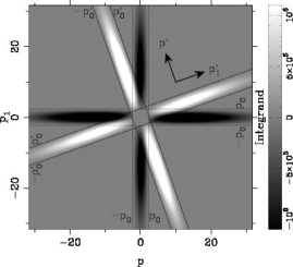
Figure 3: Numerical values of the integrand of the Boltzmann equation for the monodimensional gas (Eq. (VI)).

The net effect of a collision is a rotation and swapping of the generalized momentums on the $(p,p_{1})$ space. This is shown in Fig. 3. The angle of rotation $\theta$ is given by

$$\cos(\theta)=\frac{2\sqrt{m}\sqrt{m_{1}}}{m+m_{1}}.$$ (23)

Let us now obtain the Boltzmann integro–differential equation for our particular gas. Due to setting the gas by alternating two different masses in physical space, for a given generalized momentum, $p$, there can correspond particles with two different masses, $m_{0}$ and $m_{*}$. Each one of these particles will collide with another one with an alternative mass. The Boltzmann equation for this particular monodimensional gas is,

$$\dfrac{\partial f(p)}{\partial t}= \int\left[\dfrac{1}{2}\left|\dfrac{p_{1}}{\sqrt{m_{*}}}-\dfrac{p}{\sqrt{m_{0}}}\right|+\dfrac{1}{2}\left|\dfrac{p_{1}}{\sqrt{m_{0}}}-\dfrac{p}{\sqrt{m_{*}}}\right|\right]\centerdot$$

$$(f(p^{\prime}_{1})f(p^{\prime})-f(p)f(p_{1}))\;{\rm d}p_{1}$$ (24)

Using the extremum complexity equations (Eqs. (V)) we can plot the different values of the integrand of the Boltzmann equation to find the most significant ones. This is shown in Fig. 3. It can be seen that collisions in which two particles are both in the people (or king) distribution before and after the collision do not alter the distribution function giving an integrand of zero.

We shall now concentrate on the evolution of the people distribution function. As we can see from Fig. 3 the greatest contribution to the integrand of the Boltzmann equation will come from collisions where initially we have one particle belonging to the people distribution and the other one to the king distribution and after the collision they both belong to the king distribution. The original Boltzmann equation, Eq. (VI), is then simplified to,

$$\dfrac{\partial f_{p}(p)}{\partial t}\cong\int_{p_{0}}^{\infty}\left[\dfrac{1}{2}\left|\dfrac{p_{1}}{\sqrt{m_{*}}}-\dfrac{p}{\sqrt{m_{0}}}\right|+\dfrac{1}{2}\left|\dfrac{p_{1}}{\sqrt{m_{0}}}-\dfrac{p}{\sqrt{m_{*}}}\right|\right]\centerdot$$

$$\left(K_{k}{\rm e}^{-p^{\prime 2}_{1}/4e_{k}}\;K_{k}{\rm e}^{-p^{\prime 2}/4e_{k}}-K_{p}{\rm e}^{-p^{2}/4e_{p}}\;K_{k}{\rm e}^{-p^{2}_{1}/4e_{k}}\right)\;{\rm d}p_{1}$$ (25)

Rearranging terms and using the conservation of energy, $p^{2}+p_{1}^{2}=p^{\prime 2}+p^{\prime 2}_{1}$, we are left with,

$$\dfrac{\partial f_{p}(p)}{\partial t}=\left(K_{k}{\rm e}^{-p^{2}/4e_{k}}-K_{p}{\rm e}^{-p^{2}/4e_{p}}\right)\centerdot$$

$$\int_{p_{0}}^{\infty}\left[\dfrac{1}{2}\left|\dfrac{p_{1}}{\sqrt{m_{*}}}-\dfrac{p}{\sqrt{m_{0}}}\right|+\dfrac{1}{2}\left|\dfrac{p_{1}}{\sqrt{m_{0}}}-\dfrac{p}{\sqrt{m_{*}}}\right|\right]\centerdot$$

$$K_{k}\exp(-p_{1}^{2}/4e_{k})\;{\rm d}p_{1}$$ (26)

Taking into account that the momentum from the king distribution, $p_{1}$, is usually much larger than the one from the people distribution, $p$, we can approximately say that

$$\dfrac{1}{2}\left[\left|\dfrac{p_{1}}{\sqrt{m_{*}}}-\dfrac{p}{\sqrt{m_{0}}}\right|+\dfrac{1}{2}\left|\dfrac{p_{1}}{\sqrt{m_{0}}}-\dfrac{p}{\sqrt{m_{*}}}\right|\right]\approx$$

$$\dfrac{1}{2}\left[\left|\dfrac{p_{1}}{\sqrt{m_{*}}}\right|+\dfrac{1}{2}\left|\dfrac{p_{1}}{\sqrt{m_{0}}}\right|\right].$$ (27)

The probabilities of the king distribution are much lower than the ones from the people distribution, which allows us to simplify,

$$\left(K_{k}{\rm e}^{-p^{2}/4e_{k}}-K_{p}{\rm e}^{-p^{2}/4e_{p}}\right)\approx$$

$$-K_{p}\exp(-p^{2}/4e_{p}).$$ (28)

Combining these two approximations gives us the final evolution equation for the people distribution,

$$\dfrac{\partial f_{p}(p)}{\partial t}\approx-f_{p}(p)\;\mu_{k},$$ (29)

where,

$$\mu_{k}=\int_{p_{0}}^{\infty}\left[\dfrac{1}{2}\left|\dfrac{p_{1}}{\sqrt{m_{*}}}\right|+\dfrac{1}{2}\left|\dfrac{p_{1}}{\sqrt{m_{0}}}\right|\right]K_{k}{\rm e}^{-p_{1}^{2}/4e_{k}}\;{\rm d}p_{1}.$$ (30)

Note that $\mu_{k}$ is similar to an average of the absolute value of the velocity times the number of particles in the king distribution.

To transform Eq. (29) into the variables used in the extremum complexity approximation, we can integrate it for values of $p$ between $0$ and $p_{0}$ to obtain,

$$\dfrac{\partial n_{p}}{\partial t}\simeq-n_{p}\;\mu_{k}.$$ (31)

We can obtain an expression for the people energy by multiplying both sides of Eq. (29) by $p^{2}/2$ and integrating again within the limits of the people distribution,

$$\dfrac{\partial E_{p}}{\partial t}\simeq-E_{p}\;\mu_{k}.$$ (32)

Combining Eq. (31) and (32) we can obtain the relationship of the mean energy per particle of the people distribution,

$$\dfrac{\partial\overline{e_{p}}}{\partial t}\approx 0.$$ (33)

Adding Eqs. (31) and (33) to the previous set of equations (Eqs. (14) to (20)) completes the set by having a total of nine equations for nine unknowns.

VII Results of the numerical simulations

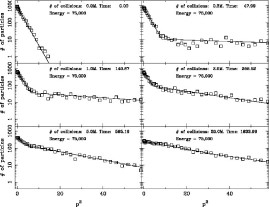
Figure 7: Same as Fig. 4 but with a total constant energy of $75,000$.

Numerical simulations have been carried out for $10,000$ particles located in a space $10,000$ units long with an energy of about $5,000$ before the introduction of the extremely energetic particles. This energy was distributed following a Gaussian distribution in generalized momentum space. To make sure they were really in an equilibrium state before the experiment started they were further collided 20 million times. After this, two high energetic particles are introduced in the system giving a total momentum of $0$. Results for total constant energies of $10,000$, $75,000$, $150,000$ and $1,500,000$ after the introduction of the energetic particles are shown in Figs. 8, 7, 4 and 6.

For each one of these experiments, the generalized momentum histogram has been fitted to two non-overlapping Gaussians. There will be cases where this fit will not be easy to achieve, namely when predominantly only one Gaussian distribution is present. This happens at the beginning, where we mainly have the initial Maxwell-Boltzmann distribution, and at the end of the experiment, where we mainly have the final equilibrium Gaussian distribution. The case with an energy of $10,000$ is a particularly difficult one to separate at all times due to the small relative difference between the two Gaussians. This difficulty will manifest itself as less well determined parameters exhibiting a higher “noise”. Because of this, only figures of the fitted parameters with a total energy of $1,500,000$ are shown. Results for the other energies are similar albeit showing a higher noise. Note that this noise could be lowered if the algorithm to fit the two Gaussians to the experimental points were improved.

Other numerical simulations (not shown here) have been performed where the initial pair of high energetic particles where introduced in different places in the monodimensional gas. They all exhibit the same behavior as the ones shown here.

In Fig. 4 the results for the numerical simulations with a total constant energy of $150,000$ after the introduction of the very energetic particles are shown. The axes of the graph are the generalized momentum squared and the logarithm of the generalized momentum. The two non-overlapping Gaussian distributions are clearly shown. Fig. 5 shows the same histograms but in direct scales in both axes. Again both non-overlapping Gaussian distributions are clearly seen.

In Fig. 6, 7 and 8 results with the exactly the same initial conditions (initial energy of about $5,000$) but with different energies given to the extremely energetic particles providing a total constant energy of $1,500,000$ , $75,000$ and $10,000$ respectively. In all cases the system behaves following a double Gaussian or maximum complexity distribution. The case with a total energy of $10,000$ is worth mentioning. This system takes a much longer time to relax to equilibrium than the others. It is also very difficult to separate both Gaussian distributions exhibiting a very high noise in the derived parameters. It may well be that in fact the system is not following the two Gaussian distribution, but it is difficult to tell (Fig. 8).

The evolution of the system in phase space for a total energy of 1,500,000 is shown in Fig. 9. We can see how the gas forms clusters of higher and lower velocity particles. Some high energetic particles are located within the low velocity clusters.

The number of particles in the people and king distribution is shown in Fig. 10 (energy of $1,500,000$). The difficulty in separating both Gaussian distributions is clearly seen as “noise” in the figure close to $t=0$. At higher times (right part of the graph) the noise slowly increases until it is so high that the results at not valuable any more. Both population numbers show an exponential evolution in time. The solid line for $n_{p}$ is an exponential fit to the simulations and it can be derived from Eq. (14). This is better seen in Fig. 11 where the logarithm of the people distribution population is shown. The deviation of the exponential behavior at the right side of the graph could be caused by the above mentioned “noise”. Again, the solid line is a numerical fit to the simulations.

The modelled parameters $e_{p}$ and $e_{k}$ parameters for the people and king distribution using Eqs. (33) and (18) as a function of time are shown in Figs. 12 and 13 respectively. These parameters are equivalent to the sigma of the Gaussian distributions. The mean energy per particle for the people distribution, $\overline{e_{p}}$, which is represented as a solid line, remains approximately constant as expected (Eq. (33)).

In Fig. 14 the momentum value, $p_{0}$, separating the people and king distribution as a function of time is shown. The solid line is the theoretical value obtained with Eqs. (14) to (20) and Eqs. (31) and (33).

Finally, in Fig. 15 the histograms for different times are shown for a total constant energy of $1,500,000$. In this case, the solid lines have been obtained with the experimental fit of $n_{p}$ (Fig. 11) and Eqs. (14) to (20) and Eqs. (31) and (33). The fit could be improved (not shown in this paper) if we take second order terms in Eqs. (31) and (33).

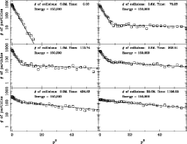
Figure 4: Numerical simulations of an isolated monodimensional ideal gas where two highly energetic particles are introduced into a thermalised state with an initial energy of about $5,000$, giving a total constant energy of $150,000$. The logarithm of the generalized momentum histogram (squares) is shown as a function of $p^{2}$ for different times. Two non–overlapping Gaussian functions are fitted to the histogram and are shown as a solid line.

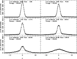
Figure 5: Numerical simulations of an isolated monodimensional ideal gas where two highly energetic particles are introduced into a thermalized state with an initial energy of about $5,000$, giving a total constant energy of $150,000$. The direct generalized momentum histogram (squares) is shown for different times. Two non–overlapping Gaussian functions are fitted to the histogram and are shown as a solid line.

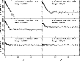
Figure 6: Same as Fig. 4 but with a total constant energy of $1,500,000$.

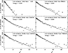
Figure 8: Same as Fig. 4 but with a total constant energy of $10,000$.

8

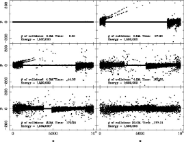
Figure 9: Monodimensional ideal gas particles in phase space. The $x$ axis is the regular spatial coordinate and the vertical axis is the generalized momentum one.

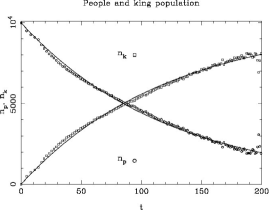
Figure 10: Number of particles in the people (circles) and king (squares) distributions as a function of time for the case with a total constant energy of $1,500,000$. The solid line for $n_{p}$ is an exponential fit to the simulations, it can be derived from Eq. (14).

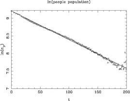
Figure 11: Logarithm of the number of particles in the people distribution as a function of time for the case with a total constant energy of $1,500,000$.

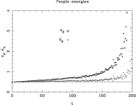
Figure 12: Two times sigma of the Gaussian people distribution, $e_{p}$ (see Eq. (V)), (circles) and mean people distribution energy per particle, $\overline{e_{p}}$, (pluses) as a function of time for the case with a total constant energy of $1,500,000$. The solid line is the mean energy per particle for the people distribution, $\overline{e_{p}}$, which remains approximately constant as expected (Eq. (33).

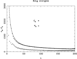
Figure 13: Two times sigma of the Gaussian king distribution, $e_{k}$ (see Eq. (V)), (squares) and mean king distribution energy per particle, $\overline{e_{k}}$, (crosses) as a function of time for the case with a total constant energy of $1,500,000$. The solid line is the mean energy per particle for the king distribution, $\overline{e_{k}}$, which varies following Eq. (20).

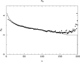
Figure 14: Momentum value, $p_{0}$, separating the people and king distribution as a function of time for the case with a total constant energy of $1,500,000$. The solid line is the theoretical value obtained with Eqs. (14) to (20) and Eqs. (31) and (33).

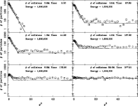
Figure 15: Same as Fig. 4 but with a total constant energy of $1,500,000$. The solid lines in this cases have been obtained with the experimental fit of $n_{p}$ (Fig. 11) and Eqs. (14) to (20) and Eqs. (31) and (33).

VIII Granular systems in presence of gravity seen as extremum complexity gases

Granular system in presence of gravity experiments consist of metal spheres allowed to move on a flat surface which is slightly tilted with respect to the horizontal plane and are thus subject to the force of gravity. The particles are forced to move by an oscillation bottom wall where they tend to fall once they dissipate enough energy by collisions. In these systems, it has been observed that the horizontal component velocity distribution of the particles is not Gaussian as would be expected in a system in equilibrium Kudrolli and Henry (2000) Rouyer and Menon (2000) Brey and Ruiz-Montero (2003). Although the theoretical details are not analyzed in this paper, the system is actually in a steady state mode and could be considered as being out of equilibrium. These experiments and simulations show diverse velocity distributions. Rouyer and Menon Rouyer and Menon (2000) show a distribution with an exponential behavior but an exponent different than two ($1.5$) as would correspond to a Gaussian distribution. Kudrolli and Henry Kudrolli and Henry (2000) show that the central portion of the velocity distribution is Gaussian for their experiments. Brey and Ruiz-Montero Brey and Ruiz-Montero (2003) numerical simulations show neither of them, but rather something in between depending on some properties of the system. In fact, some of these experiments are actually showing a double Gaussian or extremum complexity distribution function. This is the case in Fig. 2 of Kudrolli and Henry Kudrolli and Henry (2000), where a clear double Gaussian distribution function is shown. To make this more evident, we present in Fig. 16 the experimental points of Kudrolli and Henry (2000) and two fitted non-overlapping Gaussians.

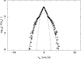
Figure 16: Non–overlapping Gaussian or extremum complexity distribution function (solid lines) which would match the experimental results of a granular system in the presence of gravity ( symbols as in Fig. 2 of Kudrolli and Henry Kudrolli and Henry (2000)).

IX Discussion

The extremum complexity approximation provides a simple, yet powerful way to simplify the dynamics of some systems out of equilibrium. This approximation relies on a property of the Frobenius–Perron operator which basically keeps regions of accessible phase space with zero probability if and only if the regions they originate from have also zero probability. This is the same as saying that systems out of equilibrium tend to prefer piecewise uniform distributions in the accessible phase space. The final consequence is that one particle distribution functions will behave as piecewise exponential functions for some systems, which makes the approximation relatively easy to apply to any system. We are only left with the task of delimiting the phase space regions for each one of the exponential distributions, the people and the king one. In this paper we have shown how a monodimensional gas consisting of $10,000$ particles can be described by just nine parameters providing a significant simplification.

One caveat of the extremum complexity approximation is that it seems to work for some particular systems. Then, one of the consequences of this is that it is not completely clear to which systems this method can be applied. Another drawback is that it is not always clear how to separate the different piecewise uniform distribution functions. In any case, the ultimate justification of approximations in statistical mechanics has always been that the results are useful in the real world. This can certainly be applied to the example shown here, the monodimensional ideal gas is enormously simplified and accurately described by using the extremum complexity approximation. Also some laboratory experiments with granular systems out of equilibrium, as that shown in Fig. 16, display a double Gaussian distribution.

Appendix A Derivation of the non-equilibrium distributions

Strictly speaking, the derivation of both non–equilibrium one–particle distributions (people and king) should be done using the accessible states of the system, which constitutes a surface in the N–dimensional phase space for an isolated system. In practice, it is far easier to make this calculation using the volume instead of the surface of the body that delimits the accessible states. We can readily switch from volumes to surfaces using the well known property that the volume of a sphere is proportional to its surface.

The proof will follow the technique shown in Lopez-Ruiz et al. (2007). If $x_{i}$ are the generalized coordinates or momentums of the Hamiltonian for particle $i$, $b$ is a parameter that defines the energy expression for the particle and the Hamiltonian for non-interacting particles is

$$H=x_{1}^{b}+x_{2}^{b}+\dots+x_{N}^{b},$$ (34)

then the accessible states of the system are defined by,

$$H\leq E,$$ (35)

where $E$ is the total energy the system can achieve. We will define the phase space volume inside the $E$ hypersurface by

$$V_{N}(\rho),$$ (36)

being $\rho$ the maximum value the generalized coordinate $x$ can achieve.

To this we need to add the limitations in phase space due to the non-equilibrium condition, piecewise uniform distribution or extremum complexity,

$$x_{min}\leq x_{i}\leq x_{MAX}.$$ (37)

The relationship between the N–dimensional volume in phase space and the volume in (N-1)-dimensional space is,

$$V_{N}(E^{\frac{1}{b}})=\int_{x_{min}}^{x_{MAX}}V_{N-1}((E-x^{b})^{\frac{1}{b}})dx.$$ (38)

The one particle distribution function, $f(x)$, will be proportional to the accessible states of the system,

$$f(x)=CV_{N-1}((E-x^{b})^{\frac{1}{b}}),$$ (39)

where $C$ is a constant. Taking into account that $f(x)$ should be normalized,

$$\int_{x_{min}}^{x_{MAX}}f(x)dx=1,$$ (40)

and combining Eq. (39) and Eq. (40) we get the following expression for $f(x)$,

$$f(x)=\frac{V_{N-1}((E-x^{b})^{\frac{1}{b}})}{V_{N}(E^{\frac{1}{b}})}.$$ (41)

Since the volume of an N-dimensional body as the one considered here is given by,

$$V_{N}(\rho)=g(N)\rho^{N},$$ (42)

we can substitute this in Eq. (41) and arranging terms we finally get,

$$f(x)=\frac{g(N-1)}{g(N)}\left(1-\frac{x^{b}}{E}\right)^{\frac{N-1}{b}}.$$ (43)

We know that the total maximum energy of the system, $E$, is proportional to the number of particles, $N$,

$$E=N\epsilon.$$ (44)

Note that because of the inequality of Eq. (37), $\epsilon$ will not be the mean energy per particle of the system. Introducing this last expression in Eq. (43) we obtain,

$$f(x)=\frac{g(N-1)}{g(N)}\left(1-\frac{x^{b}}{N\epsilon}\right)^{\frac{N-1}{b}},$$ (45)

and finally taking the limit for $N\rightarrow\infty$ we obtain the final expression,

$$f(x)=\quad\begin{cases}K{\rm e}^{-\frac{x^{b}}{\epsilon b}}&,\;x_{min}\leq x\leq x_{MAX}\\ 0&,\;x\leq x_{min}\;{\rm or}\;x\geq x_{MAX}\end{cases}$$ (46)

References

- Jaynes (1957) J. T. Jaynes, Phys. Rev. E 106, 620 (1957).
- Calbet and Lopez-Ruiz (2007) X. Calbet and R. Lopez-Ruiz, Physica A 382, 523 (2007).
- Kudrolli and Henry (2000) A. Kudrolli and J. Henry, Phys. Rev. E 62, R1489 (2000).
- Calbet and Lopez-Ruiz (2001) X. Calbet and R. Lopez-Ruiz, Phys. Rev. E 63, 066116(9) (2001).
- Lopez-Ruiz et al. (1995) R. Lopez-Ruiz, H. Mancini, and X. Calbet, Physics Letters A 209, 321 (1995).
- Martin et al. (2006) M. Martin, A. Plastino, and O. Rosso, Physica A 369, 439 (2006).
- Mackey (1992) M. C. Mackey, Springer-Verlag, Berlin pp. 24–25,40–41 (1992).
- Rouyer and Menon (2000) F. Rouyer and N. Menon, Phys. Rev. Lett. 85, 3676 (2000).
- Brey and Ruiz-Montero (2003) J. J. Brey and M. J. Ruiz-Montero, Phys. Rev. E 67, 021307 (2003).
- Lopez-Ruiz et al. (2007) R. Lopez-Ruiz, J. Sanudo, and X. Calbet, arXiv:0708.3761v2 [nlin.CD] (2007).