HRI-P-08-11-004

Hybrid textures in minimal seesaw mass matrices

Srubabati Goswami^1,2,  Subrata Khan¹,  Atsushi Watanabe^2
1Physical Research Laboratory, Navrangpura, Ahmedabad -380009, India,

²Harish-Chandra Research Institute, Chhatnag Road, Jhunsi, Allahabad -211019, India

In the context of minimal seesaw framework, we study the implications of Dirac and Majorana mass matrices in which two rigid properties coexist, namely, equalities among mass matrix elements and texture zeros. In the first part of the study, we discuss general possibilities of the Dirac and Majorana mass matrices for neutrinos with such hybrid structures. We then classify the mass matrices into realistic textures which are compatible with global neutrino oscillation data and unrealistic ones which do not comply with the data. Among the large number of general possibilities, we find that only 6 patterns are consistent with the observations at the level of the most minimal number of free parameters. These solutions have only 2 adjustable parameters, so that all the mixing angles can be described in terms of the two mass differences or pure numbers. We analyze these textures in detail and discuss their impacts for future neutrino experiments and for leptogenesis.

1 Introduction

The origin of the generation structure realized in nature is an engrossing subject which has been discussed for a long time, but still remains veiled. Within the standard electroweak theory, masses and mixing angles of fermions originate from the Yukawa interactions with the Higgs boson, responsible for the electroweak symmetry breaking. While, the relative strength of the gauge interactions for various fermion species are controlled by gauge invariance, Yukawa couplings are not governed by any principle. They bring a multitude of free parameters into the theory and even have ambiguities in reconstructing their values from experiments. A viable approach is, therefore, to search for mass matrices which are taking suggestive forms in light of model building ingredients, such as symmetry amongst generations.

A direct scheme in this spirit is “texture zero” in the mass matrices of fermions. In this framework, it is assumed that the mass matrices have several elements which are anomalously small compared to the others. Initially this approach was studied in the quark sector [1] and it was found that the existing relations among masses and mixings of quarks can be explained by the vanishing matrix elements. The available textures presented in the literature provide foundations of model building and insights into the generation puzzle.

As for the lepton sector, recent progress in neutrino physics makes it possible to discuss feasible forms for mass matrices. In [2] and many subsequent papers, the texture zeros in lepton sector have been discussed in the context of various types of mass matrices such as the Majorana mass matrix of the left-handed neutrinos [3], both the charged lepton and neutrino mass matrices [4], the Dirac and the Majorana mass matrices in the seesaw mechanism [5] and amalgamated Yukawa couplings in grand unification [6]. All these results also provide useful information to infer the structure lying behind the Yukawa interactions.

It is to be noted, that, for the mass matrices in the lepton sector, the situation is different from that of the quark sector because of the weak hierarchy of neutrino mass spectrum (for normal hierarchy) and two large mixing angles. In addition, the neutrino spectrum can also have inverted hierarchy and can even be quasi-degenerate which has no analogue in the quark sector. One of the most distinct features amongst observations in the neutrino sector is the small 1-3 angle against possible maximal 2-3 mixing. This is the origin of the $\mu$-$\tau$ symmetric nature of the neutrino mass matrix [7]. In the generation basis where the charged-lepton mass matrix is diagonal, the exact $\mu$-$\tau$ symmetric limit means that there are simple equalities among the matrix elements of the neutrino mass matrix. Moreover, the $\mu$-$\tau$ symmetric neutrino mass matrix contains the tri-bimaximal mixing [8] as a special case, which is obtained by requiring further special relations among the matrix elements. Thus, the equality between the matrix elements might play an important role in understanding the properties of neutrinos and become a simple and direct approach to search for “suggestive forms” of the mass textures.

The equalities among left-handed Majorana mass matrix elements were discussed in [9] in a bottom-up way. In [10], hybrid structures, with the coexistence of equalities among matrix elements and texture zeros for the left-handed Majorana mass matrix were studied. In this paper we follow the approach of [10], but consider the equalities and zeros in the Dirac and right-handed Majorana mass matrices in the seesaw mechanism. We perform a thorough classification of such hybrid textures and identify the left-handed Majorana mass matrices that can be reconciled with the inputs obtained from neutrino oscillation data. In particular, we consider the case where only two right-handed neutrinos take part in the seesaw mechanism [11]. Texture analysis in the context of such a minimal seesaw scheme has been accomplished in [12, 13]. An advantage of this choice is that there are less number of free parameters. Thus the mass matrices get simple forms and rich predictions compared to the standard three heavy neutrino models. By exhausting all possibilities, we find a novel class of textures which have only two adjustable parameters to fit the low-energy data. We discuss the possibility of having leptogenesis in these textures and explore the connection between high and low energy CP violation if any.

The layout of the paper goes as follows. In Section 2, we present the formulations which are needed for the subsequent discussions. In Section 3, we study equalities amongst mass matrix elements and enumerate general possible forms of the mass matrices with equality relations. In Section 4, we perform a combined analysis of equalities and texture zeros and discuss the viable minimal textures which are compatible with the current neutrino data. In Section 5, we discuss CP violation, paying particular attention to possible connections between leptogenesis and CP violation in neutrino oscillation. In Section 6, we briefly comment on the renormalization group effects for the mass matrices. Section 7 is devoted to conclusion and summary.

2 Formulation and the oscillation parameters

We assume that the tiny neutrino masses are generated through type-I seesaw mechanism [14, 15] by the suppression effect of the large mass scale of the right-handed neutrinos. By integrating out the heavy right-handed neutrinos, the Majorana mass matrix of the left-handed neutrinos is obtained as,

$$\mathcal{M}=-m_{D}^{\rm T}M_{R}^{-1}m_{D},$$ (2.1)

where $m_{D}$ denotes the Dirac mass matrix after the electroweak symmetry breaking, and $M_{R}$ is the Majorana mass matrix for the right-handed neutrinos. In this paper, we consider the case where we have only two right-handed neutrinos. Accordingly, the Dirac mass matrix $m_{D}$ is a $2\times 3$ rectangular matrix, while $M_{R}$ is given by a $2\times 2$ symmetric matrix. It is noteworthy that the two generations of fermions are matched well with the idea of the doublet (irreducible representation ) of discrete groups, which have recently been utilized to address the observed lepton mixings and masses.

The mixing matrix in the lepton sector, the so-called Pontecorvo-Maki-Nakagawa-Sakata (PMNS) matrix $V$ can be defined as the unitary matrix which diagonalizes the left-handed Majorana mass matrix $\mathcal{M}$ in the generation basis where the charged-lepton mass matrix is diagonal:

$$\mathcal{M}=V^{*}DV^{\dagger},$$ (2.2)

where $D\equiv{\rm diag}(m_{1},m_{2},m_{3})$. The neutrino oscillation experiments are capable of determining the squared mass differences $\Delta m^{2}_{ij}\equiv m_{i}^{2}-m^{2}_{j}$ and the three mixing angles and one CP violating phase in $V$. We parameterize the PMNS matrix $V$ as

$$V=P\begin{pmatrix}c_{12}c_{13}&s_{12}c_{13}&s_{13}e^{-i\delta}\\ -s_{12}c_{23}-c_{12}s_{23}s_{13}e^{i\delta}&c_{12}c_{23}-s_{12}s_{23}s_{13}e^{i\delta}&s_{23}c_{13}\\ s_{12}s_{23}-c_{12}c_{23}s_{13}e^{i\delta}&-c_{12}s_{23}-s_{12}c_{23}s_{13}e^{i\delta}&c_{23}c_{13}\\ \end{pmatrix}\begin{pmatrix}1&&\\ &e^{-i\rho}&\\ &&e^{-i\sigma}\\ \end{pmatrix},$$ (2.3)

where $c_{ij}$ and $s_{ij}$ stand for $\cos\theta_{ij}$ and $\sin\theta_{ij}$. The phase $\delta$ represents one phase degree of freedom which is responsible for CP violation phenomena at low-energy, while $\rho$ and $\sigma$ are the Majorana phases. $P$ is a diagonal phase matrix which is to be removed by the redefinition of the left-handed fields. So far, oscillation experiments have determined the two mass squared differences and the two angles, and have provided an upper bound on the third mixing angle $\theta_{13}$. The three generation analysis of the current data suggests

	best fit	$3\sigma$ range
$\Delta m_{21}^{2}$ [$10^{-5}{\rm eV}^{2}$]	7.6	7.1 - 8.3
$|\Delta m_{31}^{2}|$ [$10^{-3}{\rm eV}^{2}$]	2.4	2.0 - 2.8
$\sin^{2}\theta_{12}$	0.32	0.26 - 0.40
$\sin^{2}\theta_{23}$	0.50	0.34 - 0.67
$\sin^{2}\theta_{13}$	0.007	$\leq$ 0.05

Table 1: The present best-fit values and the 3$\sigma$ ranges of oscillation parameters from [16].

the $3\sigma$ ranges of the five oscillation parameters as presented in Table 1 [16]. Note that at present there is no constraint on any of the CP phases.

We note that, while for $\theta_{13}=0$ and $\theta_{23}=\pi/4$, $\mu$-$\tau$ symmetric nature is observed in the lepton mixing matrix, the charged-fermion masses do not respect this symmetry at all. If we regard the observed symmetric nature as a remnant of some exact symmetry at some high-energy scale, the symmetry should be broken strongly in the charged-fermion sector, whereas it must be broken weakly (or preserved) in the neutrino sector. A nontrivial task is, therefore, to realize such asymmetric breaking naturally [17]. We put aside this issue in the present work and just assume that probable equalities among matrix elements hold only in the neutrino sector, taking the charged-lepton mass matrix as diagonal. However, for the right-handed Majorana mass matrix we assume a most general form and do not consider it to be diagonal a priori.

It should be emphasized that, in the following analysis, the flavor basis of the left-handed neutrino (the $SU(2)$ lepton doublet) is always fixed, in such a way, that the permutations of the columns of the Dirac mass matrix $m_{D}$ change physical consequences. In general, there are 6 textures of $m_{D}$ which are associated with each other by permutation of the columns. We must take into account these 6 patterns as general possibilities, regarding them as independent textures which lead to different predictions.

3 The equalities among matrix elements

Before going to the study of coexistence of the equalities and vanishing elements in the mass matrices, we outline the handling of the equalities among mass matrix elements and discuss the situation where only equalities are imposed on the neutrino mass matrices.

In both Dirac and Majorana mass matrices, the matrix elements are in general complex valued. We impose the equalities among the matrix elements such that these are applicable not only to the absolute values of the matrix elements but also to the complex phases. We will comment on the un-removable phases of the matrix elements and CP violation of certain textures in Section 4, where we study the hybrid textures.

We start with the classification of the general possibilities of the Dirac mass matrix. It should be noted that, here and in what follows, the textures of $m_{D}$ are specified by the positions of the matrix elements which are connected with the other elements by equalities. At the stage of enumerating general possibilities, the locations of the vanishing elements specify the “identity” of the textures. For example, the equation $(m_{D})_{11}=(m_{D})_{12}$ symbolizes the texture

$$m_{D}=\begin{pmatrix}a&a&b\\ c&d&e\\ \end{pmatrix}.$$ (3.1)

Since there are 6 matrix elements in the Dirac mass matrix $m_{D}$, we can impose equality relations between matrix elements up to 5. We show the complete list of the possible equalities of $m_{D}$ in Appendix A.

Next let us discuss the Majorana mass matrix $M_{R}$. In this work, we take $M_{R}$ as a $2\times 2$ complex symmetric matrix, which means that there are 3 independent matrix elements in $M_{R}$. Therefore $M_{R}$ can accommodate at most 2 equalities. However, 2 equalities in $M_{R}$ imply a vanishing determinant. With such an $M_{R}$, there appears a state which does not receive seesaw suppression in mass. In this work, we do not consider such spectrum and in what follows we will simply exclude the cases where $M_{R}$ has two equalities. The three alternatives for $M_{R}$ (or $M_{R}^{-1}$) with 1 equality are:

$$M_{R}^{-1}=\begin{pmatrix}A&B\\ B&A\\ \end{pmatrix},\quad\begin{pmatrix}A&A\\ A&B\\ \end{pmatrix},\quad\begin{pmatrix}A&B\\ B&B\\ \end{pmatrix}.$$ (3.2)

Note that in $2\times 2$ case, the equalities in $M_{R}$ are directly connected to the equalities in $M_{R}^{-1}$. We will examine these three textures as general possibilities in the following discussions. We note that for the three textures in (3.2), all the matrix elements cannot be made real by re-definition of the right-handed neutrino fields. Thus, although 1 equality relation reduces the number of the free parameters by one, it does not reduce the number of the phases which can be rotated away from the Lagrangian. This is different from the case of texture zeros. If we impose 1 zero texture in $M_{R}$, there is no un-removable phase in the matrix.

Now we are in the stage to study the combination of $m_{D}$ and $M_{R}$ according to the total number of equalities to be distributed in them. First of all, it is easy to see that the case of total 7 or 6 equalities cannot be viable because they would either need 5 equalities in $m_{D}$ or 2 equalities in $M_{R}$ or both together.

The next possibility is total 5 equalities. In this case, there is only one option that satisfy our selection criteria namely,

• 4 equalities in $m_{D}$ and 1 equality in $M_{R}$

For this case, from the 7 representatives of $m_{D}$ in Appendix A.4 and 3 patterns of (3.2), we have

$$m_{D} = \begin{pmatrix}a&a&a\\ a&a&b\\ \end{pmatrix},\begin{pmatrix}a&a&a\\ a&b&b\\ \end{pmatrix},\begin{pmatrix}a&a&b\\ a&b&a\\ \end{pmatrix},\begin{pmatrix}a&a&b\\ a&b&b\\ \end{pmatrix},\begin{pmatrix}a&a&b\\ b&b&a\\ \end{pmatrix},$$

$$M_{R}^{-1} = \begin{pmatrix}A&B\\ B&A\\ \end{pmatrix},\begin{pmatrix}A&A\\ A&B\\ \end{pmatrix},\begin{pmatrix}A&B\\ B&B\\ \end{pmatrix}.$$ (3.3)

Note that in (3.3), we have dropped the two Dirac mass matrices containing rows that are not independent of each other. With these forms of $m_{D}$, we obtain $\mathcal{M}$ which has only one massive state because we can rotate the right-handed fields in such a way that only one right-handed neutrino is coupled with the left-handed neutrinos. We can therefore exclude these two cases from the viable possibilities.

Note also that in (3.3), the Dirac mass matrices presented are the ”representatives” from which all possible forms of $m_{D}$ are generated. Thus (3.3) actually contains large number of the combinations. For instance, corresponding to the first $m_{D}$ in (3.3), there are 5 other associated forms. Accordingly, we must understand that there are $6\times 3$ combinations of $m_{D}$ and $M_{R}$ for the first $m_{D}$ presented in (3.3). However, not all of these combinations are independent. They contain the combinations which are associated with each other by the permutation of the two right-handed neutrinos. Thus, it is sufficient to take account of the column exchanges of each $m_{D}$ in (3.3).

Finally, we comment on the case of total 4 equalities. There are two possible options to be considered, for distributing 4 equalities in $m_{D}$ and $M_{R}$.

• 4 equalities in $m_{D}$ and 0 equality in $M_{R}$

• 3 equalities in $m_{D}$ and 1 equality in $M_{R}$

These two cases cannot be excluded a priori and we regard them as general possibilities for total 4 equalities:

$$m_{D} = \begin{pmatrix}a&a&a\\ a&a&b\\ \end{pmatrix},\begin{pmatrix}a&a&a\\ a&b&b\\ \end{pmatrix},\begin{pmatrix}a&a&b\\ a&a&b\\ \end{pmatrix},\begin{pmatrix}a&a&b\\ a&b&a\\ \end{pmatrix},$$

$$\begin{pmatrix}a&a&a\\ b&b&b\\ \end{pmatrix},\begin{pmatrix}a&a&b\\ a&b&b\\ \end{pmatrix},\begin{pmatrix}a&a&b\\ b&b&a\\ \end{pmatrix},$$

$$M_{R}^{-1} = \begin{pmatrix}A&B\\ B&C\\ \end{pmatrix},$$ (3.4)

and

$$m_{D} = \begin{pmatrix}a&a&a\\ b&b&c\\ \end{pmatrix},\begin{pmatrix}a&a&b\\ a&b&c\\ \end{pmatrix},\begin{pmatrix}a&a&b\\ a&c&b\\ \end{pmatrix},\begin{pmatrix}a&a&c\\ a&b&b\\ \end{pmatrix},\begin{pmatrix}a&a&b\\ b&c&a\\ \end{pmatrix},\begin{pmatrix}a&a&c\\ b&b&a\\ \end{pmatrix},$$

$$\begin{pmatrix}a&a&a\\ a&b&c\\ \end{pmatrix},\begin{pmatrix}a&a&b\\ a&a&c\\ \end{pmatrix},\begin{pmatrix}a&a&b\\ a&c&a\\ \end{pmatrix},\begin{pmatrix}a&b&c\\ a&b&c\\ \end{pmatrix},\begin{pmatrix}a&a&c\\ b&b&c\\ \end{pmatrix},\begin{pmatrix}a&b&c\\ b&a&c\\ \end{pmatrix},$$

$$\begin{pmatrix}a&a&c\\ c&b&b\\ \end{pmatrix},\begin{pmatrix}a&b&c\\ c&a&b\\ \end{pmatrix},$$

$$M_{R}^{-1} = \begin{pmatrix}A&B\\ B&A\\ \end{pmatrix},\begin{pmatrix}A&A\\ A&B\\ \end{pmatrix},\begin{pmatrix}A&B\\ B&B\\ \end{pmatrix}.$$ (3.5)

We note that there are at most 2 un-removable phases in the above textures (3.4) and (3.5). However, with a vanishing matrix element, the number of the un-removable phases is reduced to one.

4 Hybrid texture analysis

In this section, we show the results of the combined analysis of the equalities and the texture zeros, according to the total number of the reductions of the free parameters. One of our aim is to make a list of the realistic forms of $m_{D}$ and $M_{R}$ which have as small number of independent parameters as possible. In other words, we search for the textures which have the strongest predictive power with the coexistence of the vanishing elements and the equalities among matrix elements.

Before going to the discussions, we should define the procedure to impose the equalities and texture zeros on the mass matrices that we have followed. We impose texture zeros on the mass matrices after introducing the equalities among the matrix elements. For instance if we consider the $m_{D}$ of (A.36) and put $b=0$ then we get

$$\begin{pmatrix}a&a&b\\ b&b&a\\ \end{pmatrix}\,\to\,\begin{pmatrix}a&a&0\\ 0&0&a\\ \end{pmatrix},$$ (4.1)

the resultant texture belong to 4 equality and 1 zero. Note that we do not impose texture zeros on each entry, but rather force the parameter $b$ to be zero. On the other hand, if we consider (A.21) and put $b=0$ and $c=0$ we get,

$$\begin{pmatrix}a&a&c\\ b&b&a\\ \end{pmatrix}\,\to\,\begin{pmatrix}a&a&0\\ 0&0&a\\ \end{pmatrix}.$$ (4.2)

Thus, after putting the zeros, the resultant matrix is the same in both cases though (4.2) is obtained by setting two different parameters to be zero. In that sense (4.2) belongs to 3 equalities and 2 zeros denoting the fact that the zeros have originated from different parameters. Such a classification is justified because strictly speaking, when we impose texture zeros then it does not imply exact zero element but some matrix element which is anomalously small compared to the other elements. Therefore in the most general scenario the two matrices can belong to different categories although the total number of reductions remain the same. However, it is to be noted that in our present work we have treated a zero as an exact zero and from this viewpoint both (4.1) and (4.2) will give identical results for the predictions of masses and mixing angles. Therefore once we consider the case of 4 equalities and 1 zero we need not redo the calculations for 3 equalities and 2 zeros. Generalizing the above we can say that in our calculations when we put more than one zero in any of the matrices, it eventually increases the number of equalities of that matrix and reduce the number of zeros. Thus $m$ equalities and $n$ zeros already gets considered under $m+1$ equalities and $n-1$ zeros. One can continue this reduction till $n=2$. Thus maximum number of zeros in any reduction is 2, distributed as one zero in $m_{D}$ and one zero in $M_{R}$.

The maximum possible number of reductions that one can get in minimal seesaw model is 7. The parameter reductions can be distributed as equalities and zeros according to the following tables (for total 7 and 6 reduction cases):

Total 7 reductions		Total 6 reductions
equality zero results 7 0 $\times$ 6 1 $\times$ 5 2 $\times$ 4 3 $\times$ 3 4 $\times$ $\vdots$ $\vdots$ $\times$		equality zero results 6 0 $\times$ 5 1 $\bigcirc$ 4 2 $\bigcirc$ 3 3 $\times$ 2 4 $\times$ $\vdots$ $\vdots$ $\times$

In the tables, the symbol “$\bigcirc$” means there are textures which are compatible to the current oscillation data, and the symbol “$\times$” means there is no such viable one in each case. The general textures in each case are created, for example, by imposing the zero elements on (3.3), (3.4) and (3.5). By thorough examinations of all possibilities, we find three viable textures in 5 equalities + 1 zero and 4 equalities + 2 zero cases, and three almost viable textures in 4 equalities + 2 zero case. On the other hand, no viable solution exists at the level of 7 reductions.

In the 7 reductions, all possible textures amount to $\mathcal{M}$ with integer entries up to overall factor made out of the scales in $m_{D}$ and $M_{R}$. An interesting feature of this type of matrices is that they can provide hierarchy among their eigenvalues by cancellation of the numerical factors. Since it is unlikely for the usual groups that the Clebsch-Gordan coefficients present strong hierarchies among themselves, the realization of the mass hierarchy along the above line gives an insight into model building for the charged fermion sectors with flavor symmetry [18].

We note that, except for some particular cases, there are CP violating phases in each texture at the level of 6 reductions. Although these phases can affect physics, we have neglected them in the texture analysis, regarding all the parameters in the mass matrices as real valued. Namely, we pick up those mass textures which can be compatible with the data without the help of the phases. This simplification may exclude the possibility of the textures which can be made viable only with nontrivial values of the phases. A complete survey of this kind of textures needs more laborious calculations which is beyond the scope of this paper.

Table 2 shows the three viable and the three “quasi viable” textures. Besides the 6 patterns in the table, there exist other 6 textures which can be obtained by permuting 2-3 column of $m_{D}$. Although such 6 counterparts are independent solutions, we present only 6 textures because those predictions are almost the same as the solutions in Table 2. Note also that we can create other viable solutions by relaxing the equalities of the solutions presented in the table. Such daughter textures have less predictions than the original solutions according to the number of the equalities that are relaxed. However, such solutions may also be of interest because it is practically easier to realize moderate textures rather than the solutions in Table 2 themselves in the context of usual model building.

In the following, we discuss the viable textures, focusing on salient features of these solutions and the implications for future experiments and leptogenesis.

	$m_{D}$,      $M_{R}^{-1}$	NH	IH	$\sin^{2}\theta_{12}$	$\sin^{2}\theta_{13}$	$\sin^{2}\theta_{23}$	$|m_{ee}|$
I	$\begin{pmatrix}a&a&a\\ 0&a&a\\ \end{pmatrix}$, $\begin{pmatrix}A&A\\ A&B\\ \end{pmatrix}$	$\times$	$\bigcirc$	$\simeq\frac{1}{{3}}$	0	$\frac{1}{{2}}$	$\simeq\frac{1}{3}\sqrt{\Delta m^{2}_{31}}$
II	$\begin{pmatrix}b&a&a\\ a&b&b\\ \end{pmatrix}$, $\begin{pmatrix}A&A\\ A&0\\ \end{pmatrix}$	$\times$	$\bigcirc$	$\simeq{\frac{3-\sqrt{2}}{6}}$	0	$\frac{1}{{2}}$	$\simeq\frac{\sqrt{2}}{3}{\Delta m^{2}_{31}}$
III	$\begin{pmatrix}b&a&a\\ a&b&0\\ \end{pmatrix}$, $\begin{pmatrix}0&B\\ B&B\\ \end{pmatrix}$	$\times$	$\bigcirc$	$\simeq 0.31$	$\simeq 0.04$	$\simeq 0.52$	$\simeq 0.527\sqrt{\Delta m^{2}_{31}}$
IV	$\begin{pmatrix}a&b&a\\ 0&a&b\\ \end{pmatrix}$, $\begin{pmatrix}A&0\\ 0&A\\ \end{pmatrix}$	$\bigcirc$	$\times$	0.23	0.05	0.49	0.0043 eV
V	$\begin{pmatrix}a&a&b\\ 0&b&a\\ \end{pmatrix}$, $\begin{pmatrix}0&B\\ B&0\\ \end{pmatrix}$	$\bigcirc$	$\times$	0.24	0.04	0.49	0
VI	$\begin{pmatrix}0&c&b\\ c&b&0\\ \end{pmatrix}$, $\begin{pmatrix}A&A\\ A&0\\ \end{pmatrix}$	$\bigcirc$	$\times$	0.19	0.04	0.50	0

Table 2: The three minimal solutions (I, II, III) and the three “quasi viable” solution (IV, V, VI). The column “NH” and “IH” means the normal and the inverted hierarchy respectively. The symbol “$\bigcirc$” means each texture can accommodate each mass ordering, and “$\times$” means it cannot. For I, II and III, the three mixing angles and the averaged mass parameter for the neutrino-less double beta decay are given to the $0^{th}$ order approximation in powers of $\alpha=\Delta m^{2}_{21}/|\Delta m^{2}_{31}|$. The decimals in the solutions III represent irrational factors which have too long expressions to be shown, whereas the decimals in the solution IV, V and VI are the predictions with the current best fit value of $\alpha$. The detailed discussions for I and II are given below (4.3) and (4.13) and for III is found below (4.20).

4.1 The solution I

Let us first discuss the solution I;

$$m_{D}=\begin{pmatrix}a&a&a\\ 0&a&a\\ \end{pmatrix},\quad M_{R}^{-1}=\begin{pmatrix}A&A\\ A&B\\ \end{pmatrix}.$$ (4.3)

After the seesaw mechanism, the Majorana mass matrix for the left-handed neutrinos becomes

$$\mathcal{M}\,=\,\begin{pmatrix}A^{\prime}&2A^{\prime}&2A^{\prime}\\ 2A^{\prime}&3A^{\prime}+B^{\prime}&3A^{\prime}+B^{\prime}\\ 2A^{\prime}&3A^{\prime}+B^{\prime}&3A^{\prime}+B^{\prime}\\ \end{pmatrix},$$ (4.4)

where we introduce the parameter $A^{\prime}\equiv a^{2}A$ and $B^{\prime}\equiv a^{2}B$ to simplify the notation. Note that this matrix obeys the so called scaling property between the second and third rows and second and third columns [19]. This matrix has $\mu$-$\tau$ symmetry and a zero eigenvalue such that the mass ordering is predicted to be inverted. Moreover, the reactor and the atmospheric angles are given as $\theta_{13}=0$ and $\theta_{23}=45^{\circ}$. A nontrivial consequence of this solution is thus the relation between masses and the solar angle. The two nonzero eigenvalues are

$$\lambda_{\pm}=\frac{1}{2}\left(7A^{\prime}+2B^{\prime}\pm\sqrt{57A^{\prime 2}+20A^{\prime}B^{\prime}+4B^{\prime 2}}\right).$$ (4.5)

We find that these eigenvalues should be identified as $\lambda_{+}=\sqrt{|\Delta m^{2}_{31}|+\Delta m^{2}_{21}}$ and $\lambda_{-}=-\sqrt{|\Delta m^{2}_{31}|}$ in order to fit the observations. The parameters $A^{\prime}$ and $B^{\prime}$ are therefore fixed in terms of the two mass differences as

$$A^{\prime} \simeq -\sqrt{|\Delta m^{2}_{31}|}\left(\frac{1}{3}+\frac{1}{18}\alpha+\mathcal{O}(\alpha^{2})\right),$$

$$B^{\prime} \simeq \sqrt{|\Delta m^{2}_{31}|}\left(\frac{7}{6}+\frac{4}{9}\alpha+\mathcal{O}(\alpha^{2})\right),$$ (4.6)

where $\alpha\equiv\Delta m^{2}_{21}/|\Delta m^{2}_{31}|$. Here we are taking a combination of the solutions which is viable with the solar neutrino observations. The solar angle is also fixed by the two mass differences. It is given by

$$\sin\theta_{12}\,=\,\frac{1+x}{\sqrt{8x^{2}+(1+x)^{2}}},$$ (4.7)

where

$$x\equiv\frac{1}{18}\left(\sqrt{1+\alpha}-1-\sqrt{2+34\sqrt{1+\alpha}+\alpha}\right),$$ (4.8)

By expanding (4.7) in powers of $\alpha$, we find

$$\sin\theta_{12}\,\simeq\,\frac{1}{\sqrt{3}}\,-\,\frac{1}{6\sqrt{3}}\alpha\,+\,\mathcal{O}(\alpha^{2}).$$ (4.9)

It is interesting to observe that, in the 0-th order, the solar mixing angle is predicted to be $1/\sqrt{3}$, which is the same as in the tri-bimaximal mixing scenario. In fact, the whole mixing matrix $V$ can be written as

$$V\,\simeq\,\begin{pmatrix}-\frac{2}{\sqrt{6}}&\frac{1}{\sqrt{3}}&0\\ \frac{1}{\sqrt{6}}&\frac{1}{\sqrt{3}}&\frac{-1}{\sqrt{2}}\\ \frac{1}{\sqrt{6}}&\frac{1}{\sqrt{3}}&\frac{1}{\sqrt{2}}\\ \end{pmatrix}\begin{pmatrix}1&\frac{\alpha}{6\sqrt{2}}&0\\ -\frac{\alpha}{6\sqrt{2}}&1&0\\ 0&0&1\\ \end{pmatrix}$$ (4.10)

up to $\mathcal{O}(\alpha)$. Thus, this is given by the tri-bimaximal mixing matrix multiplied by the small correction matrix. This type of lepton mixing is naturally realized by a class of flavor models which utilize the Scherk-Schwarz twisted boundary conditions [20]. It might be interesting to study this type of deviation from the tri-bimaximal mixing and its implication for future neutrino experiments systematically.

The effective neutrino mass $|m_{ee}|$ which is responsible for the neutrino-less double beta decay is given by the element $A^{\prime}$ itself. Thus in this texture we find $|m_{ee}|$ is predicted as

$$|m_{ee}|\,\simeq\,\frac{1}{3}\sqrt{|\Delta m^{2}_{31}|}\,=\,0.016\quad{\rm eV}$$ (4.11)

at the best fit of the mass difference. With this value, neutrino-less double beta decay may be detectable in forthcoming experiments.

Since there are only two mixing angles in $V$, CP must be conserved at low energy. However, at high energy there is one unremovable phase which can violate CP. Such CP violation is conveniently measured by the weak basis invariant $I_{h}={\rm Im}{\rm Tr}\Big{[}hHM_{R}^{*}h^{*}M_{R}\Big{]}$ where $h\equiv m_{D}^{*}m_{D}^{\rm T}$ and $H\equiv M_{R}^{\dagger}M_{R}$ [21]. For the texture I, we find

$$I_{h}=\frac{a^{4}(A^{2}-4|A-B|^{2})B\sin\phi_{B}}{|A-B|^{4}A^{3}}$$ (4.12)

in the basis where only $B$ is complex; $B\to Be^{i\phi_{B}}$. The leptogenesis [22] is thus possible, with the lepton asymmetry proportional to this quantity.

4.2 The solution II

Next we discuss the solution II;

$$m_{D}=\begin{pmatrix}b&a&a\\ a&b&b\\ \end{pmatrix},\quad M_{R}^{-1}=\begin{pmatrix}A&A\\ A&0\\ \end{pmatrix}.$$ (4.13)

After the seesaw mechanism, the Majorana mass matrix for the left-handed neutrinos becomes

$$\mathcal{M}\,=\,\begin{pmatrix}b^{\prime}(2a^{\prime}+b^{\prime})&a^{\prime 2}+a^{\prime}b^{\prime}+b^{\prime 2}&a^{\prime 2}+a^{\prime}b^{\prime}+b^{\prime 2}\\ a^{\prime 2}+a^{\prime}b^{\prime}+b^{\prime 2}&a^{\prime}(a^{\prime}+2b^{\prime})&a^{\prime}(a^{\prime}+2b^{\prime})\\ a^{\prime 2}+a^{\prime}b^{\prime}+b^{\prime 2}&a^{\prime}(a^{\prime}+2b^{\prime})&a^{\prime}(a^{\prime}+2b^{\prime})\\ \end{pmatrix},$$ (4.14)

where we define $a^{\prime}\equiv a\sqrt{A}$ and $b^{\prime}\equiv b\sqrt{A}$ to simplify the notation. As in the previous case, this matrix also has $\mu$-$\tau$ symmetry and a zero eigenvalues. The mass hierarchy is thus predicted as inverted ordering, and the reactor and the atmospheric angles are given as $\theta_{13}=0$ and $\theta_{23}=45^{\circ}$. The two nonzero eigenvalues are

$$\lambda_{\pm}=\frac{1}{2}\left(2a^{\prime 2}+6a^{\prime}b^{\prime}+b^{\prime 2}\pm\sqrt{3}\sqrt{4a^{\prime 4}+8a^{\prime 3}b^{\prime}+8a^{\prime 2}b^{\prime 2}+4a^{\prime}b^{\prime 3}+3b^{\prime 4}}\right),$$ (4.15)

We find that these eigenvalues should be identified as $\lambda_{+}=\sqrt{|\Delta m^{2}_{31}|+\Delta m^{2}_{21}}$ and $\lambda_{-}=-\sqrt{|\Delta m^{2}_{31}|}$ in order to fit the observations. A solution of this equation system is found to be

$$a^{\prime}\,\simeq\,\left(|\Delta m^{2}_{31}|\right)^{1/4}\left(\frac{(3+\sqrt{7})\sqrt{-2+\sqrt{7}}}{3\cdot 2^{3/4}}\,+\,\frac{7\sqrt{14}+16\sqrt{7}+7\sqrt{2}-56}{336\cdot 2^{1/4}\sqrt{-2+\sqrt{7}}}\,\alpha\,+\,\mathcal{O}(\alpha^{2})\right),$$

$$b^{\prime}\,\simeq\,\left(|\Delta m^{2}_{31}|\right)^{1/4}\left(-\frac{2^{1/4}\sqrt{-2+\sqrt{7}}}{3}\,+\,\frac{-7\sqrt{14}+2\sqrt{7}+14\sqrt{2}+14}{168\cdot 2^{1/4}\sqrt{-2+\sqrt{7}}}\,\alpha\,+\,\mathcal{O}(\alpha^{2})\right).$$

(4.16)

Here we show approximate expressions for $a^{\prime}$ and $b^{\prime}$ because the exact expressions are too long and complicated to present here. The solar angle is also fixed by the two mass differences. It is written in terms of $a^{\prime}$ and $b^{\prime}$, and the mass differences as

$$\sin\theta_{12} \,=\, \left|\frac{-2a^{\prime}(a^{\prime}+2b^{\prime})+\lambda_{+}}{\sqrt{2(a^{\prime 2}+a^{\prime}b^{\prime}+b^{\prime 2})^{2}+(-2a^{\prime}(a^{\prime}+2b^{\prime})+\lambda_{+})^{2}}}\right|$$ (4.17)

$$\simeq \sqrt{\frac{3-\sqrt{2}}{6}}\,-\,\frac{3\sqrt{2}-2}{16\sqrt{3}(3-\sqrt{2})^{3/2}}\alpha\,+\,\mathcal{O}(\alpha^{2})$$

$$\,=\, 0.514-0.0405\,\alpha+0.0258\,\alpha^{2}\,+\,\mathcal{O}(\alpha^{3}).$$

We can see that the prediction for the solar angle agrees with the current $3\sigma$ range although it is close to its lower bound.

The averaged neutrino mass $|m_{ee}|$ which is responsible for the neutrino-less double beta decay is given by $b^{\prime}(2a^{\prime}+b^{\prime})$ in this case. We find $|m_{ee}|$ is predicted as

$$|m_{ee}|\,\simeq\,\frac{\sqrt{2}}{3}\sqrt{|\Delta m^{2}_{31}|}\,=\,0.023\quad{\rm eV}$$ (4.18)

at the best fit of the mass difference and a signal can be expected in future We have a slightly better chance to detect neutrino-less double beta decay measurements.

CP violation is possible at high-energy as the weak-basis invariant $I_{h}$ is non-vanishing. In fact, it becomes

$$I_{h}=\frac{2ab\left(a^{2}-b^{2}-3ab\cos\phi_{b}\right)\sin\phi_{b}}{A^{4}}$$ (4.19)

in the basis where only $b$ is complex; $b\to be^{i\phi_{b}}$. On the other hand, no CP violation occurs in the neutrino oscillation because of the vanishing $\theta_{13}$.

4.3 The solution III

Finally let us discuss the solution III. The viable texture is given by

$$m_{D}=\begin{pmatrix}b&a&a\\ a&b&0\\ \end{pmatrix},\quad M_{R}^{-1}=\begin{pmatrix}0&B\\ B&B\\ \end{pmatrix}.$$ (4.20)

After the seesaw mechanism, the Majorana mass matrix for the left-handed neutrinos becomes

$$\mathcal{M}\,=\,\begin{pmatrix}a^{\prime}(a^{\prime}+2b^{\prime})&a^{\prime 2}+a^{\prime}b^{\prime}+b^{\prime 2}&a^{\prime 2}\\ a^{\prime 2}+a^{\prime}b^{\prime}+b^{\prime 2}&b^{\prime}(2a^{\prime}+b^{\prime})&a^{\prime}b^{\prime}\\ a^{\prime 2}&a^{\prime}b^{\prime}&0\\ \end{pmatrix},$$ (4.21)

where we introduce the parameter $a^{\prime}\equiv a\sqrt{B}$ and $b^{\prime}\equiv b\sqrt{B}$ to simplify the notation. This has one zero element in the final matrix and has been discussed in [23]. Unlike the two solutions found in the previous subsection, there is no $\mu$-$\tau$ symmetry in (4.21). Therefore the reactor and the atmospheric angles no longer satisfy $\theta_{13}=0$ and $\theta_{23}=45^{\circ}$, and all nonzero values of the mixing angles can be described as functions of the mass differences. We note that, because of the lack of the $\mu$-$\tau$ symmetry, there appears an additional solution in this case. Namely, the $m_{D}$ which is obtained by 2-3 column exchange of (4.20) can also be compatible with the data. Although these two solutions are independent in the sense that they are not related to each other by basis rotations, their physical consequences are almost the same. We thus discuss only (4.20) to illustrate important features of these solutions.

The two nonzero eigenvalues of (4.21) are

$$\lambda_{\pm}=\frac{1}{2}\left(a^{\prime 2}+4a^{\prime}b^{\prime}+b^{\prime 2}\pm\sqrt{9a^{\prime 4}+8a^{\prime 3}b^{\prime}+14a^{\prime 2}b^{\prime 2}+8a^{\prime}b^{\prime 3}+5b^{\prime 4}}\right).$$ (4.22)

We find that these eigenvalues should be identified as $\lambda_{-}=-\sqrt{|\Delta m^{2}_{31}|+\Delta m^{2}_{21}}$ and $\lambda_{+}=\sqrt{|\Delta m^{2}_{31}|}$ in order to fit the observations. The parameters $a^{\prime}$ and $b^{\prime}$ are therefore fixed in terms of the two mass differences. However, the exact expressions are too long and complicated and it is not appropriate to present them here. Instead, we shall approximate them in powers of $\alpha$;

$$a^{\prime} \simeq -\left(|\Delta m^{2}_{31}\right|)^{1/4}\left(0.848+0.116\,\alpha+\mathcal{O}(\alpha^{2})\right),$$

$$b^{\prime} \simeq \left(|\Delta m^{2}_{31}\right|)^{1/4}\left(0.227+0.201\,\alpha+\mathcal{O}(\alpha^{2})\right).$$ (4.23)

Here we are picking up a combination of the solutions for $\lambda_{-}=-\sqrt{|\Delta m^{2}_{31}|+\Delta m^{2}_{21}}$ and $\lambda_{+}=\sqrt{|\Delta m^{2}_{31}|}$, which gives the correct mixing angles. Note that we represent the leading and the first order coefficients by decimal numbers. These terms can also be represented as functions of integers as in (4.16), but the expressions are not so simple as in the case of the other two solutions. The three angles are also fixed by the two mass differences. They are given by

$$\sin\theta_{12}\,\simeq\,0.561+0.00775\,\alpha+\mathcal{O}(\alpha^{2}),$$ (4.24)

$$\sin\theta_{23}\,\simeq\,0.719+0.0171\,\alpha+\mathcal{O}(\alpha^{2}),$$ (4.25)

$$\sin\theta_{13}\,\simeq\,0.193+0.149\,\alpha+\mathcal{O}(\alpha^{2}).$$ (4.26)

Here we note again that the decimals in the above expressions represent definite irrational numbers which are too long and complicated to be presented in closed form. It is interesting that the predictions for $\theta_{12}$ and $\theta_{23}$ are very close to the current best fit values indicated in Table 1. We see that this texture predicts a relatively large $\theta_{13}$ which can be measured in forthcoming experiments like Double-Chooz.

The effective neutrino mass $|m_{ee}|$ which is responsible for the neutrino-less double beta decay is given by $|m_{ee}|=|a^{\prime}(a^{\prime}+2b^{\prime})|$ and is predicted as

$$|m_{ee}|\,\simeq\,0.527\sqrt{|\Delta m^{2}_{31}|}\,=\,0.026\quad{\rm eV}$$ (4.27)

at the best fit of the mass difference. Thus, neutrino-less double beta decay will be detectable in forthcoming experiments.

Finally we comment on CP violation. Since $\theta_{13}$ is nonzero with the solution III, one might expect that there exists corelation between CP violation phenomena at high and low-energy scale. However, this is not the case. The invariant measure $I_{h}$ is given by $I_{h}={\rm Im}\Big{[}h_{12}^{2}-2h_{11}h_{12}^{*}-2h_{12}h_{22}\Big{]}/|B|^{4}$, but $h_{12}$ is real valued for the $m_{D}$ in (4.20). Thus the leptogenesis does not occur with the solution III. On the other hand, the phase $\delta$ in the PMNS matrix is not vanishing. The CP violation caused by $\delta$ can be conveniently described with, for example, $I_{l}={\rm Tr}\Big{[}\mathcal{M}\mathcal{M}^{\dagger},m_{l}m_{l}^{\dagger}\Big{]}^{3}$, where $m_{l}$ is the charged-lepton mass matrix [24]. It is easily seen that the basis-independent quantity $I_{l}$ takes the form $I_{l}=C_{1}\cdot{\rm Im}\Big{[}ab^{*}\Big{]}+C_{2}\cdot{\rm Im}\Big{[}a^{2}b^{*}{}^{2}\Big{]}$, where $C_{1}$ and $C_{2}$ are nonzero real values, and $I_{l}$ is therefore nonzero in general. To summarize, with the solution III, CP violation in the oscillation can be measured, while leptogenesis is not possible.

4.4 The solution IV, V and VI

Interestingly, the three solutions I, II and III are consistent only with the inverted mass ordering for neutrino mass spectrum. From this fact, we conclude that the hybrid property prefers the inverted hierarchy. However, there exist three quasi viable textures IV, V and VI with normal hierarchy. We call them quasi-viable as certain predictions of these textures are marginally consistent with the $3\sigma$ range presented in Table 1, This can be seen, for example, with V and VI in which the element $\mathcal{M}_{11}$ is vanishing. As a general consequence of $\mathcal{M}_{11}=0$ and the normal hierarchy with $m_{1}=0$, the solar and reactor angles correlate with $\alpha$ as $\tan\theta_{13}/\sin\theta_{12}=\alpha^{1/4}$. This relation needs small $\theta_{12}$ and $\alpha$, and large (just below the current $3\sigma$ bound) $\theta_{13}$.

With the solutions IV and V, there are is no CP violating phase for the right-handed mass matrix since the heavy neutrino are degenerate in mass. Such degeneracy can be relaxed by some corrections, for example, renormalization group evolution from the texture scale (at which the textures are assumed) down to the right-handed neutrino scale. However, even with relaxations of the degeneracy, the lepton asymmetries for IV and V are small because the off-diagonal components of $m_{D}^{*}m_{D}^{\rm T}$ are real valued. It may be possible to generate a non-zero value for this by introducing two-loop renormalization group effects [25]. In this paper we do not consider these effects.

On the other hand, we have nonzero $I_{h}$ and $I_{l}$ within the solution VI. Therefore the texture VI can give rise to a connection between leptogenesis and CP violation in neutrino oscillation. We discuss this connection in detail in the next section.

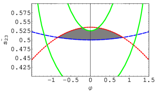
Figure 1: Constraints from the low-energy data (Table 1) on the $\varphi$-$\tilde{s}_{23}$ plane. The green (solid) curves shows the upper and lower bounds for the mass ratio $\alpha$. The blue (dashed) and red (dotted) curves correspond to the upper bound for $\theta_{13}$ and lower bound for $\theta_{12}$, respectively. The shaded region is allowed.

5 CP violation at high and low-energy scales

With the solution VI, both $I_{h}$ and $I_{l}$ are non-vanishing, and there is a correlation between CP violation phenomena at high and low-energy scales. It is interesting if we can predict the amount of CP violation at low energy in terms of the phase of the Yukawa coupling responsible for successful baryogenesis via leptogenesis. In this section, we address this issue and study the connection between leptogenesis and CP violation at low energy with the interesting example of the solution VI.

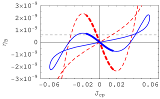
Figure 2: A parametric plot for the baryon-to-photon ratio $\eta_{B}(\varphi)$ and the Jarlskog invariant $J_{\rm CP}(\varphi)$, as functions of the phase parameter $\varphi$. The Horizontal dashed line is the constraint by the WMAP observation $\eta_{B}=6\times 10^{-10}$ [27]. The dashed curve is for the heavy neutrino scale $A=10^{-13.5}\,{\rm GeV^{-1}}$, and the solid curve is for $A=10^{-13}\,{\rm GeV^{-1}}$. For each curve, the thick line corresponds to the parameter range $-0.7<\varphi<0.7$ where the low-energy observables are consistent with the data, whereas the thin curve corresponds to the other region.

To perform this program, it is convenient to parameterize the Dirac mass matrix $m_{D}$ as [26]

$$m_{D}=\begin{pmatrix}0&0&xe^{i\varphi}\\ 0&y&ze^{i\varphi^{\prime}}\\ \end{pmatrix}\widetilde{V}^{T}\cdot\widetilde{P},$$ (5.1)

where $x,y,z$ are positive-real parameters, and $\widetilde{V}$ is an unitary matrix which contains only one Dirac type phase (conveniently parameterized as (2.3) without Majorana phases), and $\widetilde{P}$ is a diagonal phase matrix. Taking account of the texture zeros and equalities in $m_{D}$ of the solution VI, the general form (5.1) is reduced to

$$m_{D}=Z^{\rm T}\cdot\widetilde{V}^{T}\cdot\widetilde{P},$$ (5.2)

where $\widetilde{P}={\rm diag}(e^{i2\varphi},e^{i\varphi},1)$ and

$$Z^{\rm T} \,=\, x\begin{pmatrix}0&0&e^{i\varphi}\\ 0&\tilde{s}_{23}/\tilde{s}_{12}&\tilde{s}_{23}\tilde{t}_{23}/\tilde{t}_{12}\\ \end{pmatrix},$$ (5.3)

$$\widetilde{V} \,=\, \begin{pmatrix}1&&\\ &\tilde{c}_{23}&\tilde{s}_{23}\\ &-\tilde{s}_{23}&\tilde{c}_{23}\\ \end{pmatrix}\begin{pmatrix}\tilde{c}_{12}&\tilde{s}_{12}&\\ -\tilde{s}_{12}&\tilde{c}_{12}&\\ &&1\\ \end{pmatrix},$$ (5.4)

where $\tilde{s}_{12}=\tilde{s}_{23}/\sqrt{\tilde{s}_{23}^{2}+\tilde{c}_{23}^{4}}$. Therefore (5.2) contains two real parameter $x$ and $\tilde{\theta}_{23}$, and one phase $\varphi$, as it should do. With the parameterization (5.2), the seesaw formula is written as

$$\mathcal{M}\,=\,-\widetilde{P}\widetilde{V}K\widetilde{V}^{\rm T}\widetilde{P},$$ (5.5)

where $K$ is a complex-symmetric $3\times 3$ matrix of $K=ZM_{R}^{-1}Z^{\rm T}$, but it has nonzero elements only in the lower-right $2\times 2$ block. This is an advantage of the form (5.1) because diagonalization of a $2\times 2$ matrix is significantly easier than $3\times 3$ case. The PMNS matrix is given by $V^{*}=\widetilde{P}\widetilde{V}U$ where $U$ is a unitary matrix which diagonalize $K$ such that $K=U\cdot{\rm diag}(0,m_{2},m_{3})\cdot U^{\rm T}$.

We should identify the two mass eigenvalues $m_{2,3}$ as $m_{2}=x^{2}A\lambda_{2}=\sqrt{\Delta m^{2}_{21}}$ and $m_{3}=x^{2}A\lambda_{3}=\sqrt{\Delta m^{2}_{31}}$, where $\lambda_{2,3}$ is the eigenvalue of $K/(x^{2}A)$ which is a function of $\tilde{s}_{23}$ and $\varphi$. Thus the mass ratio $\lambda_{2}/\lambda_{3}=\sqrt{\alpha}$ gives a constraint on the $\tilde{s}_{23}$-$\varphi$ space. On the other hand, the overall scale of the neutrino mass gives a relation between $x$ and $A$ as $x=(\sqrt{\Delta m^{2}_{31}}/(A\lambda_{3}))^{1/2}$. The three angle and the mass ratio $\alpha$ are controlled by only two parameters $\tilde{s}_{23}$ and $\varphi$.

Since the analytic expressions for the low-energy observables are complicated, we check the constraints on $\varphi$-$\tilde{s}_{23}$ space numerically. Fig. 1 shows the allowed region on $\varphi$-$\tilde{s}_{23}$ plane. The upper(lower) green(solid) curves are the $3\sigma$ lower(upper) bound of the ratio $\alpha$, which are obtained from $\lambda_{2}/\lambda_{3}=\sqrt{\alpha}$. More important constraints come from the reactor bound $\sin\theta_{13}<0.22$ and the lower bound of the solar angle $\sin\theta_{12}>0.51$, which are shown by red(dotted) and blue(dashed) curves respectively. Both $\theta_{13}$ and $\theta_{12}$ get increased as $\tilde{s}_{23}$ increases, so that the shaded region remains allowed by the current oscillation data. The upper bound on $\theta_{12}$ draws a curve above the shaded region and it does not reduce the allowed space. In the following, we fix $\tilde{s}_{23}=0.52$ to assess maximal impact on the low-energy CP violation. For $\tilde{s}_{23}=0.52$, the possible range of the phase $\varphi$ is $-0.7<\varphi<0.7$. With these parameters, the three mixing angles are predicted as $\sin\theta_{23}=0.74$, $\sin\theta_{12}=0.53-0.54$, $\sin\theta_{13}=0.21-0.22$ and $\alpha=0.025-0.030$.

The Dirac type phase $\delta$ in $V$ can be measured in long-baseline experiments [28]. The CP violation arises in the difference of transition probability $P(\nu_{e}\to\nu_{\mu})-P(\bar{\nu}_{e}\to\bar{\nu}_{\mu})$. The difference is proportional to the leptonic version of the Jarlskog invariant [29]

$$J_{\rm CP}={\rm Im}[V_{e1}V_{e2}^{*}V_{\mu 1}^{*}V_{\mu 2}].$$ (5.6)

As discussed above, the mixing matrix $V$ depends only on the two parameters $\tilde{s}_{23}$ and $\varphi$. With $\tilde{s}_{23}=0.52$, $J_{\rm CP}$ is bounded as $-0.02\lesssim J_{\rm CP}\lesssim 0.02$ for $-0.7<\varphi<0.7$.

The CP asymmetry $\epsilon$ with the heavy neutrino decay (lighter one) is given by

$$\epsilon_{1}\,\simeq\,\frac{1}{8\pi}\cdot\frac{{\rm Im}\Big{[}(\bar{m}_{D}^{*}\bar{m}_{D}^{\rm T})_{12}^{2}\Big{]}}{(\bar{m}_{D}^{*}\bar{m}_{D}^{\rm T})_{11}v^{2}}\cdot f\!\left(\frac{M_{2}^{2}}{M_{1}^{2}}\right),$$ (5.7)

where $f(x)=\sqrt{x}(1-(1+x)\ln[(1+x)/x])$ and $v=174\,{\rm GeV}$ is the vacuum expectation value of the Higgs field. The right-handed neutrino masses are denoted by $M_{1}$ and $M_{2}$ with $M_{1}=(\sqrt{5}-1)/2A$ and $M_{2}=(\sqrt{5}+1)/2A$. We neglect the contribution from the self-energy diagram which is small compared to the vertex one for the heavy neutrino scale of $\gtrsim 10^{9}\,{\rm GeV}$ in hierarchical case. In the above, the Dirac mass matrix $\bar{m}_{D}$ is in the basis where $M_{R}$ is diagonal. The baryon-to-photon ratio is given by

$$\eta_{B}\simeq-10^{-2}\epsilon_{1}k_{\rm f},$$ (5.8)

where the factor $10^{-2}$ represents the sphaleron conversion and the dilution due to the photon productions from the onset of leptogenesis until recombination. The factor $k_{\rm f}$ is the final efficiency factor which we are taking $k_{\rm f}=2.0\times 10^{-2}$ in this case.

Fig. 2 shows $\eta_{B}$ and $J_{\rm CP}$ as a parametric plot with respect to $\varphi$. We put details about the plot in the caption. We can see a sharp correlation between $\eta_{B}$ and $J_{\rm CP}$. In particular, the sign of $J_{CP}$ is predicted to be negative; the disappearance probability of the anti-neutrino $\bar{\nu}_{e}$ will be observed greater than that of the ordinary $\nu_{e}$. It is also clear that there is a lower bound of the mass scale $A^{-1}$ as $A^{-1}\gtrsim 10^{13}\,{\rm GeV}$. If the CP violation $-0.02\lesssim J_{CP}<0$ is measured, then it is an indirect measurement of the right-handed mass scale under the assumption that the leptogenesis is solely responsible for the baryon asymmetry of the universe.

6 Renormalization Group Effects

It is to be noted that the Majorana mass matrices obtained through seesaw diagonalization are implicitly at some high scale which depends on the mass of the heavy neutrinos. Consequently the mixing angles and the mass eigenvalues are the corresponding quantities at the high scale. To obtain the values at the low scale, renormalization group (RG) induced running effects need to be incorporated [30]. Impact of RG running with tri-bimaximal mixing at high scale has been considered in [31, 32]. It was found that these effects are typically small for hierarchical spectrum. Considerable running can be possible for quasi-degenerate neutrinos depending on the values of Majorana phases [33]. However since the RG induced corrections to the mass matrix elements are multiplicative in nature it is expected that a zero in the mass matrix $\cal{M}$ will remain a zero [30]. It is also shown in [19] that a mass matrix obeying scaling properties are stable against RG corrections. Therefore it is plausible that the textures which we find as allowed will be stable against RG corrections. However it is possible that certain textures which are disallowed marginally may get allowed if one included RG effects. In this paper we do not attempt to classify such textures. Renormalization effects for texture zero mass matrices have been discussed in [34]. In particular, [35] discussed radiative generation and stability of texture zeros in the context of type-I seesaw models for running from low to high scale and reached the same conclusion that the RG effects cannot make an allowed texture forbidden but the converse may be possible. Thus we do not expect the allowed patterns to get excluded by RG effects.

7 Conclusions

In this work we consider simultaneous presence of equalities and texture zeros in the elements of Dirac and Majorana mass matrices in the context of the minimal seesaw model containing two heavy right-handed neutrinos. It is well known that because of the symmetric nature of the Majorana Mass matrix ($M_{R}$) the off-diagonal elements are equal. In the present study, we impose additional equalities among the elements of the Majorana mass matrix as well as on the elements of the Dirac mass matrix ($m_{D}$) at some high scale. Equalities among matrix elements of neutrino mass matrices can arise for example due to $\mu$-$\tau$ exchange symmetry which predicts $\theta_{13}$=0 and $\theta_{23}=\pi/4$ in the basis where the charged lepton mass matrix is diagonal. Such equalities reduce the number of free parameters in the theory and hence increase its predictive power. Another way to reduce the number of free parameters is the postulation of texture zeros which can also be motivated by certain class of flavor symmetries in the mass matrix.

We classify and enumerate the general possibilities of mass matrices with equalities among elements. Then we perform a hybrid texture analysis combining both equalities and zeros. Our aim is to identify the left-handed Majorana mass matrices obtained by seesaw diagonalization, that are compatible with the neutrino oscillation data. We study a large number of independent options (more than 400) and find that at the level of minimal number of free parameters (i.e. with maximum number of conditions imposed on the elements of the Dirac and Majorana mass matrices), only 6 textures stand out to be consistent with global neutrino oscillation data. These 6 patterns, presented in Table 2 are thus, quite special and rare from the point of view of the parameter sets realized in nature. These textures are characterized by two free parameters (ignoring the phases) so that there exist 3 relations among 5 oscillation parameters in each solution. We formulate these relations by taking the two mass squared differences as input and 3 mixing angles as output parameters. In two out of the three cases the elements of the PMNS matrix are found to be given by irrational but simple algebraic numbers, to the leading order in the small parameter $\alpha=\Delta m^{2}_{21}/|\Delta m^{2}_{31}|$.

All the six solutions in Table 2 have one physical phase. We study the the possibility of obtaining leptogenesis in these models and explore if there is any connection between the phase responsible for generation of lepton asymmetry and the low energy CP phase. We find that there is only one solution in which a connection between leptogenesis and low energy CP violation is possible ignoring radiative effects.

It is interesting to observe that the first 3 solutions in Table 2 are consistent with the data only with the inverted mass hierarchy. A priori, there is no reason that some texture must belong to a particular hierarchy. The basic principles which we take are the equalities among matrix elements, texture zeros and minimality of the parameters. Thus we conclude that the minimal seesaw mechanism prefers the inverted hierarchy under the constraints which are likely to stem from physics beyond the standard model. In fact, many authors have tried to explain the generation structure invoking discrete or other symmetries, where the equalities and vanishing elements in Yukawa couplings are often realized as direct consequences of imposed flavor symmetries or secondary products of model constructions [36]. While the inverted hierarchy seems somewhat special in the sense that it shows sharp contrast to all the other fermions, the nature seems to be open to the inverted hierarchy in the context of hybrid texture.

Acknowledgments

The authors thank A. Mohanty for a careful reading of the draft. S.G. and A.W. acknowledges support from the Neutrino Project under the XIth plan of Harish-Chandra Research Institute.

Appendix A The equalities in the Dirac mass matrix

In this appendix, we show the detailed classification of the Dirac mass matrix $m_{D}$. Since $m_{D}$ has six entries, we can impose equalities on $m_{D}$ up to five.

A.1 1 equality

We shall start with 1 equality in $m_{D}$. By imposing 1 equality among 6 matrix elements, the 6 elements are divided into 5 groups, that is, for instance $(m_{D})_{11}=(m_{D})_{12}$, and other 4 matrix elements. This situation can be symbolized by $(2,1,1,1,1)$, where each entry means the “slot” of the independent parameter. Since we impose 1 equality among 6 elements, the number of the independent parameters is reduced to 5. Therefore we have 5 entries in $(2,1,1,1,1)$. The number of each entry in the first bracket denotes the number of the matrix elements included in each group. The sum of the entries must be equal to 6.

The $(2,1,1,1,1)$ case includes ${}^{6}{\rm C}_{2}=15$ patterns of different textures. The “representatives” are

$$(m_{D})_{11}=(m_{D})_{21}\quad\to\quad{\rm 3\,\,patterns}$$ (A.1)

$$(m_{D})_{11}=(m_{D})_{12}\quad\to\quad{\rm 6\,\,patterns}$$ (A.2)

$$(m_{D})_{11}=(m_{D})_{22}\quad\to\quad{\rm 6\,\,patterns}$$ (A.3)

Here “representative” means that the other patterns can be generated by the permutation of the rows and the columns from the above three matrices. In other words, the above three matrices are not related to each other by permutations of the rows and the column, so that they compose a set of “primary” matrices in this category.

A.2 2 equalities

Here we consider 2 equalities in $m_{D}$. Since we have 2 equalities, the matrix elements are divided into 4 groups. There are two types of distributions; (2,2,1,1) and (3,1,1,1).

(2,2,1,1) case

In this case, there are ${}^{6}{\rm C}_{2}\times{}^{4}{\rm C}_{2}=90$ mass matrices. If we regard the first two groups of (2,2,1,1) as identical, then the total number is reduced to $90/2=45$ patterns. The representatives are

$$(m_{D})_{11}=(m_{D})_{21},\quad(m_{D})_{12}=(m_{D})_{22}\quad\to\quad{\rm 3\,\,patterns}$$ (A.4)

$$(m_{D})_{11}=(m_{D})_{12},\quad(m_{D})_{21}=(m_{D})_{22}\quad\to\quad{\rm 3\,\,patterns}$$ (A.5)

$$(m_{D})_{11}=(m_{D})_{22},\quad(m_{D})_{12}=(m_{D})_{21}\quad\to\quad{\rm 3\,\,patterns}$$ (A.6)

$$(m_{D})_{11}=(m_{D})_{12},\quad(m_{D})_{22}=(m_{D})_{23}\quad\to\quad{\rm 6\,\,patterns}$$ (A.7)

$$(m_{D})_{11}=(m_{D})_{22},\quad(m_{D})_{12}=(m_{D})_{23}\quad\to\quad{\rm 6\,\,patterns}$$ (A.8)

$$(m_{D})_{11}=(m_{D})_{23},\quad(m_{D})_{12}=(m_{D})_{22}\quad\to\quad{\rm 6\,\,patterns}$$ (A.9)

$$(m_{D})_{11}=(m_{D})_{21},\quad(m_{D})_{22}=(m_{D})_{23}\quad\to\quad{\rm 6\,\,patterns}$$ (A.10)

$$(m_{D})_{11}=(m_{D})_{22},\quad(m_{D})_{21}=(m_{D})_{23}\quad\to\quad{\rm 6\,\,patterns}$$ (A.11)

$$(m_{D})_{11}=(m_{D})_{23},\quad(m_{D})_{21}=(m_{D})_{22}\quad\to\quad{\rm 6\,\,patterns}$$ (A.12)

All 45 patterns can be generated from these 9 patterns. It should be noted again that we regard the textures which is related by the label exchange of the first two entries of (2,2,1,1) as identical. The classification of the above 9 patterns is similar to the general possibilities for the 2 zero textures for $m_{D}$.

(3,1,1,1) case

We have ${}^{6}{\rm C}_{3}=20$ general possibilities and three representatives in this category.

$$(m_{D})_{11}=(m_{D})_{12}=(m_{D})_{21}\quad\to\quad{\rm 12\,\,patterns}$$ (A.13)

$$(m_{D})_{11}=(m_{D})_{12}=(m_{D})_{13}\quad\to\quad{\rm 2\,\,patterns}$$ (A.14)

$$(m_{D})_{11}=(m_{D})_{22}=(m_{D})_{23}\quad\to\quad{\rm 6\,\,patterns}$$ (A.15)

All 20 patterns can be generated from these 3 patterns. An easy way to understand these 3 patterns comes from the analogy with the 3 zero textures in $m_{D}$.

A.3 3 equalities

Here we consider 3 equalities in $m_{D}$. Since we have 3 equalities, the matrix elements are divided into 3 groups. There are three types of distributions; (3,2,1), (4,1,1) and (2,2,2). Let us see in turn.

(3,2,1) case

In this case, there are ${}^{6}{\rm C}_{3}\times{}^{3}{\rm C}_{2}=60$ patterns of textures. The representatives are

$$(m_{D})_{11}=(m_{D})_{12}=(m_{D})_{13},\quad(m_{D})_{21}=(m_{D})_{22}\quad\to\quad{\rm 6\,\,patterns}$$ (A.16)

$$(m_{D})_{11}=(m_{D})_{12}=(m_{D})_{21},\quad(m_{D})_{13}=(m_{D})_{22}\quad\to\quad{\rm 12\,\,patterns}$$ (A.17)

$$(m_{D})_{11}=(m_{D})_{12}=(m_{D})_{21},\quad(m_{D})_{13}=(m_{D})_{23}\quad\to\quad{\rm 12\,\,patterns}$$ (A.18)

$$(m_{D})_{11}=(m_{D})_{12}=(m_{D})_{21},\quad(m_{D})_{22}=(m_{D})_{23}\quad\to\quad{\rm 12\,\,patterns}$$ (A.19)

$$(m_{D})_{11}=(m_{D})_{12}=(m_{D})_{23},\quad(m_{D})_{13}=(m_{D})_{21}\quad\to\quad{\rm 12\,\,patterns}$$ (A.20)

$$(m_{D})_{11}=(m_{D})_{12}=(m_{D})_{23},\quad(m_{D})_{21}=(m_{D})_{22}\quad\to\quad{\rm 6\,\,patterns}$$ (A.21)

All 60 textures are generated from the above 6 representatives.

(4,1,1) case

There are ${}^{6}{\rm C}_{4}=15$ patterns of textures. The representatives are

$$(m_{D})_{11}=(m_{D})_{12}=(m_{D})_{13}=(m_{D})_{21}\quad\to\quad{\rm 6\,\,patterns}$$ (A.22)

$$(m_{D})_{11}=(m_{D})_{12}=(m_{D})_{21}=(m_{D})_{22}\quad\to\quad{\rm 3\,\,patterns}$$ (A.23)

$$(m_{D})_{11}=(m_{D})_{12}=(m_{D})_{21}=(m_{D})_{23}\quad\to\quad{\rm 6\,\,patterns}$$ (A.24)

All 15 textures are generated from the above 3 representatives.

(2,2,2) case

There are ${}^{6}{\rm C}_{2}\times{}^{4}{\rm C}_{2}=90$ patterns in this category. It is helpful to remember the case of (2,2,1,1) in 2 equalities. This case is obtained by imposing equalities between the last two entries of (2,2,1,1). As in the case of (2,2,1,1), we should identify the three entries of (2,2,2). Then the total number is reduced to $90/3!=15$ patterns. The representatives are given by

$$(m_{D})_{11}=(m_{D})_{21},\quad(m_{D})_{12}=(m_{D})_{22},\quad(m_{D})_{13}=(m_{D})_{23}\quad\to\quad{\rm 1\,\,pattern}\quad\quad\quad$$ (A.25)

$$(m_{D})_{11}=(m_{D})_{12},\quad(m_{D})_{21}=(m_{D})_{22},\quad(m_{D})_{13}=(m_{D})_{23}\quad\to\quad{\rm 3\,\,patterns}\quad\quad$$ (A.26)

$$(m_{D})_{11}=(m_{D})_{22},\quad(m_{D})_{12}=(m_{D})_{21},\quad(m_{D})_{13}=(m_{D})_{23}\quad\to\quad{\rm 3\,\,patterns}\quad\quad$$ (A.27)

$$(m_{D})_{11}=(m_{D})_{12},\quad(m_{D})_{13}=(m_{D})_{21},\quad(m_{D})_{22}=(m_{D})_{23}\quad\to\quad{\rm 6\,\,patterns}\quad\quad$$ (A.28)

$$(m_{D})_{11}=(m_{D})_{22},\quad(m_{D})_{12}=(m_{D})_{23},\quad(m_{D})_{13}=(m_{D})_{21}\quad\to\quad{\rm 2\,\,patterns}\quad\quad\quad$$ (A.29)

All 15 textures are generated from the above 5 representatives by the exchange of the rows and the columns.

A.4 4 equalities

Here we consider 4 equalities in $m_{D}$. As in 3 equalities, there are three types of distributions; (5,1), (4,2) and (3,3). We study the three cases in turn.

(5,1) case

In this case, there are ${}^{6}{\rm C}_{5}={}^{6}{\rm C}_{1}=6$ patterns. A representative is

$$(m_{D})_{11}=(m_{D})_{12}=(m_{D})_{13}=(m_{D})_{21}=(m_{D})_{22}\quad\to\quad{\rm 6\,\,patterns}$$ (A.30)

All 6 textures are generated from the above representative by the exchange of the rows and the columns.

(4,2) case

There are ${}^{6}{\rm C}_{4}=15$ patterns of textures. The representatives are

$$(m_{D})_{11}=(m_{D})_{12}=(m_{D})_{13}=(m_{D})_{21},\quad(m_{D})_{22}=(m_{D})_{23}\quad\to\quad{\rm 6\,\,patterns}\quad\quad\quad$$ (A.31)

$$(m_{D})_{11}=(m_{D})_{12}=(m_{D})_{21}=(m_{D})_{22},\quad(m_{D})_{13}=(m_{D})_{23}\quad\to\quad{\rm 3\,\,patterns}$$ (A.32)

$$(m_{D})_{11}=(m_{D})_{12}=(m_{D})_{21}=(m_{D})_{23},\quad(m_{D})_{13}=(m_{D})_{22}\quad\to\quad{\rm 6\,\,patterns}$$ (A.33)

All 15 textures are generated from the above 3 representatives by the exchange of the rows and the columns.

(3,3) case

There are ${}^{6}{\rm C}_{3}=20$ patterns of textures in this case. However 20 patterns contain redundancy. We can reproduce all 20 patterns from fundamental 10 patterns by exchanging the two entries of (3,3). The 10 patterns can be obtained from the three representatives. They can be taken as

$$(m_{D})_{11}=(m_{D})_{12}=(m_{D})_{13},\quad(m_{D})_{21}=(m_{D})_{22}=(m_{D})_{23}\quad\to\quad{\rm 1\,\,pattern}\quad\quad\quad$$ (A.34)

$$(m_{D})_{11}=(m_{D})_{12}=(m_{D})_{21},\quad(m_{D})_{13}=(m_{D})_{22}=(m_{D})_{23}\quad\to\quad{\rm 6\,\,patterns}$$ (A.35)

$$(m_{D})_{11}=(m_{D})_{12}=(m_{D})_{23},\quad(m_{D})_{13}=(m_{D})_{21}=(m_{D})_{22}\quad\to\quad{\rm 3\,\,patterns}$$ (A.36)

All 10 textures are generated from the above 3 representatives by the exchange of the rows and the columns.

A.5 5 equalities

In this case, all the matrix elements in $m_{D}$ are equal and the resultant left-handed Majorana mass matrix is of democratic form. This provides two massless neutrinos together with a nonzero $M_{R}$. Thus we can exclude $m_{D}$ with 5 equalities.

References

- [1] H. Fritzsch, Phys. Lett. B 73, 317 (1978); G. F. Giudice, Mod. Phys. Lett. A 7, 2429 (1992) [arXiv:hep-ph/9204215]; P. Ramond, R. G. Roberts and G. G. Ross, Nucl. Phys. B 406, 19 (1993) [arXiv:hep-ph/9303320]; G. C. Branco and J. I. Silva-Marcos, Phys. Lett. B 331, 390 (1994); T. K. Kuo, S. W. Mansour and G. H. Wu, Phys. Rev. D 60, 093004 (1999) [arXiv:hep-ph/9907314]; H. Fritzsch and Z. z. Xing, Prog. Part. Nucl. Phys. 45, 1 (2000) [arXiv:hep-ph/9912358]; R. G. Roberts, A. Romanino, G. G. Ross and L. Velasco-Sevilla, Nucl. Phys. B 615, 358 (2001) [arXiv:hep-ph/0104088]; H. D. Kim, S. Raby and L. Schradin, Phys. Rev. D 69, 092002 (2004) [arXiv:hep-ph/0401169]; N. Uekusa, A. Watanabe and K. Yoshioka, Phys. Rev. D 71, 094024 (2005) [arXiv:hep-ph/0501211]; S. Tatur and J. Bartelski, Phys. Rev. D 74, 013007 (2006) [arXiv:hep-ph/0605261].
- [2] P. H. Frampton, S. L. Glashow and D. Marfatia, Phys. Lett. B 536, 79 (2002) [arXiv:hep-ph/0201008].
- [3] Z. z. Xing, Phys. Lett. B 530, 159 (2002) [arXiv:hep-ph/0201151]; Z. z. Xing, Phys. Lett. B 539, 85 (2002) [arXiv:hep-ph/0205032]; A. Merle and W. Rodejohann, Phys. Rev. D 73, 073012 (2006) [arXiv:hep-ph/0603111]; S. Dev, S. Kumar, S. Verma and S. Gupta, Phys. Rev. D 76, 013002 (2007) [arXiv:hep-ph/0612102].
- [4] Z. z. Xing and H. Zhang, Phys. Lett. B 569, 30 (2003) [arXiv:hep-ph/0304234]; Z. z. Xing, Int. J. Mod. Phys. A 19, 1 (2004) [arXiv:hep-ph/0307359]; S. Zhou and Z. z. Xing, Eur. Phys. J. C 38, 495 (2005) [arXiv:hep-ph/0404188]; Z. z. Xing and S. Zhou, Phys. Lett. B 593, 156 (2004) [arXiv:hep-ph/0403261]; M. Randhawa, G. Ahuja and M. Gupta, Phys. Lett. B 643, 175 (2006) [arXiv:hep-ph/0607074].
- [5] G. K. Leontaris, S. Lola, C. Scheich and J. D. Vergados, Phys. Rev. D 53, 6381 (1996) [arXiv:hep-ph/9509351]; S. M. Barr and I. Dorsner, Nucl. Phys. B 585, 79 (2000) [arXiv:hep-ph/0003058]; A. Kageyama, S. Kaneko, N. Shimoyama and M. Tanimoto, Phys. Lett. B 538, 96 (2002) [arXiv:hep-ph/0204291]; P. H. Frampton, S. L. Glashow and T. Yanagida, Phys. Lett. B 548, 119 (2002) [arXiv:hep-ph/0208157]; R. Barbieri, T. Hambye and A. Romanino, JHEP 0303, 017 (2003) [arXiv:hep-ph/0302118]; A. Ibarra and G. G. Ross, Phys. Lett. B 591, 285 (2004) [arXiv:hep-ph/0312138]; S. Chang, S. K. Kang and K. Siyeon, Phys. Lett. B 597, 78 (2004) [arXiv:hep-ph/0404187]; C. Hagedorn and W. Rodejohann, JHEP 0507, 034 (2005) [arXiv:hep-ph/0503143]; :1A. Watanabe and K. Yoshioka, JHEP 0605, 044 (2006) [arXiv:hep-ph/0601152]; W. l. Guo, Z. z. Xing and S. Zhou, Int. J. Mod. Phys. E 16, 1 (2007) [arXiv:hep-ph/0612033]; G. C. Branco, D. Emmanuel-Costa, M. N. Rebelo and P. Roy, Phys. Rev. D 77, 053011 (2008) [arXiv:0712.0774 [hep-ph]].
- [6] H. Georgi and C. Jarlskog, Phys. Lett. B 86, 297 (1979); Z. Berezhiani and A. Rossi, JHEP 9903, 002 (1999) [arXiv:hep-ph/9811447]; K. S. Babu, J. C. Pati and F. Wilczek, Nucl. Phys. B 566, 33 (2000) [arXiv:hep-ph/9812538]; K. Matsuda, T. Fukuyama and H. Nishiura, Phys. Rev. D 61, 053001 (2000) [arXiv:hep-ph/9906433]; M. Bando, T. Kugo and K. Yoshioka, Prog. Theor. Phys. 104, 211 (2000) [arXiv:hep-ph/0003220]; W. Buchmuller and D. Wyler, Phys. Lett. B 521, 291 (2001) [arXiv:hep-ph/0108216]; M. C. Chen and K. T. Mahanthappa, Phys. Rev. D 68, 017301 (2003) [arXiv:hep-ph/0212375]; S. Raby, Phys. Lett. B 561, 119 (2003) [arXiv:hep-ph/0302027]; M. Bando and M. Obara, Prog. Theor. Phys. 109, 995 (2003) [arXiv:hep-ph/0302034].
- [7] T. Fukuyama and H. Nishiura, [arXiv:hep-ph/9702253]; R. N. Mohapatra and S. Nussinov, Phys. Rev. D 60, 013002 (1999) [arXiv:hep-ph/9809415]; C. S. Lam, Phys. Lett. B 507, 214 (2001) [arXiv:hep-ph/0104116]; W. Grimus and L. Lavoura, JHEP 0107, 045 (2001) [arXiv:hep-ph/0105212]; W. Grimus and L. Lavoura, Acta Phys. Polon. B 32, 3719 (2001) [arXiv:hep-ph/0110041]; P. F. Harrison and W. G. Scott, Phys. Lett. B 547, 219 (2002) [arXiv:hep-ph/0210197]; E. Ma, Phys. Rev. D 66, 117301 (2002) [arXiv:hep-ph/0207352]; S. Choubey and W. Rodejohann, Eur. Phys. J. C 40, 259 (2005) [arXiv:hep-ph/0411190]; C. S. Lam, Phys. Rev. D 71, 093001 (2005) [arXiv:hep-ph/0503159]; W. Grimus, S. Kaneko, L. Lavoura, H. Sawanaka and M. Tanimoto, JHEP 0601, 110 (2006) [arXiv:hep-ph/0510326]; I. Aizawa and M. Yasue, Phys. Rev. D 73, 015002 (2006) [arXiv:hep-ph/0510132]; K. Fuki and M. Yasue, Phys. Rev. D 73, 055014 (2006) [arXiv:hep-ph/0601118]; Z. z. Xing, H. Zhang and S. Zhou, Phys. Lett. B 641, 189 (2006) [arXiv:hep-ph/0607091]; N. Haba and W. Rodejohann, Phys. Rev. D 74, 017701 (2006) [arXiv:hep-ph/0603206];
- [8] P. F. Harrison, D. H. Perkins and W. G. Scott, Phys. Lett. B 530, 167 (2002) [arXiv:hep-ph/0202074]; P. F. Harrison and W. G. Scott, Phys. Lett. B 535, 163 (2002) [arXiv:hep-ph/0203209].
- [9] M. Frigerio and A. Y. Smirnov, Nucl. Phys. B 640, 233 (2002) [arXiv:hep-ph/0202247].
- [10] S. Kaneko, H. Sawanaka and M. Tanimoto, JHEP 0508, 073 (2005) [arXiv:hep-ph/0504074].
- [11] S. F. King, Phys. Lett. B 439, 350 (1998) [arXiv:hep-ph/9806440]; S. F. King, Nucl. Phys. B 562, 57 (1999) [arXiv:hep-ph/9904210]; R. Kuchimanchi and R. N. Mohapatra, Phys. Rev. D 66, 051301 (2002) [arXiv:hep-ph/0207110]; T. Endoh, S. Kaneko, S. K. Kang, T. Morozumi and M. Tanimoto, Phys. Rev. Lett. 89, 231601 (2002) [arXiv:hep-ph/0209020]; M. Raidal and A. Strumia, Phys. Lett. B 553, 72 (2003) [arXiv:hep-ph/0210021]; S. F. King, Phys. Rev. D 67, 113010 (2003) [arXiv:hep-ph/0211228]; S. Raby, Phys. Lett. B 561, 119 (2003) [arXiv:hep-ph/0302027]; B. Dutta and R. N. Mohapatra, Phys. Rev. D 68, 056006 (2003) [arXiv:hep-ph/0305059]; V. Barger, D. A. Dicus, H. J. He and T. j. Li, Phys. Lett. B 583, 173 (2004) [arXiv:hep-ph/0310278]; W. l. Guo and Z. z. Xing, Phys. Lett. B 583, 163 (2004) [arXiv:hep-ph/0310326]; W. Rodejohann, Eur. Phys. J. C 32, 235 (2004) [arXiv:hep-ph/0311142]; K. Bhattacharya, N. Sahu, U. Sarkar and S. K. Singh, Phys. Rev. D 74, 093001 (2006) [arXiv:hep-ph/0607272]; B. Brahmachari and N. Okada, Phys. Lett. B 660, 508 (2008) [arXiv:hep-ph/0612079];
- [12] R. Barbieri, T. Hambye and A. Romanino; A. Ibarra and G. G. Ross; W. l. Guo, Z. z. Xing and S. Zhou; S. Chang, S. K. Kang and K. Siyeon in Ref. [5].
- [13] S. Goswami and A. Watanabe, Phys. Rev. D 79, 033004 (2009) [arXiv:0807.3438 [hep-ph]].
- [14] P. Minkowski, Phys. Lett. B 67, 421 (1977); T. Yanagida, in Proceedings of the Workshop on the Unified Theory and the Baryon Number in the Universe (O. Sawada and A. Sugamoto, eds.), KEK, Tsukuba, Japan, 1979, p. 95; M. Gell-Mann, P. Ramond, and R. Slansky, Complex spinors and unified theories, in Supergravity (P. van Nieuwenhuizen and D. Z. Freedman, eds.), North Holland, Amsterdam, 1979, p. 315; S. L. Glashow, The future of elementary particle physics, in Proceedings of the 1979 Cargèse Summer Institute on Quarks and Leptons (M. Lévy, J.-L. Basdevant, D. Speiser, J. Weyers, R. Gastmans, and M. Jacob, eds.), Plenum Press, New York, 1980, pp. 687–713.
- [15] R. N. Mohapatra and G. Senjanovic, Phys. Rev. Lett. 44, 912 (1980).
- [16] M. Maltoni, T. Schwetz, M. A. Tortola and J. W. F. Valle, New J. Phys. 6, 122 (2004) [arXiv:hep-ph/0405172], version 6. T. Schwetz, M. Tortola and J. W. F. Valle, arXiv:0808.2016 [hep-ph].
- [17] A. S. Joshipura, Eur. Phys. J. C 53, 77 (2008) [arXiv:hep-ph/0512252]; J. C. Gomez-Izquierdo and A. Perez-Lorenzana, Phys. Rev. D 77, 113015 (2008) [arXiv:0711.0045 [hep-ph]].
- [18] K. Inoue and N. Yamatsu, Prog. Theor. Phys. 119, 775 (2008) [arXiv:0712.2938 [hep-ph]]; K. Inoue and N. Yamatsu, [arXiv:0806.0213 [hep-ph]].
- [19] R. N. Mohapatra and W. Rodejohann, Phys. Lett. B 644, 59 (2007) [arXiv:hep-ph/0608111]; A. Blum, R. N. Mohapatra and W. Rodejohann, Phys. Rev. D 76, 053003 (2007) [arXiv:0706.3801 [hep-ph]].
- [20] N. Haba, A. Watanabe and K. Yoshioka, Phys. Rev. Lett. 97, 041601 (2006) [arXiv:hep-ph/0603116]; T. Kobayashi, Y. Omura and K. Yoshioka, arXiv:0809.3064 [hep-ph].
- [21] G. C. Branco, T. Morozumi, B. M. Nobre and M. N. Rebelo, Nucl. Phys. B 617, 475 (2001) [arXiv:hep-ph/0107164].
- [22] M. Fukugita and T. Yanagida, Phys. Lett. B 174, 45 (1986).
- [23] The paper by A. Merle and W. Rodejohann in [3].
- [24] J. Bernabeu, G. C. Branco and M. Gronau, Phys. Lett. B 169, 243 (1986); G. C. Branco, M. N. Rebelo and J. I. Silva-Marcos, Phys. Lett. B 633, 345 (2006) [arXiv:hep-ph/0510412].
- [25] K. S. Babu, Y. Meng and Z. Tavartkiladze, arXiv:0812.4419 [hep-ph].
- [26] K. Bhattacharya, N. Sahu, U. Sarkar and S. K. Singh in [11].
- [27] D. N. Spergel et al. [WMAP Collaboration], Astrophys. J. Suppl. 170, 377 (2007) [arXiv:astro-ph/0603449].
- [28] M. Tanimoto, Phys. Rev. D 55, 322 (1997) [arXiv:hep-ph/9605413]; H. Minakata and H. Nunokawa, Phys. Rev. D 57, 4403 (1998) [arXiv:hep-ph/9705208]; S. M. Bilenky, C. Giunti and W. Grimus, Phys. Rev. D 58, 033001 (1998) [arXiv:hep-ph/9712537]; J. Arafune, M. Koike and J. Sato, Phys. Rev. D 56, 3093 (1997) [Erratum-ibid. D 60, 119905 (1999)] [arXiv:hep-ph/9703351].
- [29] C. Jarlskog, Phys. Rev. Lett. 55, 1039 (1985).
- [30] P. H. Chankowski and Z. Pluciennik, Phys. Lett. B 316, 312 (1993) [arXiv:hep-ph/9306333]; K. S. Babu, C. N. Leung and J. T. Pantaleone, Phys. Lett. B 319, 191 (1993) [arXiv:hep-ph/9309223]; S. Antusch, J. Kersten, M. Lindner and M. Ratz, Nucl. Phys. B 674, 401 (2003) [arXiv:hep-ph/0305273]; S. Antusch, J. Kersten, M. Lindner, M. Ratz and M. A. Schmidt, JHEP 0503, 024 (2005) [arXiv:hep-ph/0501272].
- [31] F. Plentinger and W. Rodejohann, Phys. Lett. B 625, 264 (2005) [arXiv:hep-ph/0507143].
- [32] A. Dighe, S. Goswami and W. Rodejohann, Phys. Rev. D 75, 073023 (2007) [arXiv:hep-ph/0612328]; A. Dighe, S. Goswami and P. Roy, Phys. Rev. D 76, 096005 (2007) [arXiv:0704.3735 [hep-ph]].
- [33] A. Dighe, S. Goswami and P. Roy, Phys. Rev. D 73, 071301 (2006) [arXiv:hep-ph/0602062].
- [34] G. Bhattacharyya, A. Raychaudhuri and A. Sil, Phys. Rev. D 67, 073004 (2003) [arXiv:hep-ph/0211074]; C. Hagedorn, J. Kersten and M. Lindner, Phys. Lett. B 597, 63 (2004) [arXiv:hep-ph/0406103]; M. Honda, S. Kaneko and M. Tanimoto, JHEP 0309, 028 (2003) [arXiv:hep-ph/0303227].
- [35] The paper by C. Hagedorn, J. Kersten and M. Lindner in [34].
- [36] For typical example, N. Haba and K. Yoshioka, Nucl. Phys. B739, 254 (2006) [arXiv:hep-ph/0511108]; S. Kaneko, H. Sawanaka, T. Shingai, M. Tanimoto and K. Yoshioka, Prog. Theor. Phys. 117, 161 (2007) [arXiv:hep-ph/0609220]; S. Kaneko, H. Sawanaka, T. Shingai, M. Tanimoto and K. Yoshioka, [arXiv:hep-ph/0703250].