Work distributions in the $T=0$ Random Field Ising Model

Abstract

We perform a numerical study of the three-dimensional Random Field Ising Model at $T=0$. We compare work distributions along metastable trajectories obtained with the single-spin flip dynamics with the distribution of the internal energy change along equilibrium trajectories. The goal is to investigate the possibility of extending the Crooks fluctuation theorem G.E.Crooks (1999) to zero temperature when, instead of the standard ensemble statistics, one considers the ensemble generated by the quenched disorder. We show that a simple extension of Crooks fails close to the disordered induced equilibrium phase transition due to the fact that work and internal energy distributions are very asymmetric.

I Introduction

The $T=0$ Random Field Ising Model is a prototype model for the study of collective phenomena in disordered systems. Although it neglects thermal fluctuations, it contains essential competitions between the quenched disorder, the ferromagnetic interaction and the external applied field. The model can be numerically studied from two different points of view: on the one hand, the exact ground state calculation Hartmann and Young (2001); Middleton and D.S.Fisher (2002); Dukovski and Machta (2003); Wu and Machta (2005) provides an approach to the equilibrium phase diagram. On the other the use of a local relaxation dynamics based on single spin-flips provides a good framework for the understanding of avalanche dynamics and hysteresis Sethna et al. (1993); J.P.Sethna et al. (2005), which is closer to experimental observations. In this sense, the model is a good workbench for the comparison of equilibrium and out-of-equilibrium trajectories.

A number of non-equilibrium work theorems Sevick et al. (2008) have received a lot of attention in the last 10 years, particularly after the work of Jarzynski in 1997 C.Jarzynski (1997); Jarzynski (2006). These theorems relate in different ways the distribution of work performed on a system which is driven out of equilibrium to some equilibrium thermodynamic properties. One example is the original Jarzinsky’s equality: $\langle e^{-\beta W}\rangle=e^{-\beta\Delta F}$, where $W$ is the work performed on the system that has been driven (out-of-equilibrium) by varying an external control parameter $H$ changing from $H(0)$ to $H(1)$, and $\Delta F$ is the free energy difference between two states $0$ and $1$ that correspond to the equilibrium states at $H(0)$ and $H(1)$. The average $\langle\cdot\rangle$ should be understood as obtained after many repetitions of the driving process. The system is assumed to be in contact with a heat bath at temperature $\beta^{-1}$ which generates an statistical ensemble of copies of the system which is the source of work fluctuations. Most of these theorems have been experimentally verified. Collin et al. (2005); Trepagnier et al. (2004)

The goal of this paper is to investigate how such kind of theorems can be extended to systems at $T=0$. In such a case, although equilibrium states and out-of-equilibrium trajectories are well defined, there are no thermal fluctuations. A priori it seems that there is no statistical ensemble over which one can define probability distributions or averages. The idea we want to test is whether or not, for systems with quenched disorder, the thermal ensemble can be substituted by the ensemble of different realizations of disorder and still some work theorems can be applied.

In order to perform the $T\rightarrow 0$ limit we choose a different but related work theorem which is Crooks fluctuations theorem G.E.Crooks (1999); Crooks (2000). The advantage will be that it allows to derive an equality that can be extrapolated to the $T\rightarrow 0$ limit. This theorem can be written as:

$$\frac{P_{F}(W)}{P_{R}(-W)}=e^{\beta(W-\Delta F)}$$ (1)

In this case $P_{F}(W)$ and $P_{R}(-W)$ are the probability densities corresponding to the out-of-equilibrium work performed on a system driven forward from $H(0)$ to $H(1)$ and reversely from $H(1)$ to $H(0)$. The Crooks fluctuation theorem has been formulated under several assumptions: the driven systems must be finite, classical and coupled to a thermal bath. Moreover, the dynamics should be stochastic, Markovian and reversible and the entropy production should be odd under time reversal. Some of these assumptions are clearly not accomplished at the work at hand. For instance the thermal bath is at $T=0$ and the dynamics is deterministic. Nevertheless we have been a little speculative and investigated the possibility of extending the Crooks fluctuation theorem to $T=0$ for systems with quenched disorder.

From Eq. (1) one can derive that the value $W^{*}$ for which the two probability densities are equal, i.e. $P_{F}(W^{*})=P_{R}(-W^{*})$ satisfies $W^{*}=\Delta F$. This result is particularly suitable to be investigated at $T\rightarrow 0$. Note that in the low temperature limit, the only possibility to have a crossing point of the probability densities at $W^{*}$ is that $W^{*}=\Delta F(T\rightarrow 0)=\Delta U$, so that the diverging behaviour of $\beta$ might be cancelled to get a finite limit $P_{F}(W^{*})/P_{R}(-W^{*})\rightarrow 1$.

II Model

For our investigation we consider the Random Field Ising Model. A set of $N$ spin variables $S_{i}=\pm 1$ with $i=1,\cdots N$ is defined on a regular 3D cubic lattice with linear size $L$ ($N=L\times L\times L$). We are interested in following the response of the order parameter (magnetization) $M=\sum_{i=1}^{N}S_{i}$ as a function of the external driving field $H$. The Hamiltonian (magnetic enthalpy) of the model is defined as:

$${\cal H}=U-HM$$ (2)

$$U=-\sum_{ij}S_{i}S_{j}-\sum_{i=1}^{N}h_{i}S_{i}$$ (3)

where the first sum in Eq. 3, extending over nearest neigbours pairs, accounts for a ferromagnetic exchange interaction, the second term in Eq. 3 includes the interaction with the quenched disorder and the second term in Eq. 2 accounts for the interaction with the external field $H$ that will be used as the driving parameter. The local fields $h_{i}$ are independent random variables, quenched, Gaussian distributed with zero mean and standard deviation $\sigma$. All along the paper we will use small letters ($u=\frac{U}{N}$,$m=\frac{M}{N}\ldots$) to refer to intensive magnitudes.

The equilibrium properties of this model can be studied at $T=0$. For a given realization of the random fields $\{h_{i}\}$ and a given value of $H$, the exact ground state can be found in a polynomial time Middleton (2001). Moreover optimized algorithms can also be used to obtain the full sequence of ground-sates as a function of $H$ between the two saturated states $\{S_{i}=-1\}$ at $H=-\infty$ and $\{S_{i}=1\}$ at $H=\infty$ C.Frontera et al. (2000). In the thermodynamic limit the 3D model exhibits a first order phase transition at $H=0$ and for $\sigma<\sigma_{c}^{eq}=2.27$ Hartmann and Young (2001); Middleton and D.S.Fisher (2002). Although finite systems do not exhibit a true phase transition, there is a region of $\sigma$ and $H$ where the correlation length is of the same order as the system size. This leads to collective effects and correlations involving all the spins of the system.

Concerning the non-equilibrium trajectories, the model has been intensively studied by using the so called single-spin flip metastable dynamics at $T=0$ which can be understood as a $T\rightarrow 0$ Glauber dynamics. It consists in adiabatically sweeping the external field and relaxing individual spins according to their local energy, i.e. spins should align with the local field

$$F_{i}=H+h_{i}+\sum_{k}S_{k}$$ (4)

where the sum extends over the neigbours of spin $i$. Note that the reversal of a spin at a given field $H$ may induce the reversal of some of its neigbours at the same field $H$. Such collective events are the so called avalanches that end when all the spins are stable. Only after the avalanches have finished, the external field is varied again. It has been shown that, during a monotonous driving of the external field, no reverse spin-flips may occur and, moreover, the model exhibits the so called abelian property: i.e. the final states do not depend on the order in which the unstable spins are flipped. In the thermodynamic limit, the system with this metastable dynamics also shows a critical point at $\sigma_{c}^{met}=2.21$ Sethna et al. (1993); F.J.Pérez-Reche and E.Vives (2003), below which the metastable trajectory exhibits a discontinuity.

Note that avalanches are the source of energy dissipation Ortín and Goicoechea (1998); X.Illa et al. (2005). If we think about an increasing field trajectory, the triggering spin of each avalanche flips at the field $H$ that corresponds to $F_{i}=0$. This spin, therefore, flips without energy loss $\Delta{\cal H}=\Delta U-H\Delta M=0$. But the subsequent unstable spins flip (at a fixed external field $H$) with an external force $F_{i}>0$ giving raise to an energy loss (associated to each individual spin flip) $Q=-2F_{i}<0$ with $Q=\Delta U-W$. For the decreasing field branches, $F_{i}<0$ but the energy loss is then $Q=2F_{i}<0$ since the spins flip from $1$ to $-1$.

Note that in this discussion we are using the standard definition of work that is not a state function. It is computed as a sum over the ($k=1,2\ldots$) spins that flip along the trajectory

$$W=\sum_{k}H_{k}\Delta M_{k},$$ (5)

where $\Delta M_{k}=2$. Recently there has been a discussion Vilar and Rubi (2008); A.Imparato and L.Peliti (2007); J.Horowitz and C.Jarzynski (2008); Peliti (2008) on which is the most suitable definition of work to be used in such non-equilibrium work theorems. Already from the initial Jarzynski works C.Jarzynski (1997), it was proposed that if the system is driven by controlling the external field, the convenient definition of work is the integral over the trajectory $V=\int MdH$. Note that along a metastable trajectory , the two definitions of work are related by $W=\Delta(HM)-V$. Without going into the discussion, we will numerically test here the two possibilities. In Sec. III we will test whether the crossing point $W^{*}$ of the histograms $P_{F}(W)$ and $P_{R}(-W)$ satisfies

$$W^{*}=\langle\Delta U\rangle$$ (6)

and, in Sec. IV we will test whether the crossing point $V^{*}$ of the histograms $P_{F}(V)$ and $P_{R}(-V)$ satisfies the corresponding equation:

$$V^{*}=\langle\Delta U-\Delta(HM)\rangle$$ (7)

The test of the two hypothesis will require slightly different strategies (as indicated in Fig. 1) since $V$ can not be computed for trajectories starting at saturation ($H\rightarrow\pm\infty$).

Figure 1: Schematic representation of the two different strategies that have been used. (a) corresponds to the first strategy in which the starting point is the saturated state $0$ ($m=-1$,$H=-\infty$), and (b) corresponds to the second strategy, starting from the equilibrium state $0$ at a finite field $H_{0}$. Dashed lines correspond to metastable trajectories and the continuum line indicates the equilibrium states.

In the first strategy (Sec. III), we will compute forward trajectories starting from the state $0$, saturated with $m=-1$ at $H=-\infty$ and sweep the field adiabatically from $-\infty$ to $H_{1}$ until the metastable state $A$ is reached. Then we will compute the equilibrium state $1$ corresponding to the field $H_{1}$ and perform the reverse trajectory from $1$ to $0$ with the metastable dynamics. We will compute $\Delta u=(U_{1}-U_{0})/N$ and the following works (using the ’standard’ definition):

$$w_{0\rightarrow 1} = \frac{W_{0\rightarrow 1}}{N}=\frac{1}{N}\int_{0}^{A}HdM+\frac{1}{N}\int_{A}^{1}HdM=\frac{1}{N}\int_{0}^{A}HdM+\frac{1}{N}H(M_{1}-M_{A})$$ (8)

$$w_{1\rightarrow 0} = \frac{W_{1\rightarrow 0}}{N}=\frac{1}{N}\int_{1}^{0}HdM$$ (9)

where $M_{A}$ and $M_{1}$ are the magnetizations of states $A$ and $1$. The integrals are computed along the trajectories schematically represented in Fig. 1(a) using Eq. 5. Note also that the second integral in Eq. 8 can be computed since the process $A\rightarrow 1$ takes place at constant field $H_{1}$.

In the second strategy (Sec. IV), we will start from a computed equilibrium state at $H_{0}$, perform a metastable trajectory until the state $A$ is reached at $H_{1}$. Then we will compute the equilibrium state $1$ at $H_{1}$ and perform a metastable trajectory driving back until reaching the state $B$ at $H_{0}$. In this case we will use the alternative definition of work:

$$v_{0\rightarrow 1}=v_{0\rightarrow A}=\frac{V_{0\rightarrow 1}}{N} = \frac{V_{0\rightarrow A}}{N}=\frac{1}{N}\int_{0}^{A}MdH,$$ (10)

$$v_{1\rightarrow 0}=v_{1\rightarrow B}=\frac{V_{1\rightarrow 0}}{N} = \frac{V_{1\rightarrow B}}{N}=\frac{1}{N}\int_{1}^{B}MdH.$$ (11)

The integrals are computed along the trajectories schematically represented in Fig. 1(b) using $V=\sum_{k}M_{k}\Delta H_{k}$ where $k$ accounts for the sequence of interavalanche field increments $\Delta H_{k}$ occuring at constant $M_{k}$ along the trajectory.

.

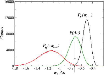
Figure 2: (Color on line) Example of histograms corresponding to $P_{F}(w_{0\rightarrow 1})$, $P_{R}(-w_{1\rightarrow 0})$ and $P(\Delta u)$. The arrow pointing downwards indicates the position of the maximum of $P(\Delta u)$ and the arrow pointing upwards the average value $\langle\Delta u\rangle$. The example corresponds to a system with $\sigma=4$, $H_{1}=-0.35$ and $L=12$. Histograms have been obtained by cumulating data corresponding to $4\times 10^{5}$ realizations of disorder.

III First strategy

Fig. 2 shows histograms corresponding to the distributions of $w_{0\rightarrow 1}$, $\Delta u$ and $-w_{1\rightarrow 0}$ for $\sigma=4$, $H_{1}=-0.35$ and a system size $L=12$. The computed histograms give an estimation of the corresponding probability densities $P_{F}(w_{0\rightarrow 1})$, $P_{R}(-w_{1\rightarrow 0})$ and $P(\Delta u)$. Four important points should be realized from this example: (i) For this value of $\sigma$ and field $H_{1}$, the densities look symmetric and Gaussian. This will not be the case when $H_{1}$ and $\sigma$ are close to the disorder induced phase transition at $\sigma_{c}^{eq}$ and $H_{1}=0$. (ii) Second, the distribution of $\Delta u$ has a width similar to those of the out-of-equilibrium works. This is different from what happens in the analysis of Crooks fluctuation theorem at finite $T$. Typically, equilibrium thermal fluctuations are much smaller than work fluctuations. (iii) For increasing systems size the histograms become narrower and then the crossing points are harder to locate (iv) Finally, note that for this case the hypothesis that we are testing is fulfilled: the peak in $P(\Delta u)$ as well as the average $\langle\Delta u\rangle$ coincide with the crossing point $w^{*}$ of $P_{F}(w_{0\rightarrow 1})$ and $P_{R}(-w_{1\rightarrow 0})$.

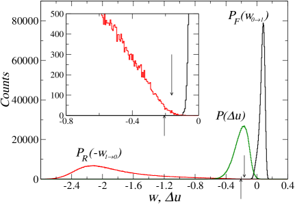
Figure 3: (Color on line) Example of histograms corresponding to $P_{F}(w_{0\rightarrow 1})$, $P_{R}(-w_{1\rightarrow 0})$ and $P(\Delta u)$. The arrow pointing downwards indicates the position of the maximum of $P(\Delta u)$ and the arrow pointing upwards the average value $\langle\Delta u\rangle$. The example corresponds to a system with $\sigma=3$, $H_{1}=0.1$ and $L=12$. The histograms have been computed by cumulating data corresponding to $1.6\times 10^{6}$ realizations of disorder. The inset shows a detailed view of the crossing point of the $P_{F}(w_{0\rightarrow 1})$ and $P_{R}(-w_{1\rightarrow 0})$ histograms.

Figure 4: Schematic representation of the case $\sigma\lesssim\sigma_{c}^{eq}$ and $H_{1}>0$. Dashed lines correspond to metastable trajectories, continuous lines to the equilibrium trajectory and the dashed-dotted line to the non typical equilibrium states that are responsible for the high asymmetry of the distribution $P_{R}(-w_{1\rightarrow 0})$.

Fig. 3 shows histograms corresponding to $P(w_{0\rightarrow 1})$, $P(\Delta u)$ and $P(-w_{1\rightarrow 0})$ for $\sigma=3$, $H_{1}=0.1$ and a system size $L=12$. Note than in this case, the work distributions as well as the energy distribution are very asymmetric. This is because although in this case we expect $M_{1}>0$ since $H_{1}>0$, a certain non vanishing fraction of the equilibrium states still has $M_{1}<0$, as schematically indicated in Fig.4. In other words, for certain realizations of disorder, the state $1$ turns out to be non-typical and previous to the equilibrium transition from $M<0$ to $M>0$. Consequently, the distribution of reverse works $w_{1\rightarrow 0}$ widens enormously. As can be seen the proposed equality $w^{*}=\Delta u$ clearly fails in this case. The relative error is $|w^{*}-\langle\Delta u\rangle|/|\langle\Delta u\rangle|\sim 0.25$.

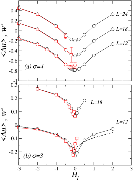
Figure 5: (Color on line) Comparison of the crossing point of the histograms $w^{*}$ ($\Box$) with $\langle\Delta u\rangle$ ($\Circle$) as a function of $H_{1}$, corresponding to (a) $\sigma=4$ and (b) $\sigma=3$ for different values of $L$ as indicated by the legend. For the case $L=12$ and $\sigma=3$ the dashed line indicated the position of the maximum of $P(\Delta u)$. Data for $L=18$ ($L=24$) has been shifted 0.3 (0.6) units along the vertical axis in order to clarify the picture.

We have performed a detailed study of the deviation of $w^{*}$ from $\langle\Delta u\rangle$ for different values of $\sigma$, $H_{1}$ and $L$. Examples of the results are presented in Fig. 5. Note that the data corresponding to the crossing point $w^{*}$ exhibits increasing error bars with increasing $H_{1}$. This is because the histograms of $P_{F}(w_{0\rightarrow 1})$, $P_{R}(-w_{1\rightarrow 0})$ become more and more separated and the finding of the intersection requires more and more statistics. (This problem is accentuated for larger values of $H_{1}$ and for larger system sizes). One can conclude therefore than the proposed extrapolation of Crooks theorem, given by the equality $w^{*}=\langle\Delta u\rangle$ fails in the region of $\sigma$ and $H_{1}$ where the system exhibits a collective behaviour (i.e. the correlation length is similar to the system size) because of the proximity of the equilibrium phase transition. Consistently, we observe in Fig. 5(b) (comparing the data corresponding to $L=12$ and $L=18$ at $H_{1}\sim 0$) that the region of breakdown becomes smaller when the system size $L$ is larger. As expected, increasing the system size with fixed correlation length decreases the collective effects.

IV Second strategy

Fig. 6 shows histograms corresponding to the distributions of $v_{0\rightarrow 1}$ and $-v_{1\rightarrow 0}$ for the case $L=12$, $\sigma=3$, $H_{1}=-10$ and $H_{2}=-0.4$. As can be seen the intersection point $v^{*}$ agrees very well with the average value of $\Delta u-\Delta(Hm)$. In this case we have also studied if this agreement is equally good in other regions of the phase diagram.

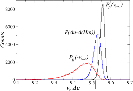
Figure 6: (Color on line) Example of histograms corresponding to $P_{F}(v_{0\rightarrow 1})$, $P_{R}(-v_{1\rightarrow 0})$ and $P\left(\Delta u-\Delta(Hm)\right)$. Data corresponds to $H_{0}=-10.0$,$H_{1}=-0.4$, $\sigma=3$ and $L=12$. Histograms are computed by cumulating $10^{5}$ realizations of disorder. The arrows pointing down (up) indicate the peak (average value) of the distribution $P(\Delta u-\Delta(HM))$.

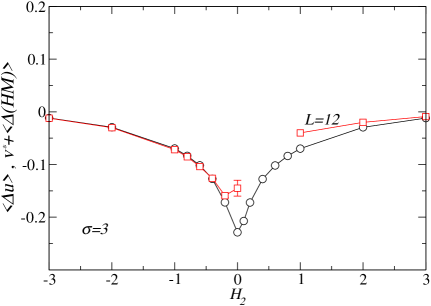
Figure 7: (Color on line) Comparison of the crossing point $v^{*}$ ($\Box$) of the histograms $P_{F}(v_{0\rightarrow 1})$ and $P_{R}(-v_{1\rightarrow 0})$ with $\langle\Delta u-\Delta(Hm)\rangle$ ($\Circle$) as a function of $H_{2}$, corresponding to $\sigma=3$ and $L=12$. Data corresponds to averages over $10^{5}$ realizations of disorder

Fig 7 shows a comparison of $\langle\Delta u\rangle$ and $v^{*}+\langle\Delta(Hm)\rangle$. On the right hand side, the value of $v^{*}$ has not been obtained by a direct location of the intersection of the histograms but locating the mid point between the positions of the maxima of the histograms corresponding to $P_{F}(v_{0\rightarrow 1})$ and $P_{R}(-v_{1\rightarrow 0})$ which are far separated but very symmetric. As can be seen, as occurs with strategy 1, the agreement $v^{*}\simeq\langle\Delta u-\Delta(Hm)\rangle$ fails when $H_{2}$ approaches the phase transition region.

V Summary and conclusion

We have investigated the possibility of extending some work fluctuation theorems to $T=0$ for systems with quenched disorder. In this case, thermal averages should be substituted by disorder averages. We have proposed an hypothesis based on the extrapolation of Crooks theorem to the $T\rightarrow 0$ limit and we have numerically tested its validity. The hypothesis is that if one considers the distributions of non-equilibrium work corresponding to a forward and backwards trajectory, the crossing point $w^{*}$ of $P_{F}(w_{0\rightarrow 1})$ and $P_{R}(-w_{1\rightarrow 0})$, is equal to the average of the internal energy difference $\Delta u=u_{1}-u_{2}$. The investigation has been done by considering two strategies, based on the two possible definitions of work that have been discussed in the literature: $w=\int Hdm$ and $v=\int mdH$.

The reported numerical investigation indicates that, for both strategies, the formulated hypothesis is valid when the system does not behave collectively. Thus, far from the equilibrium critical point, where correlations are small compared to system size, the distribution $p(\Delta u)$ is very symmetric and the average (equilibrium) value $\langle\Delta u\rangle$ can be obtained from the crossing point $w^{*}$ of the distributions of the non equilibrium works.

When the system is close to the critical point a definitive conclusion can not be stated. Data for small $L$ suggest that when the correlation length approaches the system size $L$, the distribution $p(\Delta u)$ is very assymetric and there is no connection between the equilibrium value $\langle\Delta u\rangle$ and the crossing point $w^{*}$ of the non-equilibrium work distributions. A bigger computational effort (not affordable at present) would be needed in order to compute the accurate histograms for $L>24$. The presented results may provide some clues for future investigations in order to extend work fluctuation theorems.