A Construction of Biorthogonal Wavelets With a Compact Operator

Abstract

We present a construction of biorthogonal wavelets using a compact operator which allows to preserve or increase some properties: regularity/vanishing moments, parity, compact supported. We build then a simple algorithm which computes new filters.

1 Introduction

The aim of this paper is to present a construction of biorthogonal wavelets with some properties of vanishing moments/regularity which could be a powerful tool in wavelet partial differential equations theory ; in particular in the case of the wavelet-Galerkin method (WG)(see e.g [1]) or the so-called hybrid method ([2, 5]). The property of regularity/vanishing moment is more important in wavelets theory. To this end, we use an iterative process to get new wavelets. The new wavelets have $s$ vanishing moments while the biorthogonal ones are more regular. Moreover, this construction could be a way to recover all boxed spline wavelets. As in most works, we privilege compactly supported wavelets which are very attractive for such a construction.
We present in the following section a way to construct these wavelets using a simple compact operator. To this end, we choose initially biorthogonal wavelets (orthonormal wavelets can also be choose) and we define them from the so-called transfer functions. We show how to build easily theirs discrete filters in practice. In what follows, we denote by: BMRA biorthogonal multi-resolution analysis, OMRA orthogonal multi-resolution analysis, ($\phi,\,\psi$) initial scaling function-wavelet pair with ($\widetilde{\phi},\,\widetilde{\psi}$) the dual pair, ($\Phi^{(s)},\,\Psi^{(s)}$) the constructed scaling function-wavelet pair at order $s$ where $s$ design the vanishing moments (or degree of approximation) with ($\widetilde{\Phi}^{(s)},\,\widetilde{\Psi}^{(s)}$) the dual pair where $s$ denotes the order of regularity and $\langle\cdot\,,\,\cdot\rangle$ denotes the usual scalar product of $L^{2}(\mathbb{R})$. We denote also by (TSR) the classical two scale relation

2 Main results

Our motivation is to construct a high order method to elevate the degree of vanishing moment and regularity of any given biorthogonal wavelet in order to get powerful wavelets for wavelet partial differential equations theory. For this purpose, let us introduce the compact operator $T$ of kernel $G(x,y)=\mathds{1}_{[x-1,x]}(y)$ where its adjoint is defined by $G^{*}(x,y)=\mathds{1}_{[x,x+1]}(y)$. The operator $T$ acting $s$ times on the initial wavelet is an elegant way to build a new pair of biorthogonal wavelets. The process is called an elevation at order $s$. To start the construction, we choose initially biorthogonal wavelets.

Theorem 1

Let $\phi$, $\tilde{\phi}$ be two scaling functions of a BMRA. Let $T$ be the operator described above and $T^{*}$ its adjoint. Let $s\in\mathbb{N}$ be the order of elevation and let us define $\Phi^{(s)}$ and $\tilde{\Phi}^{(s)}$ as

$$\Phi^{(s)}:=(T)^{s}\phi,\quad\tilde{\Phi}^{(s)}:=\left(T^{*}\right)^{-s}\tilde{\phi}$$

where $(X)^{s}$ designs the action of $X$ $s$ times, and by definition $X^{0}:=Id$.
Then, the scaling functions $\Phi^{(s)}$ and $\tilde{\Phi}^{(s)}$ generates a BMRA. Moreover,

$$P_{0}^{(s)}(w)=\frac{1}{2^{s}}\frac{S_{s}(2w)}{S_{s}(w)}m_{0}(w),\,\tilde{P}_{0}^{(s)}(w)=2^{s}\frac{\overline{S_{s}(w)}}{\overline{S_{s}(2w)}}\tilde{m}_{0}(w)$$

$$P_{1}^{(s)}(w)=2^{s}\frac{m_{1}(w)}{S_{s}(w)},\,\tilde{P}_{1}^{(s)}(w)=\frac{1}{2^{s}}\overline{S_{s}(w)}\tilde{m}_{1}(w)$$

where $m_{0}$, $\tilde{m}_{0}$, $P_{0}^{(s)}$, $\tilde{P}_{0}^{(s)}$, $m_{1},\,\tilde{m}_{1}$, $P_{1}^{(s)}$, $\tilde{P}_{1}^{(s)}$ denote the transfer functions of $\phi$, $\tilde{\phi}$, $\Phi^{(s)}$, $\tilde{\Phi}^{(s)}$, $\psi$, $\tilde{\psi}$, $\Psi^{(s)}$, $\tilde{\Psi}^{(s)}$ and $S_{s}(w)=(1-e^{-iw})^{s}.$

To prove Theorem 1, let us recall the following results:

Lemma 2

Let $\phi$ be a scaling function then

$(i)$

$\Gamma>0$ where $\Gamma(w)=\displaystyle\sum_{k\in\mathbb{Z}}|\hat{\Phi}(w+2k\pi)|^{2}$.

$(ii)$

The set $\{\Phi(.-k),\,k\in\mathbb{Z}\}$ forms a Riesz basis.

Lemma 3

Let $(\phi,\psi)$ be the scaling function and wavelet of an OMRA. We suppose $\phi$, $\psi$ differentiable. Then the following equality holds

$$\langle\psi^{\prime}(x),\psi^{\prime}(x-k)\rangle+\langle\phi^{\prime}(x),\phi^{\prime}(x-k)\rangle=4\langle\phi^{\prime}(x),\phi^{\prime}(x-2k)\rangle\,.$$

In order to complete the proof let us do the following remark.

Remark 2.1

We have:

$$\Psi(x)=4\int_{-\infty}^{x}\psi(t)dt,\,\,\,4\int_{-\infty}^{x}\tilde{\Psi}(t)dt=\psi(x),\,\,\,\forall x\in\mathbb{R}.$$ (1)

Proof of theorem 1: For $s=0$, the results holds since we get the classical definition of the transfer functions. For $s=1$, see e.g. [3]. For $s>1$, let us denote to simplify notations $\phi=\Phi^{(s)}$ and $\Phi=\Phi^{(s+1)}$.
We show firstly that the set $\{\Phi(\cdot-k),\,k\in\mathbb{Z}\}$ cannot be orthonormal and thus there exists a biorthogonal function denoted by $\tilde{\Phi}$. To this end, we proceed as follows:

Step $1$.

$\Phi$ satisfies a the (TSR). Indeed, since

$$\Phi(x)=T\phi(x)=\int_{-\infty}^{x}\left(\phi(t)-\phi(t-1)\right)dt$$

and using the (TSR) on $\phi$. Furthermore, when $\mbox{\rm{supp }}\phi^{(s)}=[0,2p-1+s]$, we obtain the discrete filters of $\Phi$ defined as:

$$H_{k}=\displaystyle\frac{h_{k-1}+h_{k}}{2},\,k=0\ldots 2p\textrm{ with }h_{-1}=h_{2p}=0.$$

Step $2$.

Now, it remains to show that $(\Phi(\cdot-k))_{k\in\mathbb{Z}}$ forms a Riesz basis. For this purpose, we use Lemma 2 to find two constants $0<A\leq B$ such that

$$\forall w\in\mathbb{R},\,\displaystyle A\leq\sum_{k\in\mathbb{Z}}|\hat{\Phi}(w+2k\pi)|^{2}\leq B.$$

The fact that $\Gamma$ is $2\pi$-periodic continuous with compacity property give us the constant $B$ whereas $A$ is obtained since $\Gamma>0$.

Step $3$.

To conclude, we prove that $(\Phi(\cdot-k))_{k\in\mathbb{Z}}$ never forms an orthonormal family but it satisfy $\displaystyle\langle\Phi(\cdot-k),\Phi(\cdot)\rangle=0$ for almost all integer $k$ which ensures that the family $\Phi$ cannot be orthonormal. This is done by setting $\tilde{\phi}=T^{\ast}\tilde{\Phi}$ and using Property (1), Lemma 3. The transfer functions are obtained by a straightforward computation.

When $\phi,\,\tilde{\phi}$ are compactly supported, we have:

Theorem 4

Under the hypothesis of theorem 1, if we suppose that $\phi$ and $\tilde{\phi}$ are compactly supported where $\mbox{\rm{supp }}\phi=[0,2p-1]$ and $\mbox{\rm{supp }}\tilde{\phi}=[0,2\tilde{p}-1]$ then writing $H_{k}^{(s)}$, $\tilde{H}_{k}^{(s)}$ the discrete filters of $\Phi^{(s)}$, $\tilde{\Phi}^{(s)}$ (resp.) and $h_{k}^{(s)}$, $\tilde{h}_{k}^{(s)}$ the discrete filters of $\phi^{(s)}$, $\tilde{\phi}^{(s)}$ we have,

$$\begin{array}[]{lll}\mbox{\rm{supp }}\Phi^{(s)}&=&[0,2p-1+s]\\ \mbox{\rm{supp }}\tilde{\Phi}^{(s)}&=&[0,2\tilde{p}-1-s]\end{array}$$

with the following formulas to compute the new filters from the older

$$\begin{array}[]{lll}H_{k}^{(s)}=\displaystyle\frac{1}{2^{s}}\sum_{l=0}^{s}\left(\begin{array}[]{c}s\\ l\end{array}\right)h_{k-l},&k=0\ldots 2p-1+s\end{array}$$ (2)

$$\begin{array}[]{lll}\displaystyle\sum_{l=0}^{s}\left(\begin{array}[]{c}s\\ l\end{array}\right)\tilde{H}^{(s)}_{k-l}=2^{s}\tilde{h}_{k},&k=0\ldots 2\tilde{p}-1-s,\,\tilde{p}\geq\displaystyle\frac{s+1}{2}\end{array}$$ (3)

Proof of Theorem 4: We have already proved the result for $s=1$ (Step $1$. of the proof of Theorem 1). Writing $H_{k}^{0}:=h_{k}$, we have

for $s=1$:

$\displaystyle H_{k}^{(1)}=\frac{H^{(0)}_{k-1}+H^{(0)}_{k}}{2}$ and $\displaystyle\Phi^{(1)}$ admits an approximation of degree $p+1$ and $\mbox{\rm{supp }}\displaystyle\Phi^{(1)}=[0,2p]$.

for $s=2$:

$H_{k}^{(2)}=\displaystyle\frac{H^{(1)}_{k-1}+H^{(1)}_{k}}{2}$ and $\displaystyle\Phi^{(2)}$ admits an approximation of degree $p+2$ and $\mbox{\rm{supp }}\displaystyle\Phi^{(1)}=[0,2p+1]$. In addition, according to the step $s=1$, we can rewrite:

$$H_{k}^{(2)}=\displaystyle\frac{H^{(0)}_{k}+H^{(0)}_{k-1}+H^{(0)}_{k-1}+H^{(0)}_{k-2}}{2^{2}}.$$

The result for $s>2$ is obtained by replacing $\Phi^{(s)},\,\tilde{\Phi}^{(s)}$ by $\Phi^{(s+1)},\,\tilde{\Phi}^{(s+1)}$ and applying succesively the result for $s=1$.

The dual discrete filters are obtained by substituting $h_{k}$ by $\tilde{H}_{k}$ and $\tilde{h}_{k}$ by $H_{k}$ with Property (1).$\square$
We conclude with some representation of wavelets in the biorthogonal and orthonormal cases:

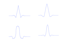
Figure 1: Top left $\phi$, top right $\tilde{\phi}$, bottom left $\Phi^{(1)}$, bottom right $\tilde{\Phi}^{(1)}$ where $\phi,\tilde{\phi}$ are compactly supported B-spline 4 4

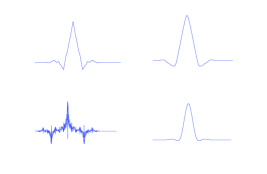
Figure 2: Top left $\phi$, top right $\tilde{\phi}$, bottom left $\Phi^{(2)}$, bottom right $\tilde{\Phi}^{(2)}$ where $\phi,\tilde{\phi}$ are compactly supported B-spline 4 4

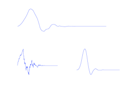
Figure 3: Top left $\phi$, bottom left $\Phi^{(1)}$, bottom right $\tilde{\Phi}^{(1)}$ where $\phi$ is the Daubechies Wavelet with $4$ vanishing moments

3 Conclusion

The constructed wavelet $\tilde{\Phi}^{(s)}$ is more regular than $\Phi^{(s)}$ but has less vanishing moments. We have gained vanishing moments for one and regularity for the other but in counterpart we have increased the support of the scaling function but still compact. This operation preserves the parity of the initial wavelet and if initial wavelets are curl free then so are the constructed wavelets. Moreover, this construction is a way to recover all boxed splines. We have also a similar way to construct biorthogonal wavelets from an orthonormal initial family defining $\widetilde{\Phi}^{(s)}=\left(T^{\star}\right)^{(s)}\phi$.

References

• [1] K. Amaratunga, J.R. Williams, S. Qian, and J. Weiss. Wavelet-Galerkin solutions for one-dimensional partial differential equations. Int. J. Num. Meth. Eng., 37(16):2703–2716, 1994.
• [2] J. Fröhlich and K. Schneider. An adaptive wavelet-vaguelette algorithm for the solution of PDEs. J. Comput. Phys., 130(2):174–190, 1997.
• [3] P.G. Lemarié-Rieusset. Analyse multi-résolutions non orthogonales, commutation entre projéjecteurs et dérivation et ondelettes vecteurs à divergence nulle. Revista Matemática Iberoamericana 8(2): 221-236, 1992.
• [4] S. Mallat. A Wavelet Tour of Signal Processing, Second Edition (Wavelet Analysis & Its Applications) Academic Press, 1999
• [5] Pj Ponenti and J. Liandrat. Numerical algorithms based on biorthogonal wavelets. Technical Report 96-13, Institute for Computer Applications in Science and Engineering (ICASE), 1996.