Fast rotating Bose-Einstein condensates in an asymmetric trap

Abstract.

We investigate the effect of the anisotropy of a harmonic trap on the behaviour of a fast rotating Bose-Einstein condensate. This is done in the framework of the 2D Gross-Pitaevskii equation and requires a symplectic reduction of the quadratic form defining the energy. This reduction allows us to simplify the energy on a Bargmann space and study the asymptotics of large rotational velocity. We characterize two regimes of velocity and anisotropy; in the first one where the behaviour is similar to the isotropic case, we construct an upper bound: a hexagonal Abrikosov lattice of vortices, with an inverted parabola profile. The second regime deals with very large velocities, a case in which we prove that the ground state does not display vortices in the bulk, with a 1D limiting problem. In that case, we show that the coarse grained atomic density behaves like an inverted parabola with large radius in the deconfined direction but keeps a fixed profile given by a Gaussian in the other direction. The features of this second regime appear as new phenomena.

1. Introduction

Bose-Einstein condensates (BEC) are a new phase of matter where various aspects of macroscopic quantum physics can be studied. Many experimental and theoretical works have emerged in the past ten years. We refer to the monographs by C.J.Pethick-H.Smith [17], L.Pitaevskii-S.Stringari [18] for more details on the physics and to A.Aftalion [2] for the mathematical aspects. Our work is motivated by experiments in the group of J.Dalibard [14] on rotating condensates: when a condensate is rotated at a sufficiently large velocity, a superfluid behaviour is detected with the observation of quantized vortices. These vortices arrange themselves on a lattice, similar to Abrikosov lattices in superconductors [1]. This fast rotation regime is of interest for its analogy with Quantum Hall physics [5, 9, 21].

In a previous work, A.Aftalion, X.Blanc and F.Nier [3] have addressed the mathematical aspects of fast rotating condensates in harmonic isotropic traps and gave a mathematical description of the observed vortex lattice. This was done through the minimization of the Gross-Pitaevskii energy and the introduction of Bargmann spaces to describe the lowest Landau level sets of states. Nevertheless, the experimental device leading to the realization of a rotating condensate requires an anisotropy of the trap holding the atoms, which was not taken into account in [3]. Several physics papers have addressed the behaviour of anisotropic condensates under rotation and its similarity or differences with isotropic traps. We refer the reader to the paper by A.Fetter [8], and to the related works [16, 19, 20]. The aim of the present article is to analyze the effect of anisotropy on the energy minimization and the vortex pattern, and in particular to derive a mathematical study of some of Fetter’s computations and conjectures. Two different situations emerge according to the values of the parameters: in one case, the behaviour is similar to the isotropic case with a triangular vortex lattice; in the other case, for very large velocities, we have found a new regime where there are no vortices, and a full mathematical analysis can be performed, reducing the minimization to a 1D problem. The existence of this new regime was apparently not predicted in the physics literature. This feature relies on the analysis of the bottom of the spectrum of a specific operator whose positive lower bound prevents the condensate from shrinking in one direction, contradicting some heuristic explanations present in [8]. Our analysis is based on the symplectic reduction of the quadratic form defining the Hamiltonian (inspired by the computations of Fetter [8]), the characterization of a lowest Landau level adapted to the anisotropy and finally the study of the reduced energy in this space.

1.1. The physics problem and its mathematical formulation

Our problem comes from the study of the 3D Gross-Pitaevskii energy functional for a fast rotating Bose-Einstein condensate with $N$ particles of mass $m$ given by

(1.1) $$\mathcal{E}_{GP}(\phi)=\langle\mathcal{H}\phi,\phi\rangle_{L^{2}(\mathbb{R}^{3})}+\frac{g_{3d}N}{2}\|\phi\|^{4}_{L^{4}(\mathbb{R}^{3})},$$

where the operator $\mathcal{H}$ is

(1.2) $$\mathcal{H}=\frac{1}{2m}(h^{2}D_{x}^{2}+h^{2}D_{y}^{2}+h^{2}D_{z}^{2})+\frac{m}{2}\bigl{(}\omega_{x}^{2}x^{2}+\omega_{y}^{2}y^{2}+\omega_{z}^{2}z^{2}\bigr{)}-\Omega(xhD_{y}-yhD_{x}),$$

where $h$ is the Planck constant, $D_{x}=(2i\pi)^{-1}\partial_{x}$, $\omega_{j}$ is the frequency along the $j$-axis, $\Omega$ is the rotational velocity, and the coupling constant $g_{3d}$ is a positive parameter.

In the particular case where $\omega_{x}=\omega_{y}$, the fast rotation regime corresponds to the case where $\Omega$ tends to $\omega_{x}$ and the condensate expands in the transverse direction. It has been proved [4] that the minimizer can be described at leading order by a 2D function $\psi(x,y)$, multiplied by the ground state of the harmonic oscillator in the $z$-direction (the operator $h^{2}/(2m)D_{z}^{2}+m\omega_{z}^{2}z^{2}/2$), which is equal to $({2m\omega_{z}h^{-1}})^{1/4}e^{-\pi m\omega_{z}h^{-1}z^{2}}.$ This property is still true in the anisotropic case if $\omega_{y}\ll\omega_{z}$. The reduced 2D energy to study is thus

(1.3) $$\mathcal{E}(\psi)=\langle\mathcal{H}_{0}\psi,\psi\rangle_{L^{2}(\mathbb{R}^{2})}+\frac{g_{2d}N}{2}\|\psi\|^{4}_{L^{4}(\mathbb{R}^{2})},$$

where the operator $\mathcal{H}_{0}$ is

(1.4) $$\mathcal{H}_{0}=\frac{1}{2m}(h^{2}D_{x}^{2}+h^{2}D_{y}^{2})+\frac{m}{2}\bigl{(}\omega_{x}^{2}x^{2}+\omega_{y}^{2}y^{2}\bigr{)}-\Omega(xhD_{y}-yhD_{x}),$$

and the coupling constant $g_{2d}$ takes into account the integral of the ground state in the $z$-direction:

(1.5) $$g_{2d}N=\frac{gh^{2}}{m},\quad\text{where $g$ is dimensionless (and $>0$).}$$

Since $h$ has the dimension energy $\times$ time, it is consistent to assume that the wave function $\psi$ has the dimension 1/length, with the normalization $\|\psi\|_{L^{2}(\mathbb{R}^{2})}=1.$ We define the mean square oscillator frequency $\omega_{\perp}$ by

$$\omega_{\perp}^{2}=\frac{1}{2}(\omega_{x}^{2}+\omega_{y}^{2})$$

and the function $u$ by

(1.6) $$\psi(x,y)=h^{-1/2}m^{1/2}\omega_{\perp}^{1/2}u(h^{-1/2}m^{1/2}\omega_{\perp}^{1/2}x,h^{-1/2}m^{1/2}\omega_{\perp}^{1/2}y),$$

so that

$$\|u\|_{L^{2}(\mathbb{R}^{2})}=\|\psi\|_{L^{2}(\mathbb{R}^{2})}=1,\quad g_{2d}N\|\psi\|_{L^{4}(\mathbb{R}^{2})}^{4}=gh\omega_{\perp}\|u\|_{L^{4}(\mathbb{R}^{2})}^{4}.$$

We also note that the dimension of $h^{-1/2}m^{1/2}\omega_{\perp}^{1/2}$ is 1/length, so that

$$x_{1}=h^{-1/2}m^{1/2}\omega_{\perp}^{1/2}x,\quad x_{2}=h^{-1/2}m^{1/2}\omega_{\perp}^{1/2}y,\quad u(x_{1},x_{2})\quad\text{are dimensionless.}$$

Assuming $\omega_{x}^{2}\leq\omega_{y}^{2}$, we use the dimensionless parameter $\nu$ to write

$$\omega_{x}^{2}=(1-\nu^{2})\omega_{\perp}^{2},\quad\omega_{y}^{2}=(1+\nu^{2})\omega_{\perp}^{2},$$

and we get immediately

$$\frac{1}{h\omega_{\perp}}\mathcal{E}(\psi)=\frac{1}{2}\|D_{1}u\|_{L^{2}(\mathbb{R}^{2})}^{2}+\frac{1}{2}\|D_{2}u\|_{L^{2}(\mathbb{R}^{2})}^{2}+\frac{1}{2}(1-\nu^{2})\|x_{1}u\|_{L^{2}(\mathbb{R}^{2})}^{2}+\frac{1}{2}(1+\nu^{2})\|x_{2}u\|_{L^{2}(\mathbb{R}^{2})}^{2}\\ -\frac{\Omega}{\omega_{\perp}}\langle(x_{1}D_{2}-x_{2}D_{1})u,u\rangle_{L^{2}(\mathbb{R}^{2})}+\frac{g}{2}\|u\|_{L^{4}(\mathbb{R}^{2})}^{4}.$$

Finally, we have

(1.7) $$\frac{1}{h\omega_{\perp}}\mathcal{E}(\psi):=E_{GP}(u)=\langle Hu,u\rangle+\frac{g}{2}\|u\|_{L^{4}(\mathbb{R}^{2})}^{4},$$

(1.8) $$2H=D_{1}^{2}+D_{2}^{2}+(1-\nu^{2})x_{1}^{2}+(1+\nu^{2})x_{2}^{2}-2\omega(x_{1}D_{2}-x_{2}D_{1}),\quad\omega=\frac{\Omega}{\omega_{\perp}},$$

where $\omega,\nu,u,g$ are all dimensionless and $\|u\|_{L^{2}(\mathbb{R}^{2})}=1$. The minimization of this functional is the mathematical problem that we address in this paper. The Euler-Lagrange equation for the minimization of $E_{GP}(u)$, under the constraint $\|u\|_{L^{2}(\mathbb{R}^{2})}=1$, is

(1.9) $$Hu+g|u|^{2}u=\lambda u,$$

where $\lambda$ is the Lagrange multiplier. We shall always assume that $\Omega^{2}\leq\omega_{x}^{2},$ i.e. $\omega^{2}+\nu^{2}\leq 1$ and define the dimensionless parameter $\varepsilon$ by

(1.10) $$\omega^{2}+\nu^{2}+\varepsilon^{2}=1.$$

The fast rotation regime occurs when the ratio $\Omega^{2}/\omega_{x}^{2}$ tends to $1_{-}$, i.e. $\varepsilon$ tends to 0.

Summarizing and reformulating our reduction, we have

(1.11) $$E_{GP}(u)=\frac{1}{2}\langle q_{\omega,\nu,\varepsilon}^{w}u,u\rangle_{L^{2}(\mathbb{R}^{2})}+\frac{g}{2}\int_{\mathbb{R}^{2}}|u|^{4}dx,$$

where $q_{\omega,\nu,\varepsilon}$ is the quadratic form

(1.12) $$q_{\omega,\nu,\varepsilon}(x_{1},x_{2},\xi_{1},\xi_{2})=\xi_{1}^{2}+\xi_{2}^{2}+(1-\nu^{2})x_{1}^{2}+(1+\nu^{2})x_{2}^{2}-2\omega(x_{1}\xi_{2}-x_{2}\xi_{1}),$$

which depends on the real parameters $\omega,\nu,\varepsilon$ such that (1.10) holds. Here $q^{w}_{\omega,\nu,\varepsilon}$ is the operator with Weyl symbol $q_{\omega,\nu,\varepsilon},$ that is:

(1.13) $$q^{w}_{\omega,\nu,\varepsilon}=D_{1}^{2}+D_{2}^{2}+(1-\nu^{2})x_{1}^{2}+(1+\nu^{2})x_{2}^{2}-2\omega(x_{1}D_{2}-x_{2}D_{1}),$$

where $D_{j}=\partial_{j}/(2i\pi).$ We would like to minimize the energy $E_{GP}(u)$ under the constraint $\|u\|_{L^{2}}=1$ and understand what is happening when $\varepsilon\rightarrow 0$.

1.2. The isotropic Lowest Landau Level

When the harmonic trap is isotropic, i.e. when $\nu=0$, it turns out that, since $\omega^{2}+\varepsilon^{2}=1$,

(1.14) $$q=q_{\omega,0,\varepsilon}=(\xi_{1}+\omega x_{2})^{2}+(\xi_{2}-\omega x_{1})^{2}+\varepsilon^{2}(x_{1}^{2}+x_{2}^{2})$$

so that

$$E_{GP}(u)=\frac{1}{2}\|(D_{1}+\omega x_{2})\psi+i(D_{2}-\omega x_{1})u\|^{2}+\frac{\omega}{2\pi}\|u\|^{2}+\frac{\varepsilon^{2}}{2}\||x|u\|^{2}+\frac{g}{2}\int|u|^{4}dx.$$

We note that, with $z=x_{1}+ix_{2}$,

$$D_{1}+\omega x_{2}+i(D_{2}-\omega x_{1})=\frac{1}{i\pi}\bar{\partial}-i\omega z=\frac{1}{i\pi}(\bar{\partial}+\pi\omega z),$$

hence the first term of the energy is minimized (and equal to $0$) if $u\in LLL_{\omega^{-1}}$, where

(1.15) $$LLL_{\omega^{-1}}=\{u\in L^{2}(\mathbb{R}^{2}),u(x)=f(z)e^{-\pi\omega|z|^{2}}\}=\ker(\bar{\partial}+\pi\omega z)\cap L^{2}(\mathbb{R}^{2}),$$

with $f$ holomorphic. We expect the condensate to have a large expansion, hence the term $\int|u|^{4}$ to be small. Thus, it is natural to minimize the energy $E_{GP}$ in $LLL_{\omega^{-1}}.$ It has been proved in [4] that the restriction to $LLL_{\omega^{-1}}$ is a good approximation of the original problem, i.e. the minimization of $E_{GP}$ in $L^{2}(\mathbb{R}^{2})$. We get for $u\in LLL_{\omega^{-1}},\|u\|_{L^{2}}=1,$

$$E_{GP}(u)=\frac{1}{2}\|\underbrace{(D_{1}+\omega x_{2})u+i(D_{2}-\omega x_{1})u}_{(i\pi)^{-1}(\bar{\partial}+\pi\omega z)u=0}\|^{2}+\frac{\omega}{2\pi}+\frac{\varepsilon^{2}}{2}\||x|u\|^{2}+\frac{g}{2}\int|u|^{4}dx,$$

and with $u(x)=\upsilon\bigl{(}(\omega\varepsilon)^{1/2}x\bigr{)}(\omega\varepsilon)^{1/2}$ (unitary change in $L^{2}(\mathbb{R}^{2})$),

$$E_{GP}(u)=\frac{\omega}{2\pi}+\frac{\varepsilon}{2\omega}\left(\int|y|^{2}|\upsilon(y)|^{2}dy+{\omega^{2}g}\int{|\upsilon(y)|}^{4}dy\right).$$

The minimization problem of $E_{GP}(u)$ in the space $LLL_{\omega^{-1}}$ is thus reduced to study

(1.16) $$E_{LLL}(\upsilon)=\||x|\upsilon\|^{2}_{L^{2}}+\omega^{2}g\|\upsilon\|^{4}_{L^{4}},\quad\upsilon\in LLL_{\varepsilon},$$

i.e. with $z=x_{1}+ix_{2}$, $v(x_{1},x_{2})=f(z)e^{-\pi\varepsilon^{-1}|z|^{2}},$ $f$ entire (and $v\in L^{2}(\mathbb{R}^{2})$). This program has been carried out in the paper [3] by A. Aftalion, X. Blanc, F. Nier. In the isotropic case, a key point is the fact that the symplectic diagonalisation of the quadratic Hamiltonian is rather simple: in fact revisiting the formula (1.14), we obtain easily

(1.17) $$q=\overbrace{(\frac{1-\omega}{2})(\xi_{1}-x_{2})^{2}}^{\eta_{1}^{2}}+\overbrace{(\frac{1-\omega}{2})(\xi_{2}+x_{1})^{2}}^{\mu_{1}^{2}y_{1}^{2}}\\ +\underbrace{(\frac{1+\omega}{2})(\xi_{1}+x_{2})^{2}}_{\eta_{2}^{2}}+\underbrace{(\frac{1+\omega}{2})(\xi_{2}-x_{1})^{2}}_{\mu_{2}^{2}y_{2}^{2}},$$

with

(1.18) $$\left\{\begin{matrix}\eta_{1}=2^{-1/2}(1-\omega)^{1/2}(\xi_{1}-x_{2}),&\mu_{1}=1-\omega,&y_{1}=2^{-1/2}(1-\omega)^{-1/2}(\xi_{2}+x_{1}),\\ \\ \eta_{2}=2^{-1/2}(1+\omega)^{1/2}(\xi_{1}+x_{2}),&\mu_{2}=1+\omega,&y_{2}=2^{-1/2}(1+\omega)^{-1/2}(x_{1}-\xi_{2}),\end{matrix}\right.$$

so that the linear forms $(y_{1},y_{2},\eta_{1},\eta_{2})$ are symplectic coordinates in $\mathbb{R}^{4}$, i.e.

$$\left\{\eta_{1},y_{1}\right\}=\left\{\eta_{2},y_{2}\right\}=1,\quad\left\{\eta_{1},\eta_{2}\right\}=\left\{\eta_{1},y_{2}\right\}=\left\{\eta_{2},y_{1}\right\}=\left\{y_{1},y_{2}\right\}=0.$$

In [3], an upper bound for the energy is constructed with a test function which is also an “almost” solution to the Euler-Lagrange equation corresponding to the minimization of (1.16) in $LLL_{\varepsilon}$. This almost solution displays a triangular vortex lattice in a central region of the condensate and is constructed using a Jacobi Theta function, which is modulated by an inverted parabola profile and projected onto $LLL_{\varepsilon}$.

1.3. Sketch of some preliminary reductions in the anisotropic case

The analysis of the reduced energy in the anisotropic case yields two different situations: one is similar to the isotropic case and the other one is quite different, without vortices. To tackle the non-isotropic case where $\nu>0$ in (1.13), one would like to determine a space playing the role of the $LLL$ and taking into account the anisotropy.

Step 1. Symplectic reduction of the quadratic form $q_{\omega,\nu,\epsilon}$.

Given the quadratic form $q_{\omega,\nu,\varepsilon}$ (1.12), identified with a $4\times 4$ symmetric matrix, we define its fundamental matrix by the identity $F=-\sigma^{-1}q_{\omega,\nu,\varepsilon}=\sigma q_{\omega,\nu,\varepsilon}$ where

$$\sigma=\begin{pmatrix}0&I_{2}\\ -I_{2}&0\end{pmatrix}\quad\text{ is the symplectic matrix given in $2\times 2$ blocks.}$$

The properties of the eigenvalues and eigenvectors of $F$ allow to find a symplectic reduction for $q_{\omega,\nu,\varepsilon}$.

Step 2. Determination of the anisotropic $LLL$.

The anisotropic equivalent of the $LLL$ can be determined explicitely, thanks to the results of the first step. We find that it is the subspace of functions $u$ of $L^{2}(\mathbb{R}^{2})$ such that

$$f\bigl{(}x_{1}+i\beta_{2}x_{2}\bigr{)}\exp{\left(-\frac{\gamma\pi}{4\beta_{2}}\Bigl{[}x_{1}^{2}(1-\frac{\nu^{2}}{2\alpha})+(\beta_{2}x_{2})^{2}(1+\frac{\nu^{2}}{2\alpha})\Bigr{]}\right)}\exp{(-i\frac{\pi\nu^{2}\gamma}{4\alpha}x_{1}x_{2})},$$

where $f$ is entire. The positive parameters $\alpha,\gamma,\beta_{2}$ are defined in the text and are explicitely known in terms of $\omega,\nu$. We also determine an operator $M$, which can be used to give an explicit expression for the isomorphism between $L^{2}(\mathbb{R})$ and the anisotropic $LLL$ as well as to express the Gross-Pitaevskii energy in the new symplectic coordinates.

Step 3. Rescaling.

Introducing a new set of parameters ($\omega,\nu,\epsilon$ are positive satisfying (1.10), $g>0$ given by (1.5)),

(1.19) $$\kappa_{1}^{2}=(2\nu^{2}+\epsilon^{2})\bigl{(}1+\frac{2\nu^{2}}{\alpha-\nu^{2}+\omega^{2}}\bigr{)},\quad\alpha=\sqrt{\nu^{4}+4\omega^{2}},\quad g_{1}=g\frac{\alpha+2\omega^{2}+\nu^{2}}{2\alpha},$$

(1.20) $$\kappa=\frac{\kappa_{1}}{\beta_{2}},\ g_{0}=\frac{g_{1}\gamma^{2}}{4\beta_{2}},\ \gamma=\frac{2\alpha}{\omega},\beta_{2}=\frac{2\omega\mu_{2}}{\alpha+2\omega^{2}+\nu^{2}},\quad\mu_{2}=1+\omega^{2}+\alpha,$$

we show that, after some rescaling, the minimization of the full energy $E_{GP}(u)$ of (1.11) can be reduced to the minimization of

(1.21) $${E}(u)=\int_{\mathbb{R}^{2}}\frac{1}{2}(\varepsilon^{2}x_{1}^{2}+\kappa^{2}x_{2}^{2})|u|^{2}+\frac{g_{0}}{2}|u|^{4}.$$

on the space

(1.22) $$\Lambda_{0}=\{u\in L^{2}(\mathbb{R}^{2}),\ u(x_{1},x_{2})=f(z)e^{-\pi|z|^{2}/2},\ f\hbox{ holomorphic, }z=x_{1}+ix_{2}\}.$$

The point is that, after some scaling, we are able to come back to an isotropic space. The orthogonal projection $\Pi_{0}$ of $L^{2}(\mathbb{R}^{2})$ onto $\Lambda_{0}$ is explicit and simple:

(1.23) $$(\Pi_{{0}}u)(x)=\int_{\mathbb{R}^{2}}e^{-\frac{\pi}{2}|x-y|^{2}+i\pi\left(x_{2}y_{1}-y_{2}x_{1}\right)}u(y)dy.$$

We are thus reduced to the following problem: with $E(u)$ given by (1.21), study

(1.24) $$I(\varepsilon,\kappa)=\inf\bigl{\{}E(u),\ u\in\Lambda_{0},\ \|u\|_{L^{2}(\mathbb{R}^{2})}=1\bigr{\}}.$$

The minimization of $E$ without the holomorphy constraint yields

(1.25) $$|u|^{2}=\frac{2}{\pi R_{1}R_{2}}(1-\frac{x_{1}^{2}}{R_{1}^{2}}-\frac{x_{2}^{2}}{R_{2}^{2}}),\hbox{ where }R_{1}=\left(\frac{4g_{0}\kappa}{\pi\varepsilon^{3}}\right)^{1/4},\quad R_{2}=\left(\frac{4g_{0}\varepsilon}{\pi\kappa^{3}}\right)^{1/4}.$$

As $\varepsilon$ tends to 0, $R_{1}$ always tends to infinity (in fact $R_{1}\gtrsim\varepsilon^{-1/2}$), but the behaviour of $R_{2}$ depends on the respective values of $\varepsilon$ and $\kappa$, that is of $\varepsilon$ and $\nu$.

Step 4. Sorting out the various regimes.

Recalling that the positive parameter $\nu$ stands for the anisotropy, we find two regimes:

$\bullet$ $\nu\ll\varepsilon^{1/3}$ (weak anisotropy): $R_{2}\to\infty$ (in fact, $R_{2}^{4/3}\approx\min(\varepsilon^{-2/3},\varepsilon^{1/3}\nu^{-1})$). Numerical simulations (Figure 1) show a triangular vortex lattice. The behaviour is similar to the isotropic case except that the inverted parabola profile (1.25) takes into account the anisotropy. We will construct an approximate minimizer.

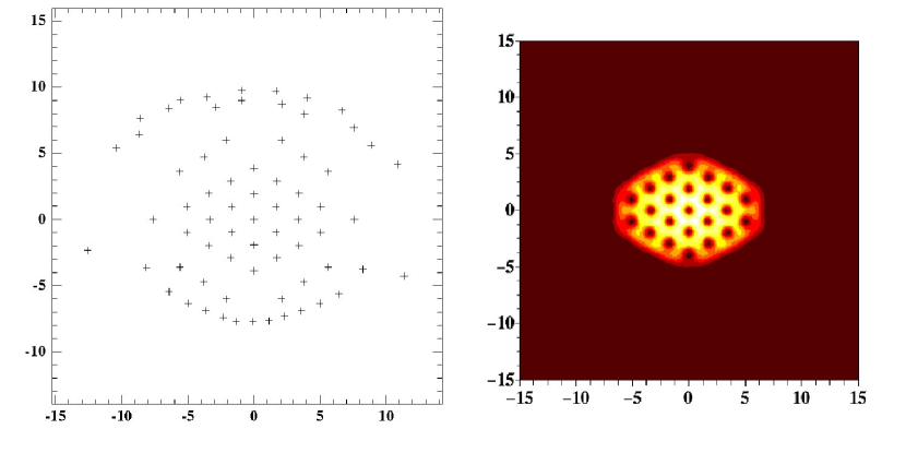
Figure 1. Plot of the zeroes of the minimizer (left) and the density (right) for $\varepsilon^{2}=0.002$, $\nu=0.03$. Triangular vortex lattice in an anisotropic trap.

$\bullet$ $\nu\gg\varepsilon^{1/3}$ (strong anisotropy): $R_{2}\to 0$ (in fact $R_{2}^{4/3}\approx\varepsilon^{1/3}\nu^{-1}$). Numerical simulations (Figure 2) show that there are no vortices in the bulk, the behaviour is an inverted parabola in the $x_{1}$ direction and a fixed Gaussian in the $x_{2}$ direction. Thus, the size of the condensate does not shrink in the $x_{2}$ direction and (1.25) is not a good approximation of the minimizer. The shrinking of the condensate in the $x_{2}$ direction is not allowed in $\Lambda_{0}$ (see (1.22)) because the operator $x_{2}^{2}$ is bounded from below in that space by a positive constant and the first eigenfunction is a Gaussian in the $x_{2}$ direction. We find an asymptotic 1D problem (upper and lower bounds match) which yields a separation of variables.

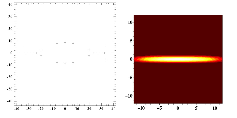
Figure 2. Plot of the zeroes of the minimizer (left) and the density (right) for $\varepsilon^{2}=0.002$, $\nu=0.73$. No vortex in the visible region.

1.4. Main results

1.4.1. Weakly anisotropic case

In a first step, we assume that, with $\kappa$ given by (1.20),

(1.26) $${\varepsilon\leq\kappa\ll\varepsilon^{1/3}}.$$

The isotropic case is recovered by assuming $\kappa=\varepsilon.$ This case is similar to the isotropic case and we derive similar results to the paper [3], namely an upper bound given by the Theta function but we lack a good lower bound.

We recall that the Jacobi Theta function $\Theta(z,\tau)$ associated to a lattice $\mathbb{Z}\oplus\mathbb{Z}\tau$ is a holomorphic function which vanishes exactly once in any lattice cell and is defined by

(1.27) $$\Theta(z,\tau)=\frac{1}{i}\sum_{n=-\infty}^{+\infty}(-1)^{n}e^{i\pi\tau(n+1/2)^{2}}e^{(2n+1)\pi iz},\quad z\in\mathbb{C}\,.$$

This function allows us to construct a periodic function on the same lattice: $u_{\tau}$ is defined by

(1.28) $$u_{\tau}(x_{1},x_{2})=e^{\frac{\pi}{2}\left(z^{2}-|z|^{2}\right)}\Theta\left(\sqrt{\tau_{I}}z,\tau\right),\quad z=x_{1}+ix_{2},\quad\tau=\tau_{R}+i\tau_{I},$$

$|u_{\tau}|$ is periodic over the lattice $\mathbb{Z}\oplus\tau\mathbb{Z}$, and $u_{\tau}$ satisfies

(1.29) $$\Pi_{0}\left(|u_{\tau}|^{2}u_{\tau}\right)=\lambda_{\tau}u_{\tau},$$

with

(1.30) $$\lambda_{\tau}=\frac{\mathchoice{{\vbox{\hbox{$\textstyle-$}}\kern-4.86108pt}}{{\vbox{\hbox{$\scriptstyle-$}}\kern-3.25pt}}{{\vbox{\hbox{$\scriptscriptstyle-$}}\kern-2.29166pt}}{{\vbox{\hbox{$\scriptscriptstyle-$}}\kern-1.875pt}}\!\int|u_{\tau}|^{4}}{\mathchoice{{\vbox{\hbox{$\textstyle-$}}\kern-4.86108pt}}{{\vbox{\hbox{$\scriptstyle-$}}\kern-3.25pt}}{{\vbox{\hbox{$\scriptscriptstyle-$}}\kern-2.29166pt}}{{\vbox{\hbox{$\scriptscriptstyle-$}}\kern-1.875pt}}\!\int|u_{\tau}|^{2}}=\frac{\gamma(\tau)}{\sqrt{2\tau_{I}}},$$

and

(1.31) $$\gamma(\tau):=\frac{\mathchoice{{\vbox{\hbox{$\textstyle-$}}\kern-4.86108pt}}{{\vbox{\hbox{$\scriptstyle-$}}\kern-3.25pt}}{{\vbox{\hbox{$\scriptscriptstyle-$}}\kern-2.29166pt}}{{\vbox{\hbox{$\scriptscriptstyle-$}}\kern-1.875pt}}\!\int|u_{\tau}|^{4}}{\left(\mathchoice{{\vbox{\hbox{$\textstyle-$}}\kern-4.86108pt}}{{\vbox{\hbox{$\scriptstyle-$}}\kern-3.25pt}}{{\vbox{\hbox{$\scriptscriptstyle-$}}\kern-2.29166pt}}{{\vbox{\hbox{$\scriptscriptstyle-$}}\kern-1.875pt}}\!\int|u_{\tau}|^{2}\right)^{2}}.$$

The minimization of $\gamma(\tau)$ on all possible $\tau$ corresponds to the Abrikosov problem. It turns out that the properties of the Theta function allow to derive that

$$\gamma(\tau)=\sum_{(j,k)\in\mathbb{Z}^{2}}e^{-\frac{\pi}{\tau_{I}}|j\tau-k|^{2}}$$

and prove (see [3]) that $\tau\mapsto\gamma(\tau)$ is minimized for $\tau=j=e^{2i\pi/3}$, which corresponds to the hexagonal lattice. The minimum is

(1.32) $$b=\gamma(j)\approx 1.1596.$$

The function $u_{\tau}$ allows us to construct the vortex lattice and we multiply it by the proper inverted parabola to get a good upper bound:

Theorem 1.1.

We have for $I(\varepsilon,\kappa)$ defined in (1.24), $b$ given in (1.32), $\kappa$ in (1.20),

(1.33) $$\frac{2}{3}\sqrt{\frac{2g_{0}\varepsilon\kappa}{\pi}}<I(\varepsilon,\kappa)\leq\frac{2}{3}\sqrt{\frac{2g_{0}b\varepsilon\kappa}{\pi}}+O\left(\sqrt{\varepsilon\kappa}\left(\frac{\kappa^{3}}{\varepsilon}\right)^{1/8}\right),$$

when $(\epsilon,\kappa\epsilon^{-1/3})\to(0,0)$. Moreover, the following function provides the upper bound:

(1.34) $$v=\Pi_{0}\left(u_{\tau}\rho\right),$$

where $u_{\tau}$ is defined by $(\ref{eq:utau})$ with $\tau=e^{\frac{2i\pi}{3}}$ and

$$\rho(x)^{2}=\frac{2}{\pi\sqrt{b}R_{1}R_{2}}\left(1-\frac{x_{1}^{2}}{\sqrt{b}R_{1}^{2}}-\frac{x_{2}^{2}}{\sqrt{b}R_{2}^{2}}\right)_{+},\quad R_{1}=\left(\frac{4g_{0}\kappa}{\pi\varepsilon^{3}}\right)^{1/4},\ R_{2}=\left(\frac{4g_{0}\varepsilon}{\pi\kappa^{3}}\right)^{1/4}.$$

We expect $v$ to be a good approximation of the minimizer and the energy asymptotics to match the right-hand side of (1.33). Thus, the lower bound is not optimal ( it does not include $b$). In addition, the test function (1.34) (with a general $\tau\neq j$ a priori) gives the upper bound of (1.33) with $\gamma(\tau)$ instead of $b$. The proof is a refinement of that in [3].

1.4.2. Strong anisotropy

In the case where the rotation is fast enough in the sense that

(1.35) $${\kappa\gg\varepsilon^{1/3}}$$

we have found a regime unknown by physicists where vortices disappear and the problem can be reduced in fact to a 1D energy.

Theorem 1.2.

For $I(\varepsilon,\kappa)$ defined in (1.24), $b$ given in (1.32), $\kappa$ in (1.20), we have

(1.36) $$\lim_{(\epsilon,\epsilon^{1/3}\kappa^{-1})\to(0,0)}\left(\frac{I(\varepsilon,\kappa)-\frac{\kappa^{2}}{8\pi}}{\varepsilon^{2/3}}\right)=J,$$

where

(1.37) $$J=\inf\bigl{\{}\int\frac{1}{2}t^{2}p(t)^{2}+\frac{g_{0}}{2}\int p(t)^{4},\ p\text{ real-valued }\in L^{2}(\mathbb{R})\cap L^{4}(\mathbb{R}),\|p\|_{L^{2}(\mathbb{R})}=1\bigr{\}}.$$

In addition, if $u$ is a minimizer of $I(\varepsilon,\kappa)$, then

(1.38) $$\frac{1}{\varepsilon^{1/3}}\left|u\left(\frac{x_{1}}{\varepsilon^{2/3}},x_{2}\right)\right|\longrightarrow 2^{1/4}e^{-\pi x_{2}^{2}}p(x_{1}),$$

in $L^{2}(\mathbb{R}^{2})\cap L^{4}(\mathbb{R}^{2})$, where $p$ is the minimizer of $J.$

Note that the minimizer $p$ of (1.37) is explicit:

$$p(t)^{2}=\frac{3}{4R}\left(1-\frac{t^{2}}{R^{2}}\right)_{+},\quad R=\left(\frac{3g_{0}}{2}\right)^{1/3}.$$

A few words about the proof of Theorem 1.2. The first point is that the operator $\Pi_{0}x_{2}^{2}\Pi_{0}$ (see (1.22), (1.23)) is bounded from below by a positive constant:

$$\forall u\in\Lambda_{0},\quad\int_{\mathbb{R}^{2}}x_{2}^{2}|u|^{2}\geq\frac{1}{4\pi}\int_{\mathbb{R}^{2}}|u|^{2}.$$

This is proven in Lemma 4.4 below. Actually, the spectrum of this operator is purely continuous, and any Weyl sequence associated with the value $1/(4\pi)$ converges (up to renormalization) to the function

(1.39) $$u_{0}(x_{1},x_{2})=\exp\left(-\pi x_{2}^{2}+i\pi x_{1}x_{2}\right),$$

which satisfies the equation $\Pi_{0}(u_{0})=\frac{1}{4\pi}u_{0}.$ This gives the lower bound

$$I(\varepsilon,\kappa)\geq\frac{\kappa^{2}}{8\pi},$$

and indicates that in order to be close to this lower bound, a test function should be close to (1.39). Thus, the second point is to construct a test function having the same behaviour as (1.39) in $x_{2}$, and a large extension in $x_{1}$. This is done by using the function

$$u_{1}(x_{1},x_{2})=\frac{1}{2^{1/4}}e^{-\frac{\pi}{2}x_{2}^{2}}\int_{\mathbb{R}}e^{-\frac{\pi}{2}\left((x_{1}-y_{1})^{2}-2iy_{1}x_{2}\right)}\rho(y_{1})dy_{1},$$

which is equal to $\Pi_{0}(\rho(x_{1})\delta_{0}(x_{2}))$, where $\delta_{0}$ is the Dirac delta function and $\rho$ any real-valued function of one variable. This test function is then proved to be close to $2^{1/4}e^{-\pi x_{2}^{2}}\rho(x_{1}),$ which allows to compute its energy, and gives the upper bound, provided that $\rho(t)=\varepsilon^{1/3}p(\varepsilon^{2/3}t)$, where $p$ is the minimizer of (1.37). Finally, in order to prove the lower bound, we first extract bounds on the minimizer from the energy, which allow to pass to the limit in the equation (after rescaling as in (1.38)), hence prove that the limit is the right-hand side of (1.38). This uses the fact that the energy appearing in (1.37) is strictly convex, hence that any critical point is the unique minimizer.

The paper is organized as follows: in section 2, we review some standard facts on positive definite quadratic forms in a symplectic space. This allows us, in section 3, to construct a symplectic mapping $\chi$, which yields a simplification of the quadratic form $q$. In section 4, quantizing that symplectic mapping in a metaplectic transformation, we find the expression of the $LLL$ and manage to reach the reduced form of the energy (Proposition 4.5). Section 5 is devoted to the proof of Theorem 1.1 and section 6 to Theorem 1.2.

Open questions

We have no information on the the intermediate regime where, for instance, $\varepsilon^{1/3}/\kappa$ converges to some constant $R_{0}^{4/3}$ (in that case, $R_{1}\approx\varepsilon^{-2/3},R_{2}\approx R_{0}$). We expect that the extension in the $x_{2}$ direction depends on $R_{0}$ and wonder whether the condensate has a finite number of vortex lines. We have not determined the limiting problem. Acknowledgements. We would like to thank A.L.Fetter and J.Dalibard for very useful comments on the physics of the problem. We also acknowledge support from the French ministry grant ANR-BLAN-0238, VoLQuan and express our gratitude to our colleagues participating to this ANR-project, in particular T.Jolicœur and S.Ouvry.

2. Quadratic Hamiltonians

We first review some standard facts on positive definite quadratic forms in a symplectic space.

2.1. On positive definite quadratic forms on symplectic spaces

We consider the phase space $\mathbb{R}^{n}_{x}\times\mathbb{R}^{n}_{\xi}$, equipped with its canonical symplectic structure: the symplectic form $\sigma$ is a bilinear alternate form on $\mathbb{R}^{2n}$ given by

(2.1) $$\sigma\bigl{(}(x,\xi);(y,\eta)\bigr{)}=\xi\cdot y-\eta\cdot x=\langle\sigma X,Y\rangle,$$

(2.2) $$\text{with\quad}{X=\begin{pmatrix}x\\ \xi\end{pmatrix},Y=\begin{pmatrix}y\\ \eta\end{pmatrix},\sigma=\begin{pmatrix}0&I_{n}\\ -I_{n}&0\end{pmatrix},}$$

where the form $\sigma$ is identified with the $2n\times 2n$ matrix above given in $n\times n$ blocks. The symplectic group $Sp(n)$ (a subgroup of $Sl(2n,\mathbb{R})$), is defined by the equation on the $2n\times 2n$ matrix $\chi$,

(2.3) $$\chi^{*}\sigma\chi=\sigma,\quad\text{ i.e. $\forall X,Y\in\mathbb{R}^{2n},\ \langle\sigma\chi X,\chi Y\rangle=\langle\sigma X,Y\rangle$}.$$

The following lemma is classical (see e.g. the chapter XXI in [10], or [15]).

Lemma 2.1.

Let $B\in GL(n,\mathbb{R})$ and let $A,C$ be $n\times n$ real symmetric matrices.  Then the matrix $\Xi$, given by $n\times n$ blocks

(2.4) $$\Xi_{A,B,C}=\begin{pmatrix}B^{-1}&-B^{-1}C\\ AB^{-1}&B^{*}-AB^{-1}C\end{pmatrix}=\begin{pmatrix}I&0\\ A&I\end{pmatrix}\begin{pmatrix}B^{-1}&0\\ 0&B^{*}\end{pmatrix}\begin{pmatrix}I&-C\\ 0&I\end{pmatrix}$$

belongs to $Sp(n)$. Any element of $Sp(n)$ can be written as a product

$$\Xi_{A_{1},B_{1},C_{1}}\Xi_{A_{2},B_{2},C_{2}}.$$

N.B.

The first statement is easy to verify directly and we shall not use the last statement, which is nevertheless an interesting piece of information. For a symplectic mapping $\Xi$, to be of the form above is equivalent to the assumption that the mapping $x\mapsto pr_{1}\Xi(x\oplus 0)$ is invertible from $\mathbb{R}^{n}$ to $\mathbb{R}^{n}$.

Given a quadratic form $Q$ on $\mathbb{R}^{2n}$, identified with a symmetric $2n\times 2n$ matrix, we define its fundamental matrix $F$ by the identity

$$F=-\sigma^{-1}Q=\sigma Q,\quad\text{so that for $X,Y\in\mathbb{R}^{2n}$ }\quad\langle\sigma Y,FX\rangle=\langle QY,X\rangle.$$

The following proposition is classical (see e.g. the theorem 21.5.3 in [10]).

Proposition 2.2.

Let $Q$ be a positive definite quadratic form on the symplectic $\mathbb{R}^{n}_{x}\times\mathbb{R}^{n}_{\xi}$. One can find $\chi\in Sp(n)$ such that with

$$\mathbb{R}^{2n}\ni X=\chi Y,\quad Y=(y_{1},\dots,y_{n},\eta_{1},\dots,\eta_{n}),$$

$$\langle QX,X\rangle=\langle Q\chi Y,\chi Y\rangle=\sum_{1\leq j\leq n}(\eta_{j}^{2}+\mu_{j}^{2}y_{j}^{2}),\quad\mu_{j}>0.$$

The $\{\pm i\mu_{j}\}_{1\leq j\leq n}$ are the $2n$ eigenvalues of the fundamental matrix, related to the $2n$ eigenvectors $\{e_{j}\pm i\varepsilon_{j}\}_{1\leq j\leq n}.$ The $\{e_{j},\varepsilon_{j}\}_{1\leq j\leq n}$ make a symplectic basis of $\mathbb{R}^{2n}$:

$$\sigma(\varepsilon_{j},e_{k})=\delta_{j,k},\quad\sigma(\varepsilon_{j},\varepsilon_{k})=\sigma(e_{j},e_{k})=0,$$

and the symplectic planes $\Pi_{j}=\mathbb{R}e_{j}\oplus\mathbb{R}\varepsilon_{j}$ are orthogonal for $Q$.

N.B.

A one-line-proof of these classical facts: on $\mathbb{C}^{2n}$ equipped with the dot-product given by $Q$, diagonalize the sesquilinear Hermitian form $i\sigma$.

2.2. Generating functions

We define on $\mathbb{R}^{n}\times\mathbb{R}^{n}$ the generating function $S$ of the symplectic mapping of the form $\Xi_{A,B,C}$ given in the lemma 2.1 by the identity

(2.5) $$S(x,\eta)=\frac{1}{2}\bigl{(}\langle Ax,x\rangle+2\langle Bx,\eta\rangle+\langle C\eta,\eta\rangle\bigr{)}.$$

We have

(2.6) $$\Xi_{A,B,C}\underbrace{\Bigl{(}\frac{\partial S}{\partial\eta},\eta\Bigr{)}}_{\in\mathbb{R}^{n}\times\mathbb{R}^{n}}=\underbrace{\Bigl{(}x,\frac{\partial S}{\partial x}\Bigr{)}}_{\in\mathbb{R}^{n}\times\mathbb{R}^{n}}.$$

In fact, we see directly

$$\begin{pmatrix}I&0\\ A&I\end{pmatrix}\begin{pmatrix}B^{-1}&0\\ 0&B^{*}\end{pmatrix}\begin{pmatrix}I&-C\\ 0&I\end{pmatrix}\begin{pmatrix}Bx+C\eta\\ \eta\end{pmatrix}=\begin{pmatrix}I&0\\ A&I\end{pmatrix}\begin{pmatrix}x\\ B^{*}\eta\end{pmatrix}=\begin{pmatrix}x\\ Ax+B^{*}\eta\end{pmatrix}.$$

Given a positive definite quadratic form $Q$ on $\mathbb{R}^{2n}$, identified with a symmetric $2n\times 2n$ matrix, we know from the proposition 2.2 that there exists $\chi\in Sp(n)$ such that

$$\chi^{*}Q\chi=\begin{pmatrix}\mu^{2}&0\\ 0&I_{n}\end{pmatrix},\quad\mu^{2}=\operatorname{diag}(\mu_{1}^{2},\dots,\mu_{n}^{2})$$

Looking for $\chi=\Xi_{A,B,C}$ given by a generating function $S$ as above, we end-up (using the notation $q(X)=\langle QX,X\rangle$ with $X\in\mathbb{R}^{2n}$) with the equation

$$q(\underbrace{x,\partial_{x}S}_{\mathbb{R}^{n}\times\mathbb{R}^{n}})=\|\mu\partial_{\eta}S\|^{2}+\|\eta\|^{2},\qquad\mu\partial_{\eta}S=(\mu_{j}\partial_{\eta_{j}}S)_{1\leq j\leq n}\in\mathbb{R}^{n},$$

where $\|\cdot\|$ stands for the standard Euclidean norm on $\mathbb{R}^{n}$. This means

(2.7) $$q(x,Ax+B^{*}\eta)=\|\mu(Bx+C\eta)\|^{2}+\|\eta\|^{2}.$$

We want now to go back to the study of our quadratic form (1.12).

2.3. Effective diagonalization

Lemma 2.3.

Let $q$ be the quadratic form on $\mathbb{R}^{4}$ given by (1.12), where $\omega,\nu,\varepsilon$ are nonnegative parameters such that $\omega^{2}+\nu^{2}+\varepsilon^{2}=1$. The eigenvalues of the fundamental matrix are $\pm i\mu_{1},\pm i\mu_{2}$ with

(2.8) $$0 \leq\mu_{1}^{2}=1+\omega^{2}-\alpha\leq\mu_{2}^{2}=1+\omega^{2}+\alpha,\quad\alpha=\sqrt{\nu^{4}+4\omega^{2}},$$

(2.9) $$\mu_{1}^{2} =\frac{2\nu^{2}\varepsilon^{2}+\varepsilon^{4}}{\mu_{2}^{2}}.$$

In the isotropic case $\nu=0$, we recover $\mu_{1}=1-\omega,\mu_{2}=1+\omega.$ When $\varepsilon>0$, we have $0<\mu_{1}^{2}\leq\mu_{2}^{2}$ and $q$ is positive-definite. When $\varepsilon=0$, we have $\mu_{1}=0<\mu_{2}$, and $q$ is positive semi-definite with rank $2$ if $\nu=0$ and with rank $3$ if $\nu>0$.

Proof.

The matrix $Q$ of $q$ is thus

(2.10) $${Q=\begin{pmatrix}1-\nu^{2}&0&0&-\omega\\ 0&1+\nu^{2}&\omega&0\\ 0&\omega&1&0\\ -\omega&0&0&1\end{pmatrix}},\text{\ and }F=\sigma Q=\begin{pmatrix}0&\omega&1&0\\ -\omega&0&0&1\\ \nu^{2}-1&0&0&\omega\\ 0&-\nu^{2}-1&-\omega&0\end{pmatrix}.$$

The characteristic polynomial $p$ of $F$ is easily seen to be even and we calculate

$$p(\lambda)=\det(F-\lambda I_{4})=\lambda^{4}+2(1+\omega^{2})\lambda^{2}+(1-\omega^{2})^{2}-\nu^{4}=(\lambda^{2}+1+\omega^{2})^{2}-(\nu^{4}+4\omega^{2}).$$

The four eigenvalues of $F$ are thus $\pm i\sqrt{1+\omega^{2}\pm\sqrt{\nu^{4}+4\omega^{2}}},$ proving the first statement of the lemma. Since $(1+\omega^{2})^{2}-\alpha^{2}=(1-\omega^{2})^{2}-\nu^{4}=\varepsilon^{2}(2\nu^{2}+\varepsilon^{2})$, we get $\mu_{1}^{2}={\varepsilon^{2}(2\nu^{2}+\varepsilon^{2})}/{\mu_{2}^{2}}.$ The statements on the cases $\nu=0,\varepsilon>0$ are now obvious. When $\varepsilon=0=\nu$, we have $\omega=1$, and $\operatorname{rank}q=2$ as it is obvious on (1.17). When $\varepsilon=0,\nu>0$, we consider the following minor determinant in $F$, cofactor of $f_{31}$

$$\left|\begin{matrix}\omega&1&0\ \\ 0&0&1\ \\ -\nu^{2}-1&-\omega&0\ \end{matrix}\right|=(-1)(-\omega^{2}+\nu^{2}+1)=-2\nu^{2}\not=0,$$

so that $\operatorname{rank}Q=\operatorname{rank}F=3$ in that case. ∎

N.B.

We may note here that the condition $\omega^{2}+\nu^{2}\leq 1$ is an iff condition on the real parameters $\nu,\omega$ for the quadratic form (1.12) to be positive semi-definite. This is obvious on the expression (1.17) in the isotropic case $\nu=0$, and more generally, the (non-symplectic) decomposition in independent linear forms

$$q=(\xi_{1}+\omega x_{2})^{2}+(\xi_{2}-\omega x_{1})^{2}+x_{1}^{2}(1-\nu^{2}-\omega^{2})+x_{2}^{2}(1+\nu^{2}-\omega^{2}),$$

shows that $q$ has exactly one negative eigenvalue when $\omega^{2}+\nu^{2}>1\geq\omega^{2}-\nu^{2}$, and exactly two negative eigenvalues when $\omega^{2}-\nu^{2}>1$. As a result, when $\omega^{2}+\nu^{2}>1$, the operator $q^{w}$ is unbounded from below.

Using now the equations (2.7), (1.12) and assuming that we may find a linear symplectic transformation given by a generating function (2.5), we have to find $A,B,C$ like in the lemma 2.1 with $n=2$, so that for all $(x,\eta)\in\mathbb{R}^{2}\times\mathbb{R}^{2}$,

$$\|Ax+B^{*}\eta\|^{2}+\|x\|^{2}+\nu^{2}(x_{2}^{2}-x_{1}^{2})-2\omega\bigl{(}x\wedge(Ax+B^{*}\eta)\bigr{)}=\|\mu(Bx+C\eta)\|^{2}+\|\eta\|^{2},$$

with $x\wedge\xi=x_{1}\xi_{2}-x_{2}\xi_{1},\mu=\operatorname{diag}({\mu_{1},\mu_{2}}).$ At this point, we see that the previous identity forces some relationships between the matrices $A,B,C$. However, the algebra is somewhat complicated and assuming that $B$ is diagonal, $A,C$ are (symmetrical) with zeroes on the diagonal lead to some simplifications and to the following results. We introduce first some parameters:

(2.11) $$\beta_{1} =\frac{2\omega\mu_{1}}{\alpha-2\omega^{2}+\nu^{2}}=\frac{\alpha-2\omega^{2}-\nu^{2}}{2\omega\mu_{1}}\ \text{\tiny since $(\alpha-2\omega^{2})^{2}-\nu^{4}=4\omega^{2}+4\omega^{4}-4\omega^{2}\alpha=4\omega^{2}\mu_{1}^{2}$ },$$

(2.12) $$\beta_{2} =\frac{2\omega\mu_{2}}{\alpha+2\omega^{2}+\nu^{2}}=\frac{\alpha+2\omega^{2}-\nu^{2}}{2\omega\mu_{2}}\ \text{\tiny since $(\alpha+2\omega^{2})^{2}-\nu^{4}=4\omega^{2}+4\omega^{4}+4\omega^{2}\alpha=4\omega^{2}\mu_{2}^{2}$ },$$

(2.13) $$\gamma=\frac{2\alpha}{\omega},$$

(2.14) $$\lambda_{1}^{2}=\frac{\mu_{1}}{\mu_{1}+\beta_{1}\beta_{2}\mu_{2}}=\frac{1}{1+\frac{\beta_{1}\beta_{2}\mu_{2}}{\mu_{1}}}=\frac{1}{1+\frac{\alpha+2\omega^{2}-\nu^{2}}{\alpha-2\omega^{2}+\nu^{2}}}=\frac{\alpha-2\omega^{2}+\nu^{2}}{2\alpha},$$

(2.15) $$\lambda_{2}^{2}=\frac{\mu_{2}}{\mu_{2}+\beta_{1}\beta_{2}\mu_{1}}=\frac{1}{1+\frac{\beta_{1}\beta_{2}\mu_{1}}{\mu_{2}}}=\frac{1}{1+\frac{\alpha-2\omega^{2}-\nu^{2}}{\alpha+2\omega^{2}+\nu^{2}}}=\frac{\alpha+2\omega^{2}+\nu^{2}}{2\alpha},$$

and we have

(2.16) $$\lambda_{1}^{2}+\lambda_{2}^{2}=1+\frac{\nu^{2}}{\alpha},\qquad\lambda_{1}^{2}\lambda_{2}^{2}=\frac{(\alpha+\nu^{2})^{2}-4\omega^{4}}{4\alpha^{2}}.$$

We define also

(2.17) $$d=\frac{\gamma\lambda_{1}\lambda_{2}}{2},\quad c=\frac{\lambda_{1}^{2}+\lambda_{2}^{2}}{2\lambda_{1}\lambda_{2}}\quad\text{ \footnotesize which gives }\quad cd=\frac{2\alpha(1+\nu^{2}/\alpha)}{4\omega}=\frac{\alpha+\nu^{2}}{2\omega}.$$

Lemma 2.4.

We define the $2\times 2$ matrices

$$B=\begin{pmatrix}\lambda_{1}^{-1}&0\\ 0&\lambda_{2}^{-1}\end{pmatrix},\quad C=\begin{pmatrix}0&d^{-1}\\ d^{-1}&0\end{pmatrix},\quad A=\begin{pmatrix}0&\frac{d}{\lambda_{1}\lambda_{2}}-cd\\ \frac{d}{\lambda_{1}\lambda_{2}}-cd&0\end{pmatrix}.$$

The $4\times 4$ matrix given with $2\times 2$ blocks by

$$\chi=\Xi_{A,B,C}=\begin{pmatrix}I_{2}&0\\ A&I_{2}\end{pmatrix}\begin{pmatrix}B^{-1}&0\\ 0&B^{*}\end{pmatrix}\begin{pmatrix}I_{2}&-C\\ 0&I_{2}\end{pmatrix}$$

belongs to $Sp(2)$ and

(2.18) $$\chi=\begin{pmatrix}\lambda_{1}&0&0&-\frac{\lambda_{1}}{d}\\ 0&\lambda_{2}&-\frac{\lambda_{2}}{d}&0\\ 0&\frac{d}{\lambda_{1}}-\lambda_{2}cd&c\lambda_{2}&0\\ \frac{d}{\lambda_{2}}-\lambda_{1}cd&0&0&c\lambda_{1}\end{pmatrix},$$

(2.19) $$\chi^{-1}=\begin{pmatrix}c\lambda_{2}&0&0&\frac{\lambda_{2}}{d}\\ 0&c\lambda_{1}&\frac{\lambda_{1}}{d}&0\\ 0&-\frac{d}{\lambda_{2}}+\lambda_{1}cd&\lambda_{1}&0\\ -\frac{d}{\lambda_{1}}+\lambda_{2}cd&0&0&\lambda_{2}\end{pmatrix}.$$

Proof.

The lemma 2.1 gives that $\chi\in Sp(2)$ and we have also

$$\chi^{-1}=\begin{pmatrix}I_{2}&C\\ 0&I_{2}\end{pmatrix}\begin{pmatrix}B&0\\ 0&{B^{*}}^{-1}\end{pmatrix}\begin{pmatrix}I_{2}&0\\ -A&I_{2}\end{pmatrix}.$$

The remaining part of the proof depends on the formula giving $\Xi_{A,B,C}$ in the lemma 2.1 and a direct computation whose verification is left to the reader. ∎

Lemma 2.5.

Let $\chi$ be the symplectic matrix given by (2.18) and $Q$ be the matrix given in (2.10). Then, with $\mu_{j}$ given by (2.8), we have

(2.20) $$\chi^{*}Q\chi=\operatorname{diag}(\mu_{1}^{2},\mu_{2}^{2},1,1).$$

The (tedious) proof of that lemma is given in the appendix 7.3.1.

Using the expression of $\chi^{-1}$ in (2.18), defining

(2.21) $$\begin{pmatrix}y_{1}\\ y_{2}\\ \eta_{1}\\ \eta_{2}\end{pmatrix}=\begin{pmatrix}c\lambda_{2}&0&0&\frac{\lambda_{2}}{d}\\ 0&c\lambda_{1}&\frac{\lambda_{1}}{d}&0\\ 0&-\frac{d}{\lambda_{2}}+\lambda_{1}cd&\lambda_{1}&0\\ -\frac{d}{\lambda_{1}}+\lambda_{2}cd&0&0&\lambda_{2}\end{pmatrix}\begin{pmatrix}x_{1}\\ x_{2}\\ \xi_{1}\\ \xi_{2}\end{pmatrix},$$

we get from the lemma 2.5 the following result.

Lemma 2.6.

For $(x_{1},x_{2},\xi_{1},\xi_{2})\in\mathbb{R}^{4}$, $(y_{1},y_{2},\eta_{1},\eta_{2})\in\mathbb{R}^{4}$ given by (2.21), we have the following identity,

$$\mu_{1}^{2}y_{1}^{2}+\mu_{2}^{2}y_{2}^{2}+\eta_{1}^{2}+\eta_{2}^{2} =\mu_{1}^{2}\bigl{(}c\lambda_{1}x_{2}+\lambda_{2}d^{-1}\xi_{2}\bigr{)}^{2}+\mu_{2}^{2}\bigl{(}c\lambda_{2}x_{1}+\lambda_{1}d^{-1}\xi_{1}\bigr{)}^{2}$$

$${\hskip 15.0pt}+\bigl{(}(-d\lambda_{2}^{-1}+\lambda_{1}cd)x_{2}+\lambda_{1}\xi_{1}\bigr{)}^{2}+\bigl{(}(-d\lambda_{1}^{-1}+\lambda_{2}cd)x_{1}+\lambda_{2}\xi_{2}\bigr{)}^{2}$$

$$=\xi_{1}^{2}+\xi_{2}^{2}+(1-\nu^{2})x_{1}^{2}+(1+\nu^{2})x_{2}^{2}-2\omega(x_{1}\xi_{2}-x_{2}\xi_{1}),$$

where the parameters $c,\lambda_{2},d,\lambda_{1}$ are defined above (note that all these parameters are well-defined when $(\omega,\nu)$ are both positive with $\omega^{2}+\nu^{2}<1$).

We have achieved an explicit diagonalization of the quadratic form (1.12) and, most importantly, that diagonalization is performed via a symplectic mapping. That feature will be of particular importance in our next section. Expressing the parameters in terms of $\alpha,\omega,\nu,\varepsilon$ (cf. section 7.2), we obtain

$$q =\Bigl{(}2^{-1/2}\alpha^{-1/2}(\alpha-2\omega^{2}+\nu^{2})^{1/2}\xi_{1}-2^{-3/2}\omega^{-1}\alpha^{-1/2}(\alpha-2\omega^{2}+\nu^{2})^{1/2}(\alpha-\nu^{2})x_{2}\Bigr{)}^{2}$$

$$+\Bigl{(}2^{-1/2}\alpha^{-1/2}\bigl{(}\frac{\alpha+2\omega^{2}-\nu^{2}}{2\nu^{2}+\varepsilon^{2}}\bigr{)}^{1/2}\frac{(2\nu^{2}\varepsilon^{2}+\varepsilon^{4})^{1/2}}{\mu_{2}}\xi_{2}$$

$$\hskip 84.0pt+\frac{(2\nu^{2}\varepsilon^{2}+\varepsilon^{4})^{1/2}}{\mu_{2}}(\alpha^{1/2}+\nu^{2}\alpha^{-1/2})2^{-3/2}\omega^{-1}\bigl{(}\frac{\alpha+2\omega^{2}-\nu^{2}}{2\nu^{2}+\varepsilon^{2}}\bigr{)}^{1/2}x_{1}\Bigr{)}^{2}$$

$$+\Bigl{(}(1+\omega^{2}+\alpha)^{1/2}2^{1/2}\alpha^{-1/2}\omega(\alpha+2\omega^{2}+\nu^{2})^{-1/2}\xi_{1}$$

$$\hskip 84.0pt+(1+\omega^{2}+\alpha)^{1/2}(1+\alpha^{-1}\nu^{2})2^{-1/2}\alpha^{1/2}(\alpha+2\omega^{2}+\nu^{2})^{-1/2}x_{2}\Bigr{)}^{2}$$

$$+\Bigl{(}2^{-1/2}\alpha^{-1/2}(\alpha+2\omega^{2}+\nu^{2})^{1/2}\xi_{2}-2^{-3/2}\omega^{-1}\alpha^{-1/2}(\alpha-\nu^{2})(\alpha+2\omega^{2}+\nu^{2})^{1/2}x_{1}\Bigr{)}^{2},$$

so that

(2.22) $$\begin{split}q&=\overbrace{\Bigl{(}\frac{\alpha-2\omega^{2}+\nu^{2}}{2\alpha}\Bigr{)}\Bigl{[}\xi_{1}-\bigl{(}\frac{\alpha-\nu^{2}}{2\omega}\bigr{)}x_{2}\Bigr{]}^{2}}^{\eta_{1}^{2}}+\overbrace{\Bigl{(}\frac{\alpha+2\omega^{2}-\nu^{2}}{2\alpha\mu_{2}^{2}}\Bigr{)}\varepsilon^{2}\Bigl{[}\xi_{2}+\bigl{(}\frac{\alpha+\nu^{2}}{2\omega}\bigr{)}x_{1}\Bigr{]}^{2}}^{\mu_{1}^{2}y_{1}^{2}}\\ &+\underbrace{2\omega^{2}\Bigl{(}\frac{1+\omega^{2}+\alpha}{\alpha(\alpha+2\omega^{2}+\nu^{2})}\Bigr{)}\Bigl{[}\xi_{1}+\bigl{(}\frac{\alpha+\nu^{2}}{2\omega}\bigr{)}x_{2}\Bigr{]}^{2}}_{\mu_{2}^{2}y_{2}^{2}}+\underbrace{\Bigl{(}\frac{\alpha+2\omega^{2}+\nu^{2}}{2\alpha}\Bigr{)}\Bigl{[}\xi_{2}-\bigl{(}\frac{\alpha-\nu^{2}}{2\omega}\bigr{)}x_{1}\Bigr{]}^{2}}_{\eta_{2}^{2}}.\end{split}$$

The equation (2.22) encapsulates most of our previous work on the diagonalization of $q$. In the appendix 7.3.2, we provide another way of checking the symplectic relationships between the linear forms, $y_{j},\eta_{l}$.

We have seen in Lemma 2.3 that when $\varepsilon=0,\nu>0$, the rank of $q$ is 3, whereas its symplectic rank is 2. Indeed, $\varepsilon=0$ and $\nu>0$, we have

(2.23) $$\begin{split}q&=\overbrace{\Bigl{(}\frac{\alpha-2\omega^{2}+\nu^{2}}{2\alpha}\Bigr{)}\Bigl{[}\xi_{1}-\bigl{(}\frac{\alpha-\nu^{2}}{2\omega}\bigr{)}x_{2}\Bigr{]}^{2}}^{\eta_{1}^{2}}+\\ &+\underbrace{2\omega^{2}\Bigl{(}\frac{1+\omega^{2}+\alpha}{\alpha(\alpha+2\omega^{2}+\nu^{2})}\Bigr{)}\Bigl{[}\xi_{1}+\bigl{(}\frac{\alpha+\nu^{2}}{2\omega}\bigr{)}x_{2}\Bigr{]}^{2}}_{\mu_{2}^{2}y_{2}^{2}}+\underbrace{\Bigl{(}\frac{\alpha+2\omega^{2}+\nu^{2}}{2\alpha}\Bigr{)}\Bigl{[}\xi_{2}-\bigl{(}\frac{\alpha-\nu^{2}}{2\omega}\bigr{)}x_{1}\Bigr{]}^{2}}_{\eta_{2}^{2}}.\end{split}$$

3. Quantization

3.1. The Irving E. Segal formula

Let $a$ be defined on $\mathbb{R}^{n}_{x}\times\mathbb{R}^{n}_{\xi}$ (say a tempered distribution on $\mathbb{R}^{2n}$). Its Weyl quantization is the operator, acting for instance on $u\in\mathscr{S}(\mathbb{R}^{n})$,

(3.1) $$(a^{w}u)(x)=\iint e^{2i\pi(x-x^{\prime})\xi}a(\frac{x+x^{\prime}}{2},\xi)u(x^{\prime})dx^{\prime}d\xi.$$

In fact, the weak formula $\langle a^{w}u,v\rangle=\int_{\mathbb{R}^{2n}}a(x,\xi)\mathcal{H}(u,v)(x,\xi)dxd\xi$ makes sense for $a\in\mathscr{S}^{\prime}(\mathbb{R}^{2n}),u,v\in\mathscr{S}(\mathbb{R}^{n})$ since the Wigner function $\mathcal{H}(u,v)$ defined by

$$\mathcal{H}(u,v)(x,\xi)=\int e^{-2i\pi x^{\prime}\xi}u(x+\frac{x^{\prime}}{2})\bar{v}(x-\frac{x^{\prime}}{2})dx^{\prime}$$

belongs to $\mathscr{S}(\mathbb{R}^{2n})$ for $u,v\in\mathscr{S}(\mathbb{R}^{n})$ . Note also our definition of the Fourier transform $\hat{u}(\xi)=\int e^{-2i\pi x\cdot\xi}u(x)dx$ (so that $u(x)=\int e^{2i\pi x\cdot\xi}\hat{u}(\xi)d\xi$) and

$$\xi_{j}^{w}u=\frac{1}{2i\pi}\frac{\partial u}{\partial x_{j}}=D_{j}u,\quad x_{j}^{w}u=x_{j}u,\quad(x_{j}\xi_{j})^{w}=\frac{1}{2}\bigl{(}x_{j}D_{j}+D_{j}x_{j}\bigr{)}.$$

Let $\chi$ be a linear symplectic transformation $\chi(y,\eta)=(x,\xi)$. The Segal formula (see e.g. the theorem 18.5.9 in [10]) asserts that there exists a unitary transformation $M$ of $L^{2}(\mathbb{R}^{n})$, uniquely determined apart from a constant factor of modulus one, which is also an automorphism of $\mathscr{S}(\mathbb{R}^{n})$ and $\mathscr{S}^{\prime}(\mathbb{R}^{n})$ such that, for all $a\in\mathscr{S}^{\prime}(\mathbb{R}^{2n})$,

(3.2) $$(a\circ\chi)^{w}=M^{*}a^{w}M,$$

providing the following commutative diagrams

$$\begin{CD}\mathscr{S}(\mathbb{R}^{n}_{x})@>{a^{w}}>{}>\mathscr{S}^{\prime}(\mathbb{R}^{n}_{x})\\ @A{M}A{}A@V{}V{M^{*}}V\\ \mathscr{S}(\mathbb{R}^{n}_{y})@>{}>{(a\circ\chi)^{w}}>\mathscr{S}^{\prime}(\mathbb{R}^{n}_{y})\end{CD}{\hskip 15.0pt}\text{\small and if $a^{w}\in\mathcal{L}(L^{2}(\mathbb{R}^{n}))$}{\hskip 15.0pt}\begin{CD}L^{2}(\mathbb{R}^{n}_{x})@>{a^{w}}>{}>L^{2}(\mathbb{R}^{n}_{x})\\ @A{M}A{}A@V{}V{M^{*}}V\\ L^{2}(\mathbb{R}^{n}_{y})@>{}>{(a\circ\chi)^{w}}>L^{2}(\mathbb{R}^{n}_{y})\end{CD}$$

3.2. The metaplectic group and the generating functions

For a given $\chi$, how can we determine $M$ ? We shall not need here the rich algebraic structure of the two-fold covering $Mp(n)$ (the metaplectic group in which live the transformations $M$) of the symplectic group $Sp(n)$. The following lemma is classical (and also easy to prove directly using the factorization of the lemma 2.1) and provides a simple expression for $M$ when the transformation $\chi$ has a generating function.

Lemma 3.1.

Let $\chi=\Xi_{A,B,C}$ be the symplectic mapping given by (2.4). Then the Segal formula (3.2) holds with

(3.3) $$(Mv)(x)=\int e^{2i\pi S(x,\eta)}\widehat{v}(\eta)d\eta|\det B|^{1/2},$$

where $S$ is given by (2.5).

3.3. Explicit expression for $M$

Lemma 3.2.

Let $\chi$ be the symplectic transformation of $\mathbb{R}^{4}$ given by (2.18). Then the Segal formula (3.2) holds with $M$ given by

(3.4) $$(Mv)(x_{1},x_{2})=(\lambda_{1}\lambda_{2})^{-1/2}e^{2i\pi d\left((\lambda_{1}\lambda_{2})^{-1}-c\right)x_{1}x_{2}}\\ \times\iint e^{2i\pi d^{-1}\eta_{1}\eta_{2}}\widehat{v}(\eta_{1},\eta_{2})e^{2i\pi(\lambda_{1}^{-1}x_{1}\eta_{1}+\lambda_{2}^{-1}x_{2}\eta_{2})}d\eta_{1}d\eta_{2},$$

(3.5) $$(Mv)(x_{1},x_{2})=(\lambda_{1}\lambda_{2})^{-1/2}e^{2i\pi d\left((\lambda_{1}\lambda_{2})^{-1}-c\right)x_{1}x_{2}}(e^{2i\pi d^{-1}D_{1}D_{2}}v)(\lambda_{1}^{-1}x_{1},\lambda_{2}^{-1}x_{2}).$$

Proof.

We apply the lemmas 3.1 and 2.4, along with the fact that the mapping $Mp(n)\ni M\mapsto\chi\in Sp(n)$ is an homomorphism or more elementarily that (3.2) implies for $\chi_{j}\in Sp(n)$,

$$(a\circ\chi_{2}\circ\chi_{1})^{w}=M_{1}^{*}(a\circ\chi_{2})^{w}M_{1}=M_{1}^{*}M_{2}^{*}a^{w}M_{2}M_{1}.$$

The factorization of the lemma 2.4 implies that

$$(Mv)(x)=e^{i\pi\langle Ax,x\rangle}\int_{\mathbb{R}^{2}}e^{2i\pi\langle Bx,\eta\rangle}e^{i\pi\langle C\eta,\eta\rangle}\widehat{v}(\eta)d\eta,$$

which gives readily the formulas above. ∎

Summing-up, we have proven the following result.

Theorem 3.3.

Let $q$ be the quadratic form on $\mathbb{R}^{4}$ given by (1.12). We define the symplectic mapping $\chi$ by (2.18) and the metaplectic mapping $M$ by (3.5). We have

(3.6) $$(q\circ\chi)(y,\eta) =\mu_{1}^{2}y_{1}^{2}+\mu_{2}^{2}y_{2}^{2}+\eta_{1}^{2}+\eta_{2}^{2},\quad\text{\small$($the $\mu_{j}^{2}$ are given by \eqref{2.parone}$)$,}$$

(3.7) $$(q\circ\chi)^{w} =M^{*}q^{w}M.$$

We can also explicitly quantize the formulas of the lemma 2.6, to obtain

(3.8) $$q^{w}=\overbrace{\Bigl{(}(\lambda_{1}cd-d\lambda_{2}^{-1})x_{2}+\lambda_{1}D_{x_{1}}\Bigr{)}^{2}}^{(\eta_{1}^{2})^{w}}+\overbrace{\mu_{1}^{2}\Bigl{(}\lambda_{2}d^{-1}D_{x_{2}}+c\lambda_{2}{x_{1}}\Bigr{)}^{2}}^{\mu_{1}^{2}(y_{1}^{2})^{w}}\\ +\underbrace{\Bigl{(}(\lambda_{2}cd-d\lambda_{1}^{-1})x_{1}+\lambda_{2}D_{x_{2}}\Bigr{)}^{2}}_{(\eta_{2}^{2})^{w}}+\underbrace{\mu_{2}^{2}\Bigl{(}\lambda_{1}d^{-1}D_{x_{1}}+c\lambda_{1}{x_{2}}\Bigr{)}^{2}}_{\mu_{2}^{2}(y_{2}^{2})^{w}}.$$

4. The Fock-Bargmann space and the anisotropic $LLL$

4.1. Nonnegative quantization and entire functions

Definition 4.1.

For $X,Y\in\mathbb{R}^{2n}$ we set

(4.1) $$\Pi(X,Y)=e^{-\frac{\pi}{2}|X-Y|^{2}}e^{-i\pi[X,Y]},$$

where $[X,Y]=\langle\sigma X,Y\rangle$ is the symplectic form (2.1). For $v\in L^{2}(\mathbb{R}^{n})$, we define

(4.2) $$(Wv)(y,\eta)=\langle v,\varphi_{y,\eta}\rangle_{L^{2}(\mathbb{R}^{n})},\quad\text{with{\hskip 15.0pt}}\varphi_{y,\eta}(x)=2^{n/4}e^{-\pi(x-y)^{2}}e^{2i\pi(x-\frac{y}{2})\eta}.$$

We define also

(4.3) $$\Lambda_{0}\text{ =$\{u\in L^{2}(\mathbb{R}^{2n}_{y,\eta})$ such that $u=f(z)e^{-\frac{\pi}{2}|z|^{2}}$, $z=\eta+iy$ , $f$ entire.\}}$$

Proposition 4.2.

The operator $\Pi_{0}$ with kernel $\Pi(X,Y)$is the orthogonal projection in $L^{2}(\mathbb{R}^{2n})$ on $\Lambda_{0}$, which is a proper closed subspace of $L^{2}(\mathbb{R}^{2n})$, canonically isomorphic to $L^{2}(\mathbb{R}^{n})$. We have

(4.4) $$\Lambda_{0} =\text{\rm ran}W=L^{2}(\mathbb{R}^{2n})\cap\ker(\bar{\partial}+\frac{\pi}{2}z),$$

(4.5) $$W^{*}W =\operatorname{Id}_{L^{2}(\mathbb{R}^{n})}\quad\text{\small(reconstruction formula $u(x)=\int_{\mathbb{R}^{2n}}(Wu)(Y)\varphi_{Y}(x)dY$),}\$$

(4.6) $$WW^{*} =\Pi_{0},\quad\text{\small($W$ is an isomorphism from $L^{2}(\mathbb{R}^{n})$ onto $\Lambda_{0}$).}\$$

Proof.

These statements are classical (see e.g. [12]) ; however, since we shall need some extension of that proposition, it is useful to examine the proof. We note that $e^{-i\pi y\eta}(Wv)(y,\eta)$ is the partial Fourier transform w.r.t. $x$ of

$$\mathbb{R}^{n}\times\mathbb{R}^{n}\ni(x,y)\mapsto v(x)2^{n/4}e^{-\pi(x-y)^{2}},$$

whose $L^{2}(\mathbb{R}^{2n})$-norm is $\|v\|_{L^{2}(\mathbb{R}^{n})}$ so that $W$ is isometric from $L^{2}(\mathbb{R}^{n})$ into $L^{2}(\mathbb{R}^{2n})$, thus with a closed range. As a result, we have $W^{*}W=\operatorname{Id}_{L^{2}(\mathbb{R}^{n})}$, $WW^{*}$ is selfadjoint and such that $WW^{*}WW^{*}=WW^{*}$: $WW^{*}$ is indeed the orthogonal projection on $\operatorname{ran}W$ ($\operatorname{ran}WW^{*}\subset\operatorname{ran}W$ and $Wu=WW^{*}Wu$). The straightforward computation of the kernel of $WW^{*}$ is left to the reader. Let us prove that $\Lambda_{0}=\operatorname{ran}W$ is indeed defined by (4.3). For $v\in L^{2}(\mathbb{R}^{n})$, we have

(4.7) $$(Wv)(y,\eta)=\int_{\mathbb{R}^{n}}v(x)2^{n/4}e^{-\pi(x-y)^{2}}e^{-2i\pi(x-\frac{y}{2})\eta}dx\\ =\int_{\mathbb{R}^{n}}v(x)2^{n/4}e^{-\pi(x-y+i\eta)^{2}}dxe^{-\frac{\pi}{2}(y^{2}+\eta^{2})}e^{-\frac{\pi}{2}(\eta+iy)^{2}}$$

and we see that $Wv\in L^{2}(\mathbb{R}^{2n})\cap\ker(\bar{\partial}+\frac{\pi}{2}z)$. Conversely, if $\Phi\in L^{2}(\mathbb{R}^{2n})\cap\ker(\bar{\partial}+\frac{\pi}{2}z)$, we have $\Phi(x,\xi)=e^{-\frac{\pi}{2}(x^{2}+\xi^{2})}f(\xi+ix)$ with $\Phi\in L^{2}(\mathbb{R}^{2n})$ and $f$ entire. This gives

$$(WW^{*}\Phi) (x,\xi)=\iint e^{-\frac{\pi}{2}\bigl{(}(\xi-\eta)^{2}+(x-y)^{2}+2i\xi y-2i\eta x\bigr{)}}\Phi(y,\eta)dyd\eta$$

$$=e^{-\frac{\pi}{2}(\xi^{2}+x^{2})}\iint e^{-\frac{\pi}{2}(\eta^{2}-2\xi\eta+y^{2}-2xy+2i\xi y-2i\eta x)}\Phi(y,\eta)dyd\eta$$

$$=e^{-\frac{\pi}{2}(\xi^{2}+x^{2})}\iint e^{-\frac{\pi}{2}\bigl{(}\eta^{2}+y^{2}+2iy(\xi+ix)-2\eta(\xi+ix)\bigr{)}}\Phi(y,\eta)dyd\eta$$

$$=e^{-\frac{\pi}{2}(\xi^{2}+x^{2})}\iint e^{-\pi(y^{2}+\eta^{2})}e^{\pi(\eta-iy)(\xi+ix)}f(\eta+iy)dyd\eta$$

$$=e^{-\frac{\pi}{2}|z|^{2}}\iint e^{-\pi|\zeta|^{2}}e^{\pi\bar{\zeta}z}f(\zeta)dyd\eta\quad(\zeta=\eta+iy,\ z=\xi+ix)$$

$$=e^{-\frac{\pi}{2}|z|^{2}}\iint{{f(\zeta)}\prod_{1\leq j\leq n}\frac{1}{\pi(z_{j}-\zeta_{j})}\frac{\partial}{\partial\bar{\zeta}_{j}}\Bigl{(}e^{-\pi|\zeta|^{2}}e^{\pi\bar{\zeta}z}\Bigr{)}}dyd\eta$$

$$=e^{-\frac{\pi}{2}|z|^{2}}\langle f(\zeta)\prod_{1\leq j\leq n}\frac{\partial}{\partial\bar{\zeta}_{j}}\Bigl{(}\frac{1}{\pi(\zeta_{j}-z_{j})}\Bigr{)},e^{-\pi|\zeta|^{2}}e^{\pi\bar{\zeta}z}\rangle_{\mathscr{S}^{\prime}(\mathbb{R}^{2n}),\mathscr{S}(\mathbb{R}^{2n})}$$

$$=e^{-\frac{\pi}{2}|z|^{2}}f(z),$$

since $f$ is entire. This implies $WW^{*}\Phi=\Phi$ and $\Phi\in\operatorname{ran}W$. The proof of the proposition is complete. ∎

Proposition 4.3.

Defining

(4.8) $$\mathscr{K}=\ker(\bar{\partial}+\frac{\pi}{2}z)\cap\mathscr{S}^{\prime}(\mathbb{R}^{2n}),$$

the operator $W$ given by (4.2) can be extended as a continuous mapping from $\mathscr{S}^{\prime}(\mathbb{R}^{n})$ onto $\mathscr{K}$ (the $L^{2}(\mathbb{R}^{n})$ dot-product is replaced by a bracket of (anti)duality). The operator $\widetilde{\Pi}$ defined by its kernel $\Pi$ given by (4.1) defines a continuous mapping from $\mathscr{S}(\mathbb{R}^{2n})$ into itself and can be extended as a continuous mapping from $\mathscr{S}^{\prime}(\mathbb{R}^{2n})$ onto $\mathscr{K}$. It verifies

(4.9) $$\widetilde{\Pi}^{2}=\widetilde{\Pi},\quad{\widetilde{\Pi}}_{|\mathscr{K}}=\operatorname{Id}_{\mathscr{K}}.$$

Proof.

As above we use that $e^{-i\pi y\eta}(Wv)(y,\eta)$ is the partial Fourier transform w.r.t. $x$ of the tempered distribution on $\mathbb{R}^{2n}_{x,y}$

$$v(x)2^{n/4}e^{-\pi(x-y)^{2}}.$$

Since $e^{\pm i\pi y\eta}$ are in the space $\mathscr{O}_{M}(\mathbb{R}^{2n})$ of multipliers of $\mathscr{S}(\mathbb{R}^{2n})$, that transformation is continuous and injective from $\mathscr{S}^{\prime}(\mathbb{R}^{n})$ into $\mathscr{S}^{\prime}(\mathbb{R}^{2n})$. Replacing in (4.7) the integrals by brackets of duality, we see that $W(\mathscr{S}^{\prime}(\mathbb{R}^{n}))\subset\mathscr{K}$. Conversely, if $\Phi\in\mathscr{K}$, the same calculations as above give (4.9) and (4.8). ∎

For a Hamiltonian $a$ defined on $\mathbb{R}^{2n}$, for instance a bounded function on $\mathbb{R}^{2n}$, we define $a^{\text{Wick}}=W^{*}aW:$

$$\begin{CD}L^{2}(\mathbb{R}^{2n})@>{a}>{\text{ (multiplication by $a$)}}>L^{2}(\mathbb{R}^{2n})\\ @A{W}A{}A@V{}V{W^{*}}V\\ L^{2}(\mathbb{R}^{n})@>{}>{a^{\text{Wick}}}>L^{2}(\mathbb{R}^{n})\end{CD}$$

we note that $a(x,\xi)\geq 0\Longrightarrow a^{\text{Wick}}=W^{*}aW\geq 0$, as an operator. There are many useful applications of the Wick quantization due to that non-negativity property, but for our purpose here, it will be more important to relate explicitely that quantization to the usual Weyl quantization (as given by (3.1)) for quadratic forms.

Lemma 4.4.

Let $q(X)=\langle QX,X\rangle$ be a quadratic form on $\mathbb{R}^{2n}$ ($Q$ is a $2n\times 2n$ symmetric matrix). Then we have

(4.10) $$q^{\text{Wick}}=q^{w}+\frac{1}{4\pi}\operatorname{trace}Q.$$

Let $L(y,\eta)=\tau\cdot y-t\cdot\eta$ be a real linear form on $\mathbb{R}^{2n}$; then, for all $\Phi\in\Lambda_{0}$, we have

(4.11) $$\iint{L(y,\eta)}^{2}|\Phi(y,\eta)|^{2}dyd\eta\geq\frac{|\tau|^{2}+|t|^{2}}{4\pi}\|\Phi\|_{L^{2}(\mathbb{R}^{2n})}^{2}.$$

Proof.

A straightforward computation shows that

(4.12) $${q^{\text{Wick}}}=(q\ast\Gamma)^{w},\quad\text{where $\Gamma(X)=2^{n}e^{-2\pi|X|^{2}}$ ($X\in\mathbb{R}^{2n}$).}$$

By Taylor’s formula, we have $(q\ast\Gamma)(X)=q(X)+\int_{\mathbb{R}^{2n}}2^{n}e^{-2\pi|Y|^{2}}\langle QY,Y\rangle dY,$ we can use the formula $\int_{\mathbb{R}}2^{1/2}t^{2}e^{-2\pi t^{2}}dt=\frac{1}{4\pi}$ to get the first result. For $\Phi\in\Lambda_{0}$, we have $\Phi=Wu$ with $u\in L^{2}(\mathbb{R}^{n})$ and thus

$$\|L\Phi\|_{L^{2}(\mathbb{R}^{2n})}^{2} =\langle L^{2}Wu,Wu\rangle_{L^{2}(\mathbb{R}^{2n})}=\langle W^{*}L^{2}Wu,u\rangle_{L^{2}(\mathbb{R}^{n})}$$

$$=\langle{{(L^{2})}^{\text{Wick}}}u,u\rangle_{L^{2}(\mathbb{R}^{n})}=\langle{{(L^{2})^{w}}}u,u\rangle_{L^{2}(\mathbb{R}^{n})}+\frac{\operatorname{trace}(L^{2})}{4\pi}\|u\|^{2}_{L^{2}(\mathbb{R}^{n})},$$

and since $L^{w}L^{w}=(L^{2})^{w}$ for a linear form, we get since $L$ is real-valued,

$$\|L\Phi\|_{L^{2}(\mathbb{R}^{2n})}^{2}=\|L^{w}u\|^{2}_{{L^{2}(\mathbb{R}^{n})}}+\frac{|\tau|^{2}+|t|^{2}}{4\pi}\|\Phi\|^{2}_{L^{2}(\mathbb{R}^{2n})},$$

which implies (4.11). ∎

N.B.

The inequality (4.11) looks like an uncertainty principle related to the localization in $\mathbb{R}^{2n}$ for the functions of $\Lambda_{0}$. Moreover the equality (4.10) provides a simple way to saturate approximately the inequality (4.11); for instance if $L(y,\eta)=y_{1}$, we consider the sequence $\Phi_{\varepsilon}=Wu_{\varepsilon}$ with $u_{\varepsilon}(x)=\varphi(x_{1}/\varepsilon)\varepsilon^{-1/2}\psi(x^{\prime}),\quad\|\varphi\|_{L^{2}(\mathbb{R})}=\|\psi\|_{L^{2}(\mathbb{R}^{n-1})}=1,$ and we get, provided $x\varphi(x)\in L^{2}(\mathbb{R})$,

$$\iint y_{1}^{2}|\Phi_{\varepsilon}(y,\eta)|^{2}dyd\eta=\int_{\mathbb{R}}x_{1}^{2}|\varphi(x_{1}/\varepsilon)|^{2}\varepsilon^{-1}dx_{1}+\frac{1}{4\pi}=O(\varepsilon^{2})+\frac{1}{4\pi}.$$

4.2. The anisotropic $LLL$

Going back to the Gross-Pitaevskii energy (1.11), with $q$ given by (1.13), we see, using the theorem 3.3 and (3.8) that, with $u=Mv$,

$$2E_{GP}(u) =\langle q^{w}u,u\rangle_{L^{2}(\mathbb{R}^{2})}+g\int|u|^{4}dx$$

$$=\langle M^{*}q^{w}Mv,v\rangle_{L^{2}(\mathbb{R}^{2})}+g\int|(Mv)(x)|^{4}dx$$

$$=\langle(D_{y_{1}}^{2}+\mu_{1}^{2}y_{1}^{2}+D_{y_{2}}^{2}+\mu_{2}^{2}y_{2}^{2})v,v\rangle_{L^{2}(\mathbb{R}^{2})}+g\int|(Mv)(x)|^{4}dx$$

$$=\bigl{\langle}{\bigl{(}(\lambda_{1}cd-d\lambda_{2}^{-1})x_{2}+\lambda_{1}D_{x_{1}}\bigr{)}^{2}u+\mu_{1}^{2}\bigl{(}\lambda_{2}d^{-1}D_{x_{2}}+c\lambda_{2}{x_{1}}\bigr{)}^{2}u},{u}\bigr{\rangle}$$

$${\hskip 15.0pt}+\bigl{\langle}{\bigl{(}(\lambda_{2}cd-d\lambda_{1}^{-1})x_{1}+\lambda_{2}D_{x_{2}}\bigr{)}^{2}u},{u}\bigr{\rangle}+\bigl{\langle}{\mu_{2}^{2}\bigl{(}\lambda_{1}d^{-1}D_{x_{1}}+c\lambda_{1}{x_{2}}\bigr{)}^{2}u},{u}\bigr{\rangle}$$

$${\hskip 15.0pt}{\hskip 15.0pt}+g\int|u|^{4}dx.$$

The question at hand is the determination of $\inf_{\|u\|_{L^{2}}=1}E_{GP}(u)$, which is equal to $\inf_{\|v\|_{L^{2}}=1}E_{GP}(Mv).$ Since $\mu_{1}=0$ at $\varepsilon=0$ (see (2.9)) and $\mu_{2}\in[1,4]$ (see (7.1)), it is natural to modify our minimization problem, and in the $(y,\eta)$ coordinates, to restrict our attention to the Lowest Landau Level, i.e. the groundspace of $D_{y_{2}}^{2}+\mu_{2}^{2}y_{2}^{2}$, that is the subspace of $L^{2}(\mathbb{R}^{2})$

(4.13) $$LLL_{y}=\{v_{1}(y_{1})\otimes 2^{1/4}\mu_{2}^{1/4}e^{-\pi\mu_{2}y_{2}^{2}}\}_{v_{1}\in L^{2}(\mathbb{R})}=\ker(D_{y_{2}}-i\mu_{2}y_{2})\cap L^{2}(\mathbb{R}^{2}).$$

If we want to stay in the physical coordinates $(x,\xi)$ we reach the following definition, obtained by using Segal’s formula (3.2) with $M,\chi$ given in the lemma 3.1 so that

$$LLL_{x}=M(LLL_{y}).$$

Proposition 4.5.

Let $q$ be the quadratic form on $\mathbb{R}^{4}$ given by (1.13). We define the $LLL$ as

(4.14) $$LLL =(\ker\mathcal{L})\cap L^{2}(\mathbb{R}^{2}),\qquad{\text{with}}$$

(4.15) $$\mathcal{L}=(\lambda_{2}cd-d\lambda_{1}^{-1})x_{1} +\lambda_{2}D_{x_{2}}-i\mu_{2}\lambda_{1}d^{-1}D_{x_{1}}-i\mu_{2}c\lambda_{1}{x_{2}}=\eta_{2}^{w}-i\mu_{2}y_{2}^{w}.$$

The $LLL$ is the subspace of $L^{2}(\mathbb{R}^{2})$ of functions of type

(4.16) $$F\bigl{(}x_{1}+i\beta_{2}x_{2}\bigr{)}\exp{\left(-\frac{\gamma\pi}{4\beta_{2}}\Bigl{[}x_{1}^{2}(1-\frac{\nu^{2}}{2\alpha})+(\beta_{2}x_{2})^{2}(1+\frac{\nu^{2}}{2\alpha})\Bigr{]}\right)}\exp{(-i\frac{\pi\nu^{2}\gamma}{4\alpha}x_{1}x_{2})},$$

where $F$ is entire on $\mathbb{C}$, and the parameters $\gamma,\beta_{2},\nu,\alpha$ are given in the section 7.2. The real part of the phase of the Gaussian function multiplying $F\bigl{(}x_{1}+i\beta_{2}x_{2}\bigr{)}$ is a negative definite quadratic form when $(\omega,\nu)\not=(0,0)$.

Proof.

We have

$$i\mathcal{L}=\overbrace{\Bigl{(}\mu_{2}\lambda_{1}d^{-1}D_{x_{1}}+\mu_{2}c\lambda_{1}{x_{2}}\Bigr{)}}^{\mu_{2}y_{2}}+i\overbrace{\Bigl{(}\lambda_{2}D_{x_{2}}-(d\lambda_{1}^{-1}-\lambda_{2}cd)x_{1}\Bigr{)}}^{\eta_{2}}\ \\ =\frac{1}{2i\pi}\Bigl{(}\mu_{2}\lambda_{1}d^{-1}\partial_{1}+i\lambda_{2}\partial_{2}+2i\pi\mu_{2}c\lambda_{1}{x_{2}}+2\pi(d\lambda_{1}^{-1}-\lambda_{2}cd)x_{1}\Bigr{)}\ \\ =\frac{1}{i\pi}\Bigl{(}\frac{1}{2}\mu_{2}\lambda_{1}d^{-1}\partial_{1}+i\frac{1}{2}\lambda_{2}\partial_{2}+i\pi\mu_{2}c\lambda_{1}{x_{2}}+\pi(d\lambda_{1}^{-1}-\lambda_{2}cd)x_{1}\Bigr{)}.\$$

We set

(4.17) $$t_{1}=\mu_{2}^{-1}\lambda_{1}^{-1}dx_{1},\quad t_{2}=\lambda_{2}^{-1}x_{2},$$

and we get for $z=t_{1}+it_{2}$,

$$\frac{\partial}{\partial\bar{z}}+i\pi\mu_{2}c\lambda_{1}\lambda_{2}t_{2}+\pi(d\lambda_{1}^{-1}-\lambda_{2}cd)\mu_{2}\lambda_{1}d^{-1}t_{1}$$

$$=\frac{\partial}{\partial\bar{z}}+i\pi\mu_{2}c\lambda_{1}\lambda_{2}\frac{z-\bar{z}}{2i}+\pi(d\lambda_{1}^{-1}-\lambda_{2}cd)\mu_{2}\lambda_{1}d^{-1}\frac{z+\bar{z}}{2}$$

$$=\frac{\partial}{\partial\bar{z}}+z\pi\frac{\mu_{2}}{2}+\bar{z}\pi\frac{\mu_{2}}{2}(1-2\lambda_{1}\lambda_{2}c)=\frac{\partial}{\partial\bar{z}}+z\pi\frac{\mu_{2}}{2}-\bar{z}\pi\frac{\mu_{2}}{2}\nu^{2}\alpha^{-1}$$

$$=e^{-\pi\frac{\mu_{2}}{2}z\bar{z}}e^{\pi\frac{\nu^{2}\mu_{2}}{4\alpha}(\bar{z})^{2}}\frac{\partial}{\partial\bar{z}}e^{\pi\frac{\mu_{2}}{2}z\bar{z}}e^{-\pi\frac{\nu^{2}\mu_{2}}{4\alpha}(\bar{z})^{2}}.$$

As a consequence, the $LLL$ is the subspace of $L^{2}(\mathbb{C})$ of functions

$$f(z)e^{-\pi\frac{\mu_{2}}{2}z\bar{z}}e^{\pi\frac{\nu^{2}\mu_{2}}{4\alpha}(\bar{z})^{2}},\quad\text{with $f$ holomorphic.}$$

We note that the real part of the exponent is

$$-\frac{\pi\mu_{2}}{2}(t_{1}^{2}+t_{2}^{2}-\frac{\nu^{2}}{2\alpha}(t_{1}^{2}-t_{2}^{2}))=-\frac{\pi\mu_{2}}{2}\Bigl{[}t_{1}^{2}(\frac{2\alpha-\nu^{2}}{2\alpha})+t_{2}^{2}(\frac{2\alpha+\nu^{2}}{2\alpha})\Bigr{]}$$

and that

$$2\alpha-\nu^{2}>0\Longleftrightarrow(\omega,\nu)\not=(0,0).$$

Leaving the $t$-coordinates for the original $x$-coordinates, we get with $f$ entire,

$$f(\mu_{2}^{-1}\lambda_{1}^{-1}dx_{1}+i\lambda_{2}^{-1}x_{2})\exp{\left(-\frac{\pi\mu_{2}}{2}\Bigl{[}t_{1}^{2}(\frac{2\alpha-\nu^{2}}{2\alpha})+t_{2}^{2}(\frac{2\alpha+\nu^{2}}{2\alpha})\Bigr{]}\right)}\exp{(-i\frac{\pi\mu_{2}\nu^{2}}{2\alpha}t_{1}t_{2})},$$

i.e.

$$f(\mu_{2}^{-1}\lambda_{1}^{-1}dx_{1}+i\lambda_{2}^{-1}x_{2})\exp{\left(-\frac{\pi\mu_{2}}{2}\Bigl{[}x_{1}^{2}d^{2}(\frac{2\alpha-\nu^{2}}{2\alpha\lambda_{1}^{2}\mu_{2}^{2}})+x_{2}^{2}(\frac{2\alpha+\nu^{2}}{2\alpha\lambda_{2}^{2}})\Bigr{]}\right)}\exp{(-i\frac{\pi\mu_{2}\nu^{2}d}{2\alpha\lambda_{1}\lambda_{2}\mu_{2}}x_{1}x_{2})},$$

and since

$$\mu_{2}\lambda_{1}d^{-1}\lambda_{2}^{-1} =\mu_{2}\lambda_{1}2\gamma^{-1}\lambda_{1}^{-1}\lambda_{2}^{-1}\lambda_{2}^{-1}=\mu_{2}2\gamma^{-1}\lambda_{2}^{-2}=\mu_{2}2\gamma^{-1}\gamma\beta_{2}(2\mu_{2})^{-1}=\beta_{2},$$

$$2^{-1}\mu_{2}d^{2}\lambda_{1}^{-2}\mu_{2}^{-2} =2^{-1}\mu_{2}\gamma^{2}4^{-1}\lambda_{2}^{2}\mu_{2}^{-2}=2^{-1}\mu_{2}\gamma^{2}4^{-1}2\mu_{2}\gamma^{-1}\beta_{2}^{-1}\mu_{2}^{-2}=\frac{\gamma}{4\beta_{2}},$$

$$2^{-1}\mu_{2}\lambda_{2}^{-2} =2^{-1}\mu_{2}\frac{\gamma\beta_{2}}{2\mu_{2}}=\frac{\gamma\beta_{2}}{4},$$

$$\frac{\pi\mu_{2}\nu^{2}d}{2\alpha\lambda_{1}\lambda_{2}\mu_{2}} =\frac{\pi\nu^{2}d}{2\alpha\lambda_{1}\lambda_{2}}=\frac{\pi\nu^{2}\gamma}{2\alpha 2},$$

we obtain

$$f\bigl{(}\mu_{2}^{-1}\lambda_{1}^{-1}d[x_{1}+i\underbrace{\mu_{2}\lambda_{1}d^{-1}\lambda_{2}^{-1}}_{=\beta_{2}}x_{2}]\bigr{)}\\ \times\exp{\left(-\frac{\pi\mu_{2}}{2}\Bigl{[}x_{1}^{2}d^{2}(\frac{2\alpha-\nu^{2}}{2\alpha\lambda_{1}^{2}\mu_{2}^{2}})+x_{2}^{2}(\frac{2\alpha+\nu^{2}}{2\alpha\lambda_{2}^{2}})\Bigr{]}\right)}\exp{(-i\frac{\pi\mu_{2}\nu^{2}d}{2\alpha\lambda_{1}\lambda_{2}\mu_{2}}x_{1}x_{2})},$$

that is, with $F$ entire on $\mathbb{C}$,

(4.18) $$F\bigl{(}x_{1}+i\beta_{2}x_{2}\bigr{)}\exp{\left(-\frac{\gamma\pi}{4\beta_{2}}\Bigl{[}x_{1}^{2}(1-\frac{\nu^{2}}{2\alpha})+(\beta_{2}x_{2})^{2}(1+\frac{\nu^{2}}{2\alpha})\Bigr{]}\right)}\exp{(-i\frac{\pi\nu^{2}\gamma}{4\alpha}x_{1}x_{2})}.$$

The proof of the proposition is complete. ∎

Remark 4.6.

We note that in the isotropic case $\nu=0$, we have $\beta_{2}=1,\gamma=4$, recovering (1.15) ($f(x_{1}+ix_{2})e^{-\pi(x_{1}^{2}+x_{2}^{2})}$) for $\omega=1$. On the other hand, the reader may have noticed that it seems difficult to guess the above definition without going through the explicit computations on the diagonalization of $q$ of the previous sections.

4.3. The energy in the anisotropic $LLL$

Lemma 4.7.

The $LLL$ is defined by the proposition 4.5 and the Gross-Pitaevskii energy by (1.11). For $u\in LLL$, we have

(4.19) $$E_{GP}(u)=\frac{1}{2}\int_{\mathbb{R}^{2}}\left(\frac{2\alpha}{\alpha+2\omega^{2}+\nu^{2}}\varepsilon^{2}x_{1}^{2}+\frac{2\alpha(2\nu^{2}+\varepsilon^{2})}{\alpha-\nu^{2}+2\omega^{2}}x_{2}^{2}\right)|u(x_{1},x_{2})|^{2}dx_{1}dx_{2}\\ +\frac{g}{2}\int_{\mathbb{R}^{2}}|u(x_{1},x_{2})|^{4}dx_{1}dx_{2}+\frac{\mu_{2}}{4\pi}-\frac{\mu_{1}}{8\pi}\left(\beta_{1}\beta_{2}+\frac{1}{\beta_{1}\beta_{2}}\right).$$

Proof. In the $LLL$, one can simplify the energy. We define

$$A_{2}=M(\eta_{2}-i\mu_{2}y_{2})^{w}M^{*} =\mu_{2}\left(\lambda_{1}d^{-1}D_{x_{1}}+c\lambda_{1}x_{2}\right)+i\left(\lambda_{2}D_{x_{2}}-(d\lambda_{1}^{-1}-\lambda_{2}cd)x_{1}\right),$$

$$A_{1}=M(\eta_{1}-i\mu_{1}y_{1})^{w}M^{*} =\mu_{1}\left(\lambda_{2}d^{-1}D_{x_{2}}+c\lambda_{2}x_{1}\right)+i\left((\lambda_{1}cd-d\lambda_{2}^{-1})x_{2}+\lambda_{1}D_{x_{1}}\right),$$

which satisfy the canonical commutation relations: $\left[A_{j},A_{j}^{*}\right]=\mu_{j}/\pi,$ while all other commutators vanish. We have proven that

$$q^{w}=A_{1}^{*}A_{1}+A_{2}^{*}A_{2}+\frac{\mu_{1}+\mu_{2}}{2\pi}=(\operatorname{Re}A_{1})^{2}+(\operatorname{Im}A_{1})^{2}+(\operatorname{Re}A_{2})^{2}+(\operatorname{Im}A_{2})^{2}$$

and the $LLL$ is defined by the equation $A_{2}u=0$. On the other hand, we have

$$d\mu_{1}^{-1}\operatorname{Re}A_{1}-\operatorname{Im}A_{2}=d\lambda_{1}^{-1}x_{1},\quad d{\mu_{2}}^{-1}\operatorname{Re}A_{2}-\operatorname{Im}A_{1}=d\lambda_{2}^{-1}x_{2},$$

and thus for $u\in LLL$, since $A_{2}u=0$ , using the commutation relations of the $A_{j}$’s, one gets

$$d^{2}\lambda_{1}^{-2}x_{1}^{2} =d^{2}\mu_{1}^{-2}(\operatorname{Re}A_{1})^{2}+((A_{2}-A_{2}^{*})/2i)^{2}+2d\mu_{1}^{-1}(\operatorname{Re}A_{1})(A_{2}-A_{2}^{*})/2i$$

$$=d^{2}\mu_{1}^{-2}(\operatorname{Re}A_{1})^{2}+\frac{\mu_{2}}{4\pi},$$

and similarly,

$$d^{2}\lambda_{2}^{-2}x_{2}^{2} =d^{2}\mu_{2}^{-2}((A_{2}+A_{2}^{*})/2)^{2}+(\operatorname{Im}A_{1})^{2}$$

$$=(\operatorname{Im}A_{1})^{2}+\frac{d^{2}}{4\pi\mu_{2}}.$$

As a result, we get on the $LLL$,

$$\mu_{1}^{2}\lambda_{1}^{-2}x_{1}^{2}+d^{2}\lambda_{2}^{-2}x_{2}^{2}=(\operatorname{Re}A_{1})^{2}+(\operatorname{Im}A_{1})^{2}+\frac{d^{2}}{4\pi\mu_{2}}+\frac{\mu_{2}\mu_{1}^{2}}{4\pi d^{2}},$$

and $q^{w}=\mu_{1}^{2}\lambda_{1}^{-2}x_{1}^{2}+d^{2}\lambda_{2}^{-2}x_{2}^{2}-\frac{d^{2}}{4\pi\mu_{2}}-\frac{\mu_{2}\mu_{1}^{2}}{4\pi d^{2}}+\frac{\mu_{2}}{2\pi},$ so that

$$2E_{GP}(u) = \frac{\gamma}{2}\int_{\mathbb{R}^{2}}\left(\mu_{1}\beta_{1}x_{1}^{2}+\frac{\mu_{1}}{\beta_{1}}x_{2}^{2}\right)|u(x_{1},x_{2})|^{2}dx_{1}dx_{2}$$

$$+g\int_{\mathbb{R}^{2}}|u(x_{1},x_{2})|^{4}dx_{1}dx_{2}$$

$$+\frac{\mu_{2}}{2\pi}-\frac{\mu_{1}}{4\pi}\left(\beta_{1}\beta_{2}+\frac{1}{\beta_{1}\beta_{2}}\right),$$

for any $u\in LLL$, that is, satisfying (4.16). We note that

$$\frac{\gamma\mu_{1}\beta_{1}}{2}=\frac{2\alpha}{\alpha+2\omega^{2}+\nu^{2}}\varepsilon^{2},\text{ (coefficient of $x_{1}^{2}$)}\qquad\frac{\gamma\mu_{1}}{2\beta_{1}}=\frac{2\alpha(2\nu^{2}+\varepsilon^{2})}{\alpha-\nu^{2}+2\omega^{2}},\text{ (coefficient of $x_{2}^{2}$) }.$$

Definition 4.8.

For $u\in LLL$ (see the proposition 4.5), we define

(4.20) $${\mathcal{E}}_{LLL}(u)=\frac{1}{2}\int_{\mathbb{R}^{2}}(\varepsilon^{2}x_{1}^{2}+\kappa_{1}^{2}x_{2}^{2})|u(x_{1},x_{2})|^{2}dx_{1}dx_{2}+\frac{g_{1}}{2}\int_{\mathbb{R}^{2}}|u(x_{1},x_{2})|^{4}dx_{1}dx_{2},$$

with

(4.21) $$\kappa_{1}^{2}=\frac{(\alpha+2\omega^{2}+\nu^{2})(2\nu^{2}+\varepsilon^{2})}{\alpha-\nu^{2}+2\omega^{2}},\quad g_{1}=g\frac{\alpha+2\omega^{2}+\nu^{2}}{2\alpha},\quad\alpha=\sqrt{\nu^{4}+4\omega^{2}}.$$

We note that, from (4.19),

(4.22) $$E_{GP}(u)=\frac{2\alpha}{\alpha+2\omega^{2}+\nu^{2}}\mathcal{E}_{LLL}(u)+\frac{\mu_{2}}{4\pi}-\frac{\mu_{1}}{8\pi}\left(\beta_{1}\beta_{2}+\frac{1}{\beta_{1}\beta_{2}}\right).$$

Remark 4.9.

Since $\alpha^{2}=\nu^{4}+4\omega^{2}$, we see that

(4.23) $$(2\nu^{2}+\varepsilon^{2})\bigl{(}1+\frac{2\nu^{2}}{\alpha-\nu^{2}+2\omega^{2}}\bigr{)}=\kappa^{2}=\frac{(\alpha+2\omega^{2}+\nu^{2})(2\nu^{2}+\varepsilon^{2})}{\alpha-\nu^{2}+2\omega^{2}}\geq 2\nu^{2}+\varepsilon^{2},$$

and $\kappa^{2}=\varepsilon^{2}\Longleftrightarrow\nu=0.$

Remark 4.10.

We stay away from the case where $\omega=0$ and shall always assume $\omega>0$. In the case $\omega=0$, the quadratic part of the energy is diagonal and the $LLL$ is,

$$v_{1}(x_{1})\otimes 2^{1/4}(2-\varepsilon^{2})^{1/8}e^{-\pi(2-\varepsilon^{2})^{1/2}x_{2}^{2}},$$

and we get a 1D problem on the function $v_{1}$.

4.4. The (final) reduction to a simpler lowest Landau level

Given the fact that in (4.16), we can write $F(x_{1}+i\beta_{2}x_{2})$ as a holomorphic function times $e^{-\delta z^{2}}$, with $\delta=\gamma\pi\nu^{2}/(8\beta_{2}\alpha)$, and that the energy ${\mathcal{E}}_{LLL}$ depends only on the modulus of $u$ and not on its phase, it is equivalent to minimize ${\mathcal{E}}_{LLL}$ on the $LLL$ or on the space

$$f\bigl{(}x_{1}+i\beta_{2}x_{2}\bigr{)}\exp{\left(-\frac{\gamma\pi}{4\beta_{2}}\Bigl{[}x_{1}^{2}+(\beta_{2}x_{2})^{2}\Bigr{]}\right)},\quad\text{with $f$ entire.}$$

A rescaling in $x_{1}$ and $x_{2}$ yields the space of the introduction with

(4.24) $$u(x_{1},x_{2})=\sqrt{\frac{\gamma}{2}}v(y_{1},y_{2}),\quad y_{1}=x_{1}\sqrt{\frac{\gamma}{2\beta_{2}}},\ y_{2}=x_{2}\sqrt{\frac{\gamma\beta_{2}}{2}},$$

and, with $\Lambda_{0}$ given by (4.3), the mapping $LLL\ni u\mapsto v\in\Lambda_{0}$ is bijective and isometric. With $\kappa_{1},g_{1}$ given in the definition 4.8, $\beta_{2}$ in (2.12), $\gamma$ in (2.13), we introduce

(4.25) $$\kappa=\frac{\kappa_{1}}{\beta_{2}},\ g_{0}=\frac{g_{1}\gamma^{2}}{4\beta_{2}},$$

and

(4.26) $$E(v)=\frac{1}{2}\int_{\mathbb{R}^{2}}(\epsilon^{2}y_{1}^{2}+\kappa^{2}y_{2}^{2})|v(y_{1},y_{2})|^{2}dy_{1}dy_{2}+\frac{g_{0}}{2}\|v\|_{L^{4}(\mathbb{R}^{2})}^{4}.$$

Using the transformation (4.24), we have

(4.27) $${\mathcal{E}}_{LLL}(u)=\frac{2\beta_{2}}{\gamma}E(v),$$

so that, via the definition 4.8, we are indeed reduced to the minimization of (1.21) in the space $\Lambda_{0}$ (given in (1.22)) under the constraint $\|u\|_{L^{2}(\mathbb{R}^{2})}=1$. We note also that the quantities

(4.28) $$\frac{2\alpha}{\alpha+2\omega^{2}+\nu^{2}},\frac{2\beta_{2}}{\gamma},\quad\text{\footnotesize(factors of $\mathcal{E}_{LLL}(u)$ in \eqref{4.egpuu} and $E(v)$ in \eqref{newener})},$$

(4.29) $$\text{and }\beta_{2},\frac{\gamma^{2}}{\beta_{2}},\quad\frac{\alpha+2\omega^{2}+\nu^{2}}{2\alpha}\text{\footnotesize(factors of $\kappa$ in \eqref{some424}, of $g_{1}$ in \eqref{some424}), of $g$ in \eqref{once421} },$$

are bounded and away from zero as long as $\omega$ stays away from zero, a condition that we shall always assume, say $0<\omega_{0}\leq\omega\leq 1$.

5. Weak anisotropy

This section is devoted to the proof of Theorem 1.1. We assume $\varepsilon\leq\kappa\ll\varepsilon^{1/3}$. The isotropic case is recovered by assuming $\kappa=\varepsilon.$ We first give some approximation results in subsection 5.1, and prove the theorem in subsection 5.2.

We recall that the space $\Lambda_{0}$, the operator $\Pi_{0}$, the energy $E$ and the minimization problem $I(\varepsilon,\kappa)$ are defined by (1.22), (1.23), (1.21) and (1.24), respectively. An important test function will be (1.28), namely

(5.1) $$u_{\tau}(x_{1},x_{2})=e^{\frac{\pi}{2}\left(z^{2}-|z|^{2}\right)}\Theta\left(\sqrt{\tau_{I}}z,\tau\right),\quad z=x_{1}+ix_{2},.$$

for $\tau=\tau_{R}+i\tau_{I}=e^{\frac{2i\pi}{3}}$.

5.1. Approximation results

Lemma 5.1.

Let $u(x)=f(x_{1}+ix_{2})e^{-\frac{\pi}{2}|x|^{2}}\in L^{\infty}(\mathbb{R}^{2})$, with $f$ holomorphic. Assume $0\leq\beta\leq 1$ and let $p\in C^{0,\beta}(\mathbb{R}^{2})$ be such that $\operatorname{supp}(p)\subset B_{S}$ the Euclidean ball of radius $S>0$ and of center $0$. Define

(5.2) $$\rho(x)=\frac{1}{\sqrt{R_{1}R_{2}}}p\left(\frac{x_{1}}{R_{1}},\frac{x_{2}}{R_{2}}\right).$$

Then, for any $r\geq 1,$ there exists a constant $C_{S,r}>0$ depending only on $S$ and $r$ such that, setting $R=\min(R_{1},R_{2})$, we have,

(5.3) $$\left\|\Pi_{0}\left(\rho u\right)-\rho u\right\|_{L^{r}(\mathbb{R}^{2})}\leq C_{S,r}\|u\|_{L^{\infty}(\mathbb{R}^{2})}\|p\|_{C^{0,\beta}(\mathbb{R}^{2})}\frac{\left(R_{1}R_{2}\right)^{\frac{1}{r}-\frac{1}{2}}}{R^{\beta}}.$$

Proof.

We first prove the lemma in the case $\beta=0$. For this purpose, we write

$$\left|\Pi_{0}(\rho u)\right|\leq\int_{\mathbb{R}^{2}}e^{-\frac{\pi}{2}|x-y|^{2}}|u(y)||\rho(y)|dy.$$

Young’s inequality implies, for any $r\geq 1$ and any $p,q\geq 1$ such that $1/p+1/q=1+1/r,$

$$\left\|\Pi_{0}(\rho u)\right\|_{L^{r}}\leq\left\|e^{-\frac{\pi}{2}|x|^{2}}\right\|_{L^{p}}\left\|u\rho\right\|_{L^{q}}\leq\|u\|_{L^{\infty}}\left\|e^{-\frac{\pi}{2}|x|^{2}}\right\|_{L^{p}}\left\|\rho\right\|_{L^{q}}.$$

Fixing $q=r$, hence $p=1$, we find

(5.4) $$\left\|\Pi_{0}(\rho u)\right\|_{L^{r}}\leq 2\|u\|_{L^{\infty}}\left\|\rho\right\|_{L^{r}}=2\|u\|_{L^{\infty}}\left(R_{1}R_{2}\right)^{\frac{1}{r}-\frac{1}{2}}\|p\|_{L^{r}}.$$

This proves (5.3) for $\beta=0.$

Next, we assume $\beta=1$. We use a Taylor expansion of $\rho(y)=\rho(x+y-x)$ around $x$:

$$\rho(y)=\rho(x)\\ +\frac{1}{\sqrt{R_{1}R_{2}}}\int_{0}^{1}\nabla p\left(\frac{x_{1}}{R_{1}}+t\frac{y_{1}-x_{1}}{R_{1}},\frac{x_{2}}{R_{2}}+t\frac{y_{2}-x_{2}}{R_{2}}\right)\cdot\left(\frac{y_{1}-x_{1}}{R_{1}},\frac{y_{2}-x_{2}}{R_{2}}\right)dt.$$

We then notice that, although $u\notin\Lambda_{0}$ a priori, it belongs to $\mathscr{K}$ (see the proposition 4.3) and we have $\Pi_{0}(u)=u$ since $u\in L^{\infty}$ and $u(x)=f(x_{1}+ix_{2})\exp(-\pi|x|^{2}/2)$ with $f$ holomorphic. Hence, we have

$$\Pi_{0}(\rho u)-\rho u=\int_{B_{S+1}^{R_{1},R_{2}}}e^{-\frac{\pi}{2}|x-y|^{2}+i\pi\left(x_{2}y_{1}-y_{2}x_{1}\right)}u(y_{1},y_{2})\\ \times\frac{1}{\sqrt{R_{1}R_{2}}}\int_{0}^{1}\nabla p\left(\frac{x_{1}}{R_{1}}+t\frac{y_{1}-x_{1}}{R_{1}},\frac{x_{2}}{R_{2}}+t\frac{y_{2}-x_{2}}{R_{2}}\right)\cdot\left(\frac{y_{1}-x_{1}}{R_{1}},\frac{y_{2}-x_{2}}{R_{2}}\right)dtdy,\\ -\rho(x)\int_{\left(B_{S+1}^{R_{1},R_{2}}\right)^{c}}u(y)e^{-\frac{\pi}{2}|x-y|^{2}+i\pi\left(x_{2}y_{1}-y_{2}x_{1}\right)}dy$$

where the set $B_{S+1}^{R_{1},R_{2}}$ is

(5.5) $$B_{S+1}^{R_{1},R_{2}}=\left\{(y_{1},y_{2})=(R_{1}t_{1},R_{2}t_{2}),\quad t\in B_{S+1}\right\}.$$

We thus have, with $R=\min(R_{1},R_{2})$,

(5.6) $$\left|\Pi_{0}(\rho u)-\rho u\right|\leq\left\|\nabla p\right\|_{L^{\infty}}\int_{B_{S+1}^{R_{1},R_{2}}}e^{-\frac{\pi}{2}|x-y|^{2}}|u(y)|\frac{1}{\sqrt{R_{1}R_{2}}}\frac{|y-x|}{R}dy\\ +|\rho(x)|\int_{\left(B_{S+1}^{R_{1},R_{2}}\right)^{c}}|u(y)|e^{-\frac{\pi}{2}|x-y|^{2}}dy.$$

We bound the first term of the right-hand side of (5.6) using Young’s inequality, while for the second term, we have, $\forall x\in\operatorname{supp}(\rho)\subset B_{S}^{R_{1},R_{2}},$

$$\int_{\left(B_{S+1}^{R_{1},R_{2}}\right)^{c}}|u(y)|e^{-\frac{\pi}{2}|x-y|^{2}}dy\leq\|u\|_{L^{\infty}}e^{-\frac{\pi}{4}R^{2}}\int_{\mathbb{R}^{2}}e^{-\frac{\pi}{4}|x-y|^{2}}dy\\ =4\|u\|_{L^{\infty}}e^{-\frac{\pi}{4}R^{2}}\leq\|u\|_{L^{\infty}}\frac{C}{R},$$

where $C$ is a universal constant. Hence, we have

$$\left\|\Pi_{0}(\rho u)-\rho u\right\|_{L^{r}} \leq \frac{1}{R}\left\|\nabla p\right\|_{L^{\infty}}\left\||y|e^{-\frac{\pi}{2}|y|^{2}}\right\|_{L^{1}}\|u\|_{L^{\infty}}\frac{1}{\sqrt{R_{1}R_{2}}}|B_{S+1}^{R_{1},R_{2}}|^{1/r}$$

$${\hskip 15.0pt}{\hskip 15.0pt}{\hskip 15.0pt}{\hskip 15.0pt}+\frac{C}{R}\|u\|_{L^{\infty}}\left\|\rho\right\|_{L^{r}}$$

$$= \frac{1}{R}\left\|\nabla p\right\|_{L^{\infty}}\sqrt{2}\|u\|_{L^{\infty}}(R_{1}R_{2})^{\frac{1}{r}-\frac{1}{2}}|B_{S+1}|^{1/r}$$

$${\hskip 15.0pt}{\hskip 15.0pt}{\hskip 15.0pt}{\hskip 15.0pt}+\frac{C}{R}\|u\|_{L^{\infty}}\|p\|_{L^{\infty}}(R_{1}R_{2})^{\frac{1}{r}-\frac{1}{2}}|B_{S}|^{1/r}.$$

This gives (5.3) for $\beta=1$. We then conclude by a real interpolation argument between $C^{0}$ and $C^{0,1}$. ∎

A comment is in order here: we have chosen to state Lemma 5.1 with a general function $p$. However, since our aim is to apply the above result with the special case $p(x)=\left(1-|x|^{2}\right)_{+}^{1/2}$, it is also possible to use explicitly this value of $p$ in order to give a simpler proof of the above result. The method would then be to prove the estimate for $r=+\infty$ first, then for $r=1$, and then use an interpolation argument between $L^{1}$ and $L^{\infty}.$ For instance, the proof of the $r=+\infty$ case would go as follows:

$$\left|\Pi_{0}(\rho u)(x)-\rho(x)u(x)\right| = \left|\int_{\mathbb{R}^{2}}e^{-\frac{\pi}{2}|x-y|^{2}+i\pi(x_{2}y_{1}-y_{2}x_{1})}\left(\rho(y)u(y)-\rho(x)u(y)\right)dy\right|$$

$$\leq \|u\|_{L^{\infty}}\int_{\mathbb{R}^{2}}e^{-\frac{\pi}{2}|x-y|^{2}}\left|\rho(y)-\rho(x)\right|dy$$

$$\leq \|u\|_{L^{\infty}}\int_{\mathbb{R}^{2}}e^{-\frac{\pi}{2}|x-y|^{2}}\sqrt{\frac{|x-y|}{R}}dy$$

$$= \frac{\|u\|_{L^{\infty}}}{\sqrt{R}}\int_{\mathbb{R}^{2}}e^{-\frac{\pi}{2}|y|^{2}}\sqrt{|y|}dy.$$

The proof of the case $r=1$ is slightly more involved, but is based on the same idea.

We now prove

Lemma 5.2.

With the same hypotheses as in Lemma 5.1, we have, for any $s\geq 1,$

(5.7) $$\left(\int_{\mathbb{R}^{2}}x_{1}^{2s}\left|\Pi_{0}(\rho u)-\rho u\right|^{2}\right)^{1/2}\!\leq C_{S,s}\|u\|_{L^{\infty}(\mathbb{R}^{2})}\|p\|_{C^{0,\beta}(\mathbb{R}^{2})}\frac{1+R_{1}^{s}S^{s}}{R^{\beta}},$$

and

(5.8) $$\left(\int_{\mathbb{R}^{2}}x_{2}^{2s}\left|\Pi_{0}(\rho u)-\rho u\right|^{2}\right)^{1/2}\!\leq C_{S,s}\|u\|_{L^{\infty}(\mathbb{R}^{2})}\|p\|_{C^{0,\beta}(\mathbb{R}^{2})}\frac{(1+R_{2}^{s}S^{s})}{R^{\beta}},$$

where $C_{S,s}$ depends only on $S$ and $s$.

Proof.

Here again, we first deal with the case $\beta=0$. For this purpose, we write:

(5.9) $$|x_{1}|^{s}\left|\Pi_{0}(\rho u)\right|\leq 2^{s-1}\int_{\mathbb{R}^{2}}|x_{1}-y_{1}|^{s}e^{-\frac{\pi}{2}|x-y|^{2}}|u(y)|\rho(y)dy\\ +2^{s-1}\int_{\mathbb{R}^{2}}|y_{1}|^{s}e^{-\frac{\pi}{2}|x-y|^{2}}|u(y)|\rho(y)dy,$$

where we have used the inequality $(a+b)^{s}\leq 2^{s-1}(a^{s}+b^{s})$, valid for any $a,b\geq 0,s\geq 1.$ The first line of (5.9) is dealt with exactly as in the proof of Lemma 5.1, leading to (5.4) with $r=2$, which reads here

(5.10) $$\left\|\int_{\mathbb{R}^{2}}|x_{1}-y_{1}|^{s}e^{-\frac{\pi}{2}|x-y|^{2}}|u(y)|\rho(y)dy\right\|_{L^{2}}\leq\|u\|_{L^{\infty}}\left\||x|^{s}e^{-\frac{\pi}{2}|x|^{2}}\right\|_{L^{1}}\|\rho\|_{L^{2}}\\ \leq C_{s}\|u\|_{L^{\infty}}\|p\|_{L^{2}},$$

where $C_{s}$ depends only on $s$. The second line of (5.9) is treated in the same way, but $\rho(y)$ is replaced by $|y_{1}|^{s}\rho(y)$, that is, $p(y)$ is replaced by $R_{1}^{s}|y_{1}|^{s}p(y).$ Hence, we have

(5.11) $$\left\|\int_{\mathbb{R}^{2}}|y_{1}|^{s}e^{-\frac{\pi}{2}|x-y|^{2}}|u(y)|\rho(y)dy\right\|_{L^{2}}\leq 2R_{1}^{s}\|u\|_{L^{\infty}}\left\||y_{1}|^{s}p\right\|_{L^{2}}.$$

Collecting (5.9), (5.10) and (5.11), we find

$$\left\||x_{1}|^{s}\Pi_{0}(\rho u)\right\|_{L^{2}}\leq C_{s}(1+R_{1}^{s}S^{s})\|u\|_{L^{\infty}}\|p\|_{C^{0}}|B_{S}|^{1/2}.$$

This proves (5.7) for $\beta=0$.

Next, we consider the case $\beta=1.$ Here again, we use a Taylor expansion to obtain (5.6). This implies

$$|x_{1}|^{s}\left|\Pi_{0}(\rho u)-\rho u\right|\leq 2^{s-1}\frac{\left\|\nabla p\right\|_{L^{\infty}}}{R}\int_{B_{S+1}^{R_{1},R_{2}}}e^{-\frac{\pi}{2}|x-y|^{2}}|u(y)|\frac{1}{\sqrt{R_{1}R_{2}}}|y-x||y_{1}-x_{1}|^{s}dy$$

$$+2^{s-1}\frac{\left\|\nabla p\right\|_{L^{\infty}}}{R}\int_{B_{S+1}^{R_{1},R_{2}}}e^{-\frac{\pi}{2}|x-y|^{2}}|u(y)|\frac{1}{\sqrt{R_{1}R_{2}}}|y-x||y_{1}|^{s}dy$$

$$+|x_{1}|^{s}|\rho(x)|\int_{\left(B_{S+1}^{R_{1},R_{2}}\right)^{c}}|u(y)|e^{-\frac{\pi}{2}|x-y|^{2}}dy,$$

where $B_{S+1}^{R_{1},R_{2}}$ is defined by (5.5). We use Young’s inequality again, finding

$$\left\||x_{1}|^{s}\left|\Pi_{0}(\rho u)-\rho u\right|\right\|_{L^{2}}\leq 2^{s-1}\frac{\left\|\nabla p\right\|_{L^{\infty}}}{R}\left\||y|^{s+1}e^{-\frac{\pi}{2}|y|^{2}}\right\|_{L^{1}}\left(\frac{|B_{S+1}^{R_{1},R_{2}}|}{R_{1}R_{2}}\right)^{1/2}\|u\|_{L^{\infty}}$$

$$+2^{s-1}\frac{\left\|\nabla p\right\|_{L^{\infty}}}{R}\left\||y|e^{-\frac{\pi}{2}|y|^{2}}\right\|_{L^{1}}\left(\int_{B_{S+1}^{R_{1},R_{2}}}\frac{|y_{1}|^{2s}}{R_{1}R_{2}}dy\right)^{1/2}\|u\|_{L^{\infty}}$$

$$+\frac{C}{R}\|u\|_{L^{\infty}}\left\||x_{1}|^{s}\rho\right\|_{L^{2}},$$

where $C$ is a universal constant. Hence,

$$\left\||x_{1}|^{s}\left|\Pi_{0}(\rho u)-\rho u\right|\right\|_{L^{2}} \leq C_{S,s}\frac{\left\|p\right\|_{C^{1}}}{R}\left(1+R_{1}^{s}S^{s}\right)\|u\|_{L^{\infty}}.$$

This gives (5.7) in the case $\beta=1$. Here again, we conclude with a real interpolation argument. The proof of (5.8) follows the same lines. ∎

5.2. Energy bounds

Proposition 5.3.

Let $\tau\in\mathbb{C}\setminus\mathbb{R}$, let $p\in C^{0,1/2}(\mathbb{R}^{2})$ be such that $\operatorname{supp}(p)\subset K$ for some compact set $K$, and $\int|p|^{2}=1.$ Consider $u_{\tau}$ as defined by (1.28), and define

(5.12) $$v=\left\|\Pi_{0}(\rho u_{\tau})\right\|_{L^{2}(\mathbb{R}^{2})}^{-1}\Pi_{0}(\rho u_{\tau}),$$

where $\rho$ is given by

(5.13) $$\rho(x)=\frac{1}{\sqrt{R_{1}R_{2}}}p\left(\frac{x_{1}}{R_{1}},\frac{x_{2}}{R_{2}}\right),\quad R_{1}=\left(\frac{4g_{0}\kappa}{\pi\varepsilon^{3}}\right)^{1/4},\quad R_{2}=\left(\frac{4g_{0}\varepsilon}{\pi\kappa^{3}}\right)^{1/4}.$$

Then we have, with $E(u)$ defined by (1.21)

(5.14) $$E(u)=\sqrt{\frac{2g\varepsilon\kappa}{\pi}}\left(\int_{\mathbb{R}^{2}}\frac{1}{2}|x|^{2}|p(x)|^{2}+\frac{\pi\gamma(\tau)}{4}|p(x)|^{4}\right)+O\left(\sqrt{\varepsilon\kappa}\left(\frac{\kappa^{3}}{\varepsilon}\right)^{1/8}\right),$$

for $(\varepsilon,\kappa\varepsilon^{-1/3})\rightarrow(0,0)$, where $\gamma(\tau)$ is given by (1.31).

N.B.

The $L^{\infty}$ function $\rho u_{\tau}$ does not belong to $\Lambda_{0}$ since it is compactly supported and not identically 0; as a result, $\|\Pi_{0}(\rho u_{\tau})\|_{L^{2}}\not=0$ and $v$ makes sense.

Proof.

First note that $R=\min(R_{1},R_{2})=R_{2}$, and that Lemma 5.1 with $r=2$ implies

(5.15) $$\left|\|\Pi_{0}(\rho u_{\tau})\|_{L^{2}}-\|\rho u_{\tau}\|_{L^{2}}\right|\leq CR^{-1/2}=C\left(\frac{\kappa^{3}}{\varepsilon}\right)^{1/8}.$$

We then apply Lemma 5.2 for $s=1,\beta=1/2$, finding

$$\left|\int_{\mathbb{R}^{2}}x_{1}^{2}\left|\Pi_{0}(\rho u_{\tau})\right|^{2}-\int_{\mathbb{R}^{2}}x_{1}^{2}|\rho|^{2}|u_{\tau}|^{2}\right| \leq C\bigl{(}\|x_{1}\Pi_{0}(\rho u_{\tau})\|_{L^{2}}+\|x_{1}\rho u_{\tau}\|_{L^{2}}\bigr{)}\frac{1+R_{1}}{R^{1/2}}$$

$$\leq C\left(2\|x_{1}\rho u_{\tau}\|_{L^{2}}+C\frac{1+R_{1}}{R^{1/2}}\right)\frac{1+R_{1}}{R^{1/2}}.$$

We also compute

$$\int_{\mathbb{R}^{2}}x_{1}^{2}|\rho(x)|^{2}|u_{\tau}(x)|^{2}dx\leq R_{1}^{2}\|u_{\tau}\|_{L^{\infty}}^{2}\int_{\mathbb{R}^{2}}x_{1}^{2}|p(x)|^{2}dx\leq CR_{1}^{2}.$$

Hence, we get

(5.16) $$\frac{\varepsilon^{2}}{2}\left|\int_{\mathbb{R}^{2}}x_{1}^{2}\left|\Pi_{0}(\rho u_{\tau})\right|^{2}-\int_{\mathbb{R}^{2}}x_{1}^{2}|\rho|^{2}|u_{\tau}|^{2}\right|\leq C\varepsilon^{2}\frac{1+R_{1}^{2}}{R^{1/2}}\leq C\sqrt{\varepsilon\kappa}\left(\frac{\kappa^{3}}{\varepsilon}\right)^{1/8}.$$

A similar argument allows to show that

(5.17) $$\frac{\kappa^{2}}{2}\left|\int_{\mathbb{R}^{2}}x_{2}^{2}\left|\Pi_{0}(\rho u_{\tau})\right|^{2}-\int_{\mathbb{R}^{2}}x_{2}^{2}|\rho|^{2}|u_{\tau}|^{2}\right|\leq C\kappa^{2}\frac{1+R_{2}^{2}}{R^{1/2}}\leq C\sqrt{\varepsilon\kappa}\left(\frac{\kappa^{3}}{\varepsilon}\right)^{1/8}.$$

Turning to the last term of the energy, we apply Lemma 5.1 again, with $r=4,\beta=1/2$, finding

$$\left|\int_{\mathbb{R}^{2}}\left|\Pi_{0}(\rho u_{\tau})\right|^{4}-\int_{\mathbb{R}^{2}}|\rho u_{\tau}|^{4}\right| \leq 2\left(\left\|\Pi_{0}(\rho u_{\tau})\right\|_{L^{4}}^{3}+\left\|\rho u_{\tau}\right\|_{L^{4}}^{3}\right)\left\|\Pi_{0}(\rho u_{\tau})-\rho u_{\tau}\right\|_{L^{4}}$$

$$\leq C\left\|\rho u_{\tau}\right\|_{L^{4}}^{3}(R_{1}R_{2})^{-1/4}R^{-1/2}.$$

In addition, we have

$$\int_{\mathbb{R}^{2}}|\rho u_{\tau}|^{4}\leq\|u_{\tau}\|_{L^{\infty}}^{4}\int_{\mathbb{R}^{2}}|\rho|^{4}=\|u_{\tau}\|_{L^{\infty}}^{4}\left(R_{1}R_{2}\right)^{-1}\int_{\mathbb{R}}p^{4}.$$

Hence, we obtain

(5.18) $$\left|\int_{\mathbb{R}^{2}}\left|\Pi_{0}(\rho u_{\tau})\right|^{4}-\int_{\mathbb{R}^{2}}|\rho u_{\tau}|^{4}\right|\leq C\left(R_{1}R_{2}\right)^{-1}R^{-1/2}\leq C\sqrt{\varepsilon\kappa}\left(\frac{\kappa^{3}}{\varepsilon}\right)^{1/8}.$$

Combining (5.16), (5.17) and (5.18), we have

$$E\left(\Pi_{0}(\rho u_{\tau})\right)=E(\rho u_{\tau})\left[1+O\left(\left(\frac{\kappa^{3}}{\varepsilon}\right)^{1/8}\right)\right].$$

Hence, with the help of (5.15), we get

$$E(v)=E\left(\frac{\rho u_{\tau}}{\|\rho u_{\tau}\|_{L^{2}}}\right)\left[1+O\left(\left(\frac{\kappa^{3}}{\varepsilon}\right)^{1/8}\right)\right].$$

Finally, we estimate the terms of $E(\rho u_{\tau}/\|\rho u_{\tau}\|_{L^{2}})$: using real interpolation between $C^{0}$ and $C^{0,1}$, we obtain

(5.19) $$\|\rho u_{\tau}\|_{L^{2}}^{2}=\int_{\mathbb{R}^{2}}|p(x)|^{2}|u_{\tau}(R_{1}x_{1},R_{2}x_{2})|^{2}dx\\ =\mathchoice{{\vbox{\hbox{$\textstyle-$}}\kern-4.86108pt}}{{\vbox{\hbox{$\scriptstyle-$}}\kern-3.25pt}}{{\vbox{\hbox{$\scriptscriptstyle-$}}\kern-2.29166pt}}{{\vbox{\hbox{$\scriptscriptstyle-$}}\kern-1.875pt}}\!\int|u_{\tau}|^{2}+O\left(\frac{1}{R^{1/2}}\right)=\mathchoice{{\vbox{\hbox{$\textstyle-$}}\kern-4.86108pt}}{{\vbox{\hbox{$\scriptstyle-$}}\kern-3.25pt}}{{\vbox{\hbox{$\scriptscriptstyle-$}}\kern-2.29166pt}}{{\vbox{\hbox{$\scriptscriptstyle-$}}\kern-1.875pt}}\!\int|u_{\tau}|^{2}+O\left(\left(\frac{\kappa^{3}}{\varepsilon}\right)^{1/8}\right).$$

Moreover, we have

(5.20) $$\frac{\varepsilon^{2}}{2}\int_{\mathbb{R}^{2}}x_{1}^{2}|\rho|^{2}|u_{\tau}|^{2} = \frac{\varepsilon^{2}}{2}R_{1}^{2}\left[\mathchoice{{\vbox{\hbox{$\textstyle-$}}\kern-4.86108pt}}{{\vbox{\hbox{$\scriptstyle-$}}\kern-3.25pt}}{{\vbox{\hbox{$\scriptscriptstyle-$}}\kern-2.29166pt}}{{\vbox{\hbox{$\scriptscriptstyle-$}}\kern-1.875pt}}\!\int|u_{\tau}|^{2}+O\left(\left(\frac{\kappa^{3}}{\varepsilon}\right)^{1/8}\right)\right]\int_{\mathbb{R}^{2}}x_{1}^{2}|p(x)|^{2}dx,$$

(5.21) $$\frac{\kappa^{2}}{2}\int_{\mathbb{R}^{2}}x_{2}^{2}|\rho|^{2}|u_{\tau}|^{2} = \frac{\kappa^{2}}{2}R_{2}^{2}\left[\mathchoice{{\vbox{\hbox{$\textstyle-$}}\kern-4.86108pt}}{{\vbox{\hbox{$\scriptstyle-$}}\kern-3.25pt}}{{\vbox{\hbox{$\scriptscriptstyle-$}}\kern-2.29166pt}}{{\vbox{\hbox{$\scriptscriptstyle-$}}\kern-1.875pt}}\!\int|u_{\tau}|^{2}+O\left(\left(\frac{\kappa^{3}}{\varepsilon}\right)^{1/8}\right)\right]\int_{\mathbb{R}^{2}}x_{2}^{2}|p(x)|^{2}dx,$$

(5.22) $$\frac{g}{2}\int_{\mathbb{R}^{2}}|\rho|^{4}|u_{\tau}|^{4} = \frac{g}{2R_{1}R_{2}}\left[\mathchoice{{\vbox{\hbox{$\textstyle-$}}\kern-4.86108pt}}{{\vbox{\hbox{$\scriptstyle-$}}\kern-3.25pt}}{{\vbox{\hbox{$\scriptscriptstyle-$}}\kern-2.29166pt}}{{\vbox{\hbox{$\scriptscriptstyle-$}}\kern-1.875pt}}\!\int|u_{\tau}|^{4}+O\left(\left(\frac{\kappa^{3}}{\varepsilon}\right)^{1/8}\right)\right]\int_{\mathbb{R}^{2}}|p|^{4}.$$

Thus, collecting (5.19), (5.20), (5.21) and (5.22),

$$E(u) = \left[\frac{\varepsilon^{2}}{2}R_{1}^{2}\int_{\mathbb{R}^{2}}x_{1}^{2}|p(x)|^{2}dx+\frac{\kappa^{2}}{2}R_{2}^{2}\int_{\mathbb{R}^{2}}x_{2}^{2}|p(x)|^{2}dx\right.$$

$$\left.+\frac{\mathchoice{{\vbox{\hbox{$\textstyle-$}}\kern-4.86108pt}}{{\vbox{\hbox{$\scriptstyle-$}}\kern-3.25pt}}{{\vbox{\hbox{$\scriptscriptstyle-$}}\kern-2.29166pt}}{{\vbox{\hbox{$\scriptscriptstyle-$}}\kern-1.875pt}}\!\int|u_{\tau}|^{4}}{\left(\mathchoice{{\vbox{\hbox{$\textstyle-$}}\kern-4.86108pt}}{{\vbox{\hbox{$\scriptstyle-$}}\kern-3.25pt}}{{\vbox{\hbox{$\scriptscriptstyle-$}}\kern-2.29166pt}}{{\vbox{\hbox{$\scriptscriptstyle-$}}\kern-1.875pt}}\!\int|u_{\tau}|^{2}\right)^{2}}\frac{g_{0}}{2R_{1}R_{2}}\int_{\mathbb{R}^{2}}|p|^{4}\right]\left[1+O\left(\left(\frac{\kappa^{3}}{\varepsilon}\right)^{1/8}\right)\right]$$

$$= \sqrt{\frac{2g_{0}\varepsilon\kappa}{\pi}}\left(\int_{\mathbb{R}^{2}}\frac{1}{2}\left(x_{1}^{2}+x_{2}^{2}\right)|p(x)|^{2}+\frac{\pi\gamma(\tau)}{4}|p|^{4}\right)$$

$$\left[1+O\left(\left(\frac{\kappa^{3}}{\varepsilon}\right)^{1/8}\right)\right].$$

$$= \sqrt{\frac{2g_{0}\varepsilon\kappa}{\pi}}\left(\int_{\mathbb{R}^{2}}\frac{1}{2}\left(x_{1}^{2}+x_{2}^{2}\right)|p(x)|^{2}+\frac{\pi\gamma(\tau)}{4}|p|^{4}\right)$$

$$+O\left(\sqrt{\varepsilon\kappa}\left(\frac{\kappa^{3}}{\varepsilon}\right)^{1/8}\right).$$

∎

Proof of Theorem 1.1:.

We first prove the lower bound in (1.33): this is done by noticing that

$$J(\varepsilon,\kappa)\leq I(\varepsilon,\kappa),$$

where

$$J(\varepsilon,\kappa)=\inf\left\{E(u),\quad u\in L^{2}\left(\mathbb{R}^{2},(1+|x|^{2})dx\right)\cap L^{4}(\mathbb{R}^{2}),\quad\int_{\mathbb{R}^{2}}|u|^{2}=1\right\}.$$

In addition, the minimizer of $J(\varepsilon,\kappa)$ may be explicitly computed (up to the multiplication by a complex function of modulus one):

(5.23) $$u(x)=\sqrt{\frac{2}{\pi R_{1}R_{2}}}\left(1-\frac{x_{1}^{2}}{R_{1}^{2}}-\frac{x_{2}^{2}}{R_{2}^{2}}\right)_{+}^{1/2},$$

with $R_{1},R_{2}$ defined by (5.13). Inserting (5.23) in the energy, one finds the lower bound of (1.33). In addition, the inverted parabola (5.23) is compactly supported, so it cannot be in $\Lambda_{0}$. Hence, the inequality is strict.

In order to prove the upper bound, we apply Proposition 5.3, with

$$p(x)=\sqrt{\frac{2}{\pi\sqrt{\gamma(\tau)}}}\left(1-\frac{|x|^{2}}{\sqrt{\gamma(\tau)}}\right)^{1/2}_{+},$$

and $\tau=j.$ This corresponds to minimizing the leading order term of (5.14) with respect to $\tau$ and $p$, with the constraint $\int|p|^{2}=1$. ∎

6. Strong anisotropy

We give in this Section the proof of Theorem 1.2. We deal here with the strongly asymmetric case that is, (1.35), which we recall here:

(6.1) $${\kappa\gg\varepsilon^{1/3}}$$

We first prove an upper bound for the energy in Subsection 6.1, then a lower bound in Subsection 6.2, and conlude the proof in Subsection 6.3

6.1. Upper bound for the energy

Lemma 6.1.

Assume that $\rho\in L^{2}(\mathbb{R})$. Then the function

(6.2) $$u(x_{1},x_{2})=\frac{1}{2^{1/4}}e^{-\frac{\pi}{2}x_{2}^{2}}\int_{\mathbb{R}}e^{-\frac{\pi}{2}\left((x_{1}-y_{1})^{2}-2iy_{1}x_{2}\right)}\rho(y_{1})dy_{1},$$

satisfies $u\in\Lambda_{0}.$

Proof.

We first write

$$u(x_{1},x_{2})e^{\frac{\pi}{2}\left(x_{1}^{2}+x_{2}^{2}\right)}=\frac{1}{2^{1/4}}\int_{\mathbb{R}}e^{-\frac{\pi}{2}\left(y_{1}^{2}-2(x_{1}+ix_{2})y_{1}\right)}\rho(y_{1})dy_{1},$$

which is a holomorphic function of $x_{1}+ix_{2}$. In addition, we have

$$|u(x_{1},x_{2})|\leq\frac{1}{2^{1/4}}e^{-\frac{\pi}{2}x_{2}^{2}}\left|\rho*e^{-\frac{\pi}{2}y_{1}^{2}}\right|(x_{1}),$$

Hence, using Young’s inequality, we get

$$\|u\|_{L^{2}(\mathbb{R}^{2})}\leq\frac{1}{2^{1/4}}\|\rho\|_{L^{2}(\mathbb{R})}\left\|e^{-\frac{\pi}{2}y_{1}^{2}}\right\|_{L^{1}(\mathbb{R})}=2^{1/4}\|\rho\|_{L^{2}(\mathbb{R})},$$

hence $u\in L^{2}(\mathbb{R}^{2}).$ ∎

Lemma 6.2.

Let $p\in C^{2}(\mathbb{R})$ have compact support with $\operatorname{supp}(p)\subset(-T,T)$, and consider the function

(6.3) $$\rho(t)=\frac{1}{\sqrt{R}}p\left(\frac{t}{R}\right).$$

Then, for any $r\geq 1,$ there exists a constant $C_{r}$ depending only on $r$ such that the function $u$ defined by (6.2) satisfies, for $R\geq 1,$

(6.4) $$\left\|u(x_{1},x_{2})-2^{1/4}\rho(x_{1})e^{-\pi x_{2}^{2}+i\pi x_{1}x_{2}}-i2^{1/4}x_{2}\rho^{\prime}(x_{1})e^{-\pi x_{2}^{2}+i\pi x_{1}x_{2}}\right\|_{L^{r}(\mathbb{R}^{2})}\\ \leq C_{r}T^{1/r}\frac{\|p^{\prime\prime}\|_{L^{\infty}(\mathbb{R})}}{R^{5/2-1/r}}.$$

Proof.

We use a Taylor expansion of $p\left(\frac{y_{1}}{R}\right)$ around $\frac{x_{1}}{R}$, that is,

(6.5) $$p\left(\frac{y_{1}}{R}\right)=p\left(\frac{x_{1}}{R}\right)+\frac{1}{R}p^{\prime}\left(\frac{x_{1}}{R}\right)(y_{1}-x_{1})\\ +\frac{1}{R^{2}}(x_{1}-y_{1})^{2}\int_{0}^{1}(1-t)p^{\prime\prime}\left(\frac{x_{1}}{R}+\frac{t(y_{1}-x_{1})}{R}\right)dt.$$

In addition we have

$$\frac{1}{2^{1/4}}e^{-\frac{\pi}{2}x_{2}^{2}}\int_{\mathbb{R}}e^{-\frac{\pi}{2}\left((x_{1}-y_{1})^{2}-2iy_{1}x_{2}\right)}\frac{1}{\sqrt{R}}p\left(\frac{x_{1}}{R}\right)dy_{1}=\frac{1}{\sqrt{R}}p\left(\frac{x_{1}}{R}\right)2^{1/4}e^{-\pi x_{2}^{2}+i\pi x_{1}x_{2}},$$

and

$$\frac{1}{2^{1/4}}e^{-\frac{\pi}{2}x_{2}^{2}}\int_{\mathbb{R}}e^{-\frac{\pi}{2}\left((x_{1}-y_{1})^{2}-2iy_{1}x_{2}\right)}\frac{1}{R^{3/2}}p^{\prime}\left(\frac{x_{1}}{R}\right)(y_{1}-x_{1})dy_{1}\\ =\frac{1}{R^{3/2}}i2^{1/4}x_{2}p^{\prime}\left(\frac{x_{1}}{R}\right)e^{-\pi x_{2}^{2}+i\pi x_{1}x_{2}}.$$

Setting

(6.6) $$v(x_{1},x_{2})=u(x_{1},x_{2})-2^{1/4}\rho(x_{1})e^{-\pi x_{2}^{2}+i\pi x_{1}x_{2}}-i2^{1/4}x_{2}\rho^{\prime}(x_{1})e^{-\pi x_{2}^{2}+i\pi x_{1}x_{2}},$$

we infer

$$\left|v(x_{1},x_{2})\right| \leq \frac{1}{2^{1/4}R^{5/2}}e^{-\frac{\pi}{2}x_{2}^{2}}\int_{\mathbb{R}}\int_{0}^{1}y_{1}^{2}e^{-\frac{\pi}{2}y_{1}^{2}}(1-t)\left|p^{\prime\prime}\left(\frac{x_{1}}{R}+t\frac{y_{1}}{R}\right)\right|dtdy_{1}$$

$$\leq \frac{\|p^{\prime\prime}\|_{L^{\infty}}}{2^{1/4}R^{5/2}}e^{-\frac{\pi}{2}x_{2}^{2}}\int_{\mathbb{R}}\int_{0}^{1}y_{1}^{2}e^{-\frac{\pi}{2}y_{1}^{2}}(1-t){\bf 1}_{(-TR,TR)}(x_{1}+ty_{1})dtdy_{1}.$$

Hence, using Jensen’s inequality, we see that there is a constant $C_{r}$ depending only on $r$ such that

$$\left|v(x_{1},x_{2})\right|^{r} \leq C_{r}\frac{\|p^{\prime\prime}\|_{L^{\infty}}^{r}}{R^{5r/2}}e^{-r\frac{\pi}{2}x_{2}^{2}}\int_{\mathbb{R}}\int_{0}^{1}y_{1}^{2}e^{-\frac{\pi}{2}y_{1}^{2}}(1-t){\bf 1}_{(-TR,TR)}(x_{1}+ty_{1})dtdy_{1},$$

whence

$$\left\|v\right\|^{r}_{L^{r}} \leq C_{r}\frac{\|p^{\prime\prime}\|_{L^{\infty}}^{r}}{R^{5r/2}}\int_{\mathbb{R}}\int_{\mathbb{R}}\int_{0}^{1}e^{-r\frac{\pi}{2}x_{2}^{2}}y_{1}^{2}e^{-\frac{\pi}{2}y_{1}^{2}}(1-t)\int_{\mathbb{R}}{\bf 1}_{(-TR,TR)}(x_{1}+ty_{1})dx_{1}dtdx_{2}dy_{1}$$

$$= C_{r}\frac{\|p^{\prime\prime}\|_{L^{\infty}}^{r}}{R^{5r/2}}(2TR)\int_{\mathbb{R}}\int_{\mathbb{R}}\int_{0}^{1}e^{-r\frac{\pi}{2}x_{2}^{2}}y_{1}^{2}e^{-\frac{\pi}{2}y_{1}^{2}}(1-t)dtdx_{2}dy_{1}$$

$$= C^{\prime}_{r}\frac{\|p^{\prime\prime}\|_{L^{\infty}}^{r}}{R^{5r/2}}TR,$$

which implies (6.4). ∎

Lemma 6.3.

Under the same assumptions as Lemma 6.2, let $u$ be defined by (6.2). Then, there exists a constant $C_{T}>0$ depending only on $T$ such that $u$ satisfies

(6.7) $$\int_{\mathbb{R}^{2}}x_{1}^{2}\left|u(x_{1},x_{2})-2^{1/4}\rho(x_{1})e^{-\pi x_{2}^{2}+i\pi x_{1}x_{2}}-i2^{1/4}x_{2}\rho^{\prime}(x_{1})e^{-\pi x_{2}^{2}+i\pi x_{1}x_{2}}\right|^{2}dx\\ \leq C_{T}\frac{\|p^{\prime\prime}\|_{L^{\infty}(\mathbb{R})}^{2}}{R^{2}},$$

and

(6.8) $$\int_{\mathbb{R}^{2}}x_{2}^{2}\left|u(x_{1},x_{2})-2^{1/4}\rho(x_{1})e^{-\pi x_{2}^{2}+i\pi x_{1}x_{2}}-i2^{1/4}x_{2}\rho^{\prime}(x_{1})e^{-\pi x_{2}^{2}+i\pi x_{1}x_{2}}\right|^{2}dx\\ \leq C_{T}\frac{\|p^{\prime\prime}\|_{L^{\infty}(\mathbb{R})}^{2}}{R^{4}}.$$

Proof.

Here again, we use the Taylor expansion (6.5). Hence, $v$ being defined by (6.6), we have

$$|x_{1}||v(x_{1},x_{2})| \leq \frac{\|p^{\prime\prime}\|_{L^{\infty}}}{2^{1/4}R^{5/2}}|x_{1}|e^{-\frac{\pi}{2}x_{2}^{2}}\int_{\mathbb{R}}\int_{0}^{1}y_{1}^{2}e^{-\frac{\pi}{2}y_{1}^{2}}(1-t){\bf 1}_{(-TR,TR)}(x_{1}+ty_{1})dtdy_{1}$$

$$\leq \frac{\|p^{\prime\prime}\|_{L^{\infty}}}{2^{1/4}R^{5/2}}e^{-\frac{\pi}{2}x_{2}^{2}}\int_{\mathbb{R}}\int_{0}^{1}y_{1}^{2}e^{-\frac{\pi}{2}y_{1}^{2}}(1-t)|x_{1}+ty_{1}|{\bf 1}_{(-TR,TR)}(x_{1}+ty_{1})dtdy_{1}$$

$$+\frac{\|p^{\prime\prime}\|_{L^{\infty}}}{2^{1/4}R^{5/2}}e^{-\frac{\pi}{2}x_{2}^{2}}\int_{\mathbb{R}}\int_{0}^{1}|y_{1}|^{3}e^{-\frac{\pi}{2}y_{1}^{2}}t(1-t){\bf 1}_{(-TR,TR)}(x_{1}+ty_{1})dtdy_{1}.$$

Hence, using Jensen’s inequality and arguing as in the proof of Lemma 6.2, we have

$$\left\|x_{1}v\right\|_{L^{2}(\mathbb{R}^{2})}\leq C\frac{\|p^{\prime\prime}\|_{L^{\infty}}}{R^{5/2}}\left((RT)^{3/2}+\sqrt{RT}\right),$$

where $C$ is a universal constant. This implies (6.7). A similar computation gives

$$\left\|x_{2}v\right\|_{L^{2}(\mathbb{R}^{2})}\leq C\frac{\|p^{\prime\prime}\|_{L^{\infty}}}{R^{5/2}}\sqrt{RT},$$

which proves (6.8). ∎

6.2. Lower bound for the energy

We first recall an important result by Carlen [7] about wave functions in $\Lambda_{0}$ (defined by (1.22)):

Lemma 6.4 (E. A. Carlen, [7]).

For any $u\in\Lambda_{0}$, $\nabla u\in L^{2}$, and we have

(6.9) $$\int_{\mathbb{R}^{2}}|\nabla|u||^{2}=\pi\int_{\mathbb{R}^{2}}|u|^{2}.$$

Remark 6.5.

The result of Carlen is actually much more general than the one we cite here, but the special case (6.9) is the only thing we need.

Lemma 6.4 implies the following decomposition of the energy in $\Lambda_{0}$:

Lemma 6.6.

Let $u\in\Lambda_{0}$ be such that $\|u\|_{L^{2}}=1.$ Then, we have

(6.10) $$E(u) = -\frac{\kappa^{2}}{8\pi}+\frac{\kappa^{2}}{2}\left(\frac{1}{4\pi^{2}}\int_{\mathbb{R}^{2}}\left|\partial_{2}|u|\right|^{2}+\int_{\mathbb{R}^{2}}x_{2}^{2}|u|^{2}\right)$$

$$+\frac{\kappa^{2}}{8\pi^{2}}\int_{\mathbb{R}^{2}}\left|\partial_{1}|u|\right|^{2}+\frac{\varepsilon^{2}}{2}\int_{\mathbb{R}^{2}}x_{1}^{2}|u|^{2}+\frac{g_{0}}{2}\int_{\mathbb{R}^{2}}|u|^{4}.$$

Proof.

We write

(6.11) $$E(u)=-\frac{\kappa^{2}}{8\pi}+\frac{\kappa^{2}}{8\pi}+\frac{\kappa^{2}}{2}\int_{\mathbb{R}^{2}}x_{2}^{2}|u|^{2}+\frac{\varepsilon^{2}}{2}\int_{\mathbb{R}^{2}}x_{1}^{2}|u|^{2}+\frac{g_{0}}{2}\int_{\mathbb{R}^{2}}|u|^{4}.$$

Hence, applying (6.9), we find (6.10). ∎

Note that the first line is easily seen to be bounded from below by the first eigenvalue of the corresponding harmonic oscillator, namely $\kappa^{2}/(4\pi)$. Hence, (6.10) readily implies

(6.12) $$E(u)\geq\frac{\kappa^{2}}{8\pi}.$$

This explains why we chose the constant $\frac{\kappa^{2}}{8\pi}$ in the decomposition (6.11): it is the constant which gives the highest lower bound in (6.12).

6.3. Proof of Theorem 1.2

Step 1: upper bound for the energy.

We pick a real-valued function $p$ such that

$$p\in C^{2}(\mathbb{R}),\operatorname{supp}(p)\subset(-T,T),\quad\int_{\mathbb{R}}p^{2}=1,$$

and define $u$ by (6.2), where $\rho$ is defined by (6.3), with

(6.13) $$R=\varepsilon^{-2/3}.$$

Hence, setting $v=\frac{1}{\|u\|_{L^{2}}}u,$ we know by Lemma 6.1 that $v$ is a test function for $I(\varepsilon,\kappa)$. Hence,

(6.14) $$I(\varepsilon,\kappa)\leq E(v).$$

Next, we set

$$v_{1}=2^{1/4}\rho(x_{1})e^{-\pi x_{2}^{2}+i\pi x_{1}x_{2}}+i2^{1/4}x_{2}\rho^{\prime}(x_{1})e^{-\pi x_{2}^{2}+i\pi x_{1}x_{2}},$$

and point out that, applying Lemma 6.2 with $r=2$,

$$\|u\|_{L^{2}}^{2}=\|v_{1}\|_{L^{2}}^{2}+O\left(\varepsilon^{4/3}\right)=1+2^{1/2}\int_{\mathbb{R}}|\rho^{\prime}(x_{1})|^{2}\int_{\mathbb{R}}x_{2}^{2}e^{-2\pi x_{2}^{2}}dx_{2}+O\left(\varepsilon^{4/3}\right)\\ =1+C\varepsilon^{4/3}\int_{\mathbb{R}}p^{\prime 2}+O\left(\varepsilon^{4/3}\right),$$

where we have used that the two terms defining $v_{1}$ are orthogonal to each other. Hence,

$$\|u\|_{L^{2}}=1+O\left(\varepsilon^{4/3}\right),$$

where the term $O\left(\varepsilon^{4/3}\right)$ depends only on $\|p^{\prime}\|_{L^{2}}$, $\|p^{\prime\prime}\|_{L^{\infty}}$ and $T.$ According to (6.14) and the definition of $v$, we thus have

(6.15) $$I(\varepsilon,\kappa)\leq E(u)\left[1+O\left(\varepsilon^{4/3}\right)\right],$$

where the term $O\left(\varepsilon^{4/3}\right)$ is independent of $\kappa$. We now compute the energy of $u$: applying Lemma 6.3, we have

$$\left|\int_{\mathbb{R}^{2}}x_{1}^{2}|u|^{2}-\int_{\mathbb{R}^{2}}x_{1}^{2}|v_{1}|^{2}\right|\leq C\varepsilon^{2/3}\left(\|x_{1}u\|_{L^{2}}+\|x_{1}v_{1}\|_{L^{2}}\right)\leq C\varepsilon^{2/3}\left(2\|x_{1}v_{1}\|_{L^{2}}+C\varepsilon^{2/3}\right).$$

Moreover, we have, since $\rho$ is real-valued,

$$\int_{\mathbb{R}^{2}}x_{1}^{2}|v_{1}|^{2}dx=\int_{\mathbb{R}}x_{1}^{2}\rho(x_{1})^{2}dx_{1}+\frac{1}{4\pi}\int_{\mathbb{R}}x_{1}^{2}\rho^{\prime}(x_{1})^{2}dx_{1}=\varepsilon^{-4/3}\int_{\mathbb{R}}t^{2}p(t)^{2}dt+O\left(1\right).$$

Hence, we have

(6.16) $$\int_{\mathbb{R}^{2}}x_{1}^{2}|u|^{2}=\varepsilon^{-4/3}\int_{\mathbb{R}}t^{2}p(t)^{2}dt+O\left(1\right).$$

The same kind of argument allows us to prove that

(6.17) $$\int_{\mathbb{R}^{2}}x_{2}^{2}|u|^{2}=\int_{\mathbb{R}^{2}}x_{2}^{2}v_{1}^{2}+O\left(\varepsilon^{4/3}\right)=\frac{1}{4\pi}+O\left(\varepsilon^{4/3}\right).$$

Next, we apply Lemma 6.2 with $r=4$:

$$\left|\int_{\mathbb{R}^{2}}|u|^{4}-\int_{\mathbb{R}^{2}}|v_{1}|^{4}\right|\leq 2\|u-v_{1}\|_{L^{4}}\left(\|u\|_{L^{4}}^{3}+\|v_{1}\|_{L^{4}}^{3}\right)\leq C\varepsilon^{3/2}\left(\|u\|_{L^{4}}^{3}+\|v_{1}\|_{L^{4}}^{3}\right).$$

Moreover, we have $\|u\|_{L^{4}}\leq\|v_{1}\|_{L^{4}}+C\varepsilon^{2/3},$ hence

$$\left|\int_{\mathbb{R}^{2}}|u|^{4}-\int_{\mathbb{R}^{2}}|v_{1}|^{4}\right|\leq C\varepsilon^{3/2}\|v_{1}\|_{L^{4}}^{3}.$$

We also have

$$\int_{\mathbb{R}^{2}}|v_{1}|^{4} = \int_{R^{2}}2\rho(x_{1})^{4}e^{-4\pi x_{2}^{2}}+4\rho(x_{1})^{2}\rho^{\prime}(x_{1})^{2}x_{2}^{2}e^{-4\pi x_{2}^{2}}+2x_{2}^{4}\rho^{\prime}(x_{1})^{4}e^{-4\pi x_{2}^{2}}$$

$$= \varepsilon^{2/3}\int_{\mathbb{R}}p^{4}+\varepsilon^{2}\frac{1}{4\pi}\int_{\mathbb{R}}p(t)^{2}p^{\prime}(t)^{2}dt+\varepsilon^{10/3}\frac{3}{64\pi^{2}}\int_{\mathbb{R}}p^{\prime 4}.$$

Hence, we obtain

(6.18) $$\int_{\mathbb{R}^{2}}|u|^{4}=\varepsilon^{2/3}\int_{\mathbb{R}}p(t)^{4}dt+O\left(\varepsilon^{2}\right).$$

Collecting (6.16), (6.17) and (6.18), we thus have

$$E(u)=\frac{\kappa^{2}}{8\pi}+O\left(\kappa^{2}\varepsilon^{4/3}\right)+\varepsilon^{2/3}\left(\int_{\mathbb{R}}\frac{1}{2}t^{2}p(t)^{2}dt+\frac{g_{0}}{2}\int_{\mathbb{R}}p(t)^{4}dt\right)+O\left(\varepsilon^{2}\right).$$

Recalling (6.15), this implies

$$\frac{I(\varepsilon,\kappa)-\frac{\kappa^{2}}{8\pi}}{\varepsilon^{2/3}}\leq\frac{1}{2}\int_{\mathbb{R}}t^{2}p(t)^{2}dt+\frac{g_{0}}{2}\int_{\mathbb{R}}p(t)^{4}dt+O\left(\kappa^{2}\varepsilon^{2/3}\right)+O\left(\varepsilon^{4/3}\right).$$

As a conclusion, we have

$$\limsup_{\varepsilon\rightarrow 0,\frac{\varepsilon^{1/3}}{\kappa}\to 0}\frac{I(\varepsilon,\kappa)-\frac{\kappa^{2}}{8\pi}}{\varepsilon^{2/3}}\leq\frac{1}{2}\int_{\mathbb{R}}t^{2}p(t)^{2}dt+\frac{g_{0}}{2}\int_{\mathbb{R}}p(t)^{4}dt,$$

for any real-valued $p\in C^{2}(\mathbb{R})$ having compact support, and such that $\|p\|_{L^{2}}=1$. A density argument allows to prove that

$$\limsup_{\varepsilon\rightarrow 0,\frac{\varepsilon^{1/3}}{\kappa}\to 0}\frac{I(\varepsilon,\kappa)-\frac{\kappa^{2}}{8\pi}}{\varepsilon^{2/3}}\leq J,$$

where $J$ is defined by (1.37). Thus, we get

$$\frac{I(\varepsilon,\kappa)-\frac{\kappa^{2}}{8\pi}}{\varepsilon^{2/3}}=J+c\left(\varepsilon,\frac{\varepsilon^{1/3}}{\kappa}\right),$$

with $\lim_{\begin{array}[]{c}{\scriptscriptstyle(t,s)\rightarrow(0,0)\vspace{-4pt}}\\ {\scriptscriptstyle t,s>0}\end{array}}c(t,s)=0.$

Step 2: convergence of minimizers. Let $u$ be a minimizer of $I(\varepsilon,\kappa)$. Then, according to the first step, we have

$$E(u)\leq\frac{\kappa^{2}}{8\pi}+J\varepsilon^{2/3}+\varepsilon^{2/3}c\left(\varepsilon,\frac{\varepsilon^{1/3}}{\kappa}\right),$$

with $\lim_{\begin{array}[]{c}{\scriptscriptstyle(t,s)\rightarrow(0,0)\vspace{-4pt}}\\ {\scriptscriptstyle t,s>0}\end{array}}c(t,s)=0.$ Hence, applying Lemma 6.6, we obtain

(6.19) $$\frac{\kappa^{2}}{2}\left(\frac{1}{4\pi^{2}}\int_{\mathbb{R}^{2}}\left|\partial_{2}|u|\right|^{2}+\int_{\mathbb{R}^{2}}x_{2}^{2}|u|^{2}\right)\\ +\frac{\kappa^{2}}{8\pi^{2}}\int_{\mathbb{R}^{2}}\left|\partial_{1}|u|\right|^{2}+\frac{\varepsilon^{2}}{2}\int_{\mathbb{R}^{2}}x_{1}^{2}|u|^{2}+\frac{g_{0}}{2}\int_{\mathbb{R}^{2}}|u|^{4}\leq\frac{\kappa^{2}}{4\pi}+J\varepsilon^{2/3}+\varepsilon^{2/3}c\left(\varepsilon,\frac{\varepsilon^{1/3}}{\kappa}\right).$$

We set

(6.20) $$v(x_{1},x_{2})=\frac{1}{\varepsilon^{1/3}}\left|u\left(\frac{x_{1}}{\varepsilon^{2/3}},x_{2}\right)\right|,$$

so that $\|v\|_{L^{2}}=\|u\|_{L^{2}}=1$, $v\geq 0$, and (6.19) becomes

(6.21) $$\frac{\kappa^{2}}{2}\left(\frac{1}{4\pi^{2}}\int_{\mathbb{R}^{2}}\left|\partial_{2}v\right|^{2}+\int_{\mathbb{R}^{2}}x_{2}^{2}v^{2}\right)\\ +\frac{\kappa^{2}\varepsilon^{4/3}}{8\pi^{2}}\int_{\mathbb{R}^{2}}\left|\partial_{1}v\right|^{2}+\frac{\varepsilon^{2/3}}{2}\left(\int_{\mathbb{R}^{2}}x_{1}^{2}v^{2}+g_{0}\int_{\mathbb{R}^{2}}v^{4}\right)\leq\frac{\kappa^{2}}{4\pi}+J\varepsilon^{2/3}+\varepsilon^{2/3}c\left(\varepsilon,\frac{\varepsilon^{1/3}}{\kappa}\right).$$

This implies that

(6.22) $$\int_{\mathbb{R}^{2}}\left|\partial_{2}v\right|^{2}+\int_{\mathbb{R}^{2}}x_{2}^{2}v^{2}\leq C,$$

where $C$ does not depend on $(\varepsilon,\kappa)$. Moreover, since the first eigenvalue of the operator $-\frac{1}{4\pi^{2}}\frac{d^{2}}{dx_{2}^{2}}+x_{2}^{2}$ is equal to $1/(2\pi)$, (6.21) implies that

(6.23) $$\int_{\mathbb{R}^{2}}x_{1}^{2}v^{2}+g_{0}\int_{\mathbb{R}^{2}}v^{4}\leq C,$$

where $C$ does not depend on $(\varepsilon,\kappa)$. Hence, up to extracting a subsequence, $v$ converges weakly in $L^{4}$ and weakly in $L^{2}$ to some limit $v_{0}\geq 0$. Using (6.22) and (6.23), we see that

$$\int_{\mathbb{R}^{2}}|x|^{2}v^{2}\leq C,$$

hence $v$ converges strongly in $L^{2}$. Since in addition $\partial_{2}v$ converges weakly in $L^{2}$, we have:

(6.24) $$\left\{\begin{array}[]{l}\displaystyle v\mathop{\longrightarrow}_{(\varepsilon,\varepsilon^{1/3}\kappa^{-1})\to(0,0)}v_{0}\text{ strongly in }L^{2}(\mathbb{R}^{2}),\\ \displaystyle x_{1}v\mathop{\longrightarrow}_{(\varepsilon,\varepsilon^{1/3}\kappa^{-1})\to(0,0)}x_{1}v_{0}\text{ weakly in }L^{2}(\mathbb{R}^{2}),\\ \displaystyle v\mathop{\longrightarrow}_{(\varepsilon,\varepsilon^{1/3}\kappa^{-1})\to(0,0)}v_{0}\text{ weakly in }L^{4}(\mathbb{R}^{2}),\\ \displaystyle\partial_{2}v\mathop{\longrightarrow}_{(\varepsilon,\varepsilon^{1/3}\kappa^{-1})\to(0,0)}\partial_{2}v_{0}\text{ weakly in }L^{2}(\mathbb{R}^{2}).\end{array}\right.$$

Hence, we may pass to the liminf in the two first terms of (6.21), getting

(6.25) $$\frac{1}{4\pi^{2}}\int_{\mathbb{R}^{2}}\left|\partial_{2}v_{0}\right|^{2}+\int_{\mathbb{R}^{2}}x_{2}^{2}v_{0}^{2}\leq\liminf_{(\varepsilon,\varepsilon^{1/3}\kappa^{-1})\to(0,0)}\left(\frac{1}{4\pi^{2}}\int_{\mathbb{R}^{2}}\left|\partial_{2}v\right|^{2}+\int_{\mathbb{R}^{2}}x_{2}^{2}v^{2}\right)\leq\frac{1}{2\pi}.$$

We use that the first eigenvalue of the operator $-\frac{1}{4\pi^{2}}\frac{d^{2}}{dx_{2}^{2}}+x_{2}^{2}$ on $L^{2}(\mathbb{R})$ is equal to $1/(2\pi)$, is simple, with an eigenvector equal to $2^{1/4}\exp(-\pi x_{2}^{2})$. Thus,

(6.26) $$v_{0}(x_{1},x_{2})=\xi(x_{1})2^{1/4}e^{-\pi x_{2}^{2}},$$

with $\xi\geq 0$. Next, (6.21) and (6.24) also imply

(6.27) $$\frac{1}{2}\int_{\mathbb{R}^{2}}x_{1}^{2}v_{0}^{2}+\frac{g_{0}}{2}\int_{\mathbb{R}^{2}}v_{0}^{4}\leq\liminf_{\varepsilon\to 0,\frac{\varepsilon^{1/3}}{\kappa}\to 0}\left(\frac{1}{2}\int_{\mathbb{R}^{2}}x_{1}^{2}v^{2}+\frac{g_{0}}{2}\int_{\mathbb{R}^{2}}v^{4}\right)\leq J.$$

Using (6.26), we infer

$$\frac{1}{2}\int_{\mathbb{R}}x_{1}^{2}\xi^{2}+\frac{g_{0}}{2}\int_{\mathbb{R}}\xi^{4}\leq J.$$

Hence, recalling that, in view of (6.24) and (6.26), we have $\int\xi^{2}=1,$ the definition of $J$ implies that $\xi$ is the unique non-negative minimizer of (1.37). This proves (1.38), with strong convergence in $L^{2}$ and weak convergence in $L^{4}$. Moreover, using (6.27) again and the fact that $\xi$ is a minimizer of (1.37), we have

$$\lim_{(\varepsilon,\varepsilon^{1/3}\kappa^{-1})\to(0,0)}\left(\int_{\mathbb{R}^{2}}x_{1}^{2}(v_{0}^{2}-v^{2})+g_{0}\int_{\mathbb{R}^{2}}\left(v_{0}^{4}-v^{4}\right)\right)=0.$$

Next, using the explicit formula giving $v_{0}$, a simple computation gives

$$\int_{\mathbb{R}^{2}}x_{1}^{2}(v^{2}-v_{0}^{2})+g_{0}(v^{4}-v_{0}^{4})\geq g\int_{\mathbb{R}^{2}}\left(v^{2}-v_{0}^{2}\right)^{2},$$

hence $v^{2}$ converges to $v_{0}^{2}$ strongly in $L^{2}(\mathbb{R}^{2})$. Thus,

$$\int_{\mathbb{R}^{2}}v^{4}\longrightarrow\int_{\mathbb{R}^{2}}v_{0}^{4}.$$

The space $L^{4}(\mathbb{R}^{2})$ being uniformly convex, this implies strong convergence in $L^{4}$, hence (1.38).

Step 3: lower bound for the energy. Using Lemma 6.6, we have

$$E(u)\geq\frac{\kappa^{2}}{4\pi}+\frac{\varepsilon^{2/3}}{2}\left(\int_{\mathbb{R}^{2}}x_{1}^{2}v^{2}+g_{0}\int_{\mathbb{R}^{2}}v^{4}\right).$$

In addition, we already proved (1.38), which implies

$$\frac{1}{2}\int_{\mathbb{R}^{2}}x_{1}^{2}v^{2}+\frac{g_{0}}{2}\int_{\mathbb{R}^{2}}v^{4}\longrightarrow\frac{1}{2}\int_{\mathbb{R}^{2}}x_{1}^{2}v_{0}^{2}+\frac{g_{0}}{2}\int_{\mathbb{R}^{2}}v_{0}^{4}=J,$$

which implies the lower bound for the energy. ∎

7. Appendix

7.1. Glossary

7.1.1. The harmonic oscillator

The operator

(7.1) $$\sum_{1\leq j\leq n}\pi(\xi_{j}^{2}+\lambda_{j}^{2}x_{j}^{2})^{w}=\sum_{1\leq j\leq n}\pi(D_{x_{j}}^{2}+\lambda_{j}^{2}x_{j}^{2}),\quad\lambda_{j}>0,\quad D_{x_{j}}=\frac{1}{2i\pi}\partial_{x_{j}},\quad$$

has a discrete spectrum

(7.2) $$\frac{1}{2}{\sum_{1\leq j\leq n}\lambda_{j}}+\Bigl{\{}\sum_{1\leq j\leq n}\alpha_{j}\lambda_{j}\Bigr{\}}_{(\alpha_{1},\dots,\alpha_{n})\in\mathbb{N}^{n}},$$

and its ground state is one-dimensional generated by the Gaussian function

(7.3) $$\varphi_{\lambda}(x)=2^{n/4}\prod_{1\leq j\leq n}\lambda_{j}^{1/4}e^{-\pi\lambda_{j}x_{j}^{2}}.$$

7.1.2. Degenerate harmonic oscillator

Let $r\in\{1,\dots,n\}$. Using the identity

(7.4) $$\langle H_{r}u,u\rangle=\sum_{1\leq j\leq r}\langle(D_{x_{j}}^{2}+\lambda_{j}^{2}x_{j}^{2})u,u\rangle=\sum_{1\leq j\leq r}\|(D_{x_{j}}-i\lambda_{j}x_{j})u\|_{L^{2}}^{2}+\frac{\lambda_{j}}{2\pi}\|u\|^{2}_{L^{2}},$$

we can define the ground state $E_{r}$ of the operator $H_{r}$ as

(7.5) $$E_{r}=L^{2}(\mathbb{R}^{n})\cap_{1\leq j\leq r}\ker(D_{x_{j}}-i\lambda_{j}x_{j})\\ =\{\varphi_{(\lambda_{1},\dots,\lambda_{r})}(x_{1},\dots,x_{r})\otimes v(x_{r+1},\dots,x_{n})\}_{v\in L^{2}(\mathbb{R}^{n-r})}.$$

The bottom of the spectrum of $\pi H_{r}$ is $\frac{1}{2}\sum_{1\leq j\leq r}\lambda_{j}$.

7.2. Notations for the calculations of section 2.3

(7.6) $$\nu^{2}+\omega^{2} \leq 1,\quad\nu^{2}+\omega^{2}+\varepsilon^{2}=1,$$

(7.7) $$\alpha =\sqrt{\nu^{4}+4\omega^{2}}=\sqrt{4\omega^{2}+(1-\omega^{2}-\varepsilon^{2})^{2}}\quad\text{ (if $\nu=0,\alpha=2\omega$).}$$

(7.8) $$\mu_{1}^{2} =1+\omega^{2}-\alpha=\frac{(1+\omega^{2})^{2}-\alpha^{2}}{1+\omega^{2}+\alpha}=\frac{(1-\omega^{2})^{2}-\nu^{4}}{\mu_{2}^{2}}=\frac{2\nu^{2}\varepsilon^{2}+\varepsilon^{4}}{\mu_{2}^{2}}$$

(7.9) $$\mu_{2}^{2} =1+\omega^{2}+\alpha\quad\text{ (if $\nu=0,\mu_{2}=1+\omega$).}$$

Remark 7.1.

If $\nu=0$, $\mu_{1}=O(\varepsilon^{2})$ and if $\nu\not=0$, $\mu_{1}=O(\varepsilon)$. Moreover, for $\nu^{2}+\omega^{2}\leq 1$, $\mu_{2}^{2}\in[1,4]$ and for $\nu^{2}+\omega^{2}=1$, $\mu_{2}^{2}\in[2,4]$: we have indeed

(7.10) $$1\leq 1+\omega^{2}+(\nu^{4}+4\omega^{2})^{1/2}\leq 4$$

since $\nu^{4}+10\omega^{2}\leq(1-\omega^{2})^{2}+10\omega^{2}=8\omega^{2}+1+\omega^{4}\leq 9+\omega^{4}$, implying $(3-\omega^{2})^{2}\geq\nu^{4}+4\omega^{2}$ and (7.10). If $\nu^{2}+\omega^{2}=1$, we have $(1-\omega^{2})^{2}=\nu^{4}\leq\nu^{4}+4\omega^{2}\Longrightarrow 2\leq 1+\omega^{2}+(\nu^{4}+4\omega^{2})^{1/2}.$

We define the following set of parameters,

(7.11) $$\beta_{1}=\frac{2\omega\mu_{1}}{\alpha-2\omega^{2}+\nu^{2}}=\frac{\alpha-2\omega^{2}-\nu^{2}}{2\omega\mu_{1}}\ \text{\tiny\ since $(\alpha-2\omega^{2})^{2}-\nu^{4}=4\omega^{2}+4\omega^{4}-4\omega^{2}\alpha=4\omega^{2}\mu_{1}^{2}$ },$$

(7.12) $$\beta_{2}=\frac{2\omega\mu_{2}}{\alpha+2\omega^{2}+\nu^{2}}=\frac{\alpha+2\omega^{2}-\nu^{2}}{2\omega\mu_{2}}\ \text{\ \tiny since $(\alpha+2\omega^{2})^{2}-\nu^{4}=4\omega^{2}+4\omega^{4}+4\omega^{2}\alpha=4\omega^{2}\mu_{2}^{2}$ },$$

(7.13) $$\gamma=\frac{2\alpha}{\omega},$$

(7.14) $$\lambda_{1}^{2}=\frac{\mu_{1}}{\mu_{1}+\beta_{1}\beta_{2}\mu_{2}}=\frac{1}{1+\frac{\beta_{1}\beta_{2}\mu_{2}}{\mu_{1}}}=\frac{1}{1+\frac{\alpha+2\omega^{2}-\nu^{2}}{\alpha-2\omega^{2}+\nu^{2}}}=\frac{\alpha-2\omega^{2}+\nu^{2}}{2\alpha},$$

(7.15) $$\lambda_{2}^{2}=\frac{\mu_{2}}{\mu_{2}+\beta_{1}\beta_{2}\mu_{1}}=\frac{1}{1+\frac{\beta_{1}\beta_{2}\mu_{1}}{\mu_{2}}}=\frac{1}{1+\frac{\alpha-2\omega^{2}-\nu^{2}}{\alpha+2\omega^{2}+\nu^{2}}}=\frac{\alpha+2\omega^{2}+\nu^{2}}{2\alpha},$$

(7.16) $$\text{ and we have \quad}\lambda_{1}^{2}+\lambda_{2}^{2}=1+\frac{\nu^{2}}{\alpha},\qquad\lambda_{1}^{2}\lambda_{2}^{2}=\frac{(\alpha+\nu^{2})^{2}-4\omega^{4}}{4\alpha^{2}},$$

(7.17) $$d=\frac{\gamma\lambda_{1}\lambda_{2}}{2},\quad c=\frac{\lambda_{1}^{2}+\lambda_{2}^{2}}{2\lambda_{1}\lambda_{2}}\quad\text{ so that }\quad\scriptstyle cd=\frac{2\alpha(1+\nu^{2}/\alpha)}{4\omega}=\frac{\alpha+\nu^{2}}{2\omega}.$$

We have also

$$\frac{2\mu_{1}}{\gamma\beta_{1}}=\frac{\alpha-2\omega^{2}+\nu^{2}}{\omega\gamma}=\frac{\alpha-2\omega^{2}+\nu^{2}}{2\alpha}=\lambda_{1}^{2},$$

$$\frac{2\mu_{2}}{\gamma\beta_{2}}=\frac{\alpha+2\omega^{2}+\nu^{2}}{\omega\gamma}=\frac{\alpha+2\omega^{2}+\nu^{2}}{2\alpha}=\lambda_{2}^{2},$$

and

$$c\lambda_{2}=\frac{\lambda_{1}^{2}+\lambda_{2}^{2}}{2\lambda_{1}}=(1+\nu^{2}\alpha^{-1})2^{-1}\frac{2^{1/2}\alpha^{1/2}}{\sqrt{\alpha-2\omega^{2}+\nu^{2}}}$$

$$=(1+\nu^{2}\alpha^{-1})2^{-1}\frac{2^{1/2}\alpha^{1/2}\sqrt{\alpha+2\omega^{2}-\nu^{2}}}{\sqrt{\alpha-2\omega^{2}+\nu^{2}}\sqrt{\alpha+2\omega^{2}-\nu^{2}}}$$

$$=(1+\nu^{2}\alpha^{-1})2^{-1}2^{1/2}\alpha^{1/2}\frac{\sqrt{\alpha+2\omega^{2}-\nu^{2}}}{\sqrt{\alpha^{2}-(2\omega^{2}-\nu^{2})^{2}}}$$

$$=(1+\nu^{2}\alpha^{-1})2^{-1/2}\alpha^{1/2}\sqrt{\alpha+2\omega^{2}-\nu^{2}}(2\omega)^{-1}(2\nu^{2}+\varepsilon^{2})^{-1/2}.$$

Moreover, we have

(7.18) $$c\lambda_{2}=2^{-3/2}(\alpha^{1/2}+\nu^{2}\alpha^{-1/2})\omega^{-1}\sqrt{\frac{\alpha+2\omega^{2}-\nu^{2}}{2\nu^{2}+\varepsilon^{2}}}\quad\text{ \tiny(if $\nu=0,c\lambda_{2}=2^{-1/2}(1-\omega)^{-1/2}$),}$$

$$\lambda_{2}d^{-1}=\frac{c\lambda_{2}}{cd}=2^{-3/2}(\alpha^{1/2}+\nu^{2}\alpha^{-1/2})\omega^{-1}\sqrt{\frac{\alpha+2\omega^{2}-\nu^{2}}{2\nu^{2}+\varepsilon^{2}}}\frac{2\omega}{\alpha+\nu^{2}},$$

$$\lambda_{2}d^{-1}=2^{-1/2}(\alpha^{1/2}+\nu^{2}\alpha^{-1/2})\sqrt{\frac{\alpha+2\omega^{2}-\nu^{2}}{2\nu^{2}+\varepsilon^{2}}}(\alpha+\nu^{2})^{-1},$$

(7.19) $$\lambda_{2}d^{-1}=(2\alpha)^{-1/2}\sqrt{\frac{\alpha+2\omega^{2}-\nu^{2}}{2\nu^{2}+\varepsilon^{2}}}\quad\text{ \tiny(if $\nu=0,\lambda_{2}d^{-1}=2^{-1/2}(1-\omega)^{-1/2}$),}$$

(7.20) $$c\lambda_{1}=\frac{\lambda_{1}^{2}+\lambda_{2}^{2}}{2\lambda_{2}}=(1+\alpha^{-1}\nu^{2})2^{-1/2}\alpha^{1/2}(\alpha+2\omega^{2}+\nu^{2})^{-1/2}\quad\text{ \tiny(if $\nu=0,c\lambda_{1}=2^{-1/2}(1+\omega)^{-1/2}$),}$$

$$\lambda_{1}d^{-1}=\lambda_{1}c(cd)^{-1}=(1+\alpha^{-1}\nu^{2})2^{-1/2}\alpha^{1/2}(\alpha+2\omega^{2}+\nu^{2})^{-1/2}2\omega(\alpha+\nu^{2})^{-1},$$

(7.21) $$\lambda_{1}d^{-1}=2^{1/2}\alpha^{-1/2}\omega(\alpha+2\omega^{2}+\nu^{2})^{-1/2}\quad\text{ (if $\nu=0,\lambda_{1}d^{-1}=2^{-1/2}(1+\omega)^{-1/2}),$}$$

$$\lambda_{1}cd=(\alpha+\nu^{2})2^{-1}\omega^{-1}(\alpha-2\omega^{2}+\nu^{2})^{1/2}2^{-1/2}\alpha^{-1/2},$$

$$\lambda_{1}cd=2^{-3/2}(\alpha+\nu^{2})\omega^{-1}\alpha^{-1/2}(\alpha-2\omega^{2}+\nu^{2})^{1/2}\quad\text{ (if $\nu=0,\lambda_{1}cd=2^{-1/2}(1-\omega)^{1/2}),$}$$

$$\frac{d}{\lambda_{2}}=\frac{\gamma\lambda_{1}}{2}=\alpha\omega^{-1}(\alpha-2\omega^{2}+\nu^{2})^{1/2}2^{-1/2}\alpha^{-1/2}=2^{-1/2}\alpha^{1/2}\omega^{-1}(\alpha-2\omega^{2}+\nu^{2})^{1/2},$$

$$\lambda_{1}cd-\frac{d}{\lambda_{2}}=(\alpha-2\omega^{2}+\nu^{2})^{1/2}\bigl{(}2^{-3/2}(\alpha+\nu^{2})\omega^{-1}\alpha^{-1/2}-2^{-1/2}\alpha^{1/2}\omega^{-1}\bigr{)},$$

$$\lambda_{1}cd-\frac{d}{\lambda_{2}}=2^{-3/2}\omega^{-1}\alpha^{-1/2}(\alpha-2\omega^{2}+\nu^{2})^{1/2}(\alpha+\nu^{2}-2\alpha),$$

(7.22) $$\lambda_{1}cd-\frac{d}{\lambda_{2}}=-2^{-3/2}\omega^{-1}\alpha^{-1/2}(\alpha-2\omega^{2}+\nu^{2})^{1/2}(\alpha-\nu^{2}),$$

(if $\nu=0,\lambda_{1}cd-\frac{d}{\lambda_{2}}=-2^{-1/2}(1-\omega)^{-1/2}),$

(7.23) $$\lambda_{1}=2^{-1/2}\alpha^{-1/2}(\alpha-2\omega^{2}+\nu^{2})^{1/2}\quad\text{ (if $\nu=0,\lambda_{1}=2^{-1/2}(1-\omega)^{1/2}),$}$$

$$\lambda_{2}cd-\frac{d}{\lambda_{1}}=\lambda_{1}^{-1}\lambda_{2}(\lambda_{1}cd-\frac{d}{\lambda_{2}})\\ =-2^{-3/2}\omega^{-1}\alpha^{-1/2}(\alpha-2\omega^{2}+\nu^{2})^{1/2}(\alpha-\nu^{2})(\alpha+2\omega^{2}+\nu^{2})^{1/2}(\alpha-2\omega^{2}+\nu^{2})^{-1/2}\\ =-2^{-3/2}\omega^{-1}\alpha^{-1/2}(\alpha-\nu^{2})(\alpha+2\omega^{2}+\nu^{2})^{1/2},$$

(7.24) $$\lambda_{2}cd-\frac{d}{\lambda_{1}}=-2^{-3/2}\omega^{-1}\alpha^{-1/2}(\alpha-\nu^{2})(\alpha+2\omega^{2}+\nu^{2})^{1/2}\text{ \tiny(if $\nu=0,\lambda_{2}cd-\frac{d}{\lambda_{1}}=-2^{-1/2}(1+\omega)^{1/2})$}$$

(7.25) $$\lambda_{2}=2^{-1/2}\alpha^{-1/2}(\alpha+2\omega^{2}+\nu^{2})^{1/2}\text{ (if $\nu=0,\lambda_{2}=2^{-1/2}(1+\omega)^{1/2}),$}$$

(7.26) $$\frac{\gamma\mu_{1}\beta_{1}}{2}=\frac{2\alpha}{\alpha+2\omega^{2}+\nu^{2}}\varepsilon^{2},\qquad\frac{\gamma\mu_{1}}{2\beta_{1}}=\frac{4\alpha\omega(2\nu^{2}+\varepsilon^{2})}{\alpha-\nu^{2}+2\omega^{2}}.$$

7.3. Some calculations

7.3.1. Proof of the lemma 2.5

We have to calculate

$$\widetilde{Q}=\chi^{*}Q\chi=\chi^{*}\begin{pmatrix}1-\nu^{2}&0&0&-\omega\\ 0&1+\nu^{2}&\omega&0\\ 0&\omega&1&0\\ -\omega&0&0&1\end{pmatrix}\begin{pmatrix}\lambda_{1}&0&0&-\frac{\lambda_{1}}{d}\\ 0&\lambda_{2}&-\frac{\lambda_{2}}{d}&0\\ 0&\frac{d}{\lambda_{1}}-\lambda_{2}cd&c\lambda_{2}&0\\ \frac{d}{\lambda_{2}}-\lambda_{1}cd&0&0&c\lambda_{1}\end{pmatrix}$$

$$=\chi^{*}\scriptstyle\begin{pmatrix}\scriptstyle(1-\nu^{2})\lambda_{1}-\frac{\omega d}{\lambda_{2}}+\lambda_{1}cd\omega&0&0&\scriptstyle-\frac{\lambda_{1}(1-\nu^{2})}{d}-c\lambda_{1}\omega\\ 0&\scriptstyle(1+\nu^{2})\lambda_{2}+\frac{\omega d}{\lambda_{1}}-\lambda_{2}cd\omega&\scriptstyle-\frac{(1+\nu^{2})\lambda_{2}}{d}+\omega c\lambda_{2}&0\\ 0&\scriptstyle\omega\lambda_{2}+\frac{d}{\lambda_{1}}-\lambda_{2}cd&\scriptstyle-\frac{\omega\lambda_{2}}{d}+c\lambda_{2}&0\\ \scriptstyle-\omega\lambda_{1}+\frac{d}{\lambda_{2}}-\lambda_{1}cd&0&0&\scriptstyle\frac{\omega\lambda_{1}}{d}+c\lambda_{1}\end{pmatrix}$$

$$=\begin{pmatrix}\lambda_{1}&0&0&\frac{d}{\lambda_{2}}-\lambda_{1}cd\\ 0&\lambda_{2}&\scriptstyle\frac{d}{\lambda_{1}}-\lambda_{2}cd&0\\ 0&-\frac{\lambda_{2}}{d}&c\lambda_{2}&0\\ -\frac{\lambda_{1}}{d}&0&0&c\lambda_{1}\end{pmatrix}$$

$$\times\begin{pmatrix}\scriptstyle(1-\nu^{2})\lambda_{1}-\frac{\omega d}{\lambda_{2}}+\lambda_{1}cd\omega&0&0&\scriptstyle-\frac{\lambda_{1}(1-\nu^{2})}{d}-c\lambda_{1}\omega\\ 0&\scriptstyle(1+\nu^{2})\lambda_{2}+\frac{\omega d}{\lambda_{1}}-\lambda_{2}cd\omega&\scriptstyle-\frac{(1+\nu^{2})\lambda_{2}}{d}+\omega c\lambda_{2}&0\\ 0&\scriptstyle\omega\lambda_{2}+\frac{d}{\lambda_{1}}-\lambda_{2}cd&\scriptstyle-\frac{\omega\lambda_{2}}{d}+c\lambda_{2}&0\\ \scriptstyle-\omega\lambda_{1}+\frac{d}{\lambda_{2}}-\lambda_{1}cd&0&0&\scriptstyle\frac{\omega\lambda_{1}}{d}+c\lambda_{1}\end{pmatrix}.$$

We get easily $\tilde{q}_{12}=\tilde{q}_{13}=0=\tilde{q}_{24}=\tilde{q}_{34}.$ To prove that the symmetric matrix $\tilde{Q}$ is diagonal, it is thus sufficient to prove that $\tilde{q}_{14}=0=\tilde{q}_{23}$. We have

$$\tilde{q}_{14} =-\frac{\lambda_{1}^{2}}{d}(1-\nu^{2})-\omega c\lambda_{1}^{2}+\omega\frac{\lambda_{1}}{\lambda_{2}}+\frac{cd\lambda_{1}}{\lambda_{2}}-\lambda_{1}^{2}c\omega-c^{2}\lambda_{1}^{2}d$$

$$=\frac{\lambda_{1}^{2}}{d}\Big{[}-1+\nu^{2}-2\omega cd+\frac{\omega d}{\lambda_{2}\lambda_{1}}+\frac{cd^{2}}{\lambda_{2}\lambda_{1}}-c^{2}d^{2}\Bigr{]}$$

$$=\frac{\lambda_{1}^{2}}{d}\Big{[}-1+\nu^{2}-\alpha-\nu^{2}+\alpha+\frac{(\alpha+\nu^{2})}{2\omega}\frac{\alpha}{\omega}-\frac{(\alpha+\nu^{2})^{2}}{4\omega^{2}}\Bigr{]}$$

$$=\frac{\lambda_{1}^{2}}{d\omega^{2}}\Big{[}-\omega^{2}+\frac{(\alpha^{2}+\nu^{2}\alpha)}{2}-\frac{(\alpha+\nu^{2})^{2}}{4}\Bigr{]}$$

$$=\frac{\lambda_{1}^{2}}{d\omega^{2}}\Big{[}-\omega^{2}+\frac{(\nu^{4}+4\omega^{2}+\nu^{2}\alpha)}{2}-\frac{(\alpha^{2}+\nu^{4}+2\alpha\nu^{2})}{4}\Bigr{]}$$

$$=\frac{\lambda_{1}^{2}}{d\omega^{2}}\Big{[}-\omega^{2}+\frac{(\nu^{4}+4\omega^{2}+\nu^{2}\alpha)}{2}-\frac{(\nu^{4}+4\omega^{2}+\nu^{4}+2\alpha\nu^{2})}{4}\Bigr{]}$$

$$=\frac{\lambda_{1}^{2}}{d\omega^{2}}\Big{[}-\omega^{2}+\frac{(2\nu^{4}+8\omega^{2}+2\nu^{2}\alpha)}{4}-\frac{(2\nu^{4}+4\omega^{2}+2\alpha\nu^{2})}{4}\Bigr{]}=0,{\hskip 15.0pt}\text{\footnotesize qed}.$$

Moreover we have

$$\tilde{q}_{23} =-\frac{\lambda_{2}^{2}}{d}(1+\nu^{2})+\omega c\lambda_{2}^{2}-\frac{\omega\lambda_{2}}{\lambda_{1}}+\frac{cd\lambda_{2}}{\lambda_{1}}+\lambda_{2}^{2}\omega c-\lambda_{2}^{2}c^{2}d$$

$$=\frac{\lambda_{2}^{2}}{d}\Big{[}-1-\nu^{2}+2\omega cd-\frac{\omega d}{\lambda_{2}\lambda_{1}}+\frac{cd^{2}}{\lambda_{2}\lambda_{1}}-c^{2}d^{2}\Bigr{]}$$

$$=\frac{\lambda_{2}^{2}}{d}\Big{[}-1-\nu^{2}+\alpha+\nu^{2}-\alpha+\frac{(\alpha+\nu^{2})}{2\omega}\frac{\alpha}{\omega}-\frac{(\alpha+\nu^{2})^{2}}{4\omega^{2}}\Bigr{]}$$

$$=\frac{\lambda_{2}^{2}}{d\omega^{2}}\Big{[}-\omega^{2}+\frac{(\alpha^{2}+\nu^{2}\alpha)}{2}-\frac{(\alpha+\nu^{2})^{2}}{4}\Bigr{]}=0,{\hskip 15.0pt}\text{\footnotesize from the previous computation}.$$

We know now that $\tilde{Q}$ is indeed diagonal. We calculate

$$\tilde{q}_{44}=\frac{\lambda_{1}^{2}(1-\nu^{2})}{d^{2}}+\frac{2c\lambda_{1}^{2}\omega}{d}+c^{2}\lambda_{1}^{2}=\frac{\lambda_{1}^{2}}{d^{2}}\Bigl{[}1-\nu^{2}+2\omega cd+c^{2}d^{2}\Bigr{]}=\frac{\lambda_{1}^{2}}{d^{2}}\Bigl{[}1-\nu^{2}+\alpha+\nu^{2}+\frac{(\alpha+\nu^{2})^{2}}{4\omega^{2}}\Bigr{]}$$

$$\tilde{q}_{44}=\frac{\lambda_{1}^{2}}{\omega^{2}d^{2}}\Bigl{[}\omega^{2}+\alpha\omega^{2}+\frac{(\nu^{4}+4\omega^{2}+\nu^{4}+2\alpha\nu^{2})}{4}\Bigr{]}=\frac{\lambda_{1}^{2}}{\omega^{2}d^{2}}\Bigl{[}2\omega^{2}+\alpha\omega^{2}+\frac{(\nu^{4}+\alpha\nu^{2})}{2}\Bigr{]}.$$

Since $\frac{\lambda_{1}^{2}}{\omega^{2}d^{2}}=\frac{4}{\gamma^{2}\lambda_{2}^{2}\omega^{2}}=\frac{1}{\alpha^{2}\lambda_{2}^{2}}=\frac{2\alpha}{\alpha^{2}(\alpha+2\omega^{2}+\nu^{2})}$, we have

$$\tilde{q}_{44}=\frac{1}{\alpha(\alpha+2\omega^{2}+\nu^{2})}\Bigl{[}4\omega^{2}+2\alpha\omega^{2}+{\nu^{4}+\alpha\nu^{2}}\Bigr{]}=\frac{\alpha^{2}+2\alpha\omega^{2}+\alpha\nu^{2}}{\alpha^{2}+2\alpha\omega^{2}+\alpha\nu^{2}}=1.$$

Analogously, we have

$$\tilde{q}_{33}=\frac{\lambda_{2}^{2}(1+\nu^{2})}{d^{2}}-\frac{2c\lambda_{2}^{2}\omega}{d}+c^{2}\lambda_{2}^{2}=\frac{\lambda_{2}^{2}}{d^{2}}\Bigl{[}1+\nu^{2}-2\omega cd+c^{2}d^{2}\Bigr{]}=\frac{\lambda_{2}^{2}}{d^{2}}\Bigl{[}1+\nu^{2}-\alpha-\nu^{2}+\frac{(\alpha+\nu^{2})^{2}}{4\omega^{2}}\Bigr{]}$$

$$\tilde{q}_{33}=\frac{\lambda_{2}^{2}}{\omega^{2}d^{2}}\Bigl{[}\omega^{2}-\alpha\omega^{2}+\frac{(\nu^{4}+4\omega^{2}+\nu^{4}+2\alpha\nu^{2})}{4}\Bigr{]}=\frac{\lambda_{2}^{2}}{\omega^{2}d^{2}}\Bigl{[}2\omega^{2}-\alpha\omega^{2}+\frac{(\nu^{4}+\alpha\nu^{2})}{2}\Bigr{]}.$$

Since $\frac{\lambda_{2}^{2}}{\omega^{2}d^{2}}=\frac{4}{\gamma^{2}\lambda_{1}^{2}\omega^{2}}=\frac{1}{\alpha^{2}\lambda_{1}^{2}}=\frac{2\alpha}{\alpha^{2}(\alpha-2\omega^{2}+\nu^{2})}$, we have

$$\tilde{q}_{33}=\frac{1}{\alpha(\alpha-2\omega^{2}+\nu^{2})}\Bigl{[}4\omega^{2}-2\alpha\omega^{2}+{\nu^{4}+\alpha\nu^{2}}\Bigr{]}=\frac{\alpha^{2}-2\alpha\omega^{2}+\alpha\nu^{2}}{\alpha^{2}-2\alpha\omega^{2}+\alpha\nu^{2}}=1.$$

We calculate

$$\tilde{q}_{11}=\lambda_{1}^{2}(1-\nu^{2})-2\frac{\omega d\lambda_{1}}{\lambda_{2}}+2\lambda_{1}^{2}cd\omega+\frac{d^{2}}{\lambda_{2}^{2}}-2\frac{cd^{2}\lambda_{1}}{\lambda_{2}}+\lambda_{1}^{2}c^{2}d^{2}$$

$$\tilde{q}_{11}=\lambda_{1}^{2}\Bigl{[}(1-\nu^{2})-\frac{2\omega d}{\lambda_{1}\lambda_{2}}+2cd\omega+\frac{d^{2}}{\lambda_{1}^{2}\lambda_{2}^{2}}-2\frac{cd^{2}}{\lambda_{1}\lambda_{2}}+c^{2}d^{2}\Bigr{]}$$

$$\tilde{q}_{11}=\lambda_{1}^{2}\Bigl{[}(1-\nu^{2})-2\alpha+\alpha+\nu^{2}+\frac{\alpha^{2}}{\omega^{2}}-2\frac{\alpha+\nu^{2}}{2\omega}\frac{\alpha}{\omega}+\frac{(\alpha+\nu^{2})^{2}}{4\omega^{2}}\Bigr{]}$$

$$\tilde{q}_{11}=\frac{\lambda_{1}^{2}}{\omega^{2}}\Bigl{[}(1-\alpha)\omega^{2}+{\alpha^{2}}-\alpha^{2}-\alpha\nu^{2}+\frac{(\alpha+\nu^{2})^{2}}{4}\Bigr{]}$$

$$\tilde{q}_{11}=\frac{\alpha-2\omega^{2}+\nu^{2}}{2\alpha\omega^{2}}\Bigl{[}\omega^{2}-\alpha\omega^{2}-\alpha\nu^{2}+\frac{\nu^{4}+4\omega^{2}+\nu^{4}+2\alpha\nu^{2}}{4}\Bigr{]}$$

$$\tilde{q}_{11}=\frac{\alpha-2\omega^{2}+\nu^{2}}{2\alpha\omega^{2}}\Bigl{[}2\omega^{2}-\alpha\omega^{2}-\frac{1}{2}\alpha\nu^{2}+\frac{\nu^{4}}{2}\Bigr{]}.$$

More calculations:

$$(\alpha-2\omega^{2}+\nu^{2})(2\omega^{2}+\frac{\nu^{4}}{2}-\alpha(\omega^{2}+\frac{\nu^{2}}{2}))\\ =(\nu^{2}-2\omega^{2})(2\omega^{2}+\frac{\nu^{4}}{2})-(\nu^{4}+4\omega^{2})(\omega^{2}+\frac{\nu^{2}}{2})+\alpha\Bigl{(}2\omega^{2}+\frac{\nu^{4}}{2}+(\omega^{2}+\frac{\nu^{2}}{2})(2\omega^{2}-\nu^{2})\Bigr{)}\\ =-8\omega^{4}-2\omega^{2}\nu^{4}+\alpha(2\omega^{4}+2\omega^{2})$$

which is equal to

$$2\alpha\omega^{2}(1+\omega^{2}-\alpha)=\alpha(2\omega^{4}+2\omega^{2})-2\alpha^{2}\omega^{2}=\alpha(2\omega^{4}+2\omega^{2})-2\omega^{2}(\nu^{4}+4\omega^{2}),$$

proving thus that $\tilde{q}_{11}=1+\omega^{2}-\alpha.$ The previous calculations and (2.8) give $\varphi\tilde{q}_{22}=1+\omega^{2}+\alpha,$ completing the proof of the lemma.

7.3.2. On the symplectic relationships in Lemma 2.6

The reader is invited to check the following formulas, with the notations of lemma 2.6:

$$\bigl{\{}\xi_{1}-\bigl{(}\frac{\alpha-\nu^{2}}{2\omega}\bigr{)}x_{2},\xi_{2}+\bigl{(}\frac{\alpha+\nu^{2}}{2\omega}\bigr{)}x_{1}\bigr{\}}=\alpha\omega^{-1},\bigl{\{}\xi_{2}-\bigl{(}\frac{\alpha-\nu^{2}}{2\omega}\bigr{)}x_{1},\xi_{1}+\bigl{(}\frac{\alpha+\nu^{2}}{2\omega}\bigr{)}x_{2}\bigr{\}}=\alpha\omega^{-1},$$

$$\bigl{\{}\xi_{1}-\bigl{(}\frac{\alpha-\nu^{2}}{2\omega}\bigr{)}x_{2},\xi_{1}+\bigl{(}\frac{\alpha+\nu^{2}}{2\omega}\bigr{)}x_{2}\bigr{\}}=0,\bigl{\{}\xi_{1}-\bigl{(}\frac{\alpha-\nu^{2}}{2\omega}\bigr{)}x_{2},\xi_{2}-\bigl{(}\frac{\alpha-\nu^{2}}{2\omega}\bigr{)}x_{1}\bigr{\}}=0,$$

$$\bigl{\{}\xi_{2}+\bigl{(}\frac{\alpha+\nu^{2}}{2\omega}\bigr{)}x_{1},\xi_{1}+\bigl{(}\frac{\alpha+\nu^{2}}{2\omega}\bigr{)}x_{2}\bigr{\}}=0,\bigl{\{}\xi_{2}+\bigl{(}\frac{\alpha+\nu^{2}}{2\omega}\bigr{)}x_{1},\xi_{2}-\bigl{(}\frac{\alpha-\nu^{2}}{2\omega}\bigr{)}x_{1}\bigr{\}}=0,$$

as well as

$$\bigl{(}\frac{\alpha-2\omega^{2}+\nu^{2}}{2\alpha}\bigr{)}^{1/2}\bigl{(}\frac{\alpha+2\omega^{2}-\nu^{2}}{2\alpha\mu_{2}^{2}}\varepsilon^{2}\bigr{)}^{1/2}\alpha\omega^{-1}=2^{-1}\varepsilon\mu_{2}^{-1}\omega^{-1}\bigl{(}\alpha^{2}-(2\omega^{2}-\nu^{2})^{2}\bigr{)}^{1/2}\\ =2^{-1}\varepsilon\mu_{2}^{-1}\omega^{-1}\bigl{(}4\omega^{2}-4\omega^{4}+4\omega^{2}\nu^{2}\bigr{)}^{1/2}=\varepsilon\mu_{2}^{-1}(1-\omega^{2}+\nu^{2})^{1/2}=\varepsilon\mu_{2}^{-1}(2\nu^{2}+\varepsilon^{2})^{1/2}=\mu_{1}$$

and

$$\bigl{(}\frac{\alpha+2\omega^{2}+\nu^{2}}{2\alpha}\bigr{)}^{1/2}2^{1/2}\omega\bigl{(}\frac{1+\omega^{2}+\alpha}{\alpha(\alpha+2\omega^{2}+\nu^{2})}\bigr{)}^{1/2}\alpha\omega^{-1}=(1+\omega^{2}+\alpha)^{1/2}=\mu_{2}.$$

References

- [1] A. A. Abrikosov, On the Magnetic properties of superconductors of the second group, Sov. Phys. JETP 5 (1957), 1174–1182.
- [2] A. Aftalion, Vortices in Bose Einstein condensates, Progress in Nonlinear Differential Equations and Their Applications, Vol. 67, Birkhauser, 2006.
- [3] A. Aftalion, X. Blanc, and F. Nier, Lowest Landau level functional and Bargmann spaces for Bose-Einstein condensates, J. Funct. Anal. 241 (2006), no. 2, 661–702. MR MR2271933 (2008c:82052)
- [4] Amandine Aftalion and Xavier Blanc, Reduced energy functionals for a three-dimensional fast rotating Bose Einstein condensates., Ann. Inst. H. Poincaré Anal. Non Linéaire 25 (2008), no. 2, 339–355 (English). MR MR2400105
- [5] V. Bretin, S. Stock, Y. Seurin, and J. Dalibard, Fast Rotation of a Bose-Einstein Condensate, Phys. Rev. Lett. 92 (2004), 050403.
- [6] V. S. Buslaev, Quantization and the WKB method, Trudy Mat. Inst. Steklov. 110 (1970), 5–28. MR MR0297258 (45 #6315)
- [7] Eric A. Carlen, Some integral identities and inequalities for entire functions and their application to the coherent state transform, J. Funct. Anal. 97 (1991), no. 1, 231–249. MR MR1105661 (92i:46025)
- [8] A.L. Fetter, Lowest-Landau-level description of a Bose-Einstein condensate in a rapidly rotating anisotropic trap, Phys. Rev. A 75 (2007), 013620.
- [9] T.L. Ho, Bose-Einstein condensates with large number of vortices, Phys. Rev. Lett. 87 (2001), 060403.
- [10] Lars Hörmander, The analysis of linear partial differential operators. III, Classics in Mathematics, Springer, Berlin, 2007, Pseudo-differential operators, Reprint of the 1994 edition. MR MR2304165 (2007k:35006)
- [11] Jean Leray, Lagrangian analysis and quantum mechanics, MIT Press, Cambridge, Mass., 1981, A mathematical structure related to asymptotic expansions and the Maslov index, Translated from the French by Carolyn Schroeder. MR MR644633 (83k:58081a)
- [12] Nicolas Lerner, The Wick calculus of pseudo-differential operators and some of its applications, Cubo Mat. Educ. 5 (2003), no. 1, 213–236. MR MR1957713 (2004a:47058)
- [13] Elliott H. Lieb, Integral bounds for radar ambiguity functions and Wigner distributions, J. Math. Phys. 31 (1990), no. 3, 594–599. MR MR1039210 (91f:81076)
- [14] K. Madison, F. Chevy, V. Bretin, and J. Dalibard, Vortex formation in a stirred bose-einstein condensate, Phys. Rev. Lett. 84 (2000), 806.
- [15] Dusa McDuff and Dietmar Salamon, Introduction to symplectic topology, second ed., Oxford Mathematical Monographs, The Clarendon Press Oxford University Press, New York, 1998. MR MR1698616 (2000g:53098)
- [16] M. Ö. Oktel, Vortex lattice of a bose-einstein condensate in a rotating anisotropic trap, Phys. Rev. A 69 (2004), no. 2, 023618.
- [17] C.J. Pethick and H. Smith, Bose Einstein condensation in dilute gases, Cambridge University Press, 2002.
- [18] L. Pitaevskii and S. Stringari, Bose einstein condensation, International series of monographs on physics, 116, Oxford Science Publications, 2003.
- [19] P. Sanchez-Lotero and J. J. Palacios, Vortices in a rotating bose-einstein condensate under extreme elongation, Physical Review A (Atomic, Molecular, and Optical Physics) 72 (2005), no. 4, 043613.
- [20] S. Sinha and G. V. Shlyapnikov, Two-dimensional bose-einstein condensate under extreme rotation, Physical Review Letters 94 (2005), no. 15, 150401.
- [21] G. Watanabe, G. Baym, and C.J. Pethick, Landau levels and the Thomas-Fermi structure of rapidly rotating Bose-Einstein condensates, Phys.Rev. Lett. 93 (2004), 190401.