Informed stego-systems in active warden context: statistical undetectability and capacity

Abstract

Several authors have studied stego-systems based on Costa scheme, but just a few ones gave both theoretical and experimental justifications of these schemes performance in an active warden context. We provide in this paper a steganographic and comparative study of three informed stego-systems in active warden context: scalar Costa scheme, trellis-coded quantization and spread transform scalar Costa scheme. By leading on analytical formulations and on experimental evaluations, we show the advantages and limits of each scheme in term of statistical undetectability and capacity in the case of active warden. Such as the undetectability is given by the distance between the stego-signal and the cover distance. It is measured by the Kullback-Leibler distance.

Introduction

In data hiding, a very old field named steganography is used since the Antiquity. As defined by Cox et al. [1], steganography denotes “the practice of undetectability altering a work to embed a message”. In the classical problem of the prisoners [2], Alice and Bob are in prison and try to escape. They can exchange documents, but these documents are controlled by an active warden named Wendy. Cox [1] defines the warden as active when “she intentionally modifies the content sent by Alice prior to receipt by Bob”. These modifications can slightly modify the content and degrade the hidden information. In this work, we consider that all modifications performed by Wendy are modeled by an Additive White Gaussian Noise (AWGN) and we propose to study the limits of such systems. Since our specific active warden context is similar to the case of watermarking with AWGN channel, we propose to study the capacity according to the Shannon definition [1] as the maximum information bits that can be embedded in one sample subject to certain level of the active warden attack (an AWGN attack in this case). In sequel, we evaluate the statistical undetectability by the Kullback-Leibler Distance (KLD) between the probability density functions (p.d.f.) of the stego-signal and the cover-signal, since the warden detects the message by comparing the stego-document probability density function with that of the cover-document. In [7], author used KLD to evaluate the security of stego-systems in the context of the passive warden. In this work, Cachin’s security criterion is not used since the context is different (active warden context).

We propose here to base our comparative study on informed data hiding schemes as the Scalar costa scheme (SCS). One of the major work already proposed on these type of scheme by Guillon et al. [3] experimentally found that SCS is statistically detectable due to artifacts in the p.d.f. of the stego-signal. The way proposed to make it undetectable is the use of a specific compressor on the signal leads to a less flexible scheme. Le Guelvouit [4] proposed to use Trellis-Coded Quantization (TCQ) in order to hide the message: the author shows experimentally that the p.d.f. of the stego-signal is not affected by the embedded message. We fully complete this study and also theoretically demonstrate this result. Moreover, we propose in this work an evaluation of steganographic performance in an active warden context of the Spread Transform Scalar Costa Scheme (ST-SCS) [5], which is often use for robust watermarking. We demonstrate with experiments and analytic formulations the good statistical undetectability level of this system, then we compare its capacity and the compromise between the capacity and the statistical undetectability with other systems.

Let us first list some notational conventions used in this paper. Vectors are notes in bold font and sets in black board font. Data are written in small letters, and random variables in capital ones; $\textbf{s}[i]$ is the $i^{\scriptsize\textrm{th}}$ component of vector s. The probability density function of random variable $S$ is denoted by $p_{S}(.)$.

I Analysis of scalar Costa scheme

Eggers et al. [5] have introduced a sub-optimal scheme based on the Costa’s ideas [6]. The authors propose to construct a codebook from the reconstruction points of a scalar quantizer. This approach is called Scalar Costa Scheme (SCS) and has a high capacity for optimal value of Costa’s factor $\alpha$. However, it has been shown [4] that the regular partitioning of scalar quantizers generates many artifacts in the p.d.f. of the marked signal.

For convenience, $\textbf{u}^{\star}[i]$, $\textbf{m}[i]$ and $\textbf{x}[i]$ are denoted respectively as $u$, $m$ and $x$ in this section. If the information bits are equiprobable, then (see appendix V-A):

$$p_{X}(x)=\frac{1}{2(1-\alpha)}\sum_{u,m}1_{\left[u-\frac{(1-\alpha)\Delta}{2},u+\frac{(1-\alpha)\Delta}{2}\right]}p_{S}\left(\frac{x-\alpha u}{1-\alpha}\right)\textrm{,}$$ (1)

where $1_{\left[.\right]}$ represents an unit window function. In this case, the distance between the reconstruction points of the two quantizers is equal to $\Delta/2$, and then any window function recover the nearest ones if $(1-\alpha)\Delta/2>\Delta/4$ (which is equivalent to $\alpha<1/2$); and for $\alpha>1/2$ the window functions are separated. This explains the aliasing in the p.d.f. –for $\alpha=0.3$ – of the host signal in Fig. 1(a).

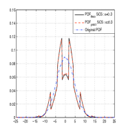
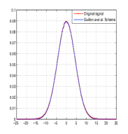
(a)	(b)

Figure 1: (a) Probability density functions of the host and marked signal using SCS for document to watermark ratio equal to 13 dB with $\alpha=0.3$ and (b) the probability density function of stego-signal with Guillon et al. scheme and the original cover-signal.

For $\alpha=1/2$, there are no holes and no aliasing but we obtain a continuous p.d.f. only if $p_{X}(u/2)=p_{X}(u/2+\Delta/4)$. The last equality is satisfied only if the p.d.f. is uniform.

The observed discontinuities lead to a statistical detectable embedding. In the next part, we propose to study an improved scheme based on SCS.

I-A Improvement of SCS: Guillon et al. scheme

By learning from Anderson and Petitcolas’s work [8], Guillon et al. [3] proposed a practical scheme of steganography with public key using asymmetric cryptography and SCS. Fig. 2 summarizes the two phases of this scheme. In the initialization phase, a private key k is generated with a pseudo-random generator and is encrypted with an asymmetric cypher algorithm. The key $C(\textbf{k},\textbf{k}_{\scriptsize\textrm{pub}})$ – where $\textbf{k}_{\scriptsize\textrm{pub}}$ is a public key known by all users – is embedded on the cover-signal. The permanent phase uses the transmitted key k and SCS to embed and transmit the message m.

In the permanent phase, the statistical undetectability is mainly assured by the private key, since it leads to a non distorted p.d.f. However, the initialization phase requires the transmission of public information without distorting the stego-signal. Guillon et al. proposed to use SCS with $\alpha=1/2$ in order to hide an invisible (statistically and perceptually) message, but it is only valid for a cover-signal with uniform p.d.f.; they then proposed to use a compressor before embedding in order to equalize the p.d.f. of cover-content. The embedded message will be statistically invisible, as shown in Fig. 1(b). Unfortunately, the resulting stego-system is less flexible, because the encoding and decoding steps highly depend on the statistics of cover-content. It has been recently shown [4] that the artifacts in the stego-signal are due to the use a regular partitioning codebook. In the next section, we propose to use a structured codebook by the way of TCQ.

Figure 2: Asymmetric steganography scheme: the permanent phase is initialized with a temporary private key k.

II Analysis of the trellis-coded quantization

The approach proposed here concerns the use of a trellis-based quantization, for a pseudo-random partitioning of the codebooks, in order to avoid the artifacts introduced in the p.d.f. of stego-content by regular partitioning (as observed in the previous stego-system).

II-A Principles

Let us consider a trellis defined by a transition function: $\mathcal{E}\times\{0,1\}\longrightarrow\mathcal{E}$, $\textrm{tr}:\left(\textbf{e}[i],\textbf{m}[i]\right)\longmapsto\textbf{e}[i+1]$, with $\mathcal{E}=\{0,1,\ldots,2^{r-1}\}$ groups of possible states, where $r$ is an integer such as $r>1$, and $i$ is the index of current transition. Contrary to the SCS, the dithering d will not be random but will become a function of the current state and of the embedded symbol:

$$\mathcal{E}\times\{0,1\} \longrightarrow [-\Delta/2,+\Delta/2]\textrm{,}$$

$$f:\left(\textbf{e}[i],\textbf{m}[i]\right) \longmapsto \textbf{d}[i]\textrm{.}$$ (2)

In this stego-system, the codebooks are defined by

$$\mathcal{U}_{\textbf{m}}[i]=\left\{n\Delta+f(\textbf{e}[i],\textbf{m}[i])\textrm{,~{}}n\in\mathcal{Z}\right\}\textrm{,}$$

and the closest codeword $\textbf{u}^{\star}\in\mathcal{U}_{\textbf{m}}$ to $\textbf{s}[i]$ is calculated using a Viterbi algorithm [9], with a high a priori in order to be sure that the obtained codeword belongs to $\mathcal{U}_{\textbf{m}}$:

$$\textbf{u}^{\star}=\arg\min_{\textbf{u}\in\mathcal{U}_{\textbf{m}}}\sum_{j=1}^{G}\left(\textbf{s}[j]-\textbf{u}[j]\right)^{2}\textrm{.}$$ (3)

The stego-signal is given by:

$$\textbf{x}=\textbf{s}+\alpha\left(\textbf{u}^{\star}-\textbf{s}\right)\textrm{,}$$ (4)

where s is the cover-signal and $\alpha$ represents the Costa’s parameter.
To extract the embedded message, we have to apply the Viterbi algorithm in order to retrieve the path which corresponds to the stego-signal.

II-B Statistical analysis of TCQ

In order to theoretically justify the use of the TCQ to get statistical invisibility, we have calculated the p.d.f. (see appendix V-B). We obtain:

$$p_{X}(x)=\frac{1}{\sigma_{W}\sqrt{12}}\int_{x-\sigma_{W}\sqrt{3}}^{x+\sigma_{W}\sqrt{3}}p_{S}(z)\textrm{~{}d}z\textrm{,}$$ (5)

where $\sigma_{W}$ is the standard deviation of the embedded signal. Then $p_{X}$ is the mean p.d.f. for the cover signal in the interval centered on $x$ and a width $\sigma_{W}\sqrt{3}$. We have implemented Eqn. (5) for a signal with Gaussian p.d.f. and we obtained the results presented on Fig. 3(a) and 3(b). We can notice the good match between the p.d.f. obtained with the TCQ algorithm (experimental), the theoretical versions and the original ones for the same high embedding power.

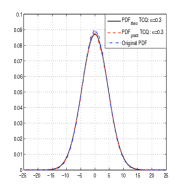
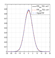
(a)	(b)

Figure 3: Probability density functions of the cover and stego-signal for document to watermark raio equal to 13 dB by using TCQ with different value of $\alpha$: (a) $\alpha=0.3$ and (b) $\alpha=0.7$.

However, Fig. 4(a) shows that the capacity of TCQ is not as good as that of SCS. Then, we can use the TCQ only in the initialization phase – of the previous scheme (Fig. 2) –, because this phase requires just a limited payload.

III Analysis of the spread transform scalar Costa scheme

We propose to use the ST system which allows any stego-system to increase its Watermark-to-Noise Ratio (WNR) [5] and improve the resistance against active warden (who performs an AWGN attack in order to remove the stego-message).

III-A Spread transform

Chen and Wornel [10] introduced a general approach for robust watermarking applications. It allows to spread the embedded message on several cover samples. They proposed to hide the message in a transformed domain [5]. In sequel, the spreading parameter is modeled by a realizations set of random variables with uniform p.d.f. To extract the hidden message, an inverse transformation is applied to a resulted signal.

In [5], authors studied especially the robustness of this system to applied it to the robust watermarking. In this work, we study the steganographic performance of the spread transform system in active warden context. We note that, before transmitted the information, the spread transform makes an inverse transformation where the embedded signal strength is divided by the spreading factor $\tau$, then $\textrm{DWR}=\textrm{DWR}_{\tau}+10\log_{10}\tau$, such as DWR is the Document-to-Watermark Ratio and $\textrm{DWR}_{\tau}$ is the Document-to-transformed Watermark Ratio. Thus, spread transform improves the perceptual invisibility of any hiding system.

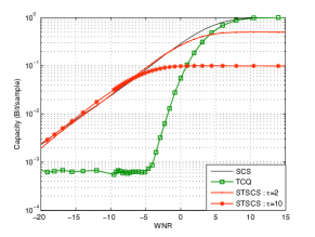
(a)

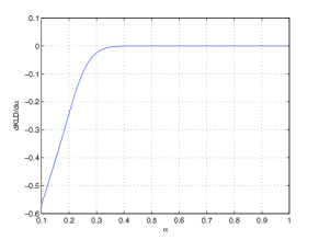
(b)

Figure 4: (a) The capacity of stego-systems SCS, TCQ and ST-SCS as function of watermark to noise ratio and (b) the differentiation of the function $\textrm{kld}(\alpha)$ with respect to the parameter $\alpha$, in the case of ST-SCS stego-system with $\tau=2$.

III-B Statistical analysis of ST-SCS

In sequel, we focus only on the combination of the spread transform with the SCS-based stego-system in active warden context. In order to evaluate the statistical undetectability of the stego-system, we develop a theoretical formulation of ST-SCS stego-signal density (see appendix V-C):

$$p_{X}(x)=\frac{\tau}{4(\tau-\alpha)}$$

$$\sum_{u,m,t}\int_{y}\delta\left(u-Q_{\Delta}\left(\frac{\tau}{\tau-\alpha}\left(x+\alpha yt-\alpha ut\right)t+y\right)\right)$$

$$\times p_{s}\left(\frac{\tau}{\tau-\alpha}\left(x+\alpha yt-\alpha ut\right)\right)p_{Y}(y)\textrm{~{}d}y\textrm{.}$$

In Fig. 5, the experimental p.d.f. of the stego-signal validates the theoretic model given by Eqn. III-B, because we can see that the theoretic p.d.f. follows the experimental one.

If we replace $t$ with its two possible realizations, i.e. $\pm 1/\sqrt{\tau}$, and we take $\tau\rightarrow\infty$ with finite $\sigma_{s}^{2}$ (the variance of cover-signal $s$) then:

$$p_{X}(x) = \frac{1}{4}\sum_{u,m}\int_{y}\delta\left(u-Q_{\Delta}\left(y\right)\right)p_{S}(x)p_{Y}(y)\textrm{~{}d}y$$

$$+\frac{1}{4}\sum_{u,m}\int_{y}\delta\left(u-Q_{\Delta}(y)\right)p_{S}(x)p_{Y}(y)\textrm{~{}d}y\textrm{.}$$

So the stego-signal x has the same density as the cover-signal – in this case the two p.d.f. are both Gaussian. However, Fig. 4(b) shows that the differentiation of the KLD by respect to $\alpha$ is always negative and converges speedily to zero even for $\tau=2$, then the KLD takes – theoretically – its minimal value for the majority values of the parameter $\alpha$ and for any value of the spreading factor $\tau$. In addition, experiences show that the stego-signal has the same p.d.f. than the cover-signal even for a small value of spreading factor $\tau$ (see Fig. 5). We can see on Fig. 6(a), Fig. 7(a) and Fig. 7(b) that ST-SCS has the same level of the statistical undetectability as TCQ stego-system, but better than the undectability level of the SCS.

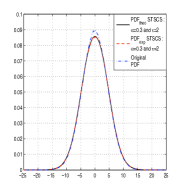
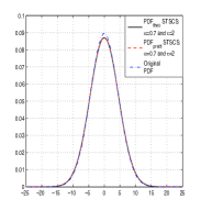
(a)	(b)
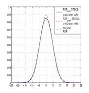
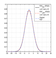
(c)	(d)

Figure 5: Probability density functions of the cover and stego-signal by using ST-SCS for $\tau=2$ and document to watermark ratio equal to 13 dB with different value of $\alpha$: (a) $\alpha=0.3$ and (b) $\alpha=0.7$; for $\tau=10$ with (c) $\alpha=0.3$ and (d) $\alpha=0.7$.

III-C Performance of ST-SCS

Fig. 4(a) shows that for strength warden attack (low WNR), the capacity of ST-SCS is better than the one of TCQ. In the contrary, for high WNR values, the capacity of the TCQ is better. As a result, it is very difficult to have a system which permits a good invisibility and in the same time a good capacity; then the compromise between these two characteristics becomes important. Fig. 6(b) shows that the compromise of ST-SCS is the best in comparison to the SCS and the TCQ stego-systems in active warden context.

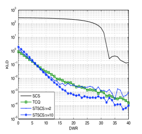
(a)

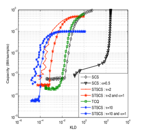
(b)

Figure 6: (a) The Kullback-Leibler distance for SCS, TCQ and ST-SCS stego-systems with Gaussian images as function of DWR; (b) capacity vs. Kullback-Leibler distance for SCS, TCQ and ST-SCS stego-systems with Gaussian images such that WNR $\in[-20,12]$ dB and document-to-watermark ratio $\in[0,40]$ dB.

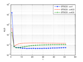
(a)

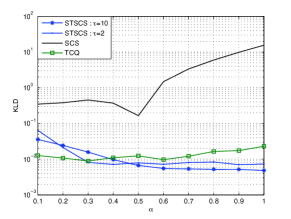
(b)

Figure 7: (a) The Kullback-Leibler distance of ST-SCS as function of $\tau$ for different value of $\alpha$ and (b) the Kullback-Leibler distance as function of $\alpha$ for different value of $\tau$.

We have applied SCS, TCQ-based scheme and ST-SCS to $100$ real images with $350\times 350$ pixels size. Fig. 8 confirms the results obtained for Gaussian images, where the ST-SCS has the same undetectability level as TCQ and better than SCS. However, the statistical undetectability will be the same as SCS in transformed domain if the projection parameter is public.

In the case of public key steganography (Fig. 2), we can use the TCQ stego-system in the initialization phase, to transmit the secret key, and the ST-SCS in the permanent phase, which allows to the best compromise between statistical undetectability and capacity.

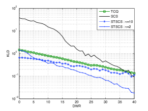
Figure 8: KLD vs. document to watermark ratio with 100 real images of size $350\times 350$.

Conclusion and Perspectives

In this work, we have compared the steganographic performance of several informed-based stego-systems in active warden context. For each system, the experimental results have been used to validate the theoretical model. For SCS, the stego-signal is regularly partitioned, thus, many artifacts in the p.d.f. of the stego-signal are introduced, which is also proved by the developed theoretical formulations. Due to this observations, we have proposed an analysis of two another systems. The first one is based on a pseudo-random partitioning (the TCQ-based system), which allows to obtain a more common and undetectable public stego-system (the technique does not depend to the cover-signal distribution). The second one is based on the combination of SCS with spread transform (the ST-SCS), which allows a good statistical undetectability and a best compromise between capacity and undetectability. In future work, we shall study an improvement of the undetectability with combination of ST and TCQ when the projection parameter is public. We shall also verify our theoretical models by an applications on real images.

IV Acknowledgment

The authors would like to thank Professor Pierre Duhamel for his help and collaboration to this paper and the ESTIVALE project from ANR (French national agency of research) for funding.

V Appendix

V-A Demonstration of Eqn. (1)

We model the stego-signal by a realizations set of Gaussian random variables, independent and non stationary: $\mathcal{X}=\{X[1],\ldots,X[G]\}$. It is given by the following equation (in sequel, we do not use the index of the variable for ease of presentation):

$$X=(1-\alpha)S+\alpha U,$$ (6)

where $\alpha$ represents the Costa’s optimization parameter and a cover-signal is modeled by a realizations set of Gaussian random variables, independents and non stationary: $\mathcal{S}=\{S[1],\ldots,S[G]\}$. According to the product rule

$$p(s|u,m)=\frac{p(u|s,m)p_{S}(s)}{p(u|m)}\textrm{,}$$

we have:

$$p(u|s,m)=\delta(u-Q_{\Delta}(s))\textrm{,}$$ (7)

where $Q_{\Delta}(.)$ represents a scalar quantizer with step $\Delta$. In the other hand,

$$p(s|m)=\sum_{u}p(s|u,m)p(u|m)=\sum_{u}\delta(u-Q_{\Delta}(s))p_{S}(s)\textrm{.}$$

If we replace $S=\frac{X-\alpha U}{1-\alpha}$ in the last equation, we obtain

$$p(x|m)=\frac{1}{1-\alpha}\sum_{u}\delta\left(u-Q_{\Delta}\left(\frac{x-\alpha u}{1-\alpha}\right)\right)p_{S}\left(\frac{x-\alpha u}{1-\alpha}\right)\textrm{.}$$

When the information bits are equiprobable, we write:

$$p_{X}(x)=\frac{1}{2(1-\alpha)}\sum_{u,m}\delta\left(u-Q_{\Delta}\left(\frac{x-\alpha u}{1-\alpha}\right)\right)p_{S}\left(\frac{x-\alpha u}{1-\alpha}\right)\textrm{.}$$

V-B Demonstration of Eqn. (5)

We note $\textbf{e}[i]$ –for $i=1,\ldots,N$ – the trellis states and we suppose that all these states follow an uniform distribution such as : $p_{E}(e)=1/N$. In TCQ-based stego-system, we substitute the cover-samples by $U_{(n,m,e)}$, $n\in\mathcal{Z}$, the codeword of sub-codebook which corresponds to the state $e$ and message-bit $m$. It is given by $U_{(n,m,\textbf{e}[i])}=(n+m/2-i/N)\Delta$ for $i=1,\ldots,N/2$ and $U_{(n,m,\textbf{e}[i])}=U_{n,m,\textbf{e}[i-N/2]}$ for $i=N/2+1,\ldots,N$. By leading on appendix V-A, the p.d.f. formulation of TCQ stego-signal for a fixed state $e$ is :

$$p(x|e)=\frac{1}{2\left(1-\alpha\right)}\sum_{n,m}1_{\left[-\frac{1}{2(1-\alpha)},\frac{1}{2(1-\alpha)}\right]}(x-u_{(n,m,e)})$$

$$\times p_{S}\left(\frac{x-\alpha u_{(n,m,e)}}{1-\alpha}\right)\textrm{,}$$ (8)

and

$$p_{X}(x)=\sum_{i=1}^{N}p_{X}(x|\textbf{e}[i])p_{E}(\textbf{e}[i])$$

$$=\frac{1}{(1-\alpha)}\sum_{n,m}\frac{1}{N}\sum_{i=1}^{N/2}1_{\left[-\frac{1}{2(1-\alpha)},\frac{1}{2(1-\alpha)}\right]}\left(x-u_{(n,m,\textbf{e}[i])}\right)$$

$$\times p_{S}\left(\frac{x-\alpha u_{(n,m,\textbf{e}[i])}}{1-\alpha}\right)\textrm{,}$$ (9)

if the number of states is large and by leading on the properties of the Riemann sum, then:

$$p_{X}(x) = \frac{1}{1-\alpha}$$ (10)

$$\sum_{n,m}\int_{0}^{\frac{1}{2}}1_{\left[-\frac{1}{2(1-\alpha)},\frac{1}{2(1-\alpha)}\right]}\left(x-(n+\frac{m}{2}-\gamma\right)\Delta)$$

$$\times p_{S}\left(\frac{x-\alpha\left(n+\frac{m}{2}-\gamma\right)\Delta}{1-\alpha}\right)\textrm{~{}d}\gamma\textrm{.}$$

If we replace $m$ by its two possible values, i.e. 0 or 1, and make the following variable change $Z=\frac{X-\alpha\gamma\Delta}{1-\alpha}$, we obtain:

$$p_{X}(x)=\frac{1}{\alpha\Delta}\int_{x-\frac{\alpha\Delta}{2}}^{x+\frac{\alpha\Delta}{2}}p_{S}(z)\textrm{~{}d}z=\frac{1}{\sigma_{w}\sqrt{12}}\int_{x-\sigma_{w}\sqrt{3}}^{x+\sigma_{w}\sqrt{3}}p_{S}(z)\textrm{~{}d}z\textrm{.}$$

V-C Demonstration of Eqn. (III-B)

The transformation of the cover-signal is modeled by a realizations set of Gaussian random variables, independents and non stationary, i.e. $\mathcal{S}^{\scriptsize\textrm{st}}=\{S^{\scriptsize\textrm{st}}[1],\ldots,S^{\scriptsize\textrm{st}}[G/\tau]\}$. In addition, we take the spreading direction t such as $\forall i$, $\textbf{t}[i]=\pm\frac{1}{\sqrt{\tau}}$ and it is modeled by a set of Gaussian, independents and non stationary random variables, i.e. $\mathcal{T}=\{T[1],\ldots,T[N]\}$. Then, when the ST-SCS is used to embed the message, the stego-signal $X$ is given by $X=S+\alpha(U-S^{\scriptsize\textrm{st}})T$, if we consider:

$$S_{l}^{\scriptsize\textrm{st}}=\sum_{i=\tau l}^{\tau l+\tau-1}S[i]\times T[i]=S[n]\times T[n]+\underbrace{\sum_{i\neq n}S[i]\times T[i]}_{Y_{n}[l]}\textrm{,}$$

where $Y$ is considered as a random variable modeled by a set $\mathcal{Y}=\{Y_{1}[1],\ldots,Y_{G}[G/\tau]\},$ then

$$X=S+\alpha(U-ST-Y)T\textrm{.}$$ (11)

Since $\textbf{t}[i]=\pm 1/\sqrt{\tau}$ and $\forall i$, $\textbf{t}[i]^{2}=1/\tau$, thus the previous equations becomes

$$X=\left(1-\frac{\alpha}{\tau}\right)S-\alpha YT+\alpha UT\textrm{.}$$ (12)

Now, we compute the p.d.f of the codeword $U$ conditionally to $S$, $Y$, $T$ and the message $m$:

$$p(u|s,y,t,m)=\delta\left(u-Q_{\Delta}\left(st+y\right)\right)\textrm{,}$$ (13)

where $\delta$ represents the Kronecker symbol. Therefore

$$p(s|u,y,t,m)=\frac{\delta\left(u-Q_{\Delta}\left(st+y\right)\right)p(s|y,t,m)}{p(u|y,t,m)}\textrm{.}$$ (14)

In this work, we consider $S$ as a random variable independent of $T$ and $Y$. Therefore $p(s|y,t,m)=p(s)$ and

$$p(s|u,y,t,m)=\frac{\delta\left(u-Q_{\Delta}\left(st+y\right)\right)p_{S}(s)}{p(u|y,t,m)}\textrm{.}$$ (15)

Now, we make the following variable change:

$$S=\frac{\tau}{\tau-\alpha}(X+\alpha T-\alpha UT)\textrm{.}$$ (16)

Then, we obtain

$$p(x|u,y,t,m)=\frac{\tau}{\tau-\alpha}$$

$$\times\frac{\delta\left(u-Q_{\Delta}\left(\frac{\tau}{\tau-\alpha}\left(x+\alpha yt-\alpha ut\right)\right)t+y\right)}{p(u|y,t,m)}$$

$$\times p_{S}\left(\frac{\tau}{\tau-\alpha}\left(x+y-\alpha ut\right)\right)\textrm{,}$$ (17)

Since $T$ is a random variable which the realizations take just two values $\pm 1/\sqrt{\tau}$, and since $m$ is also considered as equiprobable, the marginalization over this two variables and over $U$ and $y$ gives:

$$p_{X}(x)=\frac{\tau}{4\left(\tau-\alpha\right)}$$

$$\sum_{u,m,t}\int_{y}\delta\left(u-Q_{\Delta}\left(\frac{\tau}{\tau-\alpha}\left(x+\alpha yt-\alpha ut\right)t+y\right)\right)$$

$$\times p_{S}\left(\frac{\tau}{\tau-\alpha}\left(x+\alpha yt-\alpha ut\right)\right)p_{Y}(y)\textrm{~{}d}y\textrm{.}$$ (18)

References

- [1] Cox, I. J., Miller, M. L., Bloom, J. A., Fridrich, J. and Kalker, T.: Digital Watermarking and Steganography, Second Edition, Morgan Kaufmann, 2008.
- [2] Simmons, G. J.: The prisonners’ problem and the subliminal channel, in Advances in Cryptology: Proc. of CRYPTO, pp. 51–67, 1984.
- [3] Guillon, P., Furon T. and Duhamel, P.: Applied public-key steganography, in Proc. SPIE Electronic Imaging, San Jose, CA, 2002.
- [4] Le Guelvouit, G.: Trellis-coded quantization for public-key steganography, accepted to IEEE Conf. on Acoustics, Speech and Signal Proc., Mars 2005.
- [5] Eggers, J. J., Baüml, R., Tzchoppe, R. and Girod, B.: Scalar Costa scheme for information embedding, IEEE Trans. on Signal Processing, Apr. 2003.
- [6] Costa, M. H. M.: Writing on dirty paper, IEEE. Trans. on Information Theory, 29(3): 439–441, May 1983.
- [7] Cachin, C.: An information-theoretic model for steganography, in Information Hiding, 1998.
- [8] Anderson, R. J. and Petitcolas, F. A. P.: On the limits of steganography, IEEE Journal of Selected Areas in Communication, vol. 16, no. 4, pp. 474–481, 1998.
- [9] Forney Jr., G. D.: The Viterbi algorithm, in Proceeding IEEE, vol. 61, pp. 268–278, Mar. 1973.
- [10] Chen, B. and Wornell, G. W.: Quantization index modulation: a class of provably good methods for digital watermarking and information embedding, IEEE Trans. Information Theory, vol. 47, pp. 1423–1443, May 2001.