Entanglement entropy and the determination of an unknown quantum state

Abstract

An initial unknown quantum state can be determined with a single measurement apparatus by letting it interact with an auxiliary, “Ancilla”, system as proposed by Allahverdyan, Balian and Nieuwenhuizen [Phys. Rev. Lett. 92, 120402 (2004)]. In the case of two qubits, this procedure allows to reconstruct the initial state of the qubit of interest $S$ by measuring three commuting observables and therefore by means of a single apparatus, for the total system $S+A$ at a later time. The determinant of the matrix of the linear transformation connecting the measurements of three commuting observables at time $t>0$ to the components of the polarization vector of $S$ at time $t=0$ is used as an indicator of the reconstructability of the initial state of the system $S$. We show that a connection between the entanglement entropy of the total system $S+A$ and such a determinant exists, and that for a pure state a vanishing entanglement individuates, without a need for any measurement, those intervals of time for which the reconstruction procedure is least efficient. This property remains valid for a generic dimension of $S$. In the case of a mixed state this connection is lost.

Introduction. The determination of the unknown state of a quantum system is one of the most important issues in the field of quantum information chuang ; hillery ; bennett . For a qubit the estimation of the density matrix involves the measurement of three non-commuting observables, i.e. three successive Stern-Gerlach measurements performed along three orthogonal directions are necessary to determine the components of the Bloch polarization vector $\vec{\rho}$ which determines the state of $S$. In each measurement in fact, the other two components are destroyed. Recently teo , based on a modification of an idea originally introduced in ariano , a procedure was proposed to bypass this limitation by coupling the system to an ancilla system $A$ whose initial state is known. Starting from a factorized condition, a measurement of three commuting observables at time $t$ in the space of the compound system $S+A$ allows to reconstruct the state of the system of interest $S$ at time zero. This is feasible if for the respective Hilbert spaces: $dim\mathcal{H}_{A}\geq dim\mathcal{H}_{S}$ and if the interaction intertwines the two systems so as to give non-zero determinant for the matrix connecting the measured values of the three observables at time $t$ to the components of the vector $\vec{\rho}$ that individuates the state of $S$ at time $t=0$. This procedure requires just on instance of measurement, i.e. one single apparatus (e.g. simultaneously measuring the $z$-components of the Spins of $S$ and $A$ and their product, in the case of $S$ and $A$ being two qubits) and is therefore more economical and was recently implemented experimentally in du .
The procedure extends to a generic dimension of $S$, as explained in teo , by considering two commuting observables, one pertaining to $S$ and the other to $A$ and evaluating, in repeated experiments, the probabilities $P_{ij}$ to have as outcomes the $i^{th}$ eigenvalue of the first observable and the $j^{th}$ for the second one. A linear mapping between such probabilities and the initial density matrix of $S$, ensues. This is expected to be invertible provided that the number of distinct eigenvalues of both the observables is (at least) equal to the dimension of $\mathcal{H}_{S}$, this implies the above mentioned costraint on the dimension of $\mathcal{H}_{A}$. The particular case of a spin-1/2 particle coupled to a laser cavity field, described by the Jaynes-Cummings hamiltonian, important for possible experimental implementations, was considered in mine1 ; bahar2 .

In this article we answer the question of how, fixed a coupling between $S$ and $A$, the entanglement measure provides information on the feasibility and efficiency of the procedure. We analyze the case of $S$ and $A$ being two qubits, and then generalize the arguments to a generic dimension of $S$ and $A$.

Two by two density matrix. Let us consider a spin-$\frac{1}{2}$ $S$ interacting through a generic time independent Hamiltonian $\hat{H}$ with a second spin-$\frac{1}{2}$ : the ancilla system $A$. The total system $S+A$ is set in the following initial state:

$$\hat{\rho}_{T}(0)=\hat{\rho}_{S}(0)\otimes\hat{\rho}_{A}(0)=\frac{\hat{1}+\vec{\rho}\cdot\vec{\hat{\sigma}}}{2}\otimes\frac{\hat{1}+\lambda\hat{s}_{3}}{2}$$ (1)

where the components $\hat{\sigma}_{i}$, with $i=1,2,3$, are the Pauli one half spin operators acting on the Hilbert space $\mathcal{H}_{S}$ of the spin of interest, and $\hat{s}_{j}$ are the analogous operators acting on the Hilbert spin space $\mathcal{H}_{A}$ of the Ancilla. In the case of an initial pure state, $\hat{\rho}_{T}^{2}(0)=\hat{\rho}_{T}(0)$,which means $|\vec{\rho}|^{2}=1$ and $\lambda=\pm 1$. Since the Hamiltonian $\hat{H}$ is time independent the time evolution operator $\hat{U}(t)=e^{-i\hat{H}t}$ is unitary, this implies that if initially the system is described by a pure quantum state, the quantum state remains pure at any following time.

Furthermore, using the properties of the evolution operator, the expectation value of a general operator $O$ at time $t$, acting on the Hilbert space $\mathcal{H}_{S}\otimes\mathcal{H}_{A}$, can be easily calculated as:

$$\langle\hat{O}\rangle_{t}=Tr_{A}[e^{-i\hat{H}t}\hat{\rho}_{T}(0)e^{i\hat{H}t}\hat{O}],$$ (2)

from which it descends that: $\big{(}\mathfrak{i}\big{)}$ $\langle O(t)\rangle$ is just a linear function of $\rho_{1},\rho_{2}$ and $\rho_{3}$, the parameters describing the initial quantum state of the spin of interest and therefore $\big{(}\mathfrak{ii}\big{)}$ no quadratic term, $a_{ij}\rho_{i}\rho_{j}$, appears in the expectation value of a generic operator $\hat{O}$.

We consider, now, two general observables whose operators are: $\hat{O}_{S}$, related to the spin of interest, $\hat{O}_{A}$, related to the Ancilla spin, and the observable related to the operator $\hat{O}_{S}\otimes\hat{O}_{A}$. We are interested in the determinant of the $3\times 3$ matrix $M$, defined by the relation:

$$\vec{p}(t)=\Omega(t)\cdot\vec{\rho}+\vec{k}(t),$$ (3)

where $\vec{y}$ represents the column matrix of elements: $\langle\hat{O}_{S}(t)\rangle$, $\langle\hat{O}_{A}(t)\rangle$ and $\langle\hat{O}_{S}(t)\otimes\hat{O}_{A}(t)\rangle$, $\vec{\rho}$ is the polarization vector in Eq. (1) and $\vec{k}$ is a time dependent column matrix. If the state is initially factorized, according to Eq. (1) the determinant of the matrix $M$ at time $t=0$ is obviously zero. If at a generic later time $t$ the determinant does not vanish, Eq. (3) can be inverted and therefore the initial state of the spin of interest can be derived from the expectation values measured at time $t$.

Since only in the case of pure total state a unique definition of entanglement measure exists, we consider separately the cases of initial pure total state and initial mixed total state, even though in the more general protocol the initial state of the system of interest is totally unknown, including therefore its pure or mixed nature.

We wish to show that in the case of initial pure state a correspondence exists between the vanishing quantum Entanglement and the vanishing determinant of $M$. We will see that a vanishing entanglement gives information about the intervals of time where the reconstruction of the initial state is least efficiently implemented.

The case of initial pure state. Let us consider the total system in a pure state at time $t=0$, i.e. the initial total density matrix is given by the expression of Eq. (1) with $|\vec{\rho}|^{2}=1$ and $\lambda=\pm 1$. Obviously, the system will evolve in time through pure states: $\hat{\rho}_{T}^{2}(t)=\hat{\rho}_{T}(t)$. Let us assume that the quantum entanglement of the pure state $\hat{\rho}_{T}(t)$, vanishes at a certain instant $t^{\ast}$, this way the system is described by the quantum state ket $|\alpha\rangle_{t^{*}}|\beta\rangle_{t^{*}}$, thus, the expectation value of the operator $\hat{O}_{S}\otimes\hat{O}_{A}$ is the product of the expectation values of operators $\hat{O}_{S}$ and $\hat{O}_{A}$:

$$\langle\hat{O}_{S}\otimes\hat{O}_{A}\rangle_{t^{*}}=\langle\hat{O}_{S}\rangle_{t^{*}}\langle\hat{O}_{S}\rangle_{t^{*}}.$$ (4)

which obviously means that the mapping (3) is not invertible since the state of system $S$ is described by three independet parameters while the independent components of vector $\vec{p}$ are only two. More in detail, following Eq. (2), we know that the expectation values of the operators $\hat{O}_{S}$ and $\hat{O}_{A}$ are described by the following linear relations:

$$\langle\hat{O}_{S(A)}\rangle_{t^{*}}=\vec{\gamma}_{S(A)}\cdot\vec{\rho}+\delta_{S(A)},$$ (5)

where $\gamma^{i}_{S}\equiv M_{1,i},\gamma^{i}_{A}\equiv M_{2,i}$ and $\delta_{S(A)}\equiv k_{1(2)}$. According to Eq. (4), we obtain the following expression for the expectation value of $\hat{O}_{S}\otimes\hat{O}_{A}$:

$$\langle\hat{O}_{S}\otimes\hat{O}_{A}\rangle_{t^{*}}=\gamma^{i}_{S}\gamma^{j}_{A}\rho_{i}\rho_{j}+\delta_{S}\gamma^{i}_{A}\rho_{i}+\delta_{A}\gamma^{i}_{S}\rho_{i}+\delta_{S}\delta_{A}.$$ (6)

where sum of repeated indexes is implied. According to the observation $\big{(}\mathfrak{i}\big{)}$, we have $\gamma^{i}_{S}\gamma^{j}_{A}=0$ for every $i,j=1,2,3$; thus, either $\gamma^{i}_{S}=0$, or $\gamma^{i}_{A}=0$, or both $\gamma^{i}_{S}=\gamma^{i}_{A}=0$, for every $i=1,2,3$. In any case, at least one of the first two rows of the matrix $\Omega$ vanishes and the third row is proportional to the non vanishing row; for example, in case the second row vanishes, the third row is $\delta_{S}$ times the first row. This way, we have confirmed that the determinant vanishes: $\Delta(t^{*})\equiv det[\Omega(t^{\ast})]=0$.

Now, we study the time derivative of the determinant through the property:

$$\frac{d}{dt}\Delta(t)\equiv\frac{d}{dt}det[\Omega(t)]=\Omega_{i,j}\frac{d}{dt}{[\Omega(t)]_{i,j}},$$ (7)

where $\left[\Omega(t)\right]_{i,j}$ denotes matrix element of row $i$ and column $j$, and $\Omega_{i,j}$ is the corresponding cofactor. Since one of the first two rows of $\Omega$ vanishes, and since the third row is proportional to the non vanishing row, every cofactor of the matrix $\Omega$ vanishes, which means that, when the quantum Entanglement vanishes, the time derivative of the determinant vanishes too, i.e. $[d\Delta(t)/dt]_{t=t^{\ast}}=0$.

For a generic dimension $N$ of $S$ and $M$ of $A$ as explained in teo one considers two commuting observables with nondegenerate spectrum,one pertaining to $S$ and the other to $A$ which read in their spectral decomposition as $\hat{O}_{S}=\sum_{i=1}^{N}s_{i}\hat{s}_{i}$ and $\hat{O}_{A}=\sum_{j=1}^{M}a_{j}\hat{a}_{j}$ One then evaluates, in repeated experiments, the probabilities

$$P_{ij}=\langle\hat{s}_{i}\otimes\hat{a}_{j}\rangle$$ (8)

to have as outcomes the $i^{th}$ eigenvalue of the first observable and the $j^{th}$ for the second one. A linear mapping between the $N\times M$ component vector ${\bf p}$ such that $p_{\alpha}=P_{ij}$, with $\alpha=\{ij\}$ , and the initial density matrix of $S$, ensues As already mentioned, this mapping is expected to be invertible provided that the number of distinct eigenvalues of both the observables is (at least) equal to the dimension of $\mathcal{H}_{S}$, which implies the constraint $M\geq N$. We consider here the case where the Ancilla system has the same dimension of $S$,i.e. $M=N$. In this case the mapping reads:

$${\bf p}(t)=\Omega(t)\cdot{\bm{\rho}}+{\bf{k}}(t)$$ (9)

where ${\bm{\rho}}$ is the $N^{2}-1$ components vector, containing all the independent parameters characterizing the state of system $S$ at time $t=0$ and $\Omega$ is a $(N^{2}-1)\times(N^{2}-1)$ square matrix. Vector ${\bf p}$ in Eq.(9) is therefore restricted to ist first $N^{2}-1$ components, i.e. the last component $p_{N^{2}}=P_{NN}=\langle\hat{s}_{N}\otimes\hat{a}_{N}\rangle$, being fixed by normalization, is omitted.

For convenience we redefine vector ${\bf p}$ components in Eq. (9)to be

$$p_{\alpha}(t)=\left\{\rule{0.0pt}{18.49411pt}\begin{array}[]{cc}\langle\hat{s}_{i}\otimes\hat{1}\rangle_{t}&i=\alpha=1,\dots,N\\ \langle\hat{1}\otimes\hat{a}_{j}\rangle_{t}&j=2,\dots,N,\;\;\alpha=N+j-1\\ \langle\hat{s}_{i}\otimes\hat{a}_{j}\rangle_{t}&i,j\geq 2,\;\;\alpha=2N,\dots,N^{2}-1\\ \end{array}\right.$$ (10)

which amounts to a linear combination rearrangement of the original $N^{2}-1$ components of ${\bf p}$ leaving therefore the determinant of $\Omega$ unchanged. Observation (i) is still valid for this case, so a generic component $p_{\alpha}$ with $\alpha<N$ can be written as:

$$p_{\alpha}=\langle\hat{s}_{\alpha}\otimes\hat{1}_{A}\rangle_{t}=\lambda^{\alpha}_{j}\rho_{j}+\delta^{\alpha}_{S}$$ (11)

The same is true for the components with $N+1\leq\alpha\leq 2N$

$$p_{\alpha}=\langle\hat{1}_{S}\otimes\hat{a}_{\alpha}\rangle_{t}=\lambda^{\alpha}_{j}\rho_{j}+\delta^{\alpha}_{S}$$ (12)

Again if the initial state is pure and if the quantum entanglement vanishes at time $t^{*}$, then, at this time, the system is described by the quantum state ket $|\alpha\rangle|\beta\rangle$ and therefore

$$\langle\hat{s}_{n}\otimes\hat{a}_{m}\rangle_{t^{*}} = \langle\hat{s}_{n}\rangle_{t^{*}}\langle\hat{a}_{m}\rangle_{t^{*}}=$$

$$= \lambda^{n}_{j}\lambda^{m}_{k}\rho_{j}\rho_{k}+\delta^{m}_{A}\lambda^{n}_{j}\rho_{j}+\delta^{n}_{S}\lambda^{m}_{k}\rho_{k}+\delta^{m}_{A}\delta^{n}_{S}.$$

One easily realizes that the argument used for the two qubits case applies again in similar fashion. In fact following observation (i) $\lambda^{n}_{j}\lambda^{m}_{k}=0$ for all $j,k$ , which means that either $\lambda^{n}_{j}=0$ for every $j$ or $\lambda^{m}_{k}=0$ for every $k$ or $\lambda^{n}_{j}=\lambda^{m}_{k}=0$ for all $j,k$. But this implies that either row $n$ or row $m$ of matrix $\Omega$ vanishes and that the row corrsesponding to $\langle\hat{s}_{n}\otimes\hat{a}_{m}\rangle_{t^{*}}$ is proportional to the non vanishing row between row $n$ and row $m$. Therefore the determinant vanishes as well. The time derivative of the determinant is again given by Eq. (7) Since we know that in the matrix $\Omega$ there are rows with all zeros the only non zero contribution to the determinant of the derivative of $\Omega$ can originate out of cofactors with index corresponding to a vanishing row. But these cofactors in turn will contain either a vanishing row or two rows differing just by a multiplicative factor. Therefore also the derivative of the determinant vanishes.

Thus, we have completed the demonstration that a vanishing quantum Entanglement gives both a vanishing determinant and a vanishing time derivative of the determinant, in case of pure initial state. This means the two following relations are true:

$$if\;\;E\left(\hat{\rho}\right)=0\;\Rightarrow\;\Delta(t^{*})=\frac{d}{dt}\Delta(t^{*})=0$$ (14)

$$if\;\Delta(t^{*})\neq 0\;or\;\frac{d}{dt}\Delta(t^{*})\neq 0\;\Rightarrow E\left(\hat{\rho}\right) \neq 0$$ (15)

The case of initial mixed state. Let us go back to the two q-bits case and consider the case where the time evolution is driven by the following Hamiltonian:

$$\hat{H}=\sum_{i=1}^{4}E_{i}|E_{i}\rangle\langle E_{i}|,$$ (16)

whose eigenvalues and eigenkets are (in units with $\hbar=1$):

$$E_{1}=4,\hskip 10.00002ptE_{2}=2,\hskip 10.00002ptE_{3}=1,\hskip 10.00002ptE_{4}=0,$$ (17)

$$|E_{1}\rangle = |+\rangle_{z}|-\rangle_{z}\;,\hskip 5.0pt|E_{2}\rangle=\frac{1}{\sqrt{2}}\left(|+\rangle_{z}|+\rangle_{z}|-\rangle_{z}|+\rangle_{z}\right)$$ (18)

$$|E_{3}\rangle = |-\rangle_{z}|-\rangle_{z}\;,\hskip 5.0pt|E_{4}\rangle=\frac{1}{\sqrt{2}}\left(|-\rangle_{z}|+\rangle_{z}-|+\rangle_{z}|+\rangle_{z}\right),$$

where $|\pm\rangle_{z}$ are the eigenkets of the $z$-component of the Spin operator. Let us consider, now, the case in which the measurement is performed on the $1/2$-Spin operators $\hat{O}_{S}=O^{0}_{S}\hat{1}+\sum_{i=1}^{3}O^{i}_{S}\hat{\sigma}_{i}$ and $\hat{O}_{A}=O^{0}_{A}\hat{1}+\sum_{j=1}^{3}O^{j}_{S}\hat{s}_{j}$. We observe the time evolution driven by the Hamiltonian (16) in two particular cases in which the observables and the initial state of the system are described by the two following set of parameters:

$$|O^{1}_{A}|>|O^{2}_{A}|,\hskip 1.00006ptO^{1}_{S}=O^{2}_{S}=O^{3}_{S}=1$$

$$\lambda_{1}=0,\hskip 1.00006pt\lambda_{2}=\lambda_{3}=1/4,$$ (19)

$$\rho_{1}=1/\sqrt{2},\hskip 1.00006pt\rho_{2}=1/\sqrt{2},\hskip 1.00006pt\rho_{3}=0,$$

corresponding to the spin of interest initially described by a pure state, and

$$|O^{1}_{A}|>|O^{2}_{A}|,\hskip 1.00006ptO^{1}_{S}=O^{2}_{S}=O^{3}_{S}=1,$$

$$\lambda_{1}=0,\hskip 1.00006pt\lambda_{2}=\lambda_{3}=1/4,$$ (20)

$$\rho_{1}=1/3,\hskip 1.00006pt\rho_{2}=1/4,\hskip 1.00006pt\rho_{3}=1/2,$$

corresponding to the spin of interest initially described by a mixed state, with the ancilla in a mixed state in both cases. After some long but straightforward algebra, we find out that in both cases (Entanglement entropy and the determination of an unknown quantum state) and (Entanglement entropy and the determination of an unknown quantum state), at the time instant $t^{\ast}=\pi/2$, the Entanglement of Formation, woters , vanishes, while the Determinant does not, $\Delta(t^{*})=3\left(O^{A}_{2}O^{A}_{2}-O^{A}_{1}O^{A}_{1}\right)/128>0$. Thus, in general, when the total sistem is initially described by a mixed quantum state, properties (14) and (15) are not true.

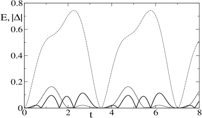
Figure 1: Entanglement $E$ (dashed line) and absolute value of the determinant $|\Delta|$ for two different choices of commuting observables (normal and thick continuous line) vs. time (dimensionless units). Both the system $S$ and the ancilla $A$ are in an initial pure state as given by Eq. (1) with $\rho_{1}=\rho_{2}=0,\rho_{3}=1,\lambda=1$. The interaction is given by Eq. (Entanglement entropy and the determination of an unknown quantum state) with $\cos(2\phi)=1/\sqrt{3}$ as in teo .

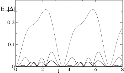
Figure 2: Entanglement of formation $E_{F}$ (dashed line) and absolute value of the determinant $|\Delta|$ for two different choices of commuting observables (normal and thick continuous line) vs. time (dimensionless units). System $S$ is initially in a pure state and the ancilla $A$ in a mixed state, as given by Eq. (1) with $\rho_{1}=\rho_{2}=0,\rho_{3}=1,\lambda=0.5$. The interaction is given by Eq. (Entanglement entropy and the determination of an unknown quantum state) with $\cos(2\phi)=1/\sqrt{3}$ as in teo .

It is obvious that a null entanglement at any time, which implies a factorized condition, implies as well a zero determinant for the matrix $M$ and therefore a condition in which the protocol to measure an initial unknown quantum state here discussed, is not feasible. The reconstructability of the $1/2$ spin of interest depends on the quantum Entanglement with the Ancilla system, generated by the time evolution, so, we would expect a non-vanishing quantum Entanglement to be related to a non-vanishing determinant $\Delta(t)$. Surprisingly, the relation is not so straightforward: only in the case of an initially pure state, a vanishing quantum Entanglement gives both a vanishing determinant and a vanishing time derivative of the determinant. This means that in those instants of time when entanglement vanishes not only the initial state cannot be reconstructed but also that the reconstruction process remains inefficient in immediate future and past times, since the determinant is zero to first order included. So the intervals of time around a time of vanishing entanglement must be avoided in order to have an efficient reconstruction process of the initial state.

In Figs 1 and 2 we plot the entanglement and the determinant for the case of initial pure state and mixed state respectively, adopting for a pure state the standard definition of entanglement $E[\rho_{T}(t)]$

$$E[\rho_{T}(t)]=-Tr[\rho_{S}(t)\log_{2}\rho_{S}(t)]=-Tr[\rho_{A}(t)\log_{2}\rho_{A}(t)]$$

with $\rho_{S}(t)$ and $\rho_{A}(t)$ the partial traces over the system $S$ and the ancilla $A$ respectively. For the mixed state we adopt as entanglement measure the so called ”Entanglement of Formation” $E_{F}$ as originally introduced in woters . The results in both figures refer to the case of $S$ and $A$ interacting through the following operator:

$$\hat{H} = \frac{\hat{\sigma_{1}}}{\sqrt{2}}\otimes(\cos(\phi)\hat{s}_{2}+\sin(\phi)\hat{s}_{3})$$

$$+ \hat{1}\otimes\frac{1}{2}[(\hat{s}_{2}-\hat{s_{1}})\sin(\phi)+\hat{s_{3}}\cos(\phi)]$$

as assumed in teo .

Inverse implication. We wish, now, to study the validity of the inverse implication of (14). To this purpose, we assume that, at a certain instant $t^{\ast}$, the system is described by a quantum state whose Entanglement does not vanish. If we find out that, at least, either the determinant or its time derivative does not vanish, the inverse of implications (14) and (15) is proved. Thus, let us assume that, at a certain instant $t^{\ast}$, the whole quantum system is described by a pure state, $|\Psi\rangle$, whose quantum Entanglement does not vanish. We remind that an orthonormal base set $\left\{|e_{i}\rangle,i=1,2\right\}$ of the Hilbert space $\mathcal{H}_{S}$ and a orthonormal base set $\left\{|f_{i}\rangle,i=1,2\right\}$ of the Hilbert space $\mathcal{H}_{A}$ do exist, such that the following relation holds true:

$$|\Psi\rangle=\sum_{i=1}^{2}\sqrt{\lambda_{i}}|e_{i}\rangle\otimes|f_{i}\rangle$$ (22)

which is the Schmidt SchmidtPF polar form of the quantum state ket $|\Psi\rangle$. Obviously, since the quantum Entanglement of $|\Psi\rangle$ does not vanish, the reduced density matrix has no vanishing eigenvalues, which means: $0<\lambda_{1}=1-\lambda_{2}<1$.

We consider the Schmidt polar form of the state ket $|\Psi\rangle$ and we evaluate the expectation values of the operators $\hat{O}_{S},\hat{O}_{A}$ and $\left(\hat{O}_{S}\otimes\hat{O}_{A}\right)$, given by the following expressions:

$$\langle\hat{O}_{S}\rangle_{t^{*}} = \sum_{j=1}^{2}\lambda_{j}\langle e_{j}|\hat{O}_{S}|e_{j}\rangle$$

$$\quad\langle\hat{O}_{A}\rangle_{t^{*}} = \sum_{j=1}^{2}\lambda_{j}\langle f_{j}|\hat{O}_{A}|f_{j}\rangle,$$ (23)

$$\langle\hat{O}_{S}\otimes\hat{O}_{A}\rangle_{t^{*}} = \sum_{j,k=1}^{2}\sqrt{\lambda_{j}\lambda_{k}}\langle e_{j}|\hat{O}_{S}|e_{k}\rangle\langle f_{j}|\hat{O}_{A}|f_{k}\rangle.$$

Let us consider, now, the particular case where the observables are described by the following hermitian operators: $\hat{O}_{S}=\omega_{1}\left(|e_{1}\rangle\langle e_{2}|+|e_{2}\rangle\langle e_{1}|\right),\quad\hat{O}_{A}=\omega_{2}\left(|f_{1}\rangle\langle f_{2}|+|f_{2}\rangle\langle f_{1}|\right)$. Starting from Eq. (Entanglement entropy and the determination of an unknown quantum state), we easily get the following useful equalities:

$$\langle\hat{O}_{S}\rangle_{t^{*}} = \langle\hat{O}_{A}\rangle_{t^{*}}=0$$ (24)

$$\langle\hat{O}_{S}\otimes\hat{O}_{A}\rangle_{t^{*}} = 2\sqrt{\lambda_{1}\left(1-\lambda_{1}\right)}\omega_{1}\omega_{2},$$

which means that both the first and the second row of the matrix $\Omega$ vanish; thus, according to the relation (7) both the determinant and its time derivative vanish at the instant $t^{\ast}$. So, we have demonstrated that properties described by the inverse of implications (14) and (15), are not true. We stress that the Schmidt polar form depends on the instant $t^{\ast}$, so we need to know the time evolution of the initial state ket in order to find out the particular operators $\hat{O}_{S}$ and $\hat{O}_{A}$ involved in the above demonstration. We also stress a cue point: in case of mixed states, every measure of the quantum Entanglement has to vanish for separable mixed states, i.e. for any ensemble of bipartite factorized quantum states; thus, our results hold true for every measure of the quantum Entanglement.

In conclusion we have considered a protocol for the determination of an unknown quantum state of a system $S$ based on the interaction with an ancilla system $A$, as originally proposed in teo . This protocol allows to determine the initial quantum state of systems $S$ with a single measurement apparatus. Starting from a factorized condition, it is obvious that an interaction entangling the systems $S$ and $A$ is necessary for the protocol to work. Therefore it is natural to think that a connection between Entanglement and the determinant of the linear transformation connecting the parameters individuating the initial quantum state of the system $S$ to the measurement of three (commuting) observables at a later time $t^{*}$ should exist. We find that in the case of initial pure state of both $S$ and $A$ a vanishing entanglement individuates those intervals of time at which the reconstruction process is least efficient. This relation is lost in the case the ancilla system is prepared in an initial mixed state. It is rather surprising that, in the case of a mixed state, even if at a given time $t^{*}>0$ the total density matrix is again separable, interactions exist such that the initial quantum state of the system $S$ can still be recovered from measurements done at this time, and we have provided an example of such interactions. This seems to aim at the long debated different nature between mixed and pure quantum states and at the different physical meaning of entanglement in the two cases.

- (1) I.L. Chuang et al. Nature (London) 393, 143 (1998)
- (2) J. A. Bergou, U Herzog and M. Hillery, Phys. Rev. A. 71, 042314 (2005).
- (3) C. H. Bennett and D. P. Divincenzo, Nature (London) 404, 247 (200)
- (4) Armen E. Allahverdyan, R. Balian and Th. M. Nieuwenhuizen, Phys. Rev. Lett. 92 120402 (2004)
- (5) G. M. D’Ariano, Phys. Lett. A 300,1 (2002).
- (6) Jiangfeng Du, Min Sun, Xinhua Peng and Thomas Durt Phys. Rev. A 74 042341 (2006)
- (7) W. K. Wootters Phys.Rev.Lett. 80 2245 (1998)
- (8) E. Schmidt, Math Ann. 63 (1906) 433
- (9) G. Aquino and B. Mehmani, Proceedings of the Workshop ”Beyond the Quantum”, pp. 115-124, (World Scientific 2007).
- (10) B. Mehmani, A. Allahverdyan and Th. M. Neuwenhuizen, Phys. Rev. A 77, 032122 (2008)