Proximity-driven source of highly spin-polarized ac current on the basis of superconductor/weak ferromagnet/superconductor voltage-biased Josephson junction.

Abstract

We theoretically investigate an opportunity to implement a source of highly spin-polarized ac current on the basis of superconductor/weak ferromagnet/superconductor (SFS) voltage-biased junction in the regime of essential proximity effect and calculate the current flowing through the probe electrode tunnel coupled to the ferromagnetic interlayer region. It is shown that while the polarization of the dc current component is generally small in case of weak exchange field of the ferromagnet, there is an ac component of the current in the system. This ac current is highly spin-polarized and entirely originated from the non-equilibrium proximity effect in the interlayer. The frequency of the current is controlled by the voltage applied to SFS junction. We discuss a possibility to obtain a source of coherent ac currents with a certain phase shift between them by tunnel coupling two probe electrodes at different locations of the interlayer region.

Various proximity and transport phenomena in hybrid structures containing superconducting and ferromagnetic elements are currently in the spotlight. The equilibrium transport and proximity effect in such structures have been theoretically and experimentally investigated recently in details as for the case of weak ferromagnetic alloys (see Ref.buzdin and references therein) so as for half-metals like $CrO_{2}$ Eschrig03 ; Keizer06 .

Spin-dependent properties of nonequilibrium systems are also actively investigated. In particular, the spin imbalance induced in a ferromagnet (F) in nonequilibrium conditions was studied in ferromagnet-superconductor-ferromagnet (FSF) junctions takahashi99 ; maekawa02 ; tserkovnyak02 ; johansson04 ; pena05 ; morten05 . It was found that antiferromagnetic alignment of the exchange fields of the ferromagnets strongly suppresses superconductivity, which leads to large magnetoresistive effect. The influence of the interplay between Andreev reflection at the interface and spin accumulation close to the interface was investigated belzig00 . The effect of spin injection in Josephson junctions was considered takahashi01 . The papers morten05 ; morten04 have theoretically studied the spin relaxation due to spin-flip scattering.

The authors of giazotto05 ; giazotto07 propose the possibility of manipulating magnetization of a mesoscopic normal (N) region through the Zeeman splitting of superconducting density of states and applied voltage in voltage biased SNS or FSNSF tunnel junctions. Also, the spin-polarized transport through superconductor-normal metal hybrid structures, where the density of states in a superconductor is Zeeman-splitted, was investigated giazotto05 ; giazotto07 ; giazotto07a . It was shown that, in alternative to half-metallic ferromagnets, such junction can be used to generate highly spin-polarized currents, which are tunable in magnitude and sign by the bias voltage and exchange field. In giazotto05 ; giazotto07 the normal metal region between the superconducting leads has been considered to be long enough in order to suppress the proximity effect and, consequently, ac Josephson effect in it. However, if the junction length is of the order of superconducting coherence length $\xi=\sqrt{\hbar D/\Delta}$, where $D$ is the diffusion constant and $\Delta$ is the superconducting order parameter in the leads, the interplay between the proximity effect and the Zeeman exchange field in the interlayer can lead to a number of novel qualitative effects. In particular, it was shown that by tunnel coupling of the normal regions of two superconductor-normal metal-ferromagnet trilayers the absolute spin-valve effect can be realized for a certain interval of voltages applied between the normal regions hernando02 . For voltage-biased superconductor-weak ferromagnet-superconductor Josephson junction the interplay between the proximity effect and the Zeeman exchange field results in additional peak-like features in the I-V characteristics bobkovy06 . The ac Josephson current in superconductor-ferromagnet-superconductor voltage biased junction was also studied hikino08 .

In the present paper we study voltage-biased superconductor-weak ferromagnet-superconductor (SFS) Josephson junction focusing on the short enough interlayer (which is considered to be of the order of superconducting coherence length). In this regime the proximity effect between ferromagnet and superconductors is essential. One of the well-known manifestations of the proximity effect, which already takes place in equilibrium, is the so-called minigap in the local density of states (LDOS) of the interlayer mcmillan68 ; Fazio99 . Another important manifestation of the proximity effect is an ac current, which appears in case of voltage-biased junction. We show that the interplay of two above mentioned phenomena in non-equilibrium SFS Josephson junction gives an opportunity to implement a source of highly spin-polarized ac current by tunnel coupling the interlayer region to an additional electrode. The frequency of this ac current is controlled by the voltage $V$, applied to the SFS junction. In addition the proximity effect in the interlayer causes substantial non-linearities in the $I-V_{p}$ characteristics of the ac current flowing through the additional electrode. Here $V_{p}$ is the potential of the probe electrode. The dc current flowing through the additional electrode is also considered, although its spin polarization is obtained to be rather weak except for some narrow ranges of $V_{p}$. We also discuss the phase difference between the ac current flowing through the probe electrode and the ac Josephson current flowing across the SFS junction and show that it depends on the position in the interlayer. Therefore the system under consideration can be used as a source of phase-shifted coherent ac currents by tunnel coupling of two probe electrodes at different locations of the interlayer region.

Further the model and the method we use are described. We study a voltage-biased SFS junction, where F is a diffusive weak ferromagnet of length $d$ coupled to two identical superconducting reservoirs. The superconductors are supposed to be diffusive and have $s$-wave pairing. We assume the SF interfaces to be not fully transparent and suppose that the resistance of the SF boundary $R_{g}$ dominates the resistance of the ferromagnetic interlayer $R_{F}$. We assume the parameter $(R_{F}/R_{g})(\sigma_{F}/\sigma_{s})$, where $\sigma_{F}$ and $\sigma_{s}$ stand for conductivities of ferromagnetic and superconducting materials respectively, to be also small, what allows us to neglect the suppression of the superconducting order parameter in the S leads near the interface. In addition, a normal voltage-biased ”probe” terminal is tunnel coupled to the interlayer through a junction of a resistance $R_{p}\gg R_{g}$.

We use the quasiclassical theory of superconductivity for diffusive systems in terms of time-dependent Usadel equations usadel . The fundamental quantity for diffusive transport is the momentum average of the quasiclassical Green’s function $\check{g}(x,\varepsilon,t)=\langle\check{g}(\bm{p}_{f},x,\varepsilon,t)\rangle_{\bm{p}_{f}}$. It is a $8\times 8$ matrix form in the product space of Keldysh, particle-hole and spin variables. In general the quasiclassical Green’s functions depend on space $\bm{R}$, time $t$ variables and the excitation energy $\varepsilon$. The considered problem is effectively one-dimensional and $\bm{R}\equiv x$, where $x$ - is the coordinate measured along the normal to the junction.

The quasiclassical Green’s function $\check{g}(x,\varepsilon,t)$ satisfies the non-stationary Usadel equation, which in the ferromagnetic region takes the form

$$\left[\varepsilon\hat{\tau}_{3}-\check{\Sigma}(x,\varepsilon,t),\check{g}\right]_{\otimes}+\frac{D}{\pi}\partial_{x}\left(\check{g}\otimes\partial_{x}\check{g}\right)=0\enspace,$$ (1)

supplemented by the normalization condition

$$\check{g}\otimes\check{g}=-\pi^{2}\enspace.$$ (2)

The product $\otimes$ of two functions of energy and time is defined by the noncommutative convolution $A\otimes B=e^{i(\partial_{\varepsilon}^{A}\partial_{t}^{B}-\partial_{t}^{A}\partial_{\varepsilon}^{B})/2}A(\varepsilon,t)B(\varepsilon,t)$. In the problem we consider the self-energy takes the form $\check{\Sigma}(x,\varepsilon,t)=h\hat{\sigma}_{3}$, where $h$ is an exchange field in the ferromagnet. $\hat{\tau}_{i}$ and $\hat{\sigma}_{i}$ are Pauli matrices in particle-hole and spin spaces, respectively.

In order to solve the Usadel equation it is convenient to express quasiclassical Green’s function $\check{g}$ in terms of Riccati coherence functions $\hat{\gamma}^{R,A}$ and $\hat{\tilde{\gamma}}^{R,A}$, which measure the relative amplitudes for normal-state quasiparticle and quasihole excitations and distribution functions $\hat{x}^{K}$ and $\hat{\tilde{x}}^{K}$. All these functions are $2\times 2$ matrices in spin space and depend on $(x,\varepsilon,t)$. The corresponding expression for $\check{g}$ takes the formEschrig00

$$\check{g}^{R,A}=\left(\begin{array}[]{cc}\hat{g}^{R,A}&\hat{f}^{R,A}\\ \hat{\tilde{f}}^{R,A}&\hat{\tilde{g}}^{R,A}\end{array}\right)=\mp i\pi\check{N}^{R,A}\otimes$$

$$\otimes\left(\begin{array}[]{cc}(1+\hat{\gamma}^{R,A}\otimes\hat{\tilde{\gamma}}^{R,A})&2\gamma^{R,A}\\ -2\hat{\tilde{\gamma}}^{R,A}&-(1+\hat{\tilde{\gamma}}^{R,A}\hat{\gamma}^{R,A})\end{array}\right)\enspace,$$ (3)

$$\check{g}^{K}=\left(\begin{array}[]{cc}\hat{g}^{K}&\hat{f}^{K}\\ -\hat{\tilde{f}}^{K}&-\hat{\tilde{g}}^{K}\end{array}\right)=-2i\pi\check{N}^{R}\otimes$$

$$\left(\!\!\!\!\begin{array}[]{cc}(\hat{x}^{K}-\hat{\gamma}^{R}\otimes\hat{\tilde{x}}^{K}\otimes\hat{\tilde{\gamma}}^{A})\!\!\!\!\!&-(\hat{\gamma}^{R}\otimes\hat{\tilde{x}}^{K}-\hat{x}^{K}\otimes\hat{\gamma}^{A}\\ -(\hat{\tilde{\gamma}}^{R}\otimes\hat{x}^{K}-\hat{\tilde{x}}^{K}\otimes\hat{\tilde{\gamma}}^{A})\!\!\!\!\!&(\hat{\tilde{x}}^{K}-\hat{\tilde{\gamma}}^{R}\otimes\hat{x}^{K}\otimes\hat{\gamma}^{A})\end{array}\!\!\!\right)\!\otimes\check{N}^{A},$$ (4)

$$\check{N}^{R,A}\!=\!\left(\!\!\!\!\begin{array}[]{cc}\left(1-\hat{\gamma}^{R,A}\otimes\hat{\tilde{\gamma}}^{R,A}\right)^{-1}\!\!\!\!\!\!&0\\ 0\!\!\!\!\!\!&\left(1-\hat{\tilde{\gamma}}^{R,A}\otimes\hat{\gamma}^{R,A}\right)^{-1}\end{array}\!\!\!\!\right).$$ (5)

Riccati coherence and distribution functions obey Riccati-type transport equationsEschrig00 ; Eschrig04 . For the considered problem in the ferromagnetic region the equations read as follows

$$2\varepsilon\otimes\hat{\gamma}^{R}-[h\hat{\sigma}_{3},\hat{\gamma}^{R}]-$$

$$-iD\left[\partial_{x}^{2}\hat{\gamma}^{R}+\partial_{x}\hat{\gamma}^{R}\otimes\frac{\hat{\tilde{f}}^{R}}{i\pi}\otimes\partial_{x}\hat{\gamma}^{R}\right]=0\enspace,$$ (6)

$$\partial_{t}\hat{x}^{K}-D\left[\partial_{x}\hat{\gamma}^{R}\otimes\frac{\hat{\tilde{f}}^{R}}{i\pi}\otimes\partial_{x}\hat{x}^{K}-\partial_{x}\hat{\gamma}^{R}\otimes\frac{\hat{\tilde{g}}^{K}}{i\pi}\otimes\partial_{x}\hat{\tilde{\gamma}}^{A}+\right.$$

$$\left.+\partial_{x}^{2}\hat{x}^{K}+\partial_{x}\hat{x}^{K}\otimes\frac{\hat{f}^{A}}{i\pi}\otimes\partial_{x}\hat{\tilde{\gamma}}^{A}\right]=0\enspace.$$ (7)

Particle-hole conjugation, denoted by $\tilde{~}{}$, is defined by the operation $\tilde{a}(x,\varepsilon,t)=a(x,-\varepsilon,t)^{*}$. In addition to the conjugation symmetry, the coherence and distribution functions obey the following symmetries $\hat{\gamma}^{A}(x,\varepsilon,t)=\hat{\tilde{\gamma}}^{R}(x,\varepsilon,t)^{\dagger}$, $\hat{x}^{K}(x,\varepsilon,t)=\hat{x}^{K}(x,\varepsilon,t)^{\dagger}$.

Eqs. (6),(7) should be solved together with the boundary conditions at SF interfaces. As it was mentioned above we consider the case when the dimensionless conductance of the boundary $G=R_{F}/R_{g}\lesssim 1$, so the interface transparency $T_{SF}\sim G(l/d)\ll 1$. Due to the smallness of the interface transparency $T$ we can use Kupriyanov-Lukichev boundary conditions at SF boundariesKupriyanov . In terms of Riccati coherence and distribution functions they take the form

$$\partial_{x}\hat{\gamma}^{R}_{l,r}=\pm\frac{G}{2i\pi d}\left[\hat{f}^{R}_{S;l,r}+\hat{\gamma}^{R}_{l,r}\otimes\hat{\tilde{g}}^{R}_{S;l,r}-\right.$$

$$\left.-(\hat{g}^{R}_{S;l,r}+\hat{\gamma}^{R}_{l,r}\otimes\hat{\tilde{f}}^{R}_{S;l,r})\otimes\hat{\gamma}^{R}_{l,r}\right]\enspace,$$ (8)

$$\partial_{x}\hat{x}^{K}_{l,r}=\pm\frac{G}{2i\pi d}\left[\frac{1}{2}\left(\hat{g}^{K}_{S;l,r}+\hat{\gamma}^{R}_{l,r}\otimes\hat{\tilde{g}}^{K}_{S;l,r}\otimes\hat{\tilde{\gamma}}^{A}_{l,r}\right)-\right.$$

$$\left.-\hat{\gamma}^{R}_{l,r}\otimes\hat{\tilde{f}}^{K}_{S;l,r}-\left(\hat{g}^{R}_{S;l,r}+\hat{\gamma}^{R}_{l,r}\otimes\hat{\tilde{f}}^{R}_{S;l,r}\right)\otimes\hat{x}^{K}_{l,r}-h.c.\right]\enspace.$$ (9)

Here Riccati coherence and distribution functions denoted by the lower case symbols $l,r$ are taken at the left and right ends of the ferromagnet. The quantities denoted by the lower case symbols ($S;l,r$) are corresponding Green’s functions at the superconducting side of the left and right SF interfaces. As it was already mentioned above, under the condition $(R_{F}/R_{g})(\sigma_{F}/\sigma_{s})\ll 1$ we can neglect the suppression of superconducting order parameter in the leads and, moreover, take the Green’s functions at the superconducting side of the boundaries to be equal to their bulk values, which can be easily deduced from the expressions (3) and (4) using the following bulk values of Riccati coherence and distribution functions

$$\hat{\gamma}_{S;l,r}^{R,A}=\left\{\begin{array}[]{ll}\frac{\displaystyle\Delta e^{-2ieV_{l,r}t}}{\displaystyle\varepsilon\pm i\sqrt{\Delta^{2}-\varepsilon^{2}}}i\hat{\sigma}_{2},&|\varepsilon|<\Delta\\ \frac{\displaystyle\Delta e^{-2ieV_{l,r}t}}{\displaystyle\epsilon+{\rm sgn\varepsilon}\sqrt{\varepsilon^{2}-\Delta^{2}}}i\hat{\sigma}_{2},&|\varepsilon|>\Delta\enspace,\\ \end{array}\right.$$ (10)

$$\hat{x}_{S;l,r}^{K}=\left(1-|\hat{\gamma}_{l,r}^{R}(\varepsilon-eV_{l,r})|^{2}\right)\tanh\frac{\varepsilon-eV_{l,r}}{2T}\enspace,$$ (11)

$\Delta$ is the superconducting order parameter absolute value in the bulk, which is assumed to be the same in the both superconductors. $V_{l,r}$ is the electric potential in the bulk of left (right) superconductor, so $V=V_{r}-V_{l}$ is the voltage bias applied to the junction. $T$ is the temperature.

The electric and spin currents flowing through the probe electrode should be found via Keldysh part of the quasiclassical Green’s function. It is convenient to calculate the currents in the probe electrode. Given the quasiclassical Green’s function $\check{g}_{p}({\bm{p}}_{f},\varepsilon,t)$ at the interface of the probe electrode the corresponding expression for the electric current reads as follows

$$\frac{j^{el}}{e}\!=\!\left\langle\!N_{f}v_{f,y}\!\!\!\int\limits_{-\infty}^{+\infty}\!\!\!\frac{d\varepsilon}{4\pi i}{\rm Tr}_{4}\left[\frac{(\hat{\tau}_{0}+\hat{\tau}_{3})}{2}\hat{\sigma}_{0}\check{g}^{K}_{p}({\bm{p}}_{f},x,\varepsilon,t)\right]\right\rangle_{{\bm{p}}_{f}}.$$ (12)

where $e$ is the electron charge and $\hbar=1$ throughout the paper. The spin current $j^{sp}/s^{e}$ can be calculated making use of Eq. (12) with the substitution $\hat{\sigma}_{3}$ for $\hat{\sigma}_{0}$. $s^{e}=1/2$ is the electron spin. In Eq. (12) $v_{f,y}$ is the Fermi velocity component normal to the junction between the interlayer and the probe electrode, $N_{f}$ is the density of the states on the Fermi level in the probe electrode, $\langle...\rangle_{{\bm{p}}_{f}}=\int\limits_{FS}d\Omega/4\pi$ denotes average over the Fermi surface.

In the first order on the transparency $T_{FP}$ of the junction between the interlayer and the probe electrode (which is considered to be small) the difference between the Green’s functions for an incoming ${\bm{p}}_{f}$ and outgoing ${\underline{\bm{p}}}_{f}$ quasiparticle trajectories $\check{g}_{p}({\bm{p}}_{f},x,\varepsilon,t)-\check{g}_{p}({\underline{\bm{p}}}_{f},x,\varepsilon,t)$ entering Eq. (12) can be expressed in terms of the Green’s functions corresponding to the uncoupled interlayer and probe electrode regions as follows mrs88

$$\check{g}_{p}({\bm{p}}_{f},x,\varepsilon,t)-\check{g}_{p}({\underline{\bm{p}}}_{f},x,\varepsilon,t)=$$

$$=-\frac{iT_{FP}}{2\pi}\left[\check{g}_{F}({\bm{p}}_{f},x,\varepsilon,t),\check{g}_{p}^{(0)}({\bm{p}}_{f},\varepsilon,t)\right]_{\otimes}\enspace.$$ (13)

Here the Green’s function $\check{g}_{F}({\bm{p}}_{f},x,\varepsilon,t)$ in the dirty ferromagnetic interlayer is only slightly dependent on the momentum direction on the Fermi surface and approximately equal to its momentum average value $\check{g}_{F}(x,\varepsilon,t)$. $[A,B]_{\otimes}$ means the commutator $A\otimes B-B\otimes A$. Substituting Eq. (13) into the expression for the current (12) and taking into accout the explicit form of the Green’s function for the uncoupled normal probe electrode $\check{g}_{p}^{(0)R,A}=\mp i\pi\hat{\tau}_{3}\hat{\sigma}_{0}$ and $g_{p}^{(0)K}=-2i\pi\tanh[(\varepsilon-eV_{p})/2T]\hat{\tau}_{3}\hat{\sigma}_{0}$, we get the current flowing through this electrode:

$$j^{el}=\frac{1}{eR_{p}}\int\limits_{-\infty}^{\infty}\frac{d\varepsilon}{4\pi i}{\rm Tr}_{2}\hat{\sigma}_{0}\Bigl{\{}\hat{g}_{F}^{K}(x,\varepsilon,t)+$$

$$\tanh\frac{\varepsilon-eV_{p}}{2T}\otimes\hat{g}_{F}^{A}(x,\varepsilon,t)-\hat{g}_{F}^{R}(x,\varepsilon,t)\otimes\tanh\frac{\varepsilon-eV_{p}}{2T}\Bigr{\}}\enspace.$$ (14)

$\hat{g}_{F}^{R,A,K}(x,\varepsilon,t)$ is the upper left part of the interlayer Green’s function $\check{g}_{F}^{R,A,K}(x,\varepsilon,t)$ in the particle-hole space. The spin current $j^{sp}/s^{e}$ can be calculated from Eq. (14) with the substitution $\hat{\sigma}_{3}$ for $\hat{\sigma}_{0}$. In Eq. (14) the resistance of the interface between the interlayer and the probe electrode $R_{p}^{-1}=e^{2}\int_{v_{f,y}>0}(d\Omega/4\pi)v_{f,y}N_{f,y}T_{FP}$.

The Green’s functions $\check{g}_{F}^{R,A,K}(x,\varepsilon,t)$ are calculated making use of the Riccati-parameterization technique described above. The time dependence of the superconducting order parameter in the leads $\sim\Delta e^{2ieVt}$, which cannot be removed by the gauge transformation in the case of voltage-biased SFS junction, give rise to time dependence of the Green’s function in the interlayer:

$$\check{g}_{F}^{R,A,K}(x,\varepsilon,t)=\sum\limits_{m=-\infty}^{\infty}\check{g}_{m}^{R,A,K}(x,\varepsilon)e^{2iemVt}\enspace.$$ (15)

If the interlayer is long in comparison with the coherence length, all the Green’s function harmonics corresponding to $m\neq 0$ are negligible. This leads, in particular, to the suppression of the ac Josephson effect in SFS junction. However, if the length of the interlayer is of the order of the coherence length, the non-zero harmonics are important and give rise not only to ac Josephson effect, but also to ac electric and spin currents flowing through the probe electrode. It is worth to note here that we consider exchange fields, which are very weak as compared to the Fermi energy $\varepsilon_{F}$ and calculate all the currents to zero order of the parameter $h/\varepsilon_{F}$. In this approximation the spin current across SFS junction is absent (it only appears in the first order of this parameter). At the same time non-zero spin current flows through the probe electrode. The qualitative reason for this effect is the manifestation of the proximity induced minigap, which is splitted by the exchange field, in the essentially nonequilibrium electron distribution function in the interlayer. This is discussed in detail below.

At first, let us focus on the behavior of the dc component of the electric and spin currents flowing through the probe electrode. The differential conductance $dI/dV$ of the electric current (normalized to its asymptotic value $1/R_{p}$ corresponding to high enough $|V_{p}|$) in dependence on $V_{p}$ is plotted in Figs. 1(a) and 2(a). The offset is for clarity. Figs. 1(b) and 2(b) represent the dependence of the dc spin current on $V_{p}$. Fig. 2 demonstrates how these quantities are affected by the exchange field, while Figs. 1(a)-(b) show the influence of voltage $V$ applied to SFS junction.

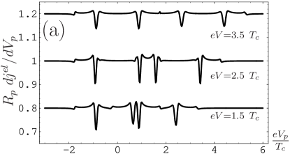
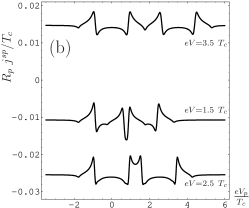
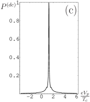
Figure 1: (a) The differential conductance of the dc electric current flowing through the probe electrode as a function of $eV_{p}$. Different curves are related to three different values of the voltage $V$, applied to SFS junction. The conductance is normalized to its asymptotic value $1/R_{p}$ corresponding to high enough $|V_{p}|$. The offset is for clarity. (b) The dependence of the dc spin current on $eV_{p}$ for the same three values of $V$. There is no offset. The spin current is measured in units of $T_{c}/R_{p}$, where $T_{c}$ is the critical temperature of the superconducting leads. (c) The degree of spin polarization $P^{(dc)}$ of the dc current for $eV=2.5T_{c}$. For other values of the voltage $V$ the behavior of $P^{(dc)}$ is qualitatively the same. The other parameters of the junction are the following: $h=0.9T_{c}$, $d=0.94\xi$, $G=0.04$. All the results presented in the paper are calculated for the temperature $T=0.01T_{c}$.

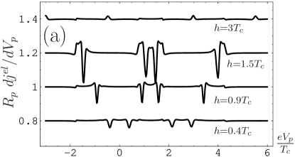
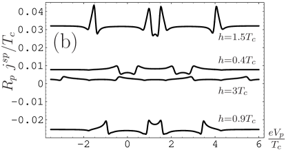
Figure 2: (a) The differential conductance of the dc electric current flowing through the probe electrode as a function of $eV_{p}$. Different curves are related to four different values of exchange field $h$. The offset is for clarity. (b) The dependence of the dc spin current on $eV_{p}$ for the same values of $h$. There is no offset. The other parameters of the junction are the following: $eV=2.5T_{c}$, $d=0.94\xi$ and $G=0.04$.

The most interesting feature of the electric current is series of dips in the differential conductance, which is seen in Figs. 1(a) and 2(a). These dips are direct consequence of the proximity effect and reflect the spin-split minigaps in the LDOS extended from the left interface (corresponding to the voltages $V_{p}=\pm h$) and from the right one (located at the positions $V_{p}=V\pm h$). The sign $\pm$ is related to the different spin subbands. It is seen in Fig. 1(a) that the relative positions of the dip pairs can be adjusted by manipulating the voltage $V$ applied to SFS, which is easily controlled experimentally. Fig. 2(a) demonstrates that these features are the most pronounced for weak exchange fields $h\lesssim\Delta$. For $h>\Delta$ the minigaps are pushed out from the subgap regions of the LDOS and convert into obscure features. Consequently, the dips in the differential conductance become evanescent for high enough exchange fields.

For weak exchange fields $h\lesssim\Delta$ the dc spin current, which is represented in Figs. 1(b) and 2(b), is also a highly non-linear function of $eV_{p}$ if it is roughly between $-\Delta$ and $\Delta+eV$. This is again the consequence of the interplay between the minigaps extended from the both interfaces of the ferromagnet. It is worth to note here that the whole picture is symmetrical with respect to $V_{p}-V/2\to-(V_{p}-V/2)$. The reason is that the curves, represented in Figs. 1 and 2, are obtained at $x=d/2$, that is exactly in the middle of the interlayer. If one would calculate the currents flowing through the probe electrode closer to one of the interfaces, there would be an asymmetry of the corresponding curves with respect to $V_{p}-V/2\to-(V_{p}-V/2)$. This asymmetry originates from the fact that the proximity features extended from the nearest boundary dominate the proximity features, which extended from the other one. It is seen in Fig. 1(b) that the distance between the non-linear features in the spin current is again can be controlled by the voltage $V$. Another non-trivial characteristic feature is that the dc spin current tends to a constant value at large enough $|V_{p}|$ instead of to be a linear function of the voltage bias. This constant value is a non-monotonous function of the exchange field and declines upon increasing $h$ (just as the amplitude of the non-linear features does). This behavior is a consequence of the manifestation of spin-split minigap in the nonequilibrium quasiparticle distribution function in the interlayer and is discussed qualitatively below. However, it is obvious that full dc spin current does not vanish upon increasing $h$ if one takes into account the contributions of the first and the following orders of $h/\varepsilon_{F}$, which are disregarded here but become essential for larger exchange fields.

Fig. 1(c) demonstrates the degree of spin polarization of the current as a function of $V_{p}$. For the dc component of the current this quantity is defined as

$$P^{(dc)}=\frac{|j^{sp}|/s^{e}}{|j_{\uparrow}|+|j_{\downarrow}|}\equiv\frac{|j_{\uparrow}-j_{\downarrow}|}{|j_{\uparrow}|+|j_{\downarrow}|}\enspace,$$ (16)

where $j_{\uparrow(\downarrow)}$ is dc component of the current of spin-up (spin-down) electrons, which can be calculated according to Eq. (14) with the substitution $(\hat{\sigma}_{0}+\hat{\sigma}_{3})/2$ ($(\hat{\sigma}_{0}-\hat{\sigma}_{3})/2$) for $\hat{\sigma}_{0}$. It is seen that the polarization of the dc current is weak everywhere except for the particular narrow ranges of $V_{p}$, where the electric current is small due to smallness of the voltage bias $V_{p}-V/2$ applied between the interlayer and the probe electrode.

Now we turn to the discussion of ac current. Fig. 3 is a representative example of the dependencies of ac electric and spin currents on $V_{p}$. Panel (a) demonstrates the currents in the middle of the interlayer (at $x=d/2$), while the currents at the left interface ($x=0$) are plotted in panel (b). We only consider the first harmonics of ac current, corresponding to $m=\pm 1$ in Eq. (15). The following harmonics are negligible because we assume the transparency of SF interfaces to be low enough, what leads to the suppression of a Green’s function component $g_{m+1}$ by a factor of $G$ with respect to $g_{m}$. Therefore, the electric and spin ac currents can be expressed by $j^{ac,el(sp)}(t)=j^{el(sp)}_{1}e^{2ieVt}+j^{el(sp)}_{-1}e^{-2ieVt}$. Then the amplitudes of these currents, which are represented in Fig. 3, take the form $|j^{ac,el(sp)}|=|j^{el(sp)}_{1}|+|j^{el(sp)}_{-1}|$.

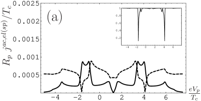
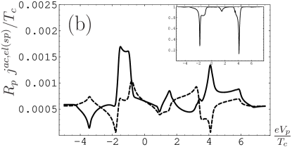
Figure 3: The dependencies of the ac electric (solid line) and ac spin (dashed line) currents on $V_{p}$. $h=0.9T_{c}$, $V=2.5T_{c}$, other parameters of SFS junction are the same as in Figs. 1 and 2. Panel (a) demonstrates the results for the case when the probe electrode is coupled to the interlayer at $x=d/2$, while the curves, represented in panel (b) are calculated at $x=0$.

Similar to the dc currents, $|j^{ac,el(sp)}|$ exhibit quite strong non-linearities if $V_{p}$ is between $-(\Delta+eV)$ and $\Delta+2eV$. The ac spin current also tends to a constant value beyond this interval. This limiting value of the current is also a non-monotonous function of the exchange field and declines upon increasing $h$, as for the case of the dc spin current. However, unlike the dc spin current, it does not contain any contributions, which rise upon increasing $h$. The ac spin current is entirely originated from the non-equilibrium proximity effect and, consequently, is suppressed for the exchange fields, which are considerably larger than $\Delta$. For $h=4.5T_{c}$ the ac spin current is suppressed by a factor $\sim 4$ with respect to the case of $h=0.9T_{c}$, illustrated in Fig. 3.

As concerns the limiting behavior of the ac electric current, it is very different from the dc one: it also saturates at a constant value instead of to be a linear function of $V_{p}$. This limiting value of the ac electric current is comparable to or in most part of cases even less than the limiting value of the spin current. In particular, in the middle of the interlayer (at $x=d/2$) the limiting value of the electric current is negligible (see Fig. 3(a)). Therefore, the ac current is highly spin-polarized practically for the whole parameter range we consider. We define the polarization of the ac current by the following way

$$P^{(ac)}=\frac{\langle|j^{ac,sp}(t)|P(t)\rangle}{\langle|j^{ac,sp}(t)|\rangle}\enspace,$$ (17)

where $\langle...\rangle$ means averaging over time and $P(t)$ is the instantaneous spin polarization of the ac current, defined similar to the polarization of dc current Eq. (16):

$$P(t)=\frac{|j^{ac,sp}(t)|/s^{e}}{|j^{ac}_{\uparrow}(t)|+|j^{ac}_{\downarrow}(t)|}\enspace.$$ (18)

The degree of ac current spin polarization, calculated according to Eq. (17), is represented in inserts to Figs. 3(a) and 3(b) at $x=d/2$ and $x=0$, respectively. It is worth to note here that although the ac spin current declines upon increasing $h$, the exchange field also suppresses the ac electric current. For this reason the spin polarization of the ac current remains to be high even for the case of exchange fields $h>\Delta$. Another factor, which suppresses the proximity effect in the interlayer is considerable increase of the voltage $V$ with respect to $\Delta$.

As it was already mentioned above, all the most essential features of the current flowing through the probe electrode in the system under consideration (behavior of dc spin and ac electric and spin currents, high spin polarization of the ac current) originate from the manifestation of spin-split proximity minigaps in the non-equilibrium distribution function for electrons in the interlayer. In order to get insight into qualitative behavior of this distribution function one can make use of a balance equation. It cannot be applicable for quantitative consideration of the discussed problem even in case if the interlayer is short enough to justify disregarding the inelastic relaxation processes. Nevertheless, it can help us to clarify the qualitative mechanism of the proximity-generated non-equilibrium effects, discussed above. Equating flows of incoming and outgoing electrons, one obtains the following expression for the spin-up and spin-down distribution functions in the interlayer

$$f_{\sigma}(\varepsilon)=\frac{N^{L}_{\sigma}(\varepsilon)f^{L}+N^{R}_{\sigma}(\varepsilon)f^{R}}{N^{L}_{\sigma}(\varepsilon)+N^{R}_{\sigma}(\varepsilon)}\enspace.$$ (19)

Here $\sigma=\uparrow,\downarrow$ is the electron spin. $f^{L}=f_{F}(\varepsilon)$ and $f^{R}=f_{F}(\varepsilon-eV)$ are distribution functions in the left and right superconducting leads. $f_{F}$ stands for Fermi distribution function. $N^{L,R}_{\sigma}$ are local densities of states near the interface in left and right superconductors. $N^{L,R}$ are spin-dependent and exhibit peak features (related to the corresponding minigaps in the ferromagnet) for subgap energy regions due to proximity effect. Assuming density of states in the normal probe electrode to be independent on energy and the distribution function to be approximately step-like, the current carried by the electrons with spin $\sigma$ through the probe electrode is proportional to the following expression

$$\int\limits_{eV_{p}}^{\infty}d\varepsilon N_{\sigma}(\varepsilon,x)f_{\sigma}(\varepsilon)-\int\limits_{-\infty}^{eV_{p}}d\varepsilon N_{\sigma}(\varepsilon,x)(1-f_{\sigma}(\varepsilon))\enspace.$$ (20)

The distribution function and the density of states only change considerably within a voltage interval $[\varepsilon_{1},\varepsilon_{2}]$. A typical example of the distribution function qualitative behavior in the interlayer is represented in Fig. 4(a). For $eV<\varepsilon_{1}$ all the quasiparticle states are occupied, that is $f_{\sigma}=1$. Otherwise, for $eV>\varepsilon_{2}$ all the states are empty and $f_{\sigma}=0$. The behavior of the product $N_{\sigma}(\varepsilon)f_{\sigma}(\varepsilon)$, which is plotted in Fig. 4(b), is analogous to that one of the distribution function. Therefore, if the potential of the probe electrode $eV_{p}$ is taken to be less than $\varepsilon_{1}$, then the second term in Eq. (20) can be neglected and the current carried by spin $\sigma$ electrons is proportional to the expression

$$N_{F\sigma}(\varepsilon_{1}-eV_{p})+\int\limits_{\varepsilon_{1}}^{\varepsilon_{2}}d\varepsilon N_{\sigma}(\varepsilon,x)f_{\sigma}(\varepsilon)\enspace,$$ (21)

where $N_{F\sigma}$ is the density of states in the ferromagnet, corresponding to large enough quasiparticle energies. It is seen from Eq. (21) that the dc electric current is linear function of the applied voltage, as it should be. At the same time if one neglects the difference between $N_{F\uparrow}$ and $N_{F\downarrow}$, that is only considers the zero order of the parameter $h/\varepsilon_{F}$, then the dc spin current is only originated from the second term, which is independent of $V_{p}$. This is proximity driven contribution to the current, because if the proximity features are absent, this term is spin and time independent, as it can be seen from Eq. (19).

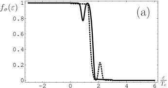
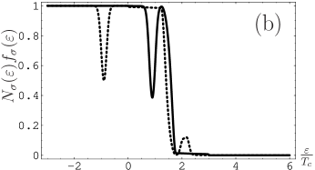
Figure 4: (a) The qualitative behavior of the distribution function $f_{\sigma}(\varepsilon)$ in the interlayer in dependence on $\varepsilon$. Solid and dashed lines are related to spin-up and spin-down electrons, respectively. (b) A typical behavior of the product $N_{\sigma}(\varepsilon)f_{\sigma}(\varepsilon)$ as a function of the quasiparticle energy.

On the contrary, in the presence of the proximity induced features the product $N_{\sigma}(\varepsilon)f_{\sigma}(\varepsilon)$ is different for spin-up and spin-down electrons in the interval $[\varepsilon_{1},\varepsilon_{2}]$, as it is demonstrated in Fig. 4(b), what leads to the discussed above constant limiting behavior of the dc spin current. The limiting constant behavior of the ac current also originates from this term. The point is that the particular shape (especially width) of the minigap features is fairly sensitive to the phase difference at SFS junction. As in the nonequlibrium conditions the phase difference is driven by the factor $2eVt$, all the features generated by the minigap in Fig. 4 oscillate in time with the corresponding frequency, giving rise to ac contribution to the current.

Another interesting property of the ac current flowing through the probe electrode is the possibility to obtain coherent highly spin-polarized ac currents with a certain phase shift between them. The point is that the values of the Green’s functions $\hat{g}^{R,A,K}_{F}$ in the interlayer, which determine the current flowing through the probe electrode, depend on the coordinate $x$ across SFS junction. At the same time the frequency of their oscillating part is position-independent and controlled by the voltage $V$ applied to SFS junction. Therefore, by coupling two probe electrode to different locations in the interlayer one can implement a source of coherent ac currents having a certain phase difference between them. Fig. 5 demonstrates the distribution of the ac electric current phases flowing through the probe electrode in our system in dependence of the coordinate $x$ across the interlayer (vertical axis) and the potential of the probe electrode $V_{p}$ (horizontal axis). The phase of the ac current is calculated with respect to the phase of the ac electric current, flowing through the SFS junction itself, because this reference value is independent on $V_{p}$ and location in the interlayer.

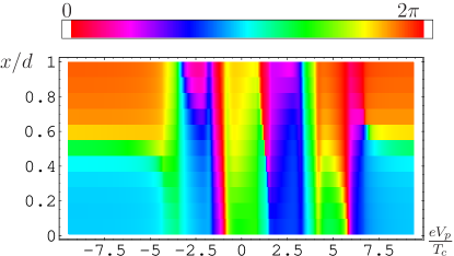
Figure 5: The distribution of the ac electric current phases flowing through the probe electrode in dependence of the coordinate $x$ across the interlayer (vertical axis) and the potential of the probe electrode $V_{p}$ (horizontal axis).

It is seen in Fig. 5 that the phase shift close to $\pi$ can be obtained for a wide $V_{p}$ range by coupling the probe electrodes symmetrically with respect to the middle of the junction. In principle, phase shifts close to $\pi/2$ are also reachable, although for a narrower ranges of $V_{p}$, as it is seen in Fig. 5.

The most part of the discussed above results is pronounced in the regime, when the value of the exchange field $h$ (measured in the energy units) is of order of superconducting order parameter $\Delta$. In ferromagnetic alloys like $CuNi$, which have been intensively used by now for experimental investigation of equilibrium properties of SFS heterostructures, the exchange field is several times larger than $\Delta$. However, as far as we know, the work on the creation of appropriate alloys is in progress now, so we believe that this limit can be experimentally realized in the nearest future. As the F layer is supposed to be an alloy, a role of magnetic scattering may be quite importantSellier03 ; Ryazanov04 . Therefore, the influence of the magnetic scattering on the results, obtained in this paper should be also investigated.

In conclusion, in the paper we have theoretically obtained that voltage-biased SFS junction in the regime of the essential proximity effect can be used as a source of highly spin-polarized ac current by tunnel coupling the interlayer region to the additional normal electrode. This current is driven by the non-equilibrium proximity effect in the system and vanishes if the proximity features are suppressed somehow. The frequency of the ac current is controlled by the voltage $V$ applied to SFS junction. In addition this system can implement a source of coherent ac currents having a certain phase difference between them by coupling two probe electrode to different locations in the interlayer.

Acknowledgments The support by the Russian Science Support Foundation (A.M.B.), RF Presidential Grant No.MK-4605.2007.2 (I.V.B.) and the programs of Physical Science Division of RAS are acknowledged.

References

- (1) A.I. Buzdin, Rev.Mod.Phys. 77, 935 (2005).
- (2) M. Eschrig, J. Kopu, J.C. Cuevas, and G. Schön, Phys.Rev.Lett. 90, 137003 (2003).
- (3) R.S. Keizer, S.T.B. Goennenwein, T.M. Klapwijk, G. Miao, G. Xiao, and A. Gupta, Nature 439, 825 (2006).
- (4) S. Takahashi, H. Imamura, and S. Maekawa, Phys. Rev. Lett. 82, 3911 (1999).
- (5) S. Maekawa, S. Takahashi, and H. Imamura, J. Phys. D: Appl. Phys. 35, 2452 (2002).
- (6) Y. Tserkovnyak and A. Brataas, Phys. Rev. B 65, 094517 (2002).
- (7) J. Johansson, V. Korevinski, D.V. Haviland, and A. Brataas, Phys. Rev. Lett. 93, 216805 (2004).
- (8) V. Pena, Z. Sefrioui, D. Arias, C. Leon, J. Santamaria, J.L. Martinez, S.G.E. te Velthuis, and A. Hoffmann, Phys. Rev. Lett. 94, 057002 (2005).
- (9) J.P. Morten, A. Brataas, and W. Belzig, Phys. Rev. B 72, 014510 (2005).
- (10) W. Belzig, A. Brataas, Yu.V. Nazarov, and G.E.W. Bauer, Phys. Rev. B 62, 9726 (2000).
- (11) S. Takahashi, T. Yamashita, T. Koyama, and S. Maekawa, J. Appl. Phys. 89, 7505, (2001).
- (12) J.P. Morten, A. Brataas, and W. Belzig, Phys. Rev. B 70, 212508 (2004).
- (13) F. Giazotto, F. Taddei, R. Fazio, and F. Beltram, Phys. Rev. Lett. 95, 066804 (2005).
- (14) F. Giazotto, F. Taddei, P. D’Amico, R. Fazio, and F. Beltram, Phys. Rev. B 76, 184518 (2007).
- (15) F. Giazotto and F. Taddei, Phys. Rev. B 77, 132501 (2008).
- (16) D. Huertas-Hernando, Yu.V. Nazarov, and W. Belzig, Phys. Rev. Lett. 88, 047003 (2002).
- (17) I.V. Bobkova and A.M. Bobkov, Phys. Rev. B 74, R220504 (2006).
- (18) S. Hikino, M. Mori, S. Takahashi, and S. Maekawa, arxiv:0809.1470.
- (19) W.L. McMillan, Phys. Rev. 175, 537 (1968).
- (20) R. Fazio and C. Lucheroni, Europhys. Lett. 45, 707 (1999).
- (21) K.D. Usadel, Phys.Rev.Lett. 25, 507 (1970).
- (22) M. Eschrig, Phys. Rev. B 61, 9061 (2000).
- (23) M. Eschrig, J. Kopu, A. Konstandin, J.C. Cuevas, M. Fogelström, and Gerd Schön, Advances in Solid State Physics, 44, 533 (2004).
- (24) M.Yu. Kupriyanov and V.F. Lukichev, Sov. Phys. JETP 67, 1163 (1988).
- (25) A. Millis, D. Rainer, and J. A. Sauls, Phys. Rev. B 38, 4504 (1988).
- (26) H. Sellier, C. Baraduc, F. Lefloch, and R. Calemczuk, Phys.Rev. B 68, 054531 (2003).
- (27) V.V. Ryazanov, V.A. Oboznov, A.S. Prokofiev, V.V. Bolginov, A.K. Feofanov, Journ. Low Temp. Phys. 136, 385 (2004).