Apparent violation of equipartition of energy in constrained dynamical systems

Abstract

We propose a planar chain system, which is a simple mechanical system with a constraint. It is composed of $N$ masses connected by $N-1$ light links. It can be considered as a model of a chain system, e.g., a polymer, in which each bond is replaced by a rigid link. The long time average of the kinetic energies of the masses in this model is numerically computed. It is found that the average kinetic energies of the masses are different and masses near the ends of the chain have large energies. We explain that this result is not in contradiction with the principle of equipartition. The apparent violation of equipartition is observed not only in the planar chain systems but also in other constrained systems. We derive an approximate expression for the average kinetic energy, which is in qualitative agreement with the numerical results.

Information on energy distribution in many-body systems is quite important for both theoretical and practical purposes. If a system is in thermal equilibrium, then, according to the principle of equipartition of energy, the average kinetic energy is equally distributed among all the degrees of freedom. Even when this principle holds, however, we found that nonuniform distribution of the average kinetic energy can occur.

In this letter, we introduce a system called a “planar chain system”, which is a simplified model of a chain system e.g., a polymer. We show that the average kinetic energy in this system is nonuniformly distributed even when it is in thermal equilibrium, but the principle of equipartition is not violated. We explain the reason for the nonuniform distribution of energy, which we refer to as the “apparent violation of equipartition of energy”. This property of apparent violation of equipartition of energy could provide a new insight into the behavior of chain systems.

Figure 1: A planar chain system

Let us introduce the planar chain system. The planar chain system is composed of $N$ particles (masses) connected by $N-1$ links. The masses can rotate smoothly, as shown in Fig.1. The links are massless and have fixed lengths. The system is defined by the following Lagrangian $L$ and constraints $g_{i}$ ($i=1,2,\cdots,N-1$):

$$L =\sum_{i=1}^{N}\frac{m_{i}}{2}\left(\dot{x}_{i}^{2}+\dot{y}_{i}^{2}\right)-U(\left\{\overrightarrow{r_{i}}\right\})\ ,$$ (1)

$$g_{i}(\left\{\overrightarrow{r_{j}}\right\}) \equiv\frac{1}{2}\left\{\left|\overrightarrow{r_{i+1}}-\overrightarrow{r_{i}}\right|^{2}-\ell_{i}^{2}\right\}=0,$$ (2)

where $N$ is the number of particles, $m_{i}$ is the mass of $i$’th particle, $\overrightarrow{r_{i}}\equiv(x_{i},y_{i})$ represents the position of the $i$’th particle, and $\ell_{i}$ is the length of the $i$’th link. $U$ represents potential energy. We consider (i) a free chain with $U\equiv 0$ and (ii) external potential $U\equiv\sum_{i=1}^{N}V(\overrightarrow{r_{i}})$.

If we define $\varphi_{i}$ as the angle between the $i$’th link and the $-y$ direction (Fig.1), we can rewrite the Lagrangian without the constraint. First we consider the following relations: $x_{i+1}-x_{i}=\ell_{i}\sin\varphi_{i}$ ,  $y_{i+1}-y_{i}=-\ell_{i}\cos\varphi_{i}\ .$ Using the total mass $M$ and the center of mass $(X_{G},Y_{G})$ defined as $M\equiv\sum_{i=1}^{N}m_{i},$ $X_{G}\equiv\sum_{i=1}^{N}\frac{m_{i}}{M}x_{i},$  $Y_{G}\equiv\sum_{i=1}^{N}\frac{m_{i}}{M}y_{i},$ we obtain

$$x_{i}=X_{G}+\sum_{j=1}^{N-1}a_{ij}\sin\varphi_{j}\,,\ \ y_{i}=Y_{G}-\sum_{j=1}^{N-1}a_{ij}\cos\varphi_{j}\,,$$ (3)

where $a_{ij}$ is defined as

$$a_{ij}\equiv\begin{cases}\displaystyle\phantom{-}\mu_{j}^{\leq}\,\ell_{j}&\ :\ j<i\ ,\\ \displaystyle-\mu_{j}^{>}\,\ell_{j}&\ :\ j\geq i\ ,\\ \end{cases}$$ (4)

and

$$\mu_{k}\equiv\frac{m_{k}}{M},\ \ \mu_{n}^{\leq}\equiv\sum_{k=1}^{n}\mu_{k}\ ,\ \ \mu_{n}^{>}\equiv\sum_{k=n+1}^{N}\mu_{k}\ .$$ (5)

By a straightforward calculation, we obtain the Lagrangian (1) in terms of $\varphi_{i}$’s and $(X_{G},Y_{G})$ as

$$L =\frac{M}{2}(\dot{X}_{G}^{2}+\dot{Y}_{G}^{2})+\frac{M}{2}\!\sum_{j,k=1}^{N-1}A_{jk}(\varphi)\dot{\varphi}_{j}\dot{\varphi}_{k}$$

$$-U(X_{G},Y_{G},\left\{\varphi_{i}\right\})\ \ ,$$ (6)

$$A_{jk}(\varphi) \equiv\mu_{\min(j,k)}^{\leq}\,\mu_{\max(j,k)}^{>}\,\cos(\varphi_{jk})\ell_{j}\ell_{k}\ ,$$ (7)

where $\varphi_{jk}\equiv\varphi_{j}-\varphi_{k}$.

We can consider this system as a simplified prototype of various chain systems, e.g., proteins, polymers and spacecraft manipulators, under the assumption that the frequencies of bond-stretching vibrations are quite high.

Now, we describe a method for numerical simulation. The Lagrangian that is expressed in terms of angles (6) is complicated and it is difficult to numerically integrate the equation of motion, in particular for large $N$. Hence, we use the original form of the Lagrangian (1) and the constraint $g_{i}$ (2). Then, the equation of motion includes terms of the constraint, which is called a “Lagrange multiplier” Goldstein (1980). We determine Lagrange multipliers numerically at each integration step so that the constraint is satisfied Leimkuhler and Reich (2004). Methods of this type, e.g., “SHAKE” and “RATTLE” algorithms, are widely used for molecular simulation in chemistry  Ryckaert et al. (1977); Barth et al. (1995); http://www.charmm.org/ . In addition, some of the algorithms are known to be symplectic Leimkuhler and Reich (2004). Here, we use the forth-order symplectic integrator. In some cases, we verify the results by using an implicit Runge-Kutta method.

If $U\equiv 0$, the total angular momentum is conserved, hence, in this case, the energy distribution is different from the microcanonical distribution. In actual computations, we place the system in a potential wall composed of arcs of radius $a$: $U\equiv\sum_{i=1}^{N}V(\overrightarrow{r_{i}})$, $V(\overrightarrow{r})=0.01\sum_{j=1}^{N_{\text{wall}}}\left|\left|\overrightarrow{r}-\overrightarrow{R}_{\text{j}}\right|-a\right|^{-6}$. Then, the system exhibits strongly chaotic motion similar to billiards Chernov and Markarian (2006) and does not have any conserved quantities other than the total energy, hence the microcanonical distribution is restored.

Figure 2: Planar chain in potential wall. $N=5$, $N_{\text{wall}}=4$, $a=4N\ell$, $R_{j}=(R,0),(-R,0),(0,R),(0,-R)$, $R=N\ell+\sqrt{a^{2}-N^{2}\ell^{2}}$. $\ell_{1}=\cdots=\ell_{N-1}\equiv\ell$.

Although the planar chain system is a simple system, its dynamics is complex; further, energy exchanges occur between various parts of the system. Fig. 3 shows a power spectrum of $x_{1}(t)$ with the external potential mentioned above. It is a broad continuous spectrum, which is a manifestation of chaotic motion Lichtenberg and Lieberman (1992).

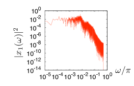
Figure 3: Power spectrum of $x_{1}(t)$ for $0\leq t\leq 32767$. $N=5$. External potential in Fig.2 is used to obtain the spectrum.

Using the method described above, we compute the long time average of kinetic energy. If the averaging time is sufficiently large, the long time average and thermal average can be assumed to be the same.

The kinetic energy of $i$’th particle is defined as $K_{i}(t)\equiv\frac{m_{i}}{2}\left(\dot{x}_{i}^{2}+\dot{y}_{i}^{2}\right)\,,$ and its long time average is defined as

$$\overline{K_{i}}\equiv\frac{1}{t_{\text{max}}}\int_{0}^{t_{\text{max}}}K_{i}(t)\,dt\ ,\ t_{\text{max}}\rightarrow\infty\ .$$ (8)

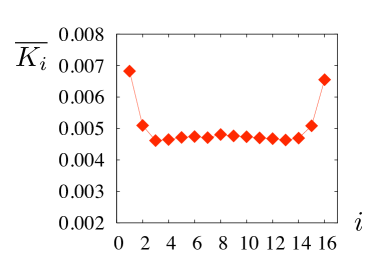
Figure 4: Long time average of kinetic energy $\overline{K_{i}}$ vs. $i$ (8). $N=16$. $m_{i}=1.0$ for all $i$ and  $\ell_{i}=1.0$ for all $i$. The initial condition is as follows: $x_{i}=(i-1)-N/2$, $y_{i}=0$, $p^{(x)}_{i}=0$ for all $i$, $p^{(y)}_{1}=-0.1$, and $p^{(y)}_{i}=0.1(i>1)$. Here, $p^{(x)}_{i}$ and $p^{(y)}_{i}$ represent the $x$ and $y$ components of the momentum of the $i$’th particle, respectively. The time step for integration is $dt=0.001$. $t_{\text{max}}$ (8) is $10^{5}$. The relative error for total energy (square root of the time average of the squared displacement) is $\sqrt{\overline{\Delta E^{2}/E_{0}^{2}}}=6.1\times 10^{-11}$.

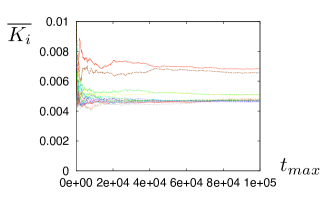
Figure 5: Convergence of kinetic energy $K_{i}$ (8) in Fig.4 as a function of $t_{\text{max}}$.

One might think that the values of all $\overline{K_{i}}$’s in this system must be the same, by regarding $K_{i}$ as the kinetic energy of the $i$-th degree of freedom and applying the principle of equipartition of energy. However, this is not true. Fig.4 shows a plot of the average kinetic energy of each mass $\overline{K_{i}}$ (8) against $i$ for $N=16$ planar chain system. It is clear that the $\overline{K_{i}}$’s are not equally distributed. More importantly, we find that masses that are near the ends of the chain have large kinetic energies. We obtain this result for all the computed system sizes ( $N\leq 64$ ). Fig. 5 shows the convergence of $\frac{1}{t_{\text{max}}}\int_{0}^{t_{\text{max}}}K_{i}(t^{\prime})dt^{\prime}$ as a function of $t_{\text{max}}$. The values shown in Fig.4 are well converged.

However, this remarkable result is not in contradiction with the principle of equipartition of energy. The principle of equipartition of energy is stated as follows Kubo et al. (1990): Suppose we have a system defined by a Hamiltonian

$$H(q,p)\equiv K(q,p)+V(q),\ K(q,p)\equiv\sum_{i,j=1}^{\mathcal{N}}\frac{1}{2}\alpha_{ij}(q)p_{i}p_{j}\ \ ,$$ (9)

where $p_{i}$ and $q_{i}$ are canonically conjugate to each other and $\mathcal{N}$ is the total number of degrees of freedom. If it is in thermal equilibrium at temperature $T$, then the following relation holds:

$$\left<\frac{1}{2}p_{i}\displaystyle\frac{\partial K}{\partial p_{i}}\right>=\frac{1}{2}k_{B}T$$ (10)

(Summation over the index $i$ is not taken in the left hand side.). The symbol $\left<\cdots\right>$ represents thermal average at $T$, and is defined as

$$\left<f(q,p)\right>\equiv\frac{1}{Z}\int f(q,p)e^{-\beta H}d\Gamma\ ,$$ (11)

for any function $f(q,p)$. Here, $d\Gamma$ is a volume element of phase space, $Z$ is a partition function, and $\beta\equiv 1/k_{B}T$.

Let us define the “canonical kinetic energy” $K_{i}^{(c)}$ and the “linear kinetic energy” $K_{i}$ as

$$K_{i}^{(c)}\equiv\frac{1}{2}p_{i}\displaystyle\frac{\partial K}{\partial p_{i}},\ \ \ \ K_{i}\equiv\frac{1}{2}m_{i}v_{i}^{2},$$ (12)

respectively. Here, equipartition of energy means that the average values of $K_{i}^{(c)}$’s are equal at thermal equilibrium.

For systems such as gas models or lattice models, $\alpha_{ij}(q)=m_{i}^{-1}\delta_{ij}$ and $K_{i}^{(c)}=K_{i}$: hence, the principle of equipartition (10) simply means that $\left<\frac{1}{2}m_{i}v_{i}^{2}\right>=\frac{1}{2}k_{B}T\ ,$ which is a commonly used form of equipartition of energy.

However, in the case of a planar chain system, equipartition of energy has a different meaning. From  (6), we obtain the canonical momentum $p_{i}$ that is conjugate to $\varphi_{i}$ as $p_{i}\equiv\frac{\partial L}{\partial\dot{\varphi}_{i}}=\sum_{k=1}^{N-1}A_{ik}(\varphi)\dot{\varphi}_{k}\ ,$ and we obtain the canonical kinetic energy $K_{i}^{(c)}$ for the planar chain system as

$$K_{i}^{(c)}\equiv\frac{1}{2}p_{i}\displaystyle\frac{\partial K}{\partial p_{i}}=\frac{1}{2}\sum_{k=1}^{N-1}A_{ik}(\varphi)\dot{\varphi}_{k}\dot{\varphi}_{i}\ .$$ (13)

For example, eq. (13) with $N=3$ and $i=1$ we have

$$K_{1}^{(c)}=\frac{M}{2}\left\{\mu_{1}(\mu_{2}+\mu_{3})\ell_{1}^{2}\dot{\varphi}_{1}^{2}+\mu_{1}\mu_{3}\ell_{1}\ell_{2}\dot{\varphi}_{1}\dot{\varphi}_{2}\cos\varphi_{12}\right\}\ .$$ (14)

It should be noted that $K_{i}^{(c)}$ is defined by variables of every part of the system, whereas $K_{i}$ is defined only by the $i$-th particle. In other words, canonical kinetic energy $K_{i}^{(c)}$ is extended, whereas linear kinetic energy $K_{i}$ is localized. Hence it is obvious that $K_{i}^{(c)}\neq K_{i}$. Since $K_{i}^{(c)}$ obeys equipartition of energy, we can consider that $K_{i}$ does not obey this principle.

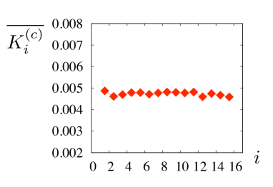
Figure 6: Long time average of canonical kinetic energy $\overline{K_{i}^{(c)}}$ (13) vs $i$. This plot is obtained by using the same data as that in Fig.4.

Fig. 6 shows the long time average of $K_{i}^{c}$ (13) for the same time series as that in Fig. 4. It is clearly shown that $\overline{K_{i}^{(c)}}$ ’s take almost the same value for all $i$. That is, equipartition of energy is realized. Non-equipartition of energy clearly shown in Fig.4 does not imply that principle of equipartition is violated. In other words, although the system obeys the principle of equipartition of energy, the values of the linear kinetic energy are different at different points in the system. We refer to the variation in $\left<K_{i}\right>$ under thermal equilibrium as the “apparent violation of equipartition of energy”.

We derive the nonuniformity of the energy distribution by analytical calculation. By a straightforward calculation, we obtain

$$\frac{\left<K_{i}\right>}{k_{B}T} =\frac{m_{i}}{M}+\frac{m_{i}}{2k_{B}T}\sum_{j,k=1}^{N-1}a_{ij}a_{ik}\left<\cos\left(\varphi_{jk}\right)\dot{\varphi}_{j}\dot{\varphi}_{k}\right>\ .$$ (15)

To evaluate the second term, we adopt the following approximations:

$$\left<\cos\left(\varphi_{jk}\right)\dot{\varphi}_{j}\dot{\varphi}_{k}\right>=0\ \ \text{for}\ j\neq k\ ,$$ (16)

$$\left(A^{-1}\right)_{jj}\sim\frac{1}{A_{jj}}=\frac{1}{M\mu_{j}^{\leq}\mu_{j}^{>}\ell_{j}^{2}}\ \ .$$ (17)

(The matrix $A^{-1}$ is included in $\exp(-\beta H)$.) These approximations indicate that each link in the chain rotates independently. Then, we obtain

$$\frac{\left<K_{i}\right>}{k_{B}T}=\frac{m_{i}}{M}\left\{1+\frac{1}{2}\left[\sum_{j=1}^{i-1}\left(\frac{\mu_{j}^{\leq}}{\mu_{j}^{>}}\right)+\sum_{j=i}^{N-1}\left(\frac{\mu_{j}^{>}}{\mu_{j}^{\leq}}\right)\right]\right\}\,.$$ (18)

Details of the calculation will be shown elsewhere Konishi and Yanagita (a).

Eq.(18) shows that the average linear kinetic energy $\left<K_{i}\right>$ varies from point to point. In other words, “apparent violation of equipartition of energy” occurs in this system.

If all the masses are the same $m_{i}=m,$ then we obtain

$$\frac{\left<K_{i}\right>}{k_{B}T}=\frac{1}{N}\left\{1+\frac{1}{2}\left[\sum_{j=1}^{i-1}\left(\frac{j}{N-j}\right)+\sum_{j=i}^{N-1}\left(\frac{N-j}{j}\right)\right]\right\}\,.$$ (19)

This expression implies the following:

$$\langle K_{1}\rangle>\langle K_{2}\rangle>\cdots<\langle K_{N-1}\rangle<\langle K_{N}\rangle\ .$$ (20)

It is clear that $\langle K_{i}\rangle$ is large at the ends of the chain and small at the center of the the chain: this result is in qualitative agreement with the result of the numerical computation shown in Fig.4.

In this letter we have numerically shown that $\displaystyle K_{i}\equiv\frac{m_{i}}{2}v_{i}^{2}$ does not obey the principle of equipartition of energy for the planar chain system. Moreover $\overline{K_{i}}$ of particles that are near both ends of the chain is large. The nonuniform distribution of the linear kinetic energy is qualitatively explained by analytical calculation.

The apparent contradiction is due to the difference between $K_{i}\equiv\frac{1}{2}m_{i}v_{i}^{2}$ and $K_{i}^{c}\equiv\frac{1}{2}p_{i}\displaystyle\frac{\partial K}{\partial p_{i}}$. This difference is caused by the presence of the coordinate $q$ ($\varphi$ for planar chain systems) in the expression of the kinetic energy $K$, due to the existence of the constraint. Further, the same numerical time series show that the average values of $K_{i}^{(c)}$ are equal, i.e., the system obeys the principle of equipartition.

It is clear that there are other models in which the values of the average kinetic energy are not equal. These models are systems with constraints, where the expression of the kinetic energy includes coordinates. In fact, it has been found that the behavior of linear kinetic energy in a multiple pendulum system is similar to that in the planar chain system  Oyama and Yanagita (1998); and we will report detailed analysis elsewhere Konishi and Yanagita (b). In polymer science, the three-dimensional version of this model is known as a “freely jointed chain” Kramers (1946); Mazars (1996). We expect that the behavior of the kinetic energy in the freely jointed chain will be similar to that in the planar chain system.

We have shown that in the planar chain system, the energy at the ends of the chain is larger than that at the center. This result may be considered rather trivial, because it may seem that the end parts can be moved easily. However, even in thermal equilibrium, where all degrees of freedom have the same energy on average, the energy at the ends of the chain is large.

This result would have important implications for the dynamics of chain systems such as molecules, proteins, polymers, and some artificial objects. For example, in polymer science, it is well known that atoms situated near the ends of the polymer chain have characteristic behavior called the “end effect” Tokita et al. (2004). Apparent violation of equipartition of energy we found in planar chain systems can be closely related to the origin of the end effect of polymers.