Phase diagram of the non-uniform chiral condensate in different regularization schemes at T=0

Abstract

We show that the qualitative picture of the phase diagram which includes the non-uniform chiral phase and 2SC superconducting phase is independent of the considered regularization schemes. We also demonstrate that the quantitative results agree with each other reasonably for the set of so called "relativistic" regularization schemes. On the other hand the "non-relativistic" momentum cut-off is clearly differ from the others.

I Introduction

The phase diagram of strongly interacting matter is in the center of scientific interest for many decades. During the last decade there was a great progress in our understanding of this subject which was based on the simple observation that Cooper instability and asymptotic freedom jointly lead to the colour superconductivity phenomenon at asymptotically high densities shuryak_alford_son . However, at moderate densities our knowledge is still limited to the model dependent calculations. A variety of phases are possible which is a direct consequence of the richness of strong (and indirectly weak) interactions between elementary constituents of matter. In particular, the high symmetry groups involved in the description allow the existence of many different types of phases. Of special interest are non-uniform phases. Among those, the LOFF phases of superconductivity loff_alford , Overhauser effect over or non-uniform chiral condensates dautry_bron_sad_jap are very good examples.

In this paper, we ask the technical but important question of the regularization dependence of the phase diagram of strongly interacting matter which contains the non-uniform chiral condensate. This drawback is inferred by the fact that the NJL model describing strong interactions is an effective non-renormalizable approximation. Then different regularization schemes lead, in a sense, to different models. It is important to check if qualitative results are independent of the regularization scheme, and what is their dependence at the quantitative level.

We consider the phase diagram at finite density which includes chiral uniform and non-uniform phases, superconducting 2SC phase and plasma of the free quarks sad . Herein we checked the phase diagram within the Nambu - Jona-Lasinio model against four various schemes, namely 3- and 4-dim cut-off, Schwinger and Pauli-Villars regularization. Similar analysis was performed in the case of single non-uniform chiral phase in bron_kutsch . As the main result we confirm that the non-uniform phase exists in all considered regularization schemes.

We expect that the most important differences emerge at zero temperature thus we consider only this situation. At higher temperature, the major role would be played by the finite temperature corrections. However, inclusion of those is outside the scope of our paper.

II Model

The starting point is based on the Nambu - Jona-Lasinio model with two flavours sad1

$$H=\int_{x}\left\{\bar{\psi}(i\gamma^{\nu}\partial_{\nu}+\mu\gamma_{0})\psi+G\left[(\bar{\psi}\psi)^{2}+(\bar{\psi}i\gamma_{5}\vec{\tau}\psi)^{2}\right]+G^{\prime}(\bar{\psi}_{c}i\gamma_{5}\tau_{2}\lambda^{A}\psi)(\bar{\psi}i\gamma_{5}\tau_{2}\lambda^{A}\psi_{c})\right\}$$ (1)

where $\psi$ is the quark field, $\psi_{c}=C\bar{\psi}^{T}$ is the conjugate field and $\mu$ is the quark chemical potential. The color, flavor and spinor indices are suppressed. The vector $\vec{\tau}$ is the isospin vector of Pauli matrices and $\lambda^{A}$, $A=2,5,7$ are three color antisymmetric $SU(3)$ group generators. The integration $\int_{x}=\int_{0}^{\beta}d\tau\int d^{3}x$, where $\beta$ is the inverse temperature and derivative operator $\partial_{\nu}=(i\partial_{\tau},\vec{\nabla})$. Two coupling constants $G,G^{\prime}$ describe interactions which are responsible for the creation of quark-antiquark and quark-quark condensates respectively. Both couplings are treated as independent. There is also an additional parameter $\Lambda$ which defines the energy scale below which the effective theory applies. It is introduced through the regularization procedure.

We are working in the mean field approximation within the ansatz sad1

$$\langle\bar{\psi}\psi\rangle=-\frac{M}{2G}\cos\vec{q}\cdot\vec{x},\;\;\;\langle\bar{\psi}i\gamma_{5}\tau^{a}\psi\rangle=-\frac{M}{2G}\delta_{a3}\sin\vec{q}\cdot\vec{x},\;\;\;\langle\psi\tau_{2}\lambda^{A}C\gamma_{5}\psi\rangle=\frac{\Delta}{2G^{\prime}}\delta_{A2}$$ (2)

which describes three possible phases: the chiral uniform phase ($\vec{q}=0,M\neq 0,\Delta=0$), the non-uniform chiral phase ($\vec{q}\neq 0,M\neq 0,\Delta=0$) and the superconducting phase ($\vec{q}=0,M=0,\Delta\neq 0$). All mentioned phases can coexist with each other. Using standard methods one can calculate the thermodynamic potential sad ; sad1

$$\Omega_{0}=\frac{M^{2}}{4G}+\frac{|\Delta|^{2}}{4G^{\prime}}+2\sum_{s=\pm}\int_{E_{s}\leq\mu}\frac{d^{3}k}{(2\pi)^{3}}(E_{s}-\mu)-2\sum_{s=\pm}\int\frac{d^{3}k}{(2\pi)^{3}}\left(E_{s}+\sum_{i=\pm}E^{\Delta}_{i,s}\right),$$

$$E^{\Delta}_{\pm,s}=\sqrt{(\mu\pm E_{s})^{2}+|\Delta|^{2}},\;\;E_{\pm}=\sqrt{\vec{k}^{2}+M^{2}+\frac{\vec{q}^{\,2}}{4}\pm\sqrt{(\vec{q}\cdot\vec{k})^{2}+M^{2}\vec{q}^{\,2}}}$$ (3)

where the limit of zero temperature was already performed. The last integral is divergent. Before we introduce different regularization schemes let us convert equation (II) into another form which much better suits our purposes and better underlines the physics of the problem. To reach our goal we translate equation (II) into another form

$$\Omega = \frac{M^{2}}{4G}+\frac{|\Delta|^{2}}{4G^{\prime}}-2\sum_{s=\pm}\int\frac{d^{3}k}{(2\pi)^{3}}\left(\sum_{i=\pm}E^{\Delta}_{i,s}-2E_{s}\right)+4\sum_{i=\pm}\int\frac{d^{3}k}{(2\pi)^{3}}\left(E^{\Delta}_{i,0}-E^{\Delta=0}_{i,0}\right)$$

$$+ 2\sum_{s=\pm}\int_{E_{s}\leq\mu}\frac{d^{3}k}{(2\pi)^{3}}(E_{s}-\mu)-4\sum_{i=\pm}\int\frac{d^{3}k}{(2\pi)^{3}}\left(E^{\Delta}_{i,0}-E^{\Delta=0}_{i,0}\right)-6\sum_{s=\pm}\int\frac{d^{3}k}{(2\pi)^{3}}E_{s},$$

$$E^{\Delta}_{\pm,0} = \sqrt{(\mu\pm E_{0})^{2}+|\Delta|^{2}},\;\;E_{0}=\sqrt{\vec{k}^{2}+M^{2}}.$$ (4)

The first three integrals give finite contributions and only the last two are divergent. Let us note that in the absence of superconducting state the next to the last term vanishes and the only divergent contribution follows from the infinite Dirac sea integral. Additionally the last two integrals are separately dependent, the first one on $\Delta$ and the other one on wave vector $\vec{q}$. This separation is very convenient for the regularization procedure.

III Regularization schemes and parameters

In the first step we expand the last term of equation (II) in powers of the wave vector $\vec{q}$. It is well known that the parameter at the second order is related to the pion decay constant dautry_bron_sad_jap

$$-6\sum_{s=\pm}\int\frac{d^{3}k}{(2\pi)^{3}}E_{s}\approx-12\int\frac{d^{3}k}{(2\pi)^{3}}E_{0}+\frac{M^{2}f^{2}_{\pi}\vec{q}^{\,2}}{2M^{2}_{0}}.$$ (5)

where $M_{0}$ is constituent quark mass at zero density. The formula for the pion decay constant depends on the regularization and is known from the earlier literature (e.g. klev ). This formula together with expressions for the chiral condensate fixes the value of $G$ and $\Lambda$ parameters (Table 1). More details are discussed in the Appendix A. The coupling constant $G^{\prime}$ cannot be related to any known physical quantity. In the vast literature of color supercoductivity, its value is emplaced somewhere between $G/2\lesssim G^{\prime}\lesssim 3G/2$.

	3D	4D	S	PV
$\Lambda\;\;\;$	0.635	1.015	1.086	1.12
$G\Lambda^{2}\;\;\;$	2.2	3.93	3.78	4.47
$M_{0}\;\;\;$	0.33	0.238	0.2	0.22

Table 1: Numerical values of the regularization parameter $\Lambda$ in GeV and dimensionless quantity $G\Lambda^{2}$ for different regularization schemes. In the last row, the value of the quark constituent mass at zero density $M_{0}$ is given in GeV.

Taking into account equation (5) one can extract the divergent part of thermodynamic potential (II) in the form

$$\Omega_{div}=-4\sum_{i=\pm}\int\frac{d^{3}k}{(2\pi)^{3}}\left(E^{\Delta}_{i,0}-E^{\Delta=0}_{i,0}\right)-12\int\frac{d^{3}k}{(2\pi)^{3}}E_{0}.$$ (6)

We consider four types of different regularization schemes klev :

• 3-dim cut-off (3D) $\Lambda$ restricts the value of three dimensional momentum. The regularized potential takes the form

  $$\Omega^{3D}_{div}=-4\sum_{i=\pm}\int^{\Lambda}\frac{d^{3}k}{(2\pi)^{3}}\left(E^{\Delta}_{i,0}-E^{\Delta=0}_{i,0}\right)-12\int^{\Lambda}\frac{d^{3}k}{(2\pi)^{3}}E_{0}.$$ (7)

  This regularization was frequently used in previous papers e.g. sad .

• 4-dim cut-off (4D) restricts the value of four-momentum vector in Euclidean space. Using the formulae

  $$\int\frac{d^{3}k}{(2\pi)^{3}}(A-B)=\int\frac{d^{4}k_{E}}{(2\pi)^{4}}\ln\frac{k_{0}^{2}+A^{2}}{k_{0}^{2}+B^{2}}$$

  we introduce the cut-off parameter to the thermodynamic potential through the equation

  $$\Omega^{4D}_{div}=-8\int^{\Lambda}\frac{d^{4}k_{E}}{(2\pi)^{4}}\ln\frac{k_{0}^{2}+\frac{1}{4}(\sum_{i=\pm}E^{\Delta}_{i,0})^{2}}{k_{0}^{2}+\frac{1}{4}(\sum_{i=\pm}E^{\Delta=0}_{i,0})^{2}}-12\int^{\Lambda}\frac{d^{4}k_{E}}{(2\pi)^{4}}\ln(k_{0}^{2}+E_{0}^{2}),$$ (8)

  where $d^{4}k_{E}=dk_{0}d^{3}k$.

• Schwinger regularization (S) is based on the formula

  $$\ln\frac{A}{B}=\int_{0}^{\infty}\frac{d\tau}{\tau}[\exp(\tau(B+i\epsilon))-\exp(\tau(A+i\epsilon))].$$

  This leads us to the regularized expression for the potential

  $$\Omega^{S}_{div} = -8\int\frac{d^{4}k_{E}}{(2\pi)^{4}}\int_{1/\Lambda^{2}}^{\infty}\frac{d\tau}{\tau}\left\{\exp\left[\tau\left(-k_{0}^{2}-\frac{1}{4}(\sum_{i=\pm}E^{\Delta}_{i,0})^{2}\right)\right]\right.$$ (9)

  $$- \left.\exp\left[\tau\left(-k_{0}^{2}-\frac{1}{4}(\sum_{i=\pm}E^{\Delta=0}_{i,0})^{2}\right)\right]\right\}$$

  $$- 12\int\frac{d^{4}k_{E}}{(2\pi)^{4}}\int_{1/\Lambda^{2}}^{\infty}\frac{d\tau}{\tau}\left\{\exp\left[\tau\left(-k_{0}^{2}-E_{0}^{2}\right)\right]\right\}.$$

  This regularization was considered in nakano where only the single non-uniform chiral phase was taken into account.

• Pauli-Villars regularization (PV) introduces an arbitrary number of coupling constants $C_{a}$ and mass regulators $M_{a}$ combine in such a way that divergent potential (6) becomes finite. In the first step we regularized potential by the 3-dim cut-off and then expand the result around the large value of the parameter $\Lambda$. The values of coupling constants $C_{a},M_{a}$ are already set by the conditions which follows from the calculation of the chiral condensate $\langle\bar{\psi}\psi\rangle$ and pion decay constant (the appendix). Then final expression for the thermodynamic potential in this scheme reads

  $$\Omega^{PV}_{div} = \frac{3}{8\pi^{2}}\sum_{\alpha=1}^{3}C_{\alpha}M^{4}_{\alpha}\ln\frac{M^{2}}{M_{\alpha}^{2}}+\frac{1}{\pi^{2}}\left(\frac{|\Delta|^{4}}{4}-|\Delta|^{2}\mu^{2}\right)\sum_{\alpha=1}^{3}C_{\alpha}\ln\frac{M^{2}+|\Delta|^{2}}{M_{\alpha}^{2}+|\Delta|^{2}}$$ (10)

  $$+ \frac{|\Delta|^{2}}{2\pi^{2}}\sum_{\alpha=1}^{3}C_{\alpha}M_{\alpha}^{2}\ln\frac{M^{2}+|\Delta|^{2}}{M_{\alpha}^{2}+|\Delta|^{2}}+\frac{1}{4\pi^{2}}\sum_{\alpha=1}^{3}C_{\alpha}M_{\alpha}^{4}\left(\ln\frac{M^{2}+|\Delta|^{2}}{M_{\alpha}^{2}+|\Delta|^{2}}-\ln\frac{M^{2}}{M_{\alpha}^{2}}\right),$$

where $C_{a},M_{a}$ are given by equations (13) in the appendix.

IV Results

We minimize the thermodynamic potential

$$\Omega = \frac{M^{2}}{4G}+\frac{|\Delta|^{2}}{4G^{\prime}}+\frac{M^{2}F^{2}_{\pi}\vec{q}^{\,2}}{2M^{2}_{0}}-2\sum_{s=\pm}\int\frac{d^{3}k}{(2\pi)^{3}}\left(\sum_{i=\pm}E^{\Delta}_{i,s}-2E_{s}\right)+4\sum_{i=\pm}\int\frac{d^{3}k}{(2\pi)^{3}}\left(E^{\Delta}_{i,0}-E^{\Delta=0}_{i,0}\right)$$ (11)

$$+ 2\sum_{s=\pm}\int_{E_{s}\leq\mu}\frac{d^{3}k}{(2\pi)^{3}}(E_{s}-\mu)+\Omega^{scheme}_{div}$$

with respect to mass $M$, wave vector $\left|\vec{q}\right|$ and gap parameter $\Delta$ as a function of chemical potential. The last term of (11) depends on the scheme as was described in the previous section. Appropriate formule for $\Omega^{scheme}_{div}$ are given by equations (7, 8, 9, 10).

As already discussed $G,\Lambda$ coupling constants are determined by the values of the pion decay constant and the size of the chiral condensate at zero density (Table I). The remaining constant $G^{\prime}$ is essentially unknown. For the presentation of the result we assume $G^{\prime}=0.75G$ which follows from the Fierz transformation buballa . The choice of another ratio $G^{\prime}/G$ does not influence our analysis of the result dependence on regularization schemes. The values of constituent mass, wave vector and gap parameter as a function of chemical potential for different regularization schemes are given in figures 1 - 3. As can be seen in all regularization schemes, there is the same pattern of the phase transitions. From uniform to non-uniform chiral phase and then to superconducting phase, all transitions are first order and existence of non-uniform phase is then independent of the considered regularization schemes. However, the strengths of the transition depend on the regularization scheme. This is particularly visible in Fig. 3.

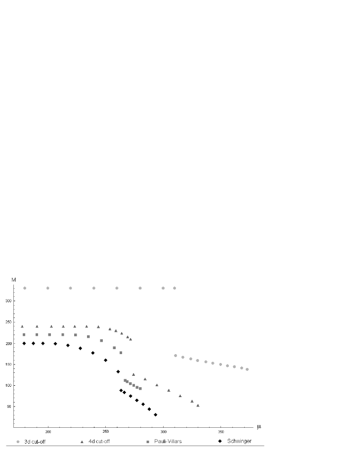
Figure 1: The constituent mass $M$ as a function of chemical potential $\mu$ in different regularization schemes in MeV units.

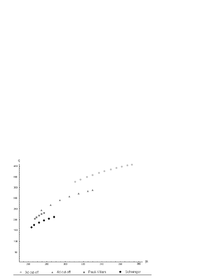
Figure 2: The value of the wave vector $q$ as a function of the chemical potential $\mu$ in the different regularization schemes in MeV units. The values of $\mu$ for non-zero $q$ describe the range of the existence of the non-uniform chiral phase.

Some quantitative features change with the chosen scheme. One can find that schemes cluster in two groups which one can call "relativistic" schemes (4D, S, PV) and 3D cut-off. However, let us note that the distinction between relativistic and non-relativistic schemes has no deep meaning because the thermodynamic system singles out one reference frame. Comparing the quantitative results, we consider values of constituent mass, wave vector, gap parameter, the strengths of the first order phase transitions and critical chemical potential. The position of the transition from uniform chiral to nonuniform chiral phase is the most resistant against the choice of the regularization scheme. First critical potential changes within the range of 5 per cent for relativistic schemes, while in the case of 3D within 18 per cent. The position of the second transition, for relativistic schemes changes within the range of 19 per cent, including 3D cut-off within 34 per cent. For 4D, S, PV schemes the range of variability of the parameter M value is about 20 per cent at $\mu$ equal to zero, and about 60 per cent at chemical potentials corresponding with first transition. The range of variability of parameter q value is 50 per cent at chemical potentials corresponding with first transition. Comparing M and q at second transition is unsuitable because of changeability of second critical potential. The dependence of the parameters M and q on the chemical potential is the same for the different regularizations. With increasing chemical potential, the value of q is growing, the M value is declining. Relatively the least correlated is the dependence of the parameter $\Delta$ on the regularization scheme. However, again the value of the gap $\Delta$ is increasing with $\mu$, independent of the regularization choice. The values of the critical chemical potentials of the phase transitions are given in Table II.

$\mu_{c}$	3D	4D	S	PV
Ch/NCH	0.311	0.274	0.263	0.268
NCH/2SC	0.373	0.330	0.296	0.281

Table 2: Numerical values of the critical chemical potentials $\mu_{c}$ in MeV for uniform and non-uniform chiral phase transition (Ch/NCH) and non-uniform chiral and superconducting phase transition (NCH/2SC) for different regularization schemes. In 3D, 4D, S schemes the 2SC phase appears already at Ch/NCh phase transition and both phases coexist. However, the value of the gap parameter is relatively low in the coexistence region. In the PV scheme, 2SC phase appears only at the NCh/2SC phase transition.

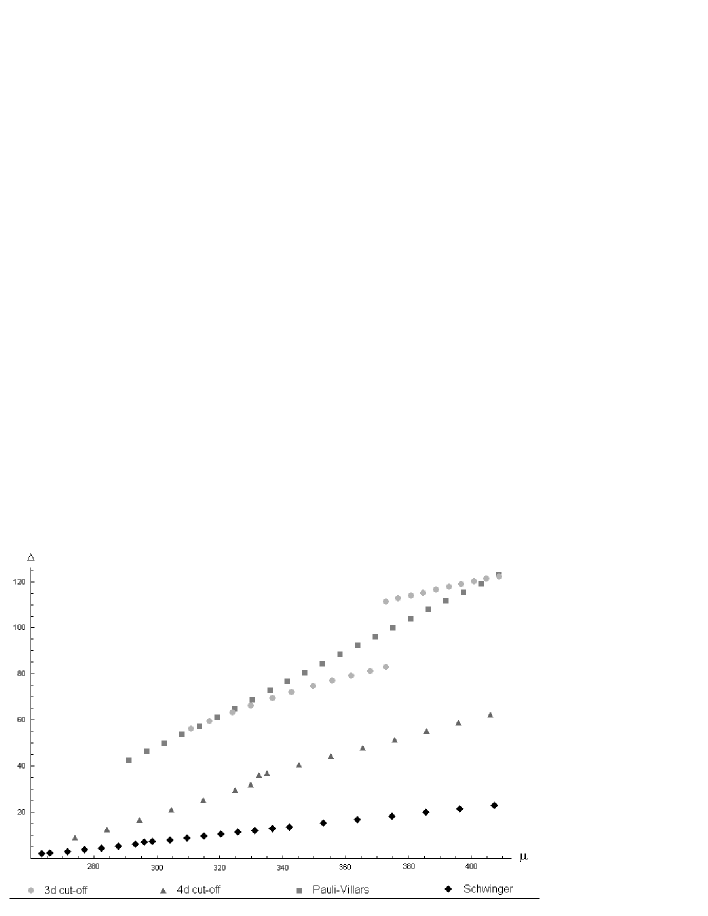
Figure 3: The gap parameter $\Delta$ as a function of chemical potential $\mu$ in different regularization schemes in MeV units.

Strengths of phase transitions depend on the regularization scheme. The strongest phase transitions are in 3D cut-off, the weakest in the Schwinger proper time regularization. In the case of the transition to the 2SC phase the jump of the gap ranges from 28 MeV for 3D cut-off to 1 MeV for Schwinger regularization. There is still a possibility of the coexistence between chiral and superconducting phase. It occurs in all schemes with the exception of Pauli - Villars. Any conclusion which follows from this phenomenon is thus model dependent. Finally, let us note that the phase diagram depends also on the value of $G^{\prime}$. Its influence is the same for all regularization schemes. The larger value of $G^{\prime}$, the shorter the range of non-uniform chiral phase.

This behavior is understandable because larger $G^{\prime}$ strengthens diquark interaction which dominates over quark - antiquark interaction. Only in the Pauli - Villars scheme, the non-uniform chiral phase vanishes for $G^{\prime}=0.83G$, and the phase transition to superconducting phase at $\mu=0.26$ GeV takes place directly from the uniform chiral phase.However, this value of the critical chemical potential is rather low which questions the physical sensibility to set $G^{\prime}=0.83G$ in PV scheme.

V Conclusions

We perform the analysis of the phase diagram of strongly interacting matter in the Nambu - Jona-Lasinio model which includes non-uniform chiral phase and superconducting 2SC phase in different regularization schemes. We confirm that the qualitative features of the phase diagram is independent of considered regularization schemes. The generic phase diagram is shown in Fig. 4 (in 4D cut-off regularization).

The quantitative results (values of constituent mass, wave vector, critical chemical potential) match satisfactorily within "relativistic" schemes. Only results obtained with 3D cut-off differ widely from the others. Unfortunately, there is no general argument which scheme better suits the task of the phase diagram analysis. Neither the relativistic approach (thermodynamic systems single out prefered reference frame) nor gauge independence (the NJL model is not a gauge theory) favor any scheme in the present considerations. Additionally, the gap parameter $\Delta$ as well as the magnitude of the jump in the gap parameter shows the clear dependence on the choice of the regularization scheme. The differences appear not only between the "relativistic" and 3D cut-off schemes but also within the set of "relativistic" regularizations. These findings tell us that one can set the magnitude of the gap parameter in the MeV scale but its precise value in the large extand is an unknown quantity. From the other hand the general qualitative pattern that the gap parameter increases with increasing value of the chemical potential $\mu$ is independent on the choice of the regularization scheme.

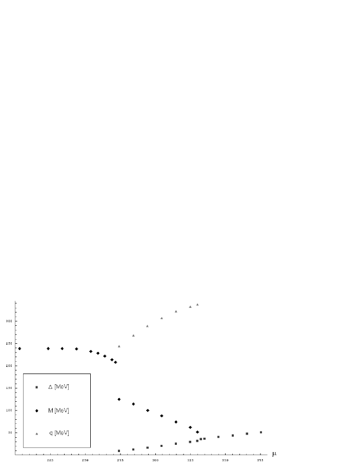
Figure 4: The phase diagram at one plot in 4D cut-off regularization schemes (in MeV units).

The size of the non-uniform phase depends on the relative strength of $G^{\prime}$ and $G$ coupling constants. The larger $G^{\prime}$ constant the shorter range of the non-uniform phase. This conclusion is also independent of the regularization scheme.

Finally, we find that in the Pauli - Villars scheme, in contrast to the other schemes, there is no coexistence region of the non-uniform and 2SC phases. Thus such a coexistence remains an open question. Let us stress at the end that our analysis does not prove that the non-uniform chiral phase exists. However, it shows that the main features of the phase diagram which includes non-uniform phase are robust against the choice of the regularization schemes.

VI Appendix A

Two parameters of the NJL model ($G,\Lambda$) are fixed by two physical quantities: the pion decay constant $f_{\pi}=93$ MeV, and the quark condensate density $\left\langle\bar{u}u\right\rangle=\left\langle\bar{d}d\right\rangle=$-(250 MeV)³. These quantities are functions of $M_{0}$ and $\Lambda$, and can be calculated in the framework of the NJL model, as was done in klev . Alternatively one can use the decay constant $g_{\rho}$ for the $\rho\rightarrow 2\pi$ process instead of the quark condensate value, proposed in blasz . Now using the self-consistency condition, $M_{0}$ = $-4G\left\langle\bar{u}u\right\rangle$, that links $G$ and $\Lambda$ with $M_{0}$, we get values of $G$ and $\Lambda$.

In different regularization schemes, one has

• 3D cut-off

  $$\left\langle\bar{u}u\right\rangle=-6M_{0}\int^{\Lambda}\frac{d^{3}k}{(2\pi)^{3}}{\frac{1}{E_{0}}},\;\;\;f^{2}_{\pi}=3M_{0}^{2}\int^{\Lambda}\frac{d^{3}k}{(2\pi)^{3}}{\frac{1}{E_{0}^{3}}}.$$

• 4D cut-off

  $$\left\langle\bar{u}u\right\rangle=-12M_{0}\int^{\Lambda}\frac{d^{4}k_{E}}{(2\pi)^{4}}{\frac{1}{E_{0}^{2}+k_{0}^{2}}},\;\;\;f^{2}_{\pi}=12M_{0}^{2}\int^{\Lambda}\frac{d^{4}k_{E}}{(2\pi)^{4}}{\frac{1}{(E_{0}^{2}+k_{0}^{2})^{2}}}.$$

• Schwinger

  $$\left\langle\bar{u}u\right\rangle=-\frac{3}{4\pi^{2}}M_{0}\int^{\infty}_{1/\Lambda^{2}}\frac{d\tau}{\tau}{\exp[-\tau M_{0}^{2}]},\;\;\;f^{2}_{\pi}=\frac{3}{4\pi^{2}}M_{0}^{2}\int^{\infty}_{1/\Lambda^{2}}\frac{d\tau}{\tau}{exp[-\tau M_{0}^{2}]}.$$

• Pauli-Villars

  $$\left\langle\bar{u}u\right\rangle=\frac{3}{4\pi^{2}}M_{0}\left\{\sum^{3}_{\alpha=1}C_{\alpha}M_{\alpha}^{2}\ln\left[\frac{M^{2}}{M_{\alpha}^{2}}\right]\right\},\;\;\;f^{2}_{\pi}=\frac{3}{4\pi^{2}}M_{0}^{2}\left\{\sum^{3}_{\alpha=1}C_{\alpha}\ln\left[\frac{M^{2}}{M_{\alpha}^{2}}\right]\right\}$$

  with three conditions impose on regularization parameters

  $$1+\sum^{3}_{\alpha=1}C_{\alpha}=0,\;\;\;M^{2}+\sum^{3}_{\alpha=1}C_{\alpha}M_{\alpha}^{2}=0,\;\;\;M^{4}+\sum^{3}_{\alpha=1}C_{\alpha}M_{\alpha}^{4}=0.$$ (12)

  Conditions (12) are solved by the formulae:

  $$C_{1}=-3,\ C_{2}=3,\ C_{3}=-1,\ M_{1}^{2}=M^{2}+\Lambda^{2},\ M_{2}^{2}=M^{2}+2\Lambda^{2},\ M_{3}^{2}=M^{2}+3\Lambda^{2}$$ (13)

The values of $G,\Lambda$ for each regularization scheme are given in Table I.

Acknowledgement This research was supported by the MEiN grant no. 1P03B 045 29 (2005-2008).

References

- (1) M. Alford, K. Rajagopal and F. Wilczek, Phys. Lett. B422 (1998) 247; R. Rapp, T. Schafer and E. V. Shuryak, Phys. Rev. Lett. 81 (1998) 53; D.T. Son, Phys. Rev. D59 (1999) 094019.
- (2) A. I. Larkin and Yu. N. Ovchinnikov Zh. Eksp. Teor. Fiz. 47 (1964) 1136; P. Fulde and R. A. Ferrell, Phys. Rev. bf 135 (1964) A550, M. Alford, J. A. Bowers and K. Rajagopal, Phys. Rev. D63 (2001) 074016, J. A. Bowers, J. Kundu, K. Rajagopal and E. Shuster, Phys. Rev. D64 014024, J. A. Bowers and K. Rjagopal, Phys. Rev. D66 065002.
- (3) D. V. Deryagin, D. Yu. Grigoriev and V. A. Rubakov, Int. J. Mod. Phys. A7 (1992) 659, B.-Y. Park, M. Rho, A. Wirzba and I. Zahed, Phys. Rev. D62 (2000) 034015, R. Rapp, E. Shuryak and I. Zahed, Phys. Rev. D63 (2001) 034008.
- (4) F. Dautry, E. M. Nyman, Nucl. Phys. A319 (1979) 323, T. Tatsumi, Prog. Teor. Phys. 63 (1980) 1252. M. Kutschera, W. Broniowski and A. Kotlorz, Nucl. Phys. A516 (1990) 566; Phys. Lett. B237 (1990) 159, M. Sadzikowski and W. Broniowski, Phys. Lett. B488 (2000) 63
- (5) M. Sadzikowski, Phys. Lett. B642 (2006) 238.
- (6) W. Broniowski and M. Kutschera, Phys. Lett. B242 (1990) 133.
- (7) M. Sadzikowski, Phys. Lett. B553 (2003) 45.
- (8) S. P. Klevansky, Rev. Mod. Phys. 64 (1992) 649.
- (9) E. Nakano and T. Tatsumi, Phys. Rev D71 (2005) 114006.
- (10) M. Buballa and M. Oertel, Nucl. Phys. A 703, (2002) 770.
- (11) D. Blaschke, M. K. Volkov, and V. L. Yudichev, Eur. Phys. J. A17 (2003) 103.