On the growth and stability of Trojan planets

Abstract

Aims. We investigate the stability of those low-mass Trojan planets that form in a protoplanetary disc and subsequently accrete gas to become gas giants.

Methods. We calculate their evolution before, during, and after gas disc dispersal. A two-dimensional hydrodynamics code combined with an $N$-body solver is used to evolve the system of disc and planets. Gas disc dispersal is simulated in a simple manner by assuming global exponential decay of the disc mass, leading to the stalling of migration after semi-major axes have approximately halved from their initial values. We consider Trojan pairs with different initial masses and gas accretion rates and gas disc models with different masses and viscosities. An $N$-body code, adapted to model disc forces, is used to examine large-scale migration and the formation of very short period Trojan planets.

Results. For each combination of planetary pair and disc model that we consider in our hydrodynamic simulations, each Trojan system remains stable before, during, and after disc dispersal. The long-term stability of these systems in the absence of gas is tested using $N$-body simulations, and all systems remain stable for those evolution times equal to $10^{9}$ years. Eccentricities remain low ($e<0.02$) in all cases. Increases in the amplitude of libration about the $L_{4}$/$L_{5}$ Lagrange points accompany the inward migration, and during very large-scale migration Trojan systems may be disrupted prior to the onset of disc dispersal.

Conclusions. The stability of Trojan pairs during rapid type I migration, during the transition to type II migration with the accompanying gap formation in the gas disc, and during gas loss when the disc disperses, indicates that isolated Trojan planet systems are very stable. If a common mechanism exists for their formation, we suggest they may be readily observed in nature.

1 Introduction

As we become aware of an ever-increasing number of exoplanetary systems containing multiple planets, we find that the vast majority thus discovered all differ greatly in some manner from our own Solar System (Fischer et al. 2008; Cochran et al. 2007; Udry et al. 2007). Some potential planetary system architectures have been hypothesized but not yet observed; however, among these are the Trojan planets: planetary pairs orbiting a star with very similar semi-major axes but with a leading/trailing separation in azimuth of $\simeq 60^{\circ}$. Nonetheless, such a discovery would not be completely without precedent. In our own solar system Jupiter and Neptune both possess sizeable populations of Trojan asteroids at their $L_{4}$ & $L_{5}$ points, while some satellites of the giant planets lie in co-orbital horseshoe (Janus & Epimetheus) and tadpole (Dione, Helene and Polydeuces) orbits.

One condition we may state with certainty is that Trojan planet formation requires the presence of multiple planets within a system. Current observations find that $\sim 10$% of observed planetary systems host multiple planets, a figure that is expected to increase as detections of lower-mass bodies increase in number with the recent and future launches of newer, more sensitive space missions (e.g. KEPLER, CoRoT).

Recent models of planetary formation have suggested different mechanisms by which Trojan planets may form. In-situ formation of a co-orbital companion, possibly through an enhanced local density of solids near the triangular Lagrange points of a massive planet has been suggested by Laughlin & Chambers (2002) and examined more recently by Beaugé et al. (2007). Other authors describe the capture of existing bodies into the $L_{4}/L_{5}$ points through a variety of mechanisms: the collision of two objects near a triangular Lagrange point or capture into a Trojan orbit due to rapid mass accretion by the primary planet (Chiang & Lithwick 2005); rapid convergent migration between a single gaseous and multiple rocky planets, directly into a co-orbital resonance (Thommes 2005); or the scattering of existing objects into the $L_{4}/L_{5}$ points either through large scale, global planetary system instability, during which the Trojan asteroids in our Solar System may have been captured (Morbidelli et al. 2005), or local gravitational scattering during the violent relaxation of a closely packed planetary system (Cresswell & Nelson 2006, 2008). If capture in a co-orbital resonance occurs during or prior to planetary migration, the libration amplitude of the oscillations may be decreased; numerical simulations have shown this to occur for both gaseous discs (Cresswell & Nelson 2008) and planetesimal ones (Ford & Holman 2007). This damping causes initial horseshoe orbits to become tadpole orbits around one or other of the $L_{4}$/$L_{5}$ Lagrange points. Three-dimensional hydrodynamic simulations indicate that co-orbitals formed from planetary scattering typically lie in or near the disc midplane, and in any case the presence of a gaseous disc rapidly damps the inclination of a companion body into the same plane as its primary (Cresswell & Nelson 2008).

Table 1: Table summarising the differences between each model run.

Model	$m_{\rm{t,i}}$	$m_{\rm{l,i}}$	$f_{\rm{l}}$	$\alpha$	$M_{\rm{disc}}$	$m_{\rm{t,f}}$	$m_{\rm{l,f}}$	$q_{\rm{p}}$
	($M_{\oplus}$)	($M_{\oplus}$)				($M_{\oplus}$)	($M_{\oplus}$)
1	15	15	5/3	$5\times 10^{-3}$	1	145	125${}^{\mbox{\tiny{\it 1}}}$	$0.862^{\mbox{\tiny{\it 1}}}$
2	15	15	5/3	$5\times 10^{-3}$	0.5	141	172	0.817
3	15	15	5/3	$10^{-3}$	1	$\sim 125$	$\sim 100^{\mbox{\tiny{\it 2}}}$	$\sim 0.75^{\mbox{\tiny{\it 2}}}$
4	15	1	0	$5\times 10^{-3}$	1	185	1	$5.40\times 10^{-3}$
5	15	10	5/3	$5\times 10^{-3}$	1	182	69	0.378
6	10	15	5/3	$5\times 10^{-3}$	1	62	191	0.324
7	20	10	5/6	$5\times 10^{-3}$	1	190	45	0.235

Models that produce co-orbitals because of dissipation provided by a disc may also experience significant inward migration, which would increase the probability of the planets’ detection. Many studies investigating the possibility of detecting Trojan planets focus on transit observations (Rowe et al. 2006; Ford & Holman 2007; Gaudi & Winn 2007) or a combination of transit and radial velocity methods (Ford & Gaudi 2006), since additional physical information may be obtained in the event of discovering a body with Earth-like properties. Observational constraints on Trojan formation will provide clues to the formation history of a planetary system, for example indicating that a period of violent relaxation has occurred in a highly dissipative environment (Cresswell & Nelson 2006, 2008), or for short period systems differentiating between circularisation near the star of an initially highly eccentric orbit versus migration through a gaseous disc.

In this paper we consider Trojan systems that have been formed within a gaseous protoplanetary disc. Implicit in our assumption is that the formation mechanism is the same as that proposed by Cresswell & Nelson (2006, 2008), since the Trojan systems we consider are similar to those found as intermediary or end-states of the simulations in Cresswell & Nelson (2008). We follow their evolution as they migrate and accrete gas from the disc, through the epoch of gas disc dispersal, and finally in the disc-free environment to determine the stability of such pairs throughout a global history of the system.

This paper is organised as follows. In Sect. 2 we describe the models used, and in Sect. 3 we present our results. In Sect. 4 we conclude with a short discussion of the implications of this work for the detection of Trojan planets.

2 Numerical Methods

We use both hydrodynamic and modified $N$-body simulations in this paper. We first discuss the hydrodynamic scheme in Sect. 2.1, followed by the $N$-body method in Sect. 2.2.

2.1 Hydrodynamic method

Due to the comparatively short inclination damping time, we have found that in the presence of a protoplanetary disc most Trojan systems are quickly reduced to co-planarity (to within $<0.1^{\circ}$) and remain in that state in the absence of any further influences (Cresswell & Nelson 2008). In order to maximise the simulated time of our models on available hardware we therefore elected to utilise two-dimensional simulations of the disc-planets system.

We use the NIRVANA hydrodynamic code in two dimensions using $(r,\theta)$ co-ordinates (see Cresswell & Nelson (2006) for details). The computational domain is given by $[2,12.5]$ AU in radius and $[0,2\pi]$ radians in azimuth. The number of uniformly spaced grid cells used in the radial and azimuthal directions is $N_{r}=300$ and $N_{\theta}=900$, respectively. The disc is assumed to be locally isothermal with a constant aspect ratio $h=H/r=0.05$, and the surface density profile is given by $\Sigma(r)=\Sigma_{0}r^{-1/2}$. For most models $\Sigma_{0}$ is normalised such that the disc contains 0.04 $M_{\odot}$ of gas interior to 40 AU. We adopt a standard $\alpha$-model for the disc viscosity, such that the kinematic viscosity $\nu=\alpha c_{s}H$ where $c_{s}$ is the local isothermal sound speed (Shakura & Sunyaev 1973). At the inner radial boundary we use a viscous outflow condition to define the radial velocity (Pierens & Nelson 2008), such that $v_{r}=\beta v_{\rm{visc}}$, where $v_{\rm{visc}}(r)=-3\nu/2r$ is the inward drift velocity of a steady-state accretion disc. $\beta$ is a free parameter for which we choose $\beta=5$ in accordance with Pierens & Nelson (2008) and Crida et al. (2007); however other nearby values of $\beta$ were tested and found to produce no significant differences in the resultant planetary systems formed. The outer boundary is reflective with a wave-damping function adopted between $r=10.5$ and $12.5$ AU to minimize wave reflections (Cresswell & Nelson 2006).

We perform runs using a variety of initial planet masses and accretion rates (see table 1; from left to right, columns represent: model number, initial mass of trailing planet, initial mass of leading planet, accretion factor of leading planet, viscous $\alpha$-parameter, disc mass (normalised against model 1), final mass of trailing planet, final mass of leading planet, and final mass ratio of the two planets). The planets are initially in tadpole orbits in all models; initial positions and velocities are taken from a simulation in Cresswell & Nelson (2008), where a co-orbital pair has recently damped to stable, co-planar tadpole librations. Although in each run the planets will be librating around slightly different points with different amplitudes, in each case the planets’ orbits make the necessary adjustments within a few orbital periods, aided by the damping action of the surrounding disc. The planets’ orbits are evolved using a fifth-order Runge-Kutta method, and by calculating the torque from the disc on each planet; the torque from material located within one Hill radius of each planet is neglected from this torque calculation, using a Heaviside step function. A gravitational softening parameter $\epsilon=0.5H$ is used when calculating the planet potentials. The time step is calculated by determining separate N-body and hydrodynamical timesteps, and utilising the smaller value; further details are provided in Cresswell & Nelson (2006).

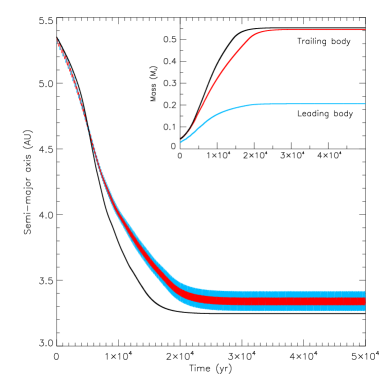
Figure 1: (Main) The semi-major axes of the leading (blue line) and trailing (red line) planets in model 5; note the oscillations in $\Delta a$ are larger for the leading body, so that the red line appears superposed above the wider blue line. Stable, near-circular tadpole orbits are retained at all times. The evolution of the same 15 M_⊕ planet in isolation is shown for comparison (black line). (Inset) The planets’ masses, in Jupiter masses, over the same time frame.

Accretion onto the planets is handled in a similar way to D’Angelo et al. (2003), with the density within 0.1 Hill radius of the planet reduced by a factor $1-f\Delta t$ during each time step. As with Paardekooper & Mellema (2008), we choose $f=5/3$ in most models, but other values are used for the accretion rate onto the leading planet (labelled $f_{\rm{l}}$ in table 1) in some cases.

Each simulation progresses until one planet reaches a prescribed mass, whereupon at each iteration the mass of the disc is reduced everywhere according to an exponential decay law with an $e$-folding time of approximately 2550 years. This prescribed value is usually 0.5 Jupiter masses ($M_{\rm{J}}$), although in some cases (models 1 & 3) where both planets possess the same initial mass this value cannot be achieved prior to the planets migrating all the way to the inner boundary. This occurs because systems with the same initial masses usually show a reduced rate of accretion onto both planets as they compete for gas. In these cases a lower value is taken for the planet mass at which gas dispersal is initiated. See table 1 for further details of each run. After approximately a further $1.2\times 10^{4}$ years of disc mass reduction, disc forces are disabled completely (i.e. the system is purely $N$-body) to determine stability without the effect of the disc. Although disc dispersal time scales are believed to be 2 – 3 orders of magnitude longer than those used here, the rapid decay we employ makes the transition from embedded to free planets computationally tractable. Test simulations of resonant planets using HENC-3D (an $N$-body code adapted to emulate the effects of hydrodynamic disc forces, see Sect. 2.2) have shown that as long as the decay time scale is not near-instantaneous, the rate at which disc mass is removed is not responsible for determining whether the resulting system remains stable in the absence of a surrounding disc. The time scale we use is longer than any of the natural dynamical time scales involved in the problem, including the secular evolution time for the planet orbits, suggesting that our gas dispersal algorithm should be reasonably successful in capturing the process of slow disc dispersal.

2.2 $N$-body method

At the present time it is not possible to run hydrodynamic simulations for sufficient time to simulate very large scale migration of Trojan planet pairs. The simulations performed using NIRVANA included a routine for modelling disc dispersal that normally switches on when the planet semi-major axes have approximately halved from their initial values. To simulate the formation of short-period Trojans we use an $N$-body code adapted to emulate hydrodynamic forces, HENC-3D (see Cresswell & Nelson (2008) for details). The migration and eccentricity and inclination damping rates of HENC-3D are founded on the analytic prescriptions of Tanaka & Ward (2004) and Papaloizou & Larwood (2000), and are calibrated against NIRVANA to provide good approximations to the migration and eccentricity (and inclination) damping rates; it utilises the same fifth-order Runge-Kutta integrator as NIRVANA. Since this $N$-body code uses semi-analytic terms to model the disc forces rather than modelling the disc itself and calculating the resultant force, mass accretion is simulated using a hyperbolic tangent function, tailored to each model, such that planets reach the same final mass at the same time as their counterparts in the hydrodynamic models. Independently of their growth, after an appropriate time the disc forces are reduced to simulate excavation of a gap and the reality that the type I forces modelled by HENC-3D would be too large for a body that has accreted significant amounts of gas. Both of these additions were tested against all the models used by HENC-3D to ensure agreement with NIRVANA before further simulations beyond NIRVANA’s capacity for inward migration were conducted. Disc dispersal was modelled to occur on the same time scale to that described above for the NIRVANA simulations, and was mimicked by simply reducing the disc forces using an exponential decay law.

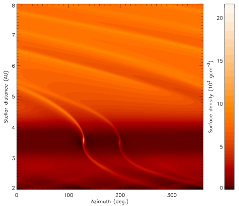
Figure 2: Surface density of the inner region of the disc in model 5 at $t\approx 16,700$ yrs. The planets’ masses at this time are 156 $M_{\oplus}$ (left) & 65 $M_{\oplus}$ (right).

3 Results

3.1 Orbital evolution

We begin by describing the orbital evolution of the Trojan systems. Fig. 1 shows the evolution of the semi-major axes for the two planets in model 5, whose initial masses were 15 and 10 M_⊕, and final masses after disc dispersal were 182 and 69 M_⊕. The two planets migrate inward at close to the standard type I migration rate as they accrete gas, and remain stable throughout their evolution. The initial phase of inward type I migration occurs because of our adoption of a locally isothermal equation of state. Paardekooper & Mellema (2008) have shown that migration in a radiatively inefficient disc may be stalled or reversed, but once gap formation ensues the corotation torques responsible for this should decrease, leading to long-term inward migration. Also plotted in Fig. 1 is the semi-major axis evolution of an isolated 15 M_⊕ planet undergoing the same accretion process. Comparison between the migration rates shows that the Trojans begin to migrate slightly faster early on in their evolution as their masses grow and type I migration rates increase, but as gap formation starts to occur, and disc dispersal is switched on, their migration begins to slow before finally halting after the gas disc has been completely removed. The inset to Fig. 1 shows that the growth of one planet is accompanied by the inhibition of the accretion rate of its companion; however the larger body does not accrete at the same rate as the equivalent isolated planet, with its Trojan partner removing some of the material in the horseshoe region. Divergence of the masses of the Trojan planets during migration means that their individual migration rates should also diverge, but the 1:1 resonance is maintained during migration, causing the planets to migrate inward in lock step. The long term evolution in the absence of gas consists of the planets orbiting stably at their mutual $L_{4}$/$L_{5}$ Lagrange points, with small amplitude librations in semi-major axes caused by the libration associated with the tadpole orbits. Although initially damped to small librations by the disc, as the planets migrate inwards the amplitudes of these librations increase slightly, but always remaining firmly within the tadpole regime over the radial distances covered here (but see Sect. 3.4 for a discussion about the evolution during large-scale migration). The orbital eccentricities remain small during migration, increasing slightly upon gas disc removal but always remaining below $e=0.02$.

Figure 2 shows the surface density of the inner disc in model 5 after approximately $1.67\times 10^{4}$ years, shortly before disc dispersion is applied. By this time the two bodies have cleared a significant gap in the disc, though the larger body dominated the local dynamics. Some wave reflection is visible at the inner boundary; the planets in different models ceased migration (due to disc dispersal) at varying distances from the inner boundary, some close to the depleted inner edge of the disc and within range of the reflected waves, and some not, but no discernible effects in the evolution of any Trojan pair was observed as a result. Indeed, with the exception of the final orbiting radius, the orbital evolution and surface density profile of each model was very similar.

We note here that our adoption of a ‘viscous outflow’ boundary condition prevents rapid loss of the inner disc as is observed when open boundary conditions are used. Our adoption of an outflow velocity maximum that is five times larger than the nominal viscous rate, however, can still cause the inner disc to deplete a little too rapidly. Potentially this could affect the outcome of our results, and so we have run tests in which the outflow velocity maximum was varied with both larger and smaller values used. We find that our results are insensitive to the adopted values.

With only minor variations in description, this summary applies equally to all of models 1 – 7, indicating that Trojan planets are generally stable and insensitive to their relative masses and local disc conditions, at least within the parameter ranges considered in these hydrodynamic simulations. In agreement with Cresswell & Nelson (2006, 2008) Trojans also remain stable throughout significant migration, including during the rapid migration which occurs as the planets grow but prior to gap formation. The onset of gap formation during the evolution of model 5 is shown in Fig. 2, which displays a snapshot of the disc surface density profile. The position of the planets is clearly visible within the gap caused by the combined effects of gas accretion and the tidal torques induced by the trailing planet, whose mass at this point in time has almost reached 0.5 M_J.

3.2 Planetary mass growth

3.2.1 Equal initial planet masses

In models 1 – 3 the planet masses at the beginning of the simulations were all 15 M_⊕, with leading and trailing planets having the same mass. In model 1 the migration rate of the planets was such that they both began to approach the inner boundary of the computational domain prior to either of them reaching 0.5 M_J, the mass at which gas disc dispersal is switched on. Therefore, in this model, gas disc dispersal was initiated when the most massive planet had reached $m_{t}=0.41$ M_J. The evolution of the planet masses is shown in Fig. 3, and the final masses are listed in table. 1. For the case of model 1 it can be seen that the planet masses remain similar during the evolution, but there is a slight divergence with the trailing planet being the larger one.

Model 2 used a very similar set up to model 1, except the disc surface density everywhere was halved. This caused the migration to slow, and allowed the planetary growth to proceed until one of the planets reached 0.5 M_J, after which gas disc dispersal was initiated. Interestingly, we find that the planet masses in this case also remain similar during the evolution, but in this instance the leading planet becomes the larger one, in contrast to the situation in model 1. This indicates that in general, when Trojan planets of equal mass begin to accrete gas at the same time their masses will remain similar, but some level of divergence will occur due to stochastic changes in the accretion rates as the system evolves. Our simulation sample is too small to indicate any underlying bias between the leading or trailing planets becoming the more massive, but does show that either the leading or trailing planet may grow faster. Once the planetary mass ratio diverges from unity, then the simulations indicate that the divergence tends to accelerate, for reasons discussed in the following subsection.

Model 3 used very similar parameters to model 1, except the disc viscosity was reduced from $\alpha=5\times 10^{-3}$ to $10^{-3}$. During the process of gap opening this allows the gap to deepen more quickly, since material is less able to viscously diffuse into the gap. With the added effect that the planets are competing for the same material to fuel their growth, the result is that the planets grow significantly slower and end up with smaller masses, as shown in table. 1. The slow growth of these planets caused them to migrate close to the inner boundary before reaching 0.5 M_J, and the simulation was simply halted at this point.

Figure 3: Planetary masses for a selection of models; all planets shown had reached their final mass before $4\times 10^{4}$ yrs.

3.2.2 Unequal initial planet masses

Models 4 – 7 all started with unequal initial planet masses. In model 4, the trailing planet had a mass of 15 M_⊕ and was able to accrete at the normal rate, but the leading planet had a mass of 1 M_⊕ and was unable to accrete since this mass is below the critical core mass for gas accretion (Pollack et al. 1996). This model simply serves to show that a Trojan system which forms with an Earth-like planet component can evolve stably to the stage where the primary component is a gas giant.

Models 6 and 7 have initial planet masses of 10 and 15 M_⊕, and differ only in which of these planets is leading or trailing. Prior to gap opening, the larger Hill radius of the more massive planet causes this larger planet to have a higher accretion rate, causing the initial mass difference to grow. As gap formation begins to occur, viscous gas flow into the gap from the main body of the disc allows the more massive planet with the largest Hill radius to dominate the accretion process, since it is able to intercept this gas before the smaller planet can. The dominating body proceeds to accrete disc mass while depriving its less massive companion of material, and the mass ratio between the two planets moves successively further from unity; this is demonstrated in the inset to Fig. 1 which shows the evolution of planet masses for model 5, and in Fig. 3 which shows the evolution of both models. With the formation of a deep gap in the disc, the accretion rate of the smaller planet falls to near-zero while that of the larger body follows linear growth (until disc mass reduction begins). In our simulations, the mass of the smaller body is typically capped at 50 – 70 $M_{\oplus}$ when the initial planet masses are unequal, while the accretion rate of the larger body is largely unaffected by the presence of a companion. We performed additional test calculations with initial conditions similar to models 5 and 6, but with gas disc dispersal switched off. In those models we also found that the accretion of gas by the less massive planet was also diminished when gap formation by the heavier planet ensued, resulting in final masses of between 50 – 70 M_⊕ for the lighter planet. This shows that these final masses are not a product of the gas disc dispersal, but because the lighter planet becomes starved of gas when gap formation occurs.

In model 7 the trailing planet is twice as massive initially as the leading planet (20 versus 10 M_⊕). In addition the lower mass planet had a slower gas accretion rate, as might be expected from detailed models of gas accretion onto solid planetary cores (Pollack et al. 1996). In light of the naturally diverging accretion rates among all the Trojan pairs we studied, the differing accretion prescriptions merely exacerbates the effect. Consequently the results of this simulation are rather unsurprising: the initially unequal planet mass ratio becomes more unequal during the evolution, and the system remains stable for the duration of the simulation.

It is worth commenting that our models of accreting Trojans indicate that two accreting ice and rocky planetary cores are able to clear a gap in the disc quicker than an isolated planet. For example, after $5\times 10^{3}$ years the azimuthally-averaged surface density at the radial location of the planet ($\Sigma_{\rm{p}}$) is observed to be 15% lower in model 5 than in the case of an isolated $15M_{\oplus}$ planet, and 27% lower in model 1. The gap in both cases is also excavated quicker, having up to a 50 – 60% lower value of $\Sigma_{\rm{p}}$ after 0.5 – $3\times 10^{3}$ years. One interesting by-product of this is that the Trojan pairs will spend less time undergoing type I migration than an isolated, accreting planetary core, helping prolong their life time in the disc.

3.3 Long term stability

We have run all models 1 – 7 for $10^{9}$ years in the absence of gas, and find all systems to be stable, with no long term increases in eccentricity or libration amplitudes in semi-major axes. These results indicate that Trojan planet systems consisting of at least one gas giant planet and possibly two, at the distances from the star considered previously, are extremely stable during and after their formation.

3.4 Formation of short-period Trojans

The Trojans in our NIRVANA simulations are limited to migrating to within a few AU of the star, having formed with semi-major axes $\simeq 5.3$ AU. To observe the stability of Trojan planets as they migrate to much smaller radii, we use the HENC-3D $N$-body code described in Sect. 2.2, which provides a reasonable approximation of the hydrodynamic forces at work.

The models are run as follows: for each of the models 1, 4 & 5 described in table 1, the relevant Trojan pair is allowed to migrate all the way towards the star without disc dispersal. Each run is then repeated with disc dispersal simulated once the the semi-major axis of the more massive planet reaches 0.5, 1.0 or 1.5 AU. These runs are repeated a further three times for all cases using a small random perturbation of the initial conditions, including a vertical displacement not possible in the 2D NIRVANA runs, to generate a set of four distinct tadpole pairs for each initial mass ratio and stopping distance.

As noted in the NIRVANA models (Sect. 3.1, see Fig.1 in particular), after a brief initial period of decrease, the amplitude of the tadpole librations slowly increases as the planets migrate inward. Those planets stopped by simulated disc dispersal at distances of $\approx 0.5$ AU from the star always survived in tadpole orbits, with minimum/maximum ($\theta_{\rm{min}}$/$\theta_{\rm{max}}$) separations between the two planets of up to $\theta_{\rm{min}}\raisebox{-3.44444pt}{$\buildrel\textstyle>\over{\sim}$}25^{\circ}$ and $\theta_{\rm{max}}\raisebox{-3.44444pt}{$\buildrel\textstyle<\over{\sim}$}130^{\circ}$. However, the libration amplitude of those planets allowed to migrate further continues to increase until the system becomes unstable. Dissociation of the co-orbital pair is usually first signified by a shift from tadpole to horseshoe orbits, which typically last for less than $3\times 10^{4}$ yrs (although horseshoe orbits lasting over $10^{5}$ were also observed). This is finally followed by either collision (76% of cases) or scattering onto distinct orbits. In one instance differential migration caused the two bodies to form a 5:3 mean motion resonance (MMR) after scattering.

This amplitude increase and eventual destruction of the co-orbital structure was observed regardless of the initial mass ratio and, in further tests, the migration and eccentricity damping rates of the disc. After starting their migration from 5.3 AU in our simulations, in all cases the instability took effect between 0.5 – 0.1 AU.

We also performed numerical experiments which involved: (i).  placing planets on initial tadpole orbits with smaller libration amplitudes; (ii).  retaining the original libration amplitudes but placing planets closer to the star initially. Both of these changes allow planets to remain on tadpole orbits while migrating very close to the star (i.e. Trojans with semi-major axes $\leq 0.1$ AU), raising the possibility that ‘hot Trojans’ containing a gas giant planet component may form and survive. The potential observability of such systems is therefore highly dependent on the initial orbits of the planets when the Trojan systems are established, and the ability of the disc to damp large initial librations directly after the Trojan systems have formed.

We note that, despite the abundance of Trojans ($\sim 30$%) in the simulations of Cresswell & Nelson (2008), the disruption of these systems during large-scale migration was not always detected there. After re-examining that data we note that this stability was found to occur only in Trojan systems which were also in a mean motion resonance with another body. Apparently this additional body is able to provide a stabilising effect, allowing a Trojan system to migrate closer to the central star. We note however that an additional body did not always provide a stabilising influence, and similar scattering behaviour was observed in some of the runs presented in Cresswell & Nelson (2008).

4 Discussion and conclusions

We have investigated the evolution of so-called tadpole or Trojan planets, whose masses are initially in the Neptune-mass (or Earth-mass) range, in the presence of a gas disc from which they are able to accrete to become gas giant planets. For such an isolated pair, previously damped onto coplanar, near-circular orbits by the disc after the co-orbital configuration was formed (as found by Cresswell & Nelson (2008)), we find that each pair remains stable during rapid type I migration and gas accretion from the disc. This period of stability also extends through the epoch of gap formation in the disc, and the period of gas disc dispersal, resulting eventually in Trojan systems which are stable for $10^{9}$ years.

For Trojan systems of planets with masses which were initially equal, we found that gas accretion resulted in final gas giant planets with similar but not equal masses. For systems with unequal initial masses, we find that the initially more massive body dominates the accretion and approaches the Jovian mass as if in isolation. The lower mass planet is effectively starved of gas when gap formation ensues, causing its final mass to not exceed 70 M_⊕, at least for the parameters we have considered. This suggests that Trojan planetary systems in nature consisting of one component which is a gas giant are likely to have a second component which is considerably smaller in mass.

Our results indicate that if a mechanism exists to form significant numbers of Trojan planets, such as the violent relaxation of a planetary system in the presence of a substantial gas disc (Cresswell & Nelson 2006, 2008; Morbidelli et al. 2008), then Trojans should be observed in nature as they are expected to be very stable, provided they have not undergone very large-scale migration. The simulations indicate that large disparities in mass are expected between the Trojan pairs, but detection of co-orbital systems with planetary masses in the Jupiter- and Saturn-mass ranges, or similarly-scaled Trojan pairs, will indicate a prolonged period of simultaneous co-orbital growth.

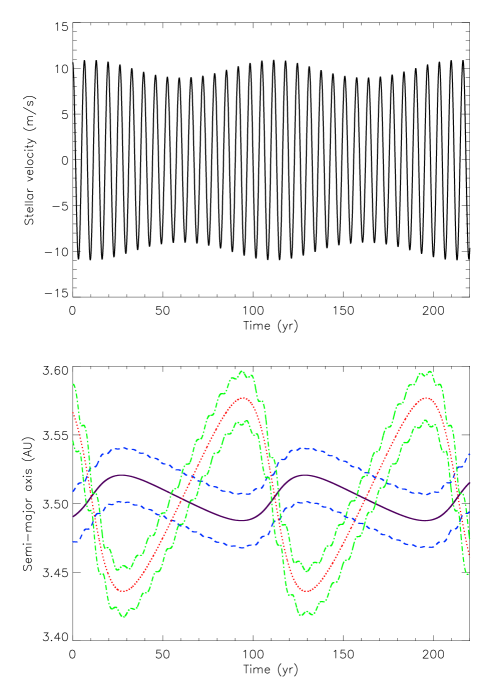
Figure 4: (Top) The radial velocity curve of a $1M_{\odot}$ star bearing a Trojan planetary pair, taken from the final state of model 7. (Bottom) The semi-major axes of the orbiting planets, with masses $190M_{\oplus}$ (continuous indigo line) and $45M_{\oplus}$ (dotted red line), over the same time. The instantaneous pericentres and apocentres of each planet are also shown.

We also find that inward migration produces an increase in the libration amplitude of Trojan planets about their mutual Lagrange points, eventually leading to instability and collision or planet-planet scattering if large-scale migration has taken place. This may have unfortunate implications for the detection of short-period Trojan planets containing one component which is a gas giant, since Trojan systems formed at $\simeq 5$ AU and with initial librations extending $\raisebox{-3.44444pt}{$\buildrel\textstyle>\over{\sim}$}15^{\circ}$ in azimuth from the $L_{4}$/$L_{5}$ point are expected to become unstable after they have migrated to within a few tenths of an AU of the central star. We expect that if such Trojan planets are observed, they will have entered into a co-orbital relationship somewhat closer to the star than in the simulations considered here, or have been damped by the disc onto — or otherwise formed with — much smaller tadpole librations before the opening of a gap. The simulations of Cresswell & Nelson (2008) produced Trojans that cover both of these possibilities, with initially large librations damped by the disc to a few degrees within a few $\times 10^{4}$ years. The formation of a planet at the Lagrange point (e.g. Beaugé et al. (2007)) may also produce sufficiently small librations to survive significant migration. Trojan pairs in mean motion resonance with a third body may also be subject to sufficiently small librations to survive large-scale migration.

As a means to reduce the effects of type I migration, Thommes (2005) suggested that gap-opening planets may provide a moving barrier by capturing fast migrators into mean motion resonances following behind the giant planet; in some instances multiple terrestrial bodies were observed to share the same MMR. Co-orbital capture of a terrestrial body with an (eventual) gas giant itself, in some cases even before gap-opening has begun, may serve the same function and act as a natural (and stable, in a post-disc environment) extension of this ‘stacking’ behaviour to include the 1:1 resonance with the giant planet itself. However, this does not address the prior issue of achieving a gap-opening planetary mass.

A sample radial velocity (RV) curve produced by a star orbited by a Trojan pair is shown in the top panel of Fig. 4. The tadpole motions of Trojan planets produce a regular variation in their semi-major axes, which is clearly visible in the star’s RV profile, amounting in this instance to a regular modulation in the curve’s amplitude of around 20%. In the given model the associated ‘beat’ has a period of approximately 100 yrs; if the planets were oscillating around 1 AU, this period would be only 17 yrs, with the peak amplitude of stellar radial velocities being modulated between 17 and 20 ms^-1; at 0.1 AU, this becomes $\sim$180 days and variations in the peak stellar radial velocity occurring between 53 and 64 ms^-1. Unfortunately the amplitude of this variation depends on the history of the system, since tadpole planets with minimal libration will show a very small variation, whereas systems with larger amplitude libration will show larger modulation of the radial velocity, so it is not a straightforward matter to define the expected amplitude of variation as a simple function of system parameters. The general shape of the RV curve, however, is a tell-tale sign of a Trojan system, and arises simply because the centre of mass of the system around which the star orbits varies with time as the planets librate around the $L_{4}$/$L_{5}$ points. When the planets are at their furthest distance apart in azimuth the system’s centre of mass lies closest to the central star, and its radial velocity amplitude is minimised. Conversely the centre of mass is at a maximum distance from the star when the planets are at closest approach, causing the radial velocity to be at a maximum. Our simulations suggest that variations in the radial velocity amplitude on the order of 10 – 20 % are expected in Trojan systems over time scales of about 20 orbital periods. This should allow short period gas giants with hot-Neptune Trojan companions to be discovered from radial velocity surveys, and if they exist, hot Neptunes with Trojan super-Earth companions. As mutual inclinations are expected to be small due to gas disc inclination damping, it is also possible that current and forthcoming transit surveys such as CoRoT and KEPLER will discover Trojan planet systems.