Climate Sensitivity and the Response of Temperature to CO₂

Abstract

A review of some of the evidence for the IPCC’s conclusion that doubling CO₂ levels will warm Earth significantly, in contrast to the claims of a recent articlemonckton . Simply looking at raw temperature and CO₂ data over the past 150 years gives a transient response of roughly 2 K per doubling, in good agreement with IPCC conclusions based on far more extensive analysis. The 0.58 K of Ref. monckton, is very unlikely.

I Introduction

As Spencer Weart has recently notedweart , many scientifically trained people seek a “straightforward calculation” of anthropogenic global warming, but “the nature of the climate system inevitably betrays a lover of simple answers.” The consensus estimates of the climate science community, expressed by the Intergovernmental Panel on Climate Change (IPCC) after years of struggling with these complexities, is that doubling atmospheric CO₂will result in a steady-state temperature increase (“equilibrium climate sensitivity”) of 2 to 4.5 K, with a best estimate of 3 K, and very unlikely to be less than 1.5 KIPCCAR4WG1 .

In a recent article in Physics and Societymonckton , Christopher Monckton presents a number of arguments that lead him to conclude that the IPCC estimate is wrong, and the correct value for sensitivity should be close to 0.58 K, well within the “very unlikely” range stated by the IPCC. I have listed elsewhereSmithMoncktonErrors over 100 errors of fact or logic, misinterpretations, invalid reasoning, or misleading statements in Monckton’s article. In many cases these invalid claims are not original with Monckton, but have been addressed repeatedly in the past. For example he uses at least ten of the “hottest skeptic arguments” found at skepticalscience.com: “It’s the sun”, “It’s cooling”, surface temperatures or models are unreliable, and so forth. Original with Monckton are a handful of numerical errors or misinterpretations of others’ work; I would refer those interested in such details to the list I have collectedSmithMoncktonErrors ; those who spot other errors are invited to contact me with details to be added to the list.

The central originality of Monckton’s article, which I will address in the following, is his breakdown of climate sensitivity into three components, and his further reasoning about those components. Monckton’s breakdown is implicit in much of the discussion about forcings and feedbacks in the IPCC reportIPCCAR4WG1 and review papers such as the one by Bony et alBonyFeedback . However, it must be emphasized that this breakdown into forcing, base response, and feedback factors is artificial and strictly valid only in a perturbative sense. It is useful for understanding what is going on, but it is not how sensitivity is actually determined. The IPCC consensus on sensitivity comes from model calculations and attribution studies that look at the response of the full climate system to changes in greenhouse gases, without breaking that response into a linearized “base” response and separate feedbacks. That is, the numerical values for base response and feedbacks, and to a lesser degree for forcings, the central concerns of Monckton’s article, are an output from the numerical models, not an input. They are a guide to understanding what is going on, and little more. So while Monckton’s breakdown is useful in the sense of being more explicit than is typically done, it is not in any sense a replication of the manner in which sensitivity is determined by the IPCC, since he does not derive his numbers from climate models. In fact in his treatment of the 2007 IPCC numbers he manages to get both forcing and feedbacks off by 10 to 20%, while coming to roughly the right final valueSmithMoncktonErrors .

II Sensitivity Reconsidered, Reconsidered

But it is the “reconsidered” sections of Monckton’s article which merit the most attention. The entire “radiative forcing reconsidered” section argues not about forcing at all, but about the temperature changes expected from forcings. Monckton ends by claiming he can divide the 3.7 W/m² forcing from doubling CO₂ by a factor of 3 because a certain temperature response is low – but this has nothing to do with the forcing at all, which is completely determined by the underlying physics. If anything, this section is an argument about feedbacks – but it is not phrased in that way, and so at the least is highly confusing.

Monckton culls a figure from the latest IPCC report (Monckton’s figure 4, IPCC AR4 WG1 figure 9.1IPCCAR4WG1 ) which is discussed at length in section 9.2.2.1, “Spatial and Temporal Patterns of Response”, but then misinterprets it. The image is based on estimates of forcing changes from 1890 to 1999. The strongest pattern is in the greenhouse gas image, because that is where the largest forcing change has occured. But the surface and low-altitude warming (or cooling) patterns are essentially the same across all the forcings – as the IPCC discussion puts it: “Solar forcing results in a general warming of the atmosphere with a pattern of surface warming that is similar to that expected from greenhouse gas warming, but in contrast to the response to greenhouse warming, the simulated solar-forced warming extends throughout the atmosphere.” The spatial pattern of response between different forcings differs only in the contrast between lower atmosphere and upper atmosphere: for solar forcing the warming happens everywhere, while for greenhouse forcing the upper atmosphere (stratosphere) cools while the surface and lower atmosphere warm. This differential in temperature change is readily observed, as Monckton’s figure 6 shows: warming at the surface, and cooling in the stratosphere. This is observational proof that the sun cannot be behind recent warming.

The tropical mid-troposphere “hot spot” that Monckton highlights is not a “fingerprint” of greenhouse gases: it is well known to be a consequence of higher water vapor levels in a warmer world, whatever the cause of the warming. As warm air rises, it cools almost adiabatically – this is known as the “lapse rate”, and stability of the atmosphere ensures that temperatures fall no faster than this rate with altitude. When air holding water vapor rises and cools, some of the water condenses and releases heat, resulting in warmer air at a given altitude, and a lower lapse rate. The strongest effect should show up in the tropical mid-troposphereSanterTropics , hence a “hot spot”. The observations are still being disputed, as even Monckton admits by refering to the wind-based measurements of Allen et al. Whatever the measurements and theory sort themselves out to on this, note again that tropical mid-troposphere temperature trends are not a signature of greenhouse gases, and this whole argument has no bearing on CO₂ forcing. Monckton has not made any case for arbitrarily dividing the forcing by 3 as in his equation 17. That would require drastically changing the spectroscopic properties of atmospheric constituents, for which there is certainly no justification in the arguments presented.

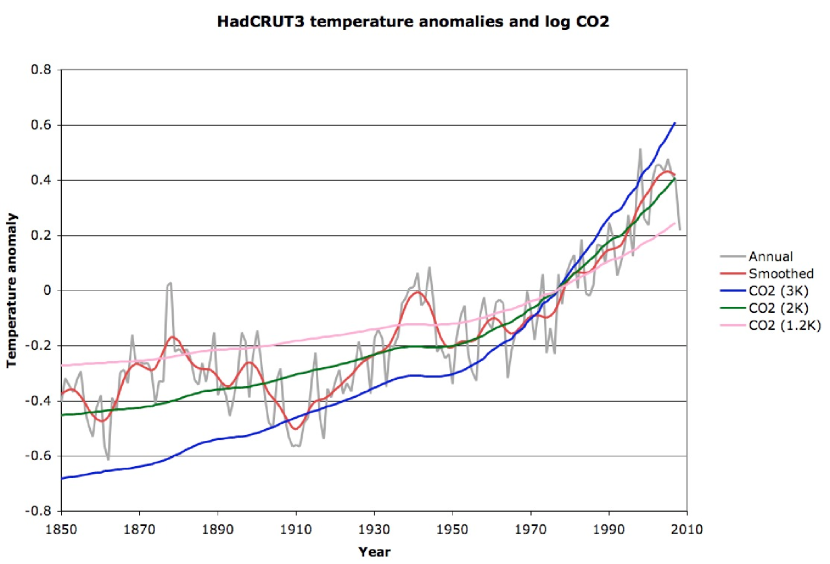
Figure 1: The gray curve is annual average temperature anomaly from the Hadley centerHadCrut3 , and in red is the corresponding 21-point smoothed curve. The other three lines plot the logarithm of CO₂ concentrations measured at Mauna LoaMaunaLoa and the 20-year smoothed Law Dome measurementsLawDome multiplied by appropriate sensitivity-to-doubling numbers and adjusted to a 0 average for the HadCRUT3 baseline period 1961 to 1990. Other than the sensitivity number there is no free parameter here; this is entirely derived from observations.

In his second “reconsidered” section, Monckton’s errors of logic and interpretation are spread thickest, on a matter for which there is again no real dispute. Similar to (in fact much more so than for) the forcing, the “base” response of the climate system is tightly constrained by the spectroscopic properties and temperature profile of the atmosphere, and is easily calculated in any model. The Soden and Held (2006) review paper refered to by Bony et alBonyFeedback provides two tables which show this base or “Planck” response as calculated from a variety of models. The range of what amounts to the inverse of Monckton’s $\kappa$ parameter is from 3.13 to 3.28 W/K m^2, with a mean of 3.22 and standard deviation of 0.04, or just over 1%. There is almost no uncertainty over the value of this number, despite the confusion Monckton fosters.

Finally, on the feedback factor f, and in particular the sum b of the feedback parameters, Monckton argues that the individual feedbacks must be too high because adding them plus their standard deviations leads to instability. He also quotes two papers that suggest that water vapor and cloud feedbacks are overstated by the climate models. The argument of the first “reconsidered” section on forcings, while completely irrelevant to forcings, if it had any validity would reinforce the suggestion of a reduced value for feedbacks. Nevertheless, Monckton here does the most mystifying thing in his entire article – he is “prudent and conservative” and retains the same (excessively high) value for the feedback sum b he has been using throughout the article.

But it is the feedbacks that are the most scientifically uncertain issues, by far the hardest things for modeling to get right, and the reason you cannot determine climate sensitivity from a one-page simple straightforward calculation. Getting the complex water vapor, cloud, lapse rate (convection and latent heat) and other responses to temperature changes sorted out is what makes climate modeling so tough. The feedbacks are the source of almost the entire uncertainty range in the IPCC’s estimate of climate sensitivity (which also relies on measurements of recent and ancient climate). Somehow Monckton treats the least certain quantity of the three in his breakdown as the most certain, while wildly reducing the values of the other two. His final estimate (equation 30) is not believable on these and other grounds, including his many other errorsSmithMoncktonErrors .

III Simpler Evidence

The simplest evidence I have seen that feedbacks are likely to be positive comes not from calculations but from measurements, dependent on the IPCC’s radiative forcing calculations (table 2.12IPCCAR4WG1 ) where the forcings from 1750 to 2005 due to all sources except CO₂ almost cancel out (the net total is about 10% of the CO₂ effect, with considerable uncertainty). That means an estimate of transient climate response to increased CO₂ can be found by plotting the historically measured atmospheric CO₂ values on the same chart as the historical temperature anomalies, over the past 150 years as is done in Figure 1.

The best fit to observed temperature is for a transient response of about 2K per doubling of CO₂. This compares well with the IPCC range of transient climate response of between 1 K and 3.5 K (see section 9.6.2.3 of IPCC AR4 WG1 IPCCAR4WG1 . The fact that the 20^th century rise in temperatures was of almost exactly the expected size is pretty strong evidence that the IPCC’s transient and equilibrium climate sensitivity numbers match reality. In particular, the equilibrium sensitivity is unlikely to be as low as the 1.2 K found with no feedbacks, and nowhere near the 0.58 K that Monckton claims.

IV Acknowledgments

I am grateful to several friends and colleagues for comments; this work has received no funding or support from any source.

References

- (1) Christopher Monckton: “Climate Sensitivity Reconsidered”, Physics and Society, 37, issue 3, p. 6 (2008)
- (2) Spencer Weart: “Simple Question, Simple Answer … Not”, RealClimate, 8 September 2008, http://www.realclimate.org/index.php/archives/2008/09/simple-question-simple-answer-no/ - see also Weart’s history website: “The Discovery of Global Warming”, http://www.aip.org/history/climate/
- (3) IPCC, 2007: Climate Change 2007: The Physical Science Basis. Contribution of Working Group I to the Fourth Assessment Report of the Intergovernmental Panel on Climate Change [Solomon, S., D. Qin, M. Manning, Z. Chen, M. Marquis, K.B. Averyt, M.Tignor and H.L. Miller (eds.)]. Cambridge University Press, Cambridge, United Kingdom and New York, NY, USA.
- (4) Arthur Smith, “A detailed list of the errors in Monckton’s July 2008 Physics and Society article”, http://altenergyaction.org/Monckton.html
- (5) S. R. Bony et al.: “How well do we understand and evaluate climate change feedback processes?”, Journal of Climate 19, p. 3445 (2006).
- (6) B. D. Santer et al., “Amplification of Surface Temperature Trends and Variability in the Tropical Atmosphere” Science 309, 1551 (2005).
- (7) Hadley Center temperature series: http://hadobs.metoffice.com/hadcrut3/diagnostics/global/nh+sh/annual
- (8) Mauna Loa CO2 series: ftp://ftp.cmdl.noaa.gov/ccg/co2/trends/co2_annmean_mlo.txt
- (9) Law Dome CO2 series: http://cdiac.ornl.gov/ftp/trends/co2/lawdome.combined.dat