Nonlinear transport and oscillating magnetoresistance in double quantum wells

Abstract

We study the evolution of low-temperature magnetoresistance in double quantum wells in the region below 1 Tesla as the applied current density increases. A flip of the magneto-intersubband oscillation peaks, which occurs as a result of the current-induced inversion of the quantum component of resistivity, is observed. We also see splitting of these peaks as another manifestation of nonlinear behavior, specific for the two-subband electron systems. The experimental results are quantitatively explained by the theory based on the kinetic equation for the isotropic non-equilibrium part of electron distribution function. The inelastic scattering time is determined from the dependence of the inversion magnetic field on the current.

I Introduction

The nonlinear transport of electrons in two-dimensional (2D) electron systems placed in a perpendicular magnetic field has been extensively studied in the past in connection with the breakdown of the quantum Hall effect at high current densities.¹ More recently, it was realized that the current causes substantial modifications of the resistance even in the region of weak magnetic fields and relatively high temperatures, when the Landau levels are thermally mixed so the Shubnikov-de Haas oscillations (SdHO) are suppressed.

The present interest to the static (dc) nonlinear transport in 2D systems is stimulated by observation of two important phenomena. First, in high-mobility systems there appears a special kind of magnetotransport oscillations, when the resistance oscillates as a function of either magnetic field or electric current.^2-4 Second, it is found that the current substantially decreases the resistance even at moderate applied voltages.^3,5 The observed phenomena are of quantum origin, they are caused by the Landau quantization of electron states and reflect the influence of the current on the quantum contribution to resistivity. The oscillating behavior is explained by modification of the electron spectrum in the presence of high Hall field,^2,3,6 while the decrease of the resistance is most possibly governed by modification of electron diffusion in the energy space, which leads to the oscillating non-equilibrium contribution to the distribution function of electrons.⁷ A theory describing both these phenomena in a unified way has been recently presented.⁸

In contrast to the Hall field-induced resistance oscillations, the phenomenon of decreasing resistance has not been studied extensively in experiment. Though the available data⁵ support the theory^7,8 predicting nontrivial changes in the distribution function as a result of dc excitation under magnetic fields, they are not sufficient for definite interpretation of the observed phenomenon in terms of this theory. For better understanding of the physical mechanisms of nonlinear behavior, further investigations are necessary.

In this paper, we undertake the studies of nonlinear magnetotransport in double quantum wells (DQWs), which are representative for the systems with two closely separated occupied 2D subbands. In contrast to the quantum wells with a single occupied subband, the positive magnetoresistance,⁹ which originates from the Landau quantization, is modulated in DQWs by the magneto-intersubband (MIS) oscillations.¹⁰ These oscillations, whose maxima correspond to integer ratios of the subband splitting energy $\Delta_{12}$ to the cyclotron energy $\hbar\omega_{c}$, are caused by periodic variation of the probability of elastic intersubband scattering of electrons by the magnetic field as the density of electron states becomes an oscillating function of energy. As a result, the changes in the quantum contribution to the conductivity are directly seen from the corresponding changes of the MIS oscillation amplitudes. In particular, we observe a remarkable manifestation of nonlinearity in DQWs, the inversion of the MIS oscillation picture, which appears when the quantum magnetoresistance changes from positive to negative as a result of increased current (Fig. 1). By adopting the ideas of the theory of Ref. 7, we explain basic features of our experimental data and determine the inelastic relaxation time of electrons in our samples.

The paper is organized as follows. In Sec. II we describe the experimental details and present the results of our measurements. In Sec. III we generalize the theory of Ref. 7 to the case of two-subband occupation. A discussion, including comparison of experimental results with the results of our calculations, is given in Sec. IV. The last section contains the concluding remarks.

II Experiment

The samples are symmetrically doped GaAs double quantum wells with equal widths $d_{W}=14$ nm separated by Al_xGa_1-xAs barriers with width $d_{b}$=1.4, 2, and 3.1 nm. Both layers are shunted by ohmic contacts. Over a dozen specimens of both the Hall bars and van der Pauw geometries from three wafers have been studied. We have studied the dependence of the resistance of symmetric balanced GaAs DQWs on the magnetic field $B$ at different applied voltages and temperatures. While similar results has been obtained in all samples with different configuration and barrier width, we focus on measurements performed on two samples with barrier width $d_{b}$=1.4 nm. The samples have mobilities of $9.75\times 10^{5}$ cm²/V s (sample A) and $4.0\times 10^{5}$ cm²/V s (sample B) and total electron density $n_{s}=1.01\times 10^{12}$ cm^-2. The samples are Hall bars of width 200 $\mu$m and length 500 $\mu$m between the voltage probes. The resistance $R=R_{xx}$ was measured by using the standard low-frequency lock-in technique for low value of the current. We also use DC current, especially for high-current measurements. The results obtained with AC and DC techniques are similar. The subband separation $\Delta_{12}$, found from the MIS oscillation periodicity at low $B$, is 3.7 meV for sample A and 5.1 meV for sample B.

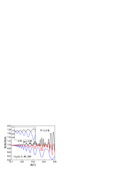
Figure 1: (Color online) Magnetoresistance of the sample A for three different currents $I$ at $T=1.4$ K. The oscillations are inverted with the increase of the current. The inset shows the linear and non-linear (at $I=200$ $\mu$A) magnetoresistance in the low-field region.

The resistance of the sample A as a function of magnetic field at different currents is presented in Figs. 1 and 2. At small currents, the magnetoresistance is positive and modulated by the large-period MIS oscillations clearly visible above $B=0.1$ T. The small-period SdHO, superimposed on the MIS oscillation pattern, appear at higher fields in the low-temperature measurements (Fig. 1). With increasing current $I$, the amplitudes of the MIS oscillations decrease, until a flip of the MIS oscillation picture occurs. This flip, which we associate with inversion of the quantum component of the magnetoresistance from positive to negative, starts from the region of lower fields and extends to higher fields as the current increases. Therefore, one can introduce a characteristic, current-dependent inversion field $B_{inv}$. The inset to Fig. 2 shows the behavior of the magnetoresistance near the point of inversion. In this point, apart from the transition from negative to positive quantum magnetoresistance, we observe an additional feature that looks like splitting of the MIS oscillation peaks or appearance of the next harmonic of the MIS oscillations. This feature persists in higher magnetic fields. In contrast to the MIS oscillations, the SdHO are not inverted by the current, as seen in Fig. 1. However, the SdHO amplitudes decrease as the current increases until the SdHO completely disappear in the low-field region. We attribute this suppression of the SdHO to electron heating at high current densities.

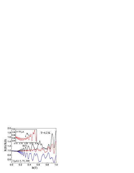
Figure 2: (Color online) Magnetoresistance of the sample A for different currents at $T=4.2$ K. The inset shows inversion of the quantum magnetoresistance around $B=0.2$ T.

The amplitudes of inverted MIS oscillations increase with increasing current and become larger than the MIS oscillation amplitudes in the linear regime. At low temperatures the ratio of the corresponding amplitudes varies between 2 and 3; see Fig. 1. However, when the current increases further, the amplitudes of inverted peaks slowly decrease, this decrease goes faster in the region of lower magnetic fields. This property is seen in Figs. 3 and 4, where the magnetoresistance data for the sample B is presented. The typical current dependence of the inverted peak amplitudes at $T=1.4$ K is shown in the inset to Fig. 3. The behavior of magnetoresistance at 4.2 K, shown in Fig. 4, is similar. In the chosen interval of magnetic fields, the SdHO at 4.2 K are suppressed even in the linear regime. The splitting of the MIS oscillation peaks is clearly visible in Fig. 4 at $I=80$ $\mu$A. For $I=100$ $\mu$A this splitting apparently develops in the frequency doubling of the MIS oscillations. Further increase of the current suppresses this feature, leading to a more simple picture of inverted MIS oscillations.

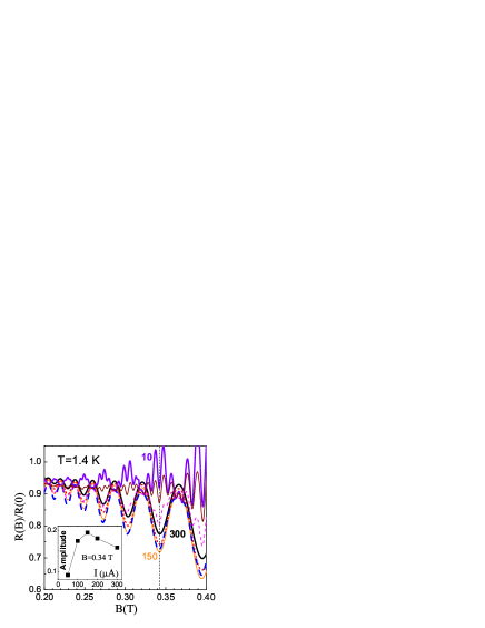
Figure 3: (Color online) Magnetoresistance of the sample B at $T=1.4$ K. The values of the current are 10 (bold), 30, 50 (dash), 100 (bold dash), 150, 200 (short dash), and 300 (bold) $\mu$A. The inset shows amplitudes of the inverted peaks at $B=0.34$ T.

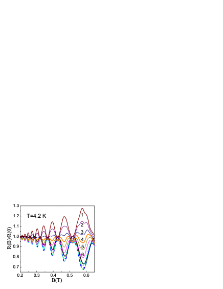
Figure 4: (Color online) Magnetoresistance of the sample B at $T=4.2$ K. The values of the current ($\mu$A) are 1, 50, 80, 100, 120, and 150 for the curves marked by the numbers from 1 to 6, respectively. The other curves corresponds to the currents of 200 (short dash), 250 (bold dash) 300 (solid), 350 (dash), and 400 (bold) $\mu$A.

III Theory

The theoretical interpretation of our data is based on the physical model of Dmitriev et al.,⁷ generalized to the two-subband case. The elastic scattering of electrons is assumed to be much stronger than the inelastic one. This scattering maintains nearly isotropic carrier distribution at moderate currents, when the momentum gained by an electron moving in the electric field between the scattering events is much smaller than the Fermi momentum. Since the intersubband elastic scattering is also much stronger than the inelastic scattering, the isotropic part of electron distribution function, $f_{\varepsilon}$, is common for both subbands and depends only on the electron energy $\varepsilon$. When the current of density $j$ flows through the sample, the kinetic equation for this function is written as

$$\frac{P}{D_{\varepsilon}\sigma_{d}}\frac{\partial}{\partial\varepsilon}\sigma_{d}(\varepsilon)\frac{\partial}{\partial\varepsilon}f_{\varepsilon}=-J_{\varepsilon}(f),$$ (1)

where $P=j^{2}\rho_{d}$ is the power of Joule heating (the energy absorbed per unit time over a unit square of electron system) expressed through the diagonal resistivity $\rho_{d}$, and $D_{\varepsilon}$ is the density of states. The function $\sigma_{d}(\varepsilon)$ can be written through the electron Green’s functions, which are determined by the interaction of electrons with static disorder potential in the presence of magnetic field. The free-electron states in the magnetic field described by the vector potential $(0,Bx,0)$ are characterized by the quantum numbers $j$, $n$, and $p_{y}$, where $j=1,2$ numbers the electron subband of the quantum well, $n$ is the Landau level number, and $p_{y}$ is the continuous momentum. Using the free-electron basis, one obtains

$$\sigma_{d}(\varepsilon)=\frac{e^{2}}{2\pi m}{\rm Re}\left[Q_{\varepsilon}^{AR}-Q_{\varepsilon}^{AA}\right],$$ (2)

$$Q_{\varepsilon}^{ss^{\prime}}=\frac{2\omega_{c}}{L^{2}}\sum_{nn^{\prime}}\sum_{jj^{\prime}}\sqrt{(n+1)(n^{\prime}+1)}\sum_{p_{y}p_{y}^{\prime}}$$

$$\times\left<\left<G^{jj^{\prime},s}_{\varepsilon}(n+1p_{y},n^{\prime}+1p^{\prime}_{y})G^{j^{\prime}j,s^{\prime}}_{\varepsilon}(n^{\prime}p^{\prime}_{y},np_{y})\right>\right>,$$ (3)

where $e$ is the electron charge, $m$ is the effective mass of electron, $G^{jj^{\prime},s}_{\varepsilon}$ are the retarded ($s=R$) and advanced ($s=A$) Green’s functions, and $L^{2}$ is the normalization square. The Zeeman splitting is neglected, so the electrons are assumed to be spin-degenerate. The double angular brackets in Eq. (3) denote averaging over the random potential. In terms of the Green’s functions, the density of states is given by

$$D_{\varepsilon}=\frac{2}{\pi L^{2}}\sum_{jnp_{y}}{\rm Im}\left<\left<G^{jj,A}_{\varepsilon}(np_{y},np_{y})\right>\right>=\frac{2m}{\pi\hbar^{2}}\sum_{j}{\rm Im}S_{j\varepsilon}.$$ (4)

The dimensionless function $S_{j\varepsilon}$ is found from the implicit equation

$$S_{j\varepsilon}=\frac{\hbar\omega_{c}}{2\pi}\sum_{n}\frac{1}{\varepsilon-\hbar\omega_{c}(n+1/2)-\varepsilon_{j}-\Sigma_{j\varepsilon}},$$ (5)

$$\Sigma_{j\varepsilon}=\sum_{j^{\prime}}\frac{\hbar}{\tau_{jj^{\prime}}}S_{j^{\prime}\varepsilon},~{}~{}~{}~{}~{}~{}~{}~{}~{}$$

where $\omega_{c}$ is the cyclotron energy, $\varepsilon_{j}$ is the subband energy, and $\tau_{jj^{\prime}}$ are the quantum lifetimes of electrons with respect to intrasubband ($j^{\prime}=j$) and intersubband ($j^{\prime}\neq j$) scattering. Equation (5) is valid when the correlation length of the disorder potential is smaller than the magnetic length, and the disorder-induced energy broadening of the subbands is smaller than the subband separation $\Delta_{12}=\varepsilon_{2}-\varepsilon_{1}$. It corresponds to the the self-consistent Born approximation (SCBA).

According to the definition (2), the diagonal conductivity is

$$\sigma_{d}=\int d\varepsilon\left(-\frac{\partial f_{\varepsilon}}{\partial\varepsilon}\right)\sigma_{d}(\varepsilon).$$ (6)

Therefore, multiplying the kinetic equation (1) by the density of states $D_{\varepsilon}$ and energy $\varepsilon$, and integrating it over $\varepsilon$, one obtains the balance equation $P=P_{ph}$, where $P_{ph}=-\int d\varepsilon~{}\!\varepsilon D_{\varepsilon}J_{\varepsilon}(f)$ is the power lost to the lattice vibrations (phonons).

Below we consider the case of classically strong magnetic field, $\omega_{c}\tau_{tr}\gg 1$, when $\sigma_{d}(\varepsilon)$ is written in terms of $S_{j\varepsilon}$ as

$$\sigma_{d}(\varepsilon)=\frac{4e^{2}}{m\omega_{c}^{2}}\left[\frac{n_{1}}{\tau^{tr}_{11}}({\rm Im}S_{1\varepsilon})^{2}+\frac{n_{2}}{\tau^{tr}_{22}}({\rm Im}S_{2\varepsilon})^{2}+\frac{n_{s}}{\tau^{tr}_{12}}{\rm Im}S_{1\varepsilon}{\rm Im}S_{2\varepsilon}\right],$$ (7)

where $n_{1}$ and $n_{2}$ are the electron densities in the subbands, $n_{s}=n_{1}+n_{2}$, and $\tau^{tr}_{jj^{\prime}}$ are the transport times of electrons. Both $\tau_{jj^{\prime}}$ and $\tau^{tr}_{jj^{\prime}}$ are determined by the expressions

$$\begin{array}[]{c}1/\tau_{jj^{\prime}}\\ 1/\tau^{tr}_{jj^{\prime}}\end{array}\left\}=\frac{m}{\hbar^{3}}\int_{0}^{2\pi}\frac{d\theta}{2\pi}w_{jj^{\prime}}\left(\sqrt{(k^{2}_{j}+k^{2}_{j^{\prime}})F_{jj^{\prime}}(\theta)}\right)\times\right\{\begin{array}[]{c}1\\ F_{jj^{\prime}}(\theta)\end{array},$$ (8)

where $w_{jj^{\prime}}(q)$ are the Fourier transforms of the correlators of the scattering potential, $F_{jj^{\prime}}(\theta)=1-2k_{j}k_{j^{\prime}}\cos\theta/(k_{j}^{2}+k_{j^{\prime}}^{2})$, and $k_{j}$ is the Fermi wavenumber for the subband $j$. The electron densities in the subbands are expressed as $n_{j}=k^{2}_{j}/2\pi$.

In DQWs, where the energy separation between the subbands is usually small compared to the Fermi energy, the difference $k^{2}_{1}-k^{2}_{2}$ is small in comparison with $k^{2}_{1}+k^{2}_{2}$ so that $n_{1}\simeq n_{2}\simeq n_{s}/2$. Furthermore, in the symmetric (balanced) DQWs, where the electron wave functions are delocalized over the layers and represent themselves symmetric and antisymmetric combinations of single-layer orbitals, one has nearly equal probabilities for intrasubband and intersubband scattering owing to $w_{11}(q)\simeq w_{22}(q)\simeq w_{12}(q)$, provided that interlayer correlation of the scattering potentials is weak. Therefore, $\tau_{jj}\simeq\tau_{12}\simeq 2\tau$, and $\tau^{tr}_{jj}\simeq\tau^{tr}_{12}\simeq 2\tau_{tr}$, where $\tau$ and $\tau_{tr}$ are the averaged quantum lifetime and transport time, respectively. In these approximations, Eq. (7) is written in the most simple way:

$$\sigma_{d}(\varepsilon)\simeq\sigma^{(0)}_{d}{\cal D}^{2}_{\varepsilon},~{}~{}~{}~{}{\cal D}_{\varepsilon}=\frac{1}{2}({\cal D}_{1\varepsilon}+{\cal D}_{2\varepsilon}),~{}~{}~{}~{}{\cal D}_{j\varepsilon}=2{\rm Im}S_{j\varepsilon}$$ (9)

where $\sigma^{(0)}_{d}=\sigma^{2}_{\bot}\rho_{0}$, $\sigma_{\bot}=e^{2}n_{s}/m\omega_{c}$ is the Hall conductivity, and $\rho_{0}=m/e^{2}\tau_{tr}n_{s}$ is the classical resistivity. The function ${\cal D}_{\varepsilon}=1+\gamma_{\varepsilon}$ is the dimensionless density of states, containing oscillating (periodic in $\hbar\omega_{c}$) part $\gamma_{\varepsilon}$. Therefore, it is convenient to solve the kinetic equation by representing the distribution function as a sum $f^{0}_{\varepsilon}+\delta f_{\varepsilon}$, where the first term slowly varies on the scale of cyclotron energy, while the second one rapidly oscillates.⁷ The first term satisfies the equation

$$\kappa\frac{\partial^{2}}{\partial\varepsilon^{2}}f^{0}_{\varepsilon}=-J_{\varepsilon}(f^{0}),~{}~{}~{}\kappa=\frac{\pi\hbar^{2}j^{2}\rho_{0}}{2m}.$$ (10)

Solution of this equation can be satisfactory approximated by a heated Fermi distribution. This is always true if the electron-electron scattering dominates over the electron-phonon scattering and over the electric-field effect described by the left-hand side of Eq. (10). In this case, the Fermi distribution of electrons is maintained against the field-induced diffusion in the energy space, while the electron-phonon scattering determines the effective electron temperature $T_{e}$. In the general case, a numerical solution of Eq. (10) involving electron-phonon scattering in the collision integral¹¹ confirms that $f^{0}_{\varepsilon}$ is very close to the heated Fermi distribution.

The equation for the oscillating part, $\delta f_{\varepsilon}$, is then written in the following form:

$${\cal D}_{\varepsilon}\frac{\partial^{2}}{\partial\varepsilon^{2}}\delta f_{\varepsilon}+2\frac{\partial{\cal D}_{\varepsilon}}{\partial\varepsilon}\frac{\partial}{\partial\varepsilon}\delta f_{\varepsilon}+\kappa^{-1}J_{\varepsilon}(\delta f)=-2\frac{\partial{\cal D}_{\varepsilon}}{\partial\varepsilon}\frac{\partial f^{0}_{\varepsilon}}{\partial\varepsilon}.$$ (11)

Below we search for the function $\delta f_{\varepsilon}$ in the form $\delta f_{\varepsilon}=(\partial f^{0}_{\varepsilon}/\partial\varepsilon)\varphi_{\varepsilon}$, where $\varphi_{\varepsilon}$ is a periodic function of energy. Taking into account that the main mechanism of relaxation of the distribution $\delta f_{\varepsilon}$ is the electron-electron scattering, one may represent the linearized collision integral $J_{\varepsilon}(\delta f)$ as

$$J_{\varepsilon}(\delta f)=-\frac{1}{\tau_{in}}\frac{\partial f^{0}_{\varepsilon}}{\partial\varepsilon}\frac{1}{{\cal N}{\cal D}_{\varepsilon}}\sum_{jj^{\prime}j_{1}j^{\prime}_{1}}M_{jj^{\prime},j_{1}j^{\prime}_{1}}\left<{\cal D}_{j\varepsilon}{\cal D}_{j_{1}\varepsilon+\delta\varepsilon}{\cal D}_{j^{\prime}\varepsilon^{\prime}}{\cal D}_{j^{\prime}_{1}\varepsilon^{\prime}-\delta\varepsilon}\right.$$

$$\left.\times[\varphi_{\varepsilon}+\varphi_{\varepsilon^{\prime}}-\varphi_{\varepsilon+\delta\varepsilon}-\varphi_{\varepsilon^{\prime}-\delta\varepsilon}]\right>_{\varepsilon^{\prime},\delta\varepsilon},~{}~{}~{}~{}{\cal N}=\sum_{jj^{\prime}j_{1}j^{\prime}_{1}}M_{jj^{\prime},j_{1}j^{\prime}_{1}},$$ (12)

where $\delta\varepsilon$ is the energy transferred in electron-electron collisions, $M_{jj^{\prime},j_{1}j^{\prime}_{1}}$ is the probability of scattering (when electrons from the states $j$ and $j^{\prime}$ come to the states $j_{1}$ and $j^{\prime}_{1}$), ${\cal N}$ is the normalization constant, and the angular brackets $\left<\ldots\right>_{\varepsilon^{\prime},\delta\varepsilon}$ denote averaging over the energies $\varepsilon^{\prime}$ and $\delta\varepsilon$. Expression (12) is a straightforward generalization of the result of Ref. 7. The characteristic inelastic scattering time $\tau_{in}$ describes the relaxation at low magnetic fields, when ${\cal D}_{j\varepsilon}$ are close to unity. In this case the collision integral acquires the most simple form $J_{\varepsilon}(\delta f)=-\delta f_{\varepsilon}/\tau_{in}$, i.e. the relaxation time approximation is justified.

The resistivity $\rho_{d}=\sigma^{(0)}_{d}/\sigma^{2}_{\bot}$ is written, according to Eq. (6), in the form

$$\rho_{d}=\rho_{0}\int d\varepsilon{\cal D}^{2}_{\varepsilon}\left(-\frac{\partial f^{0}_{\varepsilon}}{\partial\varepsilon}\right)\left(1+\frac{\partial\varphi_{\varepsilon}}{\partial\varepsilon}\right),$$ (13)

where we have taken into account that $\partial f_{\varepsilon}/\partial\varepsilon\simeq(\partial f^{0}_{\varepsilon}/\partial\varepsilon)\left[1+\partial\varphi_{\varepsilon}/\partial\varepsilon\right]$. Therefore, in order to calculate the resistivity, one should find $\varphi_{\varepsilon}$ by using Eqs. (11) and (12). In general, Eq. (12) is an integro-differential equation that cannot be solved analytically. However, the property of periodicity allows one to expand $\varphi_{\varepsilon}$ in series of harmonics, $\varphi_{\varepsilon}=\sum_{k}\varphi_{k}\exp(2\pi ik\varepsilon/\hbar\omega_{c})$, and represent Eq. (11) as a system of linear equations:

$$(Q^{-1}+k^{2})\varphi_{k}+\sum_{k^{\prime}=-\infty}^{\infty}\left[(2kk^{\prime}-k^{\prime 2})\gamma_{k-k^{\prime}}+Q^{-1}C_{kk^{\prime}}\right]\varphi_{k^{\prime}}=2ik\frac{\hbar\omega_{c}}{2\pi}\gamma_{k},$$ (14)

where

$$Q=\frac{2\pi^{3}j^{2}}{e^{2}n_{s}\omega^{2}_{c}}\frac{\tau_{in}}{\tau_{tr}}$$ (15)

is a dimensionless parameter characterizing the nonlinear effect of the current on the transport. The matrix $C_{kk^{\prime}}$, whose explicit form is not shown here, describes the effects of electron-electron scattering beyond the relaxation time approximation.

The harmonics of the density of states, $\gamma_{k}$, as well as the coefficients $C_{kk^{\prime}}$, which are expressed in terms of products of these harmonics, are proportional to the Dingle factors $\exp(-k\pi/\omega_{c}\tau)$. Therefore, searching for the coefficients $\varphi_{k}$ at weak enough magnetic fields, when $e^{-\pi/\omega_{c}\tau}$ is small, one can take into account only a single ($k=\pm 1$) harmonic. Within this accuracy, one should also neglect the sum in Eq. (14). This leads to a simple solution $\varphi_{\pm 1}=\pm i\gamma_{\pm 1}(\hbar\omega_{c}/\pi)Q/(1+Q)$. Since $\gamma_{+1}+\gamma_{-1}=-2e^{-\pi/\omega_{c}\tau}\cos(\pi\Delta_{12}/\hbar\omega_{c})$, Eq. (13) is reduced to a simple analytical expression for the resistivity:

$$\frac{\rho_{d}}{\rho_{0}}=1+e^{-2\pi/\omega_{c}\tau}\frac{1-3Q}{1+Q}\left(1+\cos\frac{2\pi\Delta_{12}}{\hbar\omega_{c}}\right)$$

$$-4e^{-\pi/\omega_{c}\tau}{\cal T}\cos\left(\frac{2\pi\varepsilon_{F}}{\hbar\omega_{c}}\right)\cos\left(\frac{\pi\Delta_{12}}{\hbar\omega_{c}}\right).$$ (16)

The second term in this expression, proportional to $e^{-2\pi/\omega_{c}\tau}$, differs from a similar term of the single-subband theory⁷ by the modulation factor $\left[1+\cos(2\pi\Delta_{12}/\hbar\omega_{c})\right]/2$ describing the MIS oscillations. The last term in Eq. (16) describes the SdHO, which are thermally suppressed because of the factor ${\cal T}=(2\pi^{2}T_{e}/\hbar\omega_{c})/\sinh(2\pi^{2}T_{e}/\hbar\omega_{c})$. The Fermi energy $\varepsilon_{F}$ is counted from the middle point between the subbands, $(\varepsilon_{1}+\varepsilon_{2})/2$, and, therefore, is directly proportional to the total electron density, $\varepsilon_{F}=\hbar^{2}\pi n_{s}/2m$.

IV Results and discussion

The basic features of our experimental findings can be understood within Eqs. (16) and (15). In the linear regime, when the parameter $Q$ is small, this equation gives a good description of the MIS oscillations experimentally investigated in Ref. 10. As the current increases, the amplitudes of these oscillations decrease, and then the flip occurs, when the MIS peaks become inverted. In contrast, the SdHO peaks are not affected by the the current directly, and their decrease is caused by the effect of heating. The flip of the MIS oscillations corresponds to $Q=1/3$. Since $Q$ is inversely proportional to the square of the magnetic field, there exists the inversion field, $B_{inv}$, determined from the equation $Q=1/3$, where $Q$ is given by Eq. (15). This feature is observed in our experiment, see the inset to Fig. 2. For the sample B, we have extracted $B_{inv}$ for several values of the current. The results are shown in Fig. 5. At 4.2 K the experimental points follow the linear $B_{inv}(I)$ dependence predicted by Eq. (15). Since the ratio $B_{inv}/I$ is proportional to the square root of the inelastic relaxation time $\tau_{in}$, we are able to estimate this time from experimental data as $\tau_{in}\simeq 64$ ps at $T=4.2$ K. Assuming the $T^{-2}$ scaling of this time,⁷ one obtains $\hbar/\tau_{in}=6.6$ mK at $T=1$ K, which is not far than the theoretical estimate $\hbar/\tau_{in}=4$ mK at $T=1$ K based on the consideration of electron-electron scattering.⁷ The positions of experimental points at $T=1.4$ K also fit within this picture if the electron heating is taken into account. The increase of electron temperature with increasing current (heating effect) leads to deviation of the $B_{inv}(I)$ dependence from linearity because of temperature dependence of $\tau_{in}$, and this deviation is essential at $T=1.4$ K; see Fig. 5. The same consideration, applied to the high-mobility sample A, gives the inelastic scattering time $\tau_{in}\simeq 108$ ps at $T=4.2$ K, which is very close to the theoretical estimate.

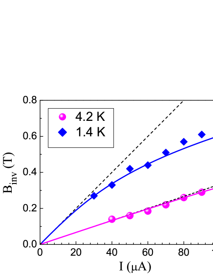
Figure 5: (Color online) Dependence of the inversion field on the current for the sample B at $T=4.2$ K and $T=1.4$ K. (points) The dashed lines correspond to a linear $B_{inv}(I)$ dependence assuming $\tau_{in}=64$ ps at 4.2 K (580 ps at 1.4 K). The solid lines represent the calculated $B_{inv}(I)$ dependence taking into account electron heating by the current.

When the current becomes high enough ($Q\gg 1$), Eq. (16) predicts saturation of the resistance, when the amplitudes of inverted MIS peaks are three times larger than the amplitudes of the MIS peaks in the linear regime ($Q\ll 1$). We indeed observe the regime resembling a saturation, with almost three times increase in the amplitudes of inverted peaks for both samples at $T=1.4$ K (see Figs. 1 and 3). For higher temperatures the behavior is similar, though the maximum amplitudes of inverted peaks are only slightly larger than the amplitudes in the linear regime. We explain this by the effect of heating on the characteristic times. Though the resistivity in the high-current regime ($Q\gg 1$) no longer depends on $\tau_{in}$, there is a sizeable decrease in the quantum lifetime $\tau$ with increasing temperature,¹⁰ which takes place because the electron-electron scattering contributes into $\tau$. As a result, the Dingle factor decreases, and the quantum contribution to the resistance becomes smaller as the electrons are heated. At higher initial temperature, when $\tau_{in}$ is smaller, the regime $Q\gg 1$ requires higher currents. The corresponding increase in heating reduces the quantum contribution, so the maximum amplitudes of inverted peaks never reach the theoretical limit and are expected to decrease with increasing initial temperature. The slow suppression of the inverted peaks with further increase in the current (see the inset to Fig. 3) is explained by the same mechanism. This conclusion is supported by the experimental observation that the suppression is more efficient at lower magnetic fields, when the Dingle factor $\exp(-\pi/\omega_{c}\tau)$ is more sensitive to the temperature dependence of quantum lifetime $\tau$.

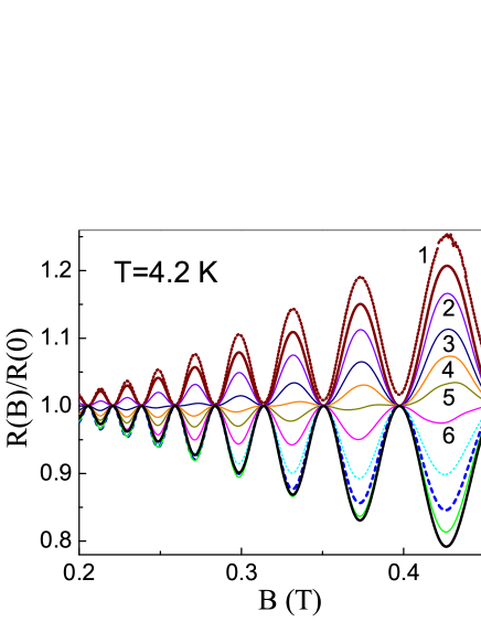
Figure 6: (Color online) Calculated magnetoresistance of the sample B at $T=4.2$ K and different currents: 1, 50, 80, 100, 120, and 150 $\mu$A for the curves marked by the numbers from 1 to 6; the other curves corresponds to $I=200$ (short dash), 250 (bold dash), 300 (solid), and 400 (bold) $\mu$A. The additional (dashed) line 1 shows the linear magnetoresistance determined by the SCBA calculation of the density of states in Eq. (13).

To illustrate the above-discussed relation of the basic theoretical predictions to our experiment, we present the results of theoretical calculations according to Eqs. (15) and (16) in Fig. 6. The calculations are done for the sample B at 4.2 K, so the theoretical curves show the expected behavior of the measured magnetoresistance from Fig. 4. We take into account the effect of heating, described by using the collision integral for interaction of electrons with acoustic phonons¹¹ and temperature dependence of the quantum lifetime $\tau$ of electrons determined empirically from the studies of the MIS oscillations in the linear regime.¹⁰ The theoretical plots demonstrate a reasonable qualitative agreement with the experiment. However, the theory predicts a slower suppression of the inverted peak amplitudes with increasing current at weak magnetic fields. This may be a consequence of underestimated heating,¹² because the screening effect on the electron-phonon interaction¹³ has not been taken into account in the calculation of the power loss to acoustic phonons. Similar calculations carried out for different samples at different temperatures are also in agreement with experimental data.

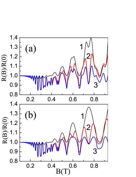
Figure 7: (Color online) (a) Calculated magnetoresistance of the sample B at $T=4.2$ K and $I=120$ $\mu$A. The plot 1 correspond to simple theory [Eq. (16)], while the others represent the results of numerical solution of Eq. (14) for the cases of subband-independent electron-electron scattering (2) and only intrasubband electron-electron scattering (3). (b) The same plots, where the SdHO contribution is excluded. The density of states is found within the SCBA.

The simple theory fails do describe the interesting and unexpected feature observed in our experiment, the current-induced splitting of the MIS oscillation peaks. This kind of nonlinear behavior is well-reproducible, we see it in different samples. We have found that a possible explanation of this feature can be based on the theory presented in Sec. III, if higher harmonics of the distribution function $\delta f_{\varepsilon}$ are taken into account. We have carried out a numerical solution of the system of equations (14) under some simplifying assumptions about the collision integral. In the first case, we have assumed equal probabilities for all possible electron-electron scattering processes, so the matrix $M_{jj^{\prime},j_{1}j^{\prime}_{1}}$ in Eq. (12) is replaced by a constant. Another limiting case we consider is the complete neglect of intersubband transitions in electron-electron collisions, when $M_{jj^{\prime},j_{1}j^{\prime}_{1}}\propto\delta_{jj_{1}}\delta_{j^{\prime}j^{\prime}_{1}}$. This case is also reasonable, since electron-electron scattering at low temperatures assumes a small momentum transfer, so the intersubband scattering contribution should be suppressed owing to reduction of the overlap integrals of envelope wave functions of electrons. Then, the coefficients $\gamma_{k}$ and $C_{kk^{\prime}}$ have been determined by using the density of states numerically calculated within the SCBA; see Eq. (5). The results, corresponding to $I=120$ $\mu$A for the sample B are presented in Fig. 7. In the low-field region, where the MIS peaks are inverted, the calculation shows a considerable increase in their amplitudes above 0.2 T, where contribution of higher harmonics of the density of states becomes essential. This enhancement occurs because of the current-induced mixing between different harmonics of the distribution function, formally coming from the term with $\gamma_{k-k^{\prime}}$ in the sum in Eq. (14). In contrast, in the linear regime, the SCBA magnetoresistance is close to the magnetoresistance calculated within the single-harmonic approximation [Eq. (16)]; see Fig. 6. Above 0.27 T, where the Landau levels become separated, one can see features associated with the specific semi-elliptic shape of the SCBA density of states. In the vicinity of the inversion field ($B_{inv}\simeq 0.4$ T), where the contribution of the first harmonic of the distribution function is suppressed ($Q\simeq 1/3$) while the higher harmonics are still active, two sets of MIS peaks are seen. It is not surprising, because higher harmonics of the density of states contain the factors $\cos(k\pi\Delta_{12}/\hbar\omega_{c})$ describing higher harmonics of the MIS oscillations. Above the inversion field, the resistance is considerably smaller than the resistance predicted by the single-harmonic approximation, and a splitting of the MIS peaks occurs. The splitting increases with the increase of the magnetic field. These effects are caused by the contribution of higher harmonics of the density of states in the collision integral. Indeed, in the single-harmonic approximation the collision integral contains only the outcoming term proportional to $\varphi_{\varepsilon}$. This approximation becomes insufficient in higher magnetic fields, when incoming terms in the collision integral (12) are also important, so the relaxation of the distribution function, which counteracts the diffusion of electrons in the energy space, becomes less efficient. This means that the effect of the current on the distribution function increases, and the resistance is lowered. The described suppression of the collision-integral term is more significant in the regions of the MIS resonances, when $\Delta_{12}/\hbar\omega$ is integer, because the peaks of the density of states are the narrowest in these conditions, and the energies transferred in the electron-electron collisions, $\delta\varepsilon$, are small. Away from the MIS resonances, the energy space for electron-electron scattering increases, especially when the intersubband transitions are allowed (see curve 2 in Fig. 7). Therefore, the relaxation is less suppressed as compared to the center of the MIS peak, and the effect of the current is weaker. The above consideration explains why the centers of the MIS peaks drop down, so the peak splitting takes place.

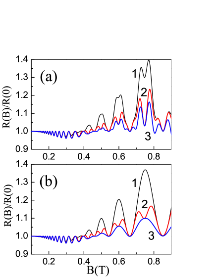
Figure 8: (Color online) The same as in Fig. 7 for the Gaussian model of the density of states.

The SCBA has a limited applicability for description of the density of electron states in the magnetic field. In particular, it leads to non-physically sharp edges of the density of states, which generate the harmonics $\gamma_{k}$ with large $k$ in Eq. (14). This apparently leads to an overestimate of the effect of the current on the resistance in the region where the MIS peaks are inverted, see Fig. 7. To avoid such singularities, and to have a further insight into the problem of nonlinear magnetoresistance, we have considered the expression

$${\cal D}^{(G)}_{1,2\varepsilon}=\frac{\hbar\omega_{c}}{\sqrt{\pi}\Gamma(\omega_{c})}\sum_{n=-\infty}^{\infty}\exp\frac{[\varepsilon\pm\Delta_{12}/2-\hbar\omega_{c}(n+1/2)]^{2}}{\Gamma^{2}(\omega_{c})}.$$ (17)

which corresponds to the Gaussian model for the density of states and describes two independent sets of Landau-level peaks from each subband (strictly speaking, the Landau-level peaks are not independent because of elastic intersubband scattering, as follows from Eq. (5), see more details in Ref. 14). The magnetic-field dependence of the broadening energy $\Gamma$ has been set to make the first [proportional to $\cos(2\pi\varepsilon/\hbar\omega_{c})$] harmonics of ${\cal D}^{(G)}_{j\varepsilon}$ and ${\cal D}_{j\varepsilon}$ equal. The results of the calculations using ${\cal D}^{(G)}_{j\varepsilon}$ instead of the SCBA density of states are shown in Fig. 8. The magnetoresistance in the region of inversion appears to be nearly the same as predicted by the simple single-harmonic theory. In the region above the inversion field, the splitting of the MIS peaks does not take place if the intersubband electron-electron scattering is forbidden. This is understandable from the discussion given above: if different subbands contribute into the density of states independently, the efficiency of electron-electron collisions does not depend on the ratio $\Delta_{12}/\hbar\omega$ and the reduction of the collision integral owing to incoming terms causes just a uniform suppression of the whole MIS peak. In the SCBA, when the shape of ${\cal D}_{j\varepsilon}$ depends on this ratio, the splitting of the MIS peaks does not necessarily require the intersubband electron-electron scattering.

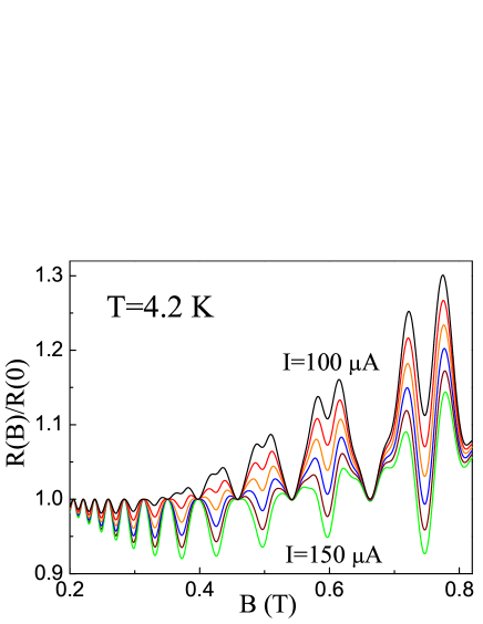
Figure 9: (Color online) Evolution of the nonlinear magnetoresistance calculated using the parameters of the sample B when the current varies from 100 to 150 $\mu$A with the step of 10 $\mu$A. The Gaussian model of the density of states and the assumption of subband-independent electron-electron scattering are used.

If the intersubband electron-electron scattering is allowed, the magnetoresistance pictures obtained within the Gaussian model, as well as within the SCBA model above the inversion point, qualitatively reproduce the features we observe experimentally. The results of calculations presented in Fig. 9 demonstrate that varying the current in a relatively narrow range leads to a dramatic reconstruction of the magnetoresistance oscillation pattern.

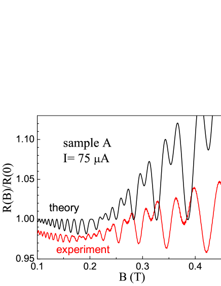
Figure 10: (Color online) Comparison of the measured and calculated nonlinear magnetoresistance in the sample A at $T=4.2$ K and $I=75$ $\mu$A. The Gaussian model of the density of states and the assumption of subband-independent electron-electron scattering are used in the calculations.

Numerical calculation of magnetoresistance in the high-mobility sample A also gives the results very similar to what we see experimentally. To demonstrate this, we have put experimental and calculated curves together in Fig. 10. Apart from a weak negative magnetoresistance at low fields and a slight decrease in the MIS oscillations frequency with increasing $B$ (the features we see in all our samples^10,15 both in linear and nonlinear regimes), the agreement between experiment and theory is good.

V Conclusions

Investigation of nonlinear transport of 2D electrons in magnetic fields enriches the knowledge of the quantum kinetic properties of electron systems and of the microscopic processes responsible for the observed modifications of the resistivity. In our work, we have demonstrated that using double quantum well systems opens wide possibilities for studying the nonlinear behavior. The presence of the MIS oscillations, which modulate the quantum component of the resistivity, allows us to investigate the current dependence of the quantum magnetoresistance. In particular, we are able to determine the magnetic fields $B_{inv}$ corresponding to the current-induced inversion of the magnetoresistance. This inversion manifests itself in a spectacular way, as a flip of the MIS oscillation pattern. We point out that this behavior resembles recently observed¹⁵ inversion of the MIS oscillations by the low-frequency (35 GHz) microwave radiation. This is not surprising, because the physical mechanism in both cases is similar. Apart from the flip of the MIS oscillations, we have observed a wholly unexpected quantum phenomenon, the splitting of the MIS oscillation peaks in the region of fields above the inversion point $B_{inv}$.

We have shown that the theoretical explanation of all the observed phenomena can be based on the kinetic equation for the isotropic non-equilibrium part of electron distribution function. This function oscillates with energy owing to oscillations of the density of electron states in the magnetic field. The effect of electric current on this function, the increase of electron diffusion in the energy space, is equilibrated by the inelastic electron-electron scattering. Theoretical explanation of the most of observed phenomena is done in a simple single-harmonic approach, which allowed us to determine the inelastic relaxation time $\tau_{in}$ by comparison of experimental data with theory. The values of $\tau_{in}$ for different samples are close to the theoretical estimates of this time, and confirm the predicted⁷ temperature dependence $\tau_{in}\propto T^{-2}$. Thus, our data on the inelastic relaxation time in double quantum well samples are in agreement with the data obtained in single quantum well samples.⁵ The description of the splitting of MIS oscillations requires a more detailed numerical analysis including consideration of higher harmonics of both the density of states and the distribution function. Apart from the verification of the basic principles of the theory of Ref. 7, this analysis demonstrates sensitivity of the nonlinear behavior to the shape of the density of electron states and to the details in description of inelastic scattering. Therefore, investigation of nonlinear magnetoresistance in relatively weak magnetic fields offers a tool for studying the electron states and scattering mechanisms both in single and double quantum wells.

This work was supported by CNPq and FAPESP (Brazilian agencies).

References

- (1) G. Ebert, K. von Klitzing, K. Ploog, and G. Weimann, J. Phys. C 16, 5441 (1983); M. E. Cage, R. F. Dziuba, B. F. Field, E. R. Williams, S. M. Girvin, A. C. Gossard, D. C. Tsui, and R. J. Wagner, Phys. Rev. Lett. 51, 1374 (1983).
- (2) C. L. Yang, J. Zhang, R. R. Du, J. A. Simmons, and J. L. Reno, Phys. Rev. Lett. 89, 076801, (2002).
- (3) W. Zhang, H. S. Chiang, M. A. Zudov, L. N. Pfeiffer, and K. W. West, Phys. Rev. B 75, 041304(R) (2007).
- (4) A. A. Bykov, J. Q. Zhang, S. Vitkalov, A. K. Kalagin, and A. K. Bakarov, Phys. Rev. B 72, 245307 (2005).
- (5) J.-q. Zhang, S. Vitkalov, A. A. Bykov, A. K. Kalagin, and A. K. Bakarov, Phys. Rev. B 75, 081305(R) (2007).
- (6) X. L. Lei, Appl. Phys. Lett. 90, 132119 (2007)
- (7) I. A. Dmitriev, M. G. Vavilov, I. L. Aleiner, A. D. Mirlin, and D. G. Polyakov, Phys. Rev. B 71, 115316 (2005).
- (8) M. G. Vavilov, I. L. Aleiner, and L. I. Glazman, Phys. Rev. B 76, 115331 (2007).
- (9) M. G. Vavilov and I. L. Aleiner, Phys. Rev. B 69, 035303 (2004).
- (10) N. C. Mamani, G. M. Gusev, T. E. Lamas, A. K. Bakarov, and O. E. Raichev, Phys. Rev. B 77, 205327 (2008).
- (11) See, for example, O. E. Raichev and F. T. Vasko, Phys. Rev. B 74, 075309 (2006).
- (12) According to our calculations, application of the current of 400 A to the sample B at 4.2 K increases electron temperature to 6.3 K.
- (13) Y. Ma, R. Fletcher, E. Zaremba, M. D’Iorio, C. T. Foxon, and J. J. Harris, Phys. Rev. B 43, 9033 (1991).
- (14) O. E. Raichev, Phys. Rev. B 59, 3015 (1999).
- (15) S. Wiedmann, G. M. Gusev, O. E. Raichev, T. E. Lamas, A. K. Bakarov, and J. C. Portal, Phys. Rev. B 78, 121301 (2008).