Implementation of on-site velocity boundary conditions for D3Q19 lattice Boltzmann

Abstract

On-site boundary conditions are often desired for lattice Boltzmann simulations of fluid flow in complex geometries such as porous media or microfluidic devices. The possibility to specify the exact position of the boundary, independent of other simulation parameters, simplifies the analysis of the system. For practical applications it should allow to freely specify the direction of the flux, and it should be straight forward to implement in three dimensions. Furthermore, especially for parallelized solvers it is of great advantage if the boundary condition can be applied locally, involving only information available on the current lattice site. We meet this need by describing in detail how to transfer the approach suggested by Zou and He Zou and He (1997) to a D3Q19 lattice. The boundary condition acts locally, is independent of the details of the relaxation process during collision and contains no artificial slip. In particular, the case of an on-site no-slip boundary condition is naturally included. We test the boundary condition in several setups and confirm that it is capable to accurately model the velocity field up to second order and does not contain any numerical slip.

I Introduction

The lattice Boltzmann method (LBM) is a widely used method for the simulation of fluid flow Succi (2001). It solves the Boltzmann equation on a discrete lattice and it has been proven that the Navier Stokes equations can be recovered Chen et al. (1992); Higuera et al. (1989). The method has been successfully applied to the simulation of flow in porous media Kutay et al. (2006); Martys and Chen (1996), colloidal suspensions Ladd (1994a, b); Ladd and Verberg (2001); Harting et al. (2008), liquid-gas phase transitions and multi-component flows Shan and Chen (1993, 1994); Chen et al. (2000), spinodal decomposition Harting et al. (2005); Chin and Coveney (2002), and many more applications.

In spite of the wide range of applications of the LBM there is sitll little consensus on how to implement boundary conditions in the LBM. For some applications, especially for complex geometries in technical applications, rather simple approaches like on-site bounce back Frisch et al. (1987) rules are preferred Ginzburg and Steiner (2003), and on the other hand quite complex methods to implement exact boundary conditions have been proposed Skordos (1993); Ginzbourg and d’Humières (1996). A promising approach of velocity boundary conditions by Zou and He Zou and He (1997) for 2D simulations has been generalized to 3D with the restriction to the inflow being perpendicular to the boundary plane by Kutay et al.  Kutay et al. (2006). However, to our knowledge, a generalization to 3D with variable inflow direction has not yet been presented. Apart from this restriction, in the terms used in LABEL:Kutay06 some of the prefactors have to be revised (the correct ones can be found in LABEL:Mattila09), but for the application studied by Kutay et al. , the terms used in their work might be appropriate. However, especially if the influx direction is not aligned with the computational lattice, our slightly more general expressions have to be used. We follow the ideas of Zou and He Zou and He (1997) and derive flux boundary conditions with variable influx direction for a D3Q19-lattice Qian (1997) meaning that in three dimensions the velocity space contains 19 discrete vectors. Zou and He Zou and He (1997) have demonstrated a derivation for the D2Q9 model and shortly sketched the application to pressure boundaries in a D3Q15i model, where i stands for an incompressible model of equilibrium distribution functions Zou et al. (1995). Already Zou and He point out that besides the basic idea of applying a bounce back rule to the non-equilibrium part, a further modification is necessary to achieve the correct transversal momentum. A suitable choice for this correction depends on the lattice type. Zou and He give an expression for the D3Q15i lattice for the case of pressure boundaries. In the subsequent publications on D3Q19 lattices Kutay et al. (2006); Mattila et al. (2009), which is one of the most commonly used lattice types nowadays, it is assumed that the flux direction is restricted to the direction normal to the boundary plane and that this symmetry is also reflected in the distribution functions on the boundary nodes. In our generalization we drop this restriction and consistently derive the transversal momentum corrections. We investigate the accuracy of this boundary condition and highlight the special case of on-site no-slip boundary conditions included in this approach by simply setting the velocity equal to zero.

Examples for possible applications are microfluidic devices Karniadakis et al. (2005), i.e., microscopic channel structures which are specially designed to modify a given flow profile by the roughness or wettability of the walls or the geometry of the channels. One example for those structures are micromixers Hessel et al. (2005). In general, if simulating such devices, it is not always possible to align all walls with the Cartesian planes. In these cases one needs a boundary condition which is capable to specify the velocity in an arbitrary direction, depending on the orientation of the channel to be simulated.

One might also think of applications in porous media Kutay et al. (2006), where flow through discretized samples of stones are simulated. On the boundaries of the microscopic pores, a no-slip condition has to be applied. This is a special case of velocity boundary conditions with the velocity being zero. Since the channels cannot be aligned with the computational lattice, the question raises, how large the error introduced by the discretization is. The on-site velocity boundary conditions brought forward in the present paper can be used as a replacement of the bounce-back rule for the no-slip condition if the velocity is set to zero. In contrast to the usual bounce-back rule the position of the wall is independent of the BGK relaxation time. This fact is of great advantage when analyzing the permeability of a discretized sample.

Although the assumption of the fluid velocity being zero on the boundaries does not hold for several cases in microfluidics, the no-slip condition is highly important for many cases. Therefore, a considerable effort of research has been spent to develop no-slip boundary conditionsInamuro et al. (1995); Maier et al. (1996); Ginzbourg and d’Humières (1996); Succi (2001). Some approaches turned out to contain an artificial slip length depending on various details of the simulation method, whereas other attempts involve non-local calculations like the evaluation of a velocity gradient to extrapolate the flow field beyond the boundary. In contrast to that, the boundary condition we propose is of local type and allows to specify the velocity on the node exactly with vanishing slip length.

Further, the boundary condition is of great benefit for hybrid simulations, i.e., simulations in which two simulation methods are coupled to simulate fluid flow Flekkøy et al. (2000); Delgado-Buscalioni and Coveney (2003); Delgado-Buscalioni et al. (2008). The main goal of such hybrid simulations is to save computing time. A computationally cheap method is applied to simulate the flow on a more coarse-grained level, whereas in some regions, where for example interactions on the atomistic level are relevant, a different simulation method comprising more details is applied. The two simulation methods are coupled for example by exchange of mass, momentum and energy between the two domains via their respective boundary conditions. One can think of different setups: an LB simulation can be embedded into a finite element based Navier Stokes solver and resolve one region in more detail. Another example case is that in an LB simulation one region is resolved even on the molecular level by means of a Molecular Dynamics simulation. Practically, in current hybrid simulations the coupling is implemented within an overlapping region Dupuis et al. (2007) of the two simulations, but it would be a great advance if one could manage simply to couple two boundary conditions without any overlap being needed. The possibility to generally determine the velocity on a boundary node in an LB simulation is one step towards this goal.

The remainder of this paper is structured as follows: in the following section we describe the simulation method in general and introduce our notation of the lattice vectors. Then, we shortly review different boundary conditions in the literature in Sec. III. After that, we derive and discuss the velocity boundary condition for the D3Q19 lattice in Sec. IV. We separately discuss the special case of the no-slip condition in Sec. V. Numerical results are presented and discussed in Sec. VI and finally, we draw a conclusion in the closing section of the current paper.

II Simulation method

The lattice Boltzmann method is a numerical method to solve the Boltzmann equation Eq. (1) on a discrete lattice. The Boltzmann equation describes the dynamics of a gas from a microscopic point of view: in a gas, particles, each with velocities $\mathbf{v}_{i}$, collide with a certain probability and exchange momentum among each other. For ideal collisions total momentum and energy are conserved in the collisions. The Boltzmann equation expresses how the probability $f(\mathbf{x},\mathbf{v},t)$ of finding a particle with velocity $\mathbf{v}$ at a position $\mathbf{x}$ and at time $t$ evolves with time:

$$\mathbf{v}\cdot\nabla_{\mathbf{x}}f+\mathbf{F}\cdot\nabla_{\mathbf{p}}f+\frac{\partial f}{\partial t}=\hat{\Omega}(f)\,,$$ (1)

where $\mathbf{F}$ denotes an external body force, $\nabla_{\mathbf{x},\mathbf{p}}$ the gradient in position and momentum space, and $\hat{\Omega}(f)$ denotes the collision-operator. Bhatnagar, Gross, and Krook Bhatnagar et al. (1954) proposed the so-called BGK dynamics, where the collision operator $\hat{\Omega}$ is chosen as a relaxation with a characteristic time $\tau$ to the equilibrium distribution $f^{(eq)}(\mathbf{v},\rho)$.

$$\hat{\Omega}(f)=-\frac{1}{\tau}\left(f-f^{(eq)}\right)\,.$$ (2)

The equilibrium distribution function for athermal models depends on the local density $\rho(\mathbf{x},t)$ and the velocity field $\mathbf{v}(\mathbf{x},t)$. The lattice Boltzmann method McNamara and Zanetti (1988) discretizes the probability density $f$ in space and time. The discrete Boltzmann equation, which is solved by the LBM can be rigorously derived from the Boltzmann equation He and Luo (1997). The discretization, and especially the analytic expression for the equilibrium distribution $f^{(eq)}$ depends on the lattice type. We use a D3Q19-lattice which is a very popular lattice type for 3D LB-simulations. On each lattice site 19 values $f_{i}({\mathbf{x}},t)$ are stored, each of them assigned to a lattice vector $\mathbf{c}_{i}$. We use the notation that the vectors $\mathbf{c}_{i}$ are the $i^{th}$ column vector of the matrix

$$\mathbf{M}=\left[\,\begin{array}[]{ccccccccccccccccccc}\,1&\,-1&\,0&\,0&\,0&\,0&\,1&\,1&\,1&\,1&\,-1&\,-1&\,-1&\,-1&\,0&\,0&\,0&\,0&\,0\\ \,0&\,0&\,1&\,-1&\,0&\,0&\,1&\,-1&\,0&\,0&\,1&\,-1&\,0&\,0&\,1&\,1&\,-1&\,-1&\,0\\ \,0&\,0&\,0&\,0&\,1&\,-1&\,0&\,0&\,1&\,-1&\,0&\,0&\,1&\,-1&\,1&\,-1&\,1&\,-1&\,0\\ \end{array}\,\right]\,.$$ (3)

The geometry is shown in Fig. 1 .

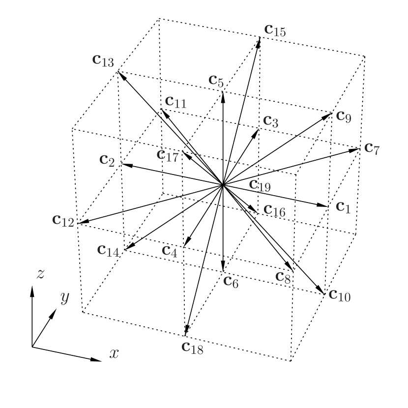
Figure 1: The geometry of the D3Q19 lattice with lattice vectors $\mathbf{c}_{i}$ as defined in Eq. (3).

The local density at a lattice point can be obtained by summing up all $f_{i}$,

$$\rho(\mathbf{x},t)=\sum\limits_{i=1}^{19}f_{i}(\mathbf{x},t)\,,$$ (4)

and the streaming velocity is given by

$$\mathbf{v}(\mathbf{x},t)=\frac{1}{\rho(\mathbf{x},t)}\sum\limits_{i=1}^{19}f_{i}(\mathbf{x},t)\mathbf{c}_{i}\,.$$ (5)

We express all quantities in lattice units, i.e., time is measured in units of update intervals and length is measured in units of the lattice constant. For practical applications a suitable mapping to physical units based on a dimensional analysis has to be applied.

In the lattice Boltzmann method two steps are performed in an alternating way:

1. The “streaming step”: propagate each of the distribution functions $f_{i}$ to the next lattice site in the direction of its assigned lattice vector $\mathbf{c}_{i}$ .

2. The “collision step”: on each lattice site relax the probability functions $f_{i}$ towards the equilibrium value $f_{i}^{(eq)}(\mathbf{v},\rho)$. In BGK dynamics this is according to Eq. (2).

The equilibrium value $f_{i}^{(eq)}$ is obtained by discretizing the Boltzmann distribution. Several expressions of different order have been proposed, where we use the popular form involving terms in the velocity up to the second order Qian et al. (1992); Tang et al. (2005); Zou and He (1997); Sbragaglia and Succi (2005); Chen et al. (1996)

$$f_{i}^{(eq)}(\rho,\mathbf{v})=w_{i}\rho\left[1+\frac{\mathbf{c}_{i}\cdot\mathbf{v}}{c_{s}^{2}}+\frac{(\mathbf{c}_{i}\cdot\mathbf{v})^{2}}{2c_{s}^{4}}-\frac{v^{2}}{2c_{s}^{2}}\right]$$ (6)

with the lattice speed of sound $c_{s}=\frac{1}{\sqrt{3}}$ for the D3Q19 lattice and the lattice weights

$$w_{i}=\left\{\begin{array}[]{rcl}\frac{2}{36},&&i=1\dots 6\\ &&\\ \frac{1}{36},&&i=7\dots 18\\ &&\\ \frac{12}{36},&&i=19\end{array}\right.$$ (7)

The pressure $p=c_{s}^{2}\rho$ turns out to be proportional to the density and the dynamic shear viscosity is given by Hänel (2004); Succi (2001)

$$\eta=c_{s}^{2}\rho\left(\tau-\frac{1}{2}\right)\,.$$ (8)

III Boundary conditions

On the boundary nodes, the distribution function assigned to vectors $\mathbf{c}_{i}$ pointing out of the lattice move out of the computational domain in the propagation step, and the ones assigned to the opposing vectors are undetermined because there are no nodes which the distributions could come from. Therefore, on the boundary nodes, special rules have to be applied.

These boundary conditions can be chosen in various manners. Periodic boundaries are realized by propagating the $f_{i}$ leaving the computational domain on the one boundary to the boundary nodes located on the opposite side of the domain. Closed boundaries are commonly implemented by a so-called mid-grid bounce-back rule Succi (2001), which means that the distributions $f_{i}$ pointing out of the domain are copied to $f_{j}$, for which $\mathbf{c}_{j}=-\mathbf{c}_{i}$, i.e., locally, on each lattice site, the undetermined values are filled with the ones which would stream out of the domain without collision on the boundary node. They enter one time step later into the simulation domain again Sukop and Thorne (2007).

However, for many questions in fluid dynamics it is required to determine the pressure or the velocity field at the boundary. The first is known as Dirichlet boundary condition, and the latter as Neumann boundary condition. In the Neumann case the flux on the boundary of the domain is fixed, whereas in the Dirichlet case the pressure is given as a boundary condition.

Zou and He Zou and He (1997) have proposed how to implement Dirichlet and Neumann boundary conditions on a D2Q9 lattice and shortly sketched how to apply it for a D3Q15i simulation. Kutay et al.  Kutay et al. (2006) have transferred this proposal to a D3Q19 lattice. However, their approach is derived under the assumption that the in- and outflow velocity is always perpendicular to the boundary plane, and oriented along one of the main lattice directions ($\mathbf{c}_{i},\ i=1\dots 6$). We generalize this to inflow with arbitrary direction in Sec. IV.

Often more elaborated boundary conditions are applied. Chen and co-workers Chen et al. (1996) and Ginzbourg and d’Humières Ginzbourg and d’Humières (1996) suggested extrapolation of the $f_{i}$ on the first and second layer of the lattice to the nodes outside the domain. These extrapolated values can be thought of as the lattice populations propagating into the domain and arriving on the boundary nodes in the next streaming step. Inamuro and co-workers have introduced a counter-slip to compensate a numerical slip which occurs when applying on-site bounce-back Inamuro et al. (1995). Skordos came up with an approach where additional differential equations are solved on the boundary nodes to calculate the unknown populations Skordos (1993). Ansumali and Karlin have developed a LB no-slip boundary condition from kinetic theory Ansumali and Karlin (2002), and, more recently, d’Orazio et al.  d’Orazio et al. (2003) and Tang et al.  Tang et al. (2005) came up with thermal boundary conditions which also involve an extrapolation scheme and bounce-back with counter-slip respectively. Ladd and Verberg have developed a boundary condition with a resolution of the position of the wall on a sub-grid level, which is especially required if suspended particles are modeled Ladd and Verberg (2001); Verberg and Ladd (2001); Chun and Ladd (2007). Schiller and Dünweg Schiller (2008) use a reduced set of distribution functions on the boundary nodes. For their reduced D3Q19 model they derive equilibrium distributions and propose a multi relaxation time dynamics and a special collision operator on the boundary.

Latt et al. have compared and discussed several of these approaches in LABEL:Latt08. They also include the boundary condition by Zou and He Zou and He (1997) in their discussion. As indicated by Latt et al. a generalization of the boundary conditions proposed by Zou and He is still not provided. However, a general local boundary rule which can be applied in a simple way on each node separately, would be desirable.

We derive such a boundary condition in the following section. Our generalization of the velocity boundary condition proposed in LABEL:ZouHe only involves the distribution functions defined on the local boundary node and allows by very simple and computationally cheap steps to set the velocity on the node to a distinct vector. The desired value is obtained exactly and we cannot detect any artifacts like a numerical slip length or bends in the velocity profile.

IV General on-site velocity boundary condition

As mentioned in the previous section, we extend the boundary condition by Zou and He Zou and He (1997) to a D3Q19 lattice. We derive the boundary condition for the bottom plane ($z=0$) in detail and give the results for the other planes in the appendix. They can be derived following the same steps.

The boundary conditions are derived by using the set of equations consisting of Eq. (4) and the components of Eq. (5):

$$\rho v_{x} = f_{1}+f_{7}+f_{8}+f_{9}+f_{10}$$ (9)

$$-(f_{2}+f_{11}+f_{12}+f_{13}+f_{14})\,,$$

$$\rho v_{y} = f_{3}+f_{7}+f_{11}+f_{15}+f_{16}$$ (10)

$$-(f_{4}+f_{8}+f_{12}+f_{17}+f_{18})\,,$$

$$\rho v_{z} = f_{5}+f_{9}+f_{13}+f_{15}+f_{17}$$ (11)

$$-(f_{6}+f_{10}+f_{14}+f_{16}+f_{18})\,.$$

Due to the continuity relation $\frac{\partial\rho}{\partial t}+\nabla\cdot(\rho\mathbf{v})=0$, we are free to specify only three of the four variables ($\rho$ and the three components of $\mathbf{v}$) on the boundary. If we fix the tangential velocity $v_{x},v_{y}$ on the bottom-layer of the lattice, and the density to a given value $\rho_{0}$, the $z$-component of the inflow velocity $v_{z}$ can be calculated from Eq. (11) and Eq. (4),

$$v_{z}=1 - \frac{1}{\rho_{0}}\left[f_{1}+f_{2}+f_{3}+f_{4}\right.$$

$$+ f_{7}+f_{8}+f_{11}+f_{12}+f_{19}$$

$$+ \left.2(f_{6}+f_{10}+f_{14}+f_{16}+f_{18})\right]\,,$$

where the $f_{i}$ pointing out of the system appear with a prefactor of $2$, and all in-plane components appear with weight $1$. The components pointing into the system, $f_{5},f_{9},f_{13},f_{15},$ and $f_{17}$, which are undetermined after the streaming step, do not appear at all. With Eq. (IV) Neumann (or pressure) boundary conditions can be applied by specifying $\rho_{0}$ on the boundary and using Eq. (IV) to calculate $v_{z}$. If Eq. (IV) is written in the form

$$\rho = \frac{1}{1-v_{z}}\left[f_{1}+f_{2}+f_{3}+f_{4}\right.$$

$$+ f_{7}+f_{8}+f_{11}+f_{12}+f_{19}$$

$$+ \left.2(f_{6}+f_{10}+f_{14}+f_{16}+f_{18})\right]\,,$$

all three components of the velocity can be specified and Eq. (IV) is used to calculate the density $\rho$. This is the Dirichlet case, or flux-boundary condition. Again, the undetermined populations $f_{5},f_{9},f_{13},f_{15},$ and $f_{17}$ do not enter the calculation.

We have used two out of four equations (Eqns. (9)–(11) and Eq. (4)), but we still have to compute the five $f_{i}$ pointing into the computing domain. Following Zou and He Zou and He (1997) we assume that on the boundary the bounce-back condition is still valid for the non-equilibrium part $f_{i}^{*}$ of the single particle distribution $f_{i}$:

$$f_{i}^{*}=f_{i}-f_{i}^{(eq)}\,.$$ (14)

The bounce-back condition in $+z$-direction (in normal direction to the boundary) would read as

$$f_{5}^{*}=f_{5}-f_{5}^{(eq)}=f_{6}-f_{6}^{(eq)}=f_{6}^{*}\,,$$ (15)

which leads by taking $f_{5}^{(eq)}$ and $f_{6}^{(eq)}$ from Eq. (14) to

$$f_{5} = f_{6}-w_{6}\rho\left[1-\frac{v_{z}}{c_{s}^{2}}+\frac{v_{z}^{2}}{2c_{s}^{4}}\right]$$ (16)

$$\phantom{f_{6}}+w_{5}\rho\left[1+\frac{v_{z}}{c_{s}^{2}}+\frac{v_{z}^{2}}{2c_{s}^{4}}\right]$$

$$= f_{6}+\frac{2w_{5}}{c_{s}^{2}}\rho v_{z}=f_{6}+\frac{1}{3}\rho v_{z}\,.$$

Here we make use of the fact that the distribution functions in Eq. (6) are approximated by taking only terms up to $2^{nd}$ order in $\mathbf{v}$ into account. However, this approximation could be applied directly to Eq. (16) as well. For the derivation of the boundary condition it is needed, otherwise the higher order terms would introduce anisotropic effects in the boundary rule.

Generally, in the collision step (in Eq. (2)) higher order terms may be taken into account for the bulk, but for the boundary conditions a qualitatively different approach, like a higher order extrapolation scheme, has to be considered when aiming for higher order accuracy.

For the D3Q19 lattice, however, we need two more equations. To keep the symmetry of the problem, we assume bounce-back of the non-equilibrium part for all populations $f_{i}$. This results in four equations,

$$f_{9} = f_{14}+\frac{2w_{9}}{c_{s}^{2}}\rho(v_{z}+v_{x})\,,$$ (17)

$$f_{13} = f_{10}+\frac{2w_{13}}{c_{s}^{2}}\rho(v_{z}-v_{x})\,,$$ (18)

$$f_{15} = f_{18}+\frac{2w_{15}}{c_{s}^{2}}\rho(v_{z}+v_{y})\,,$$ (19)

$$f_{17} = f_{16}+\frac{2w_{17}}{c_{s}^{2}}\rho(v_{z}-v_{y})\,,$$ (20)

so that the system of equations is overdetermined.

Therefore, following the Ansatz by Zou and He Zou and He (1997) for the pressure boundary condition on a D3Q15i lattice, we introduce two new variables $N^{z}_{x}$ and $N^{z}_{y}$, the transversal momentum corrections on the $z$-boundary for distributions propagating in $x$ and $y$-direction, respectively. These terms turn out to vanish in equilibrium, but they are non-zero, if velocity gradients are present, e.g., when shear flow is imposed by the particular choice of the boundary conditions. It turns out that these expressions appear again in the stress tensor. They reflect the fact that by imposing a transversal velocity component on the boundary, also stress is imposed to the system. The transversal momentum corrections involve the populations propagating in the boundary plane in the update rule of the boundary condition. We add the terms to the right hand side and assume that the same expression with opposite sign is needed for two of the vectors in the same plane. Our Ansatz thus reads as follows:

$$f_{9} = f_{14}+\frac{\rho}{6}(v_{z}+v_{x})-N^{z}_{x}\,,$$ (21)

$$f_{13} = f_{10}+\frac{\rho}{6}(v_{z}-v_{x})+N^{z}_{x}\,,$$ (22)

$$f_{15} = f_{18}+\frac{\rho}{6}(v_{z}+v_{y})-N^{z}_{y}\,,$$ (23)

$$f_{17} = f_{16}+\frac{\rho}{6}(v_{z}-v_{y})+N^{z}_{y}\,.$$ (24)

The system of equations (21)–(24), together with Eq. (9) and Eq. (10) is now a closed system. By Eq. (9) and Eq. (10) we specify the tangential components of the velocity $v_{x}$ and $v_{y}$, which do not need to be equal to zero in our approach. Inserting Eqns. (21)–(24) into Eq. (9) and Eq. (10), gives an exact solution for $N^{z}_{x}$, and $N^{z}_{y}$, respectively:

$$N^{z}_{x} = \frac{1}{2}\left[f_{1}+f_{7}+f_{8}-(f_{2}+f_{11}+f_{12})\right]$$ (25)

$$-\frac{1}{3}\rho v_{x}\,,$$

$$N^{z}_{y} = \frac{1}{2}\left[f_{3}+f_{7}+f_{11}-(f_{4}+f_{8}+f_{12})\right]$$ (26)

$$-\frac{1}{3}\rho v_{y}$$

These transversal momentum corrections can be inserted into Eqns. (21)–(24) again and together with Eq. (16) we find explicit expressions for all unknown populations.

Note that in Eq. (25) and (26) it is required to sum over all in-plane contributions to the velocity in $x$- and $y$-direction and the weights are consistent with the lattice weights of the $f_{i}$ appearing in the above expressions. As expected, $N^{z}_{x}$ and $N^{z}_{y}$ vanish (up to $2^{nd}$ order which is our precision within this derivation), if we set all $f_{i}$ to their equilibrium value. The results for the other planes are given in the appendix.

A general form for all boundary planes can be written down by introducing the normal vector on the boundary $\mathbf{n}$, the tangential vectors $\mathbf{t}_{i}=\mathbf{c}_{i}-(\mathbf{c}_{i}\cdot\mathbf{n})\mathbf{n}$, and the notation $f_{-i}$ denoting the direction to which a population is bounced back $\mathbf{c}_{-i}=-\mathbf{c}_{i}$. From the populations $f_{i}$ assigned to a direction $\mathbf{c}_{i}$ pointing into the wall, the new populations $f_{-i}$ in opposite direction can be calculated as

$$f_{-i}=f_{i}-\frac{\rho}{6}\,\mathbf{c}_{i}\cdot\mathbf{v}-\frac{\rho}{3}\,\mathbf{t}_{i}\cdot\mathbf{v}+\frac{1}{2}\sum\limits_{j=1}^{19}f_{j}\,\left(\mathbf{t}_{i}\cdot\mathbf{c}_{j}\right)\,\left(1-\left|\mathbf{c_{j}}\cdot\mathbf{n}\right|\right)\,.$$ (27)

Due to the particular choice of Eqns. (21)–(26) or Eq. (27) respectively, it is possible to specify the velocity to an exact value on the lattice site. The rules presented here are independent on the relaxation rate in the collision step, since all calculations involve only the known values of the $f_{i}$ and equillibrium functions. Relaxation is calculated separately after all unknown $f_{i}$ are calculated and the macroscopic velocity and density are preserved during collision. There are no restrictions on the orientation of the inflow direction. Furthermore, all calculations are local on each lattice site. Apart from using only terms of first and second order in $\mathbf{v}$ for the equilibrium distributions $f_{i}^{(eq)}$ in Eq. (6) no approximations are made. Therefore, we have derived a way to implement explicit local on-site boundary conditions which model the fluid field up to second order in the velocity.

A similar scheme as ours has been proposed by Halliday et al.  Halliday et al. (2002) for a D2Q9 lattice. These authors construct the unknown distributions locally on each lattice site starting from a Chapman-Enskoog analysis. During their derivation they have to choose a set of variables they consider as free variables. This is similar to the approach of introducing the transversal momentum corrections in order to be able to solve the system of equations. Halliday et al. find results for the unknown populations which involve the components of the strain rate tensor calculated from the known populations. From this point of view it might be possible to apply a scheme similar to the one proposed by Halliday et al. to a D3Q19 lattice. However, in three dimensions the systems of equations, in the generality of LABEL:Halliday, might become difficult to handle.

Special care has to be taken when connecting the in- and outflux boundary conditions at the corners and edges of the simulation domain with other types of boundary conditions that are applied on other boundary planes. If no-slip boundary conditions are assumed on the $x$- and $y$-boundary, one has to take care that the influx velocity tends to zero at the edges. We discuss the special case of no-slip boundaries as a subset of velocity boundaries in the following section.

V On-site no-slip boundary condition

The on-site velocity boundary condition proposed in this paper includes an important special case: setting the velocity $\mathbf{v}=0$ results in a no-slip-boundary for non-moving boundaries. Therefore, this boundary condition can also be used as a replacement of the mid-grid bounce back rule. However, even more generally, moving boundaries, e.g., moving shear plates, can be implemented by imposing the wall velocity $\mathbf{v}$ on the boundary nodes. The position of the wall is exactly on the lattice nodes. This is in contrast to most no-slip boundaries proposed in the literature, where the wall position is assumed at half the distance between two nodes. However, in many of those approaches the exact position of the wall depends on the BGK relaxation time. This is not the case for our approach.

One of the pillars of the LBM is local mass conservation Latt et al. (2008), which should be fulfilled not only in the bulk, but also on closed boundaries. However, some extrapolation schemes may be less accurate in this point Schiller (2008), whereas for our on-site approach mass conservation is strictly fulfilled at the closed walls.

The transversal momentum corrections similar to those given in Eq. (25) and Eq. (26) are given in the appendix for each coordinate plane, and both velocity components in each of those planes. They are corrections to the on-site bounce back rule. With these corrections taken into account, the velocity is exactly zero on the node. For edge nodes with both boundaries being implemented as described here, we suggest to first apply the bounce back rule for all $f_{i}$ pointing out of the computational domain and then to calculate the transversal momentum correction. On an edge node only one tangential vector along the edge can be used for ensuring no-slip.

Consider for example the edge between the $xy$-plane and the $yz$-plane, where the $y$-axis forms the edge. Contributions in the boundary planes known after bounce back are $f_{1}$, $f_{7}$, and $f_{8}$ in the $xy$-plane and $f_{5}$, $f_{15}$, and $f_{17}$ in the $yz$-plane. However, to ensure no-slip one can define

$$N_{y}^{xz}=\frac{1}{4}\left[f_{3}-f_{4}\right]\,.$$ (28)

The correction to the distributions $f_{i}$ with $i=7,8,15$, and $17$ then is $N_{y}^{xz}\,\mathbf{c}_{i}\cdot\mathbf{t}_{i}$ which has to be added to the distributions. The prefactor in Eq. (28) takes into account that the remaining slip velocity after bounce back is distributed among four populations obtained from the bounce back rule. Similar expressions can be written down for each edge. A general expression for the modified bounce back rule is

$$f_{-i}=f_{i}-\frac{1}{4}\sum\limits_{j=1}^{19}f_{j}\,\left(\mathbf{t}_{i}\cdot\mathbf{c}_{j}\right)\,\left(1-\left|\mathbf{c_{j}}\cdot\mathbf{n}^{(1)}\right|\right)\,\left(1-\left|\mathbf{c_{j}}\cdot\mathbf{n}^{(2)}\right|\right)\,,$$ (29)

where $\mathbf{n}^{(1)}$ and $\mathbf{n}^{(2)}$ denote the two normal vectors on the two boundary planes meeting at the edge under consideration.

On the edges and corners, apart from the incoming populations, there are so-called “buried links” Maier et al. (1996), i.e., lattice vectors $\mathbf{c}_{i}$ for which the opposing lattice vector $\mathbf{c}_{-i}$ points out of the domain, as well. The two lattice vectors $\mathbf{c}^{(1,2)}=\pm\left(\mathbf{n}^{(1)}-\mathbf{n}^{(2)}\right)$ make up the buried link on an edge node. In the following, lattice vectors with subscript, $\mathbf{c}_{i}$, denote distinct vectors as defined in Eq. (3), whereas vectors with superscript, $\mathbf{c}^{(i)}$, denote vectors which belong to the buried links, and which depend on the normal vectors on the individual boundary planes. The distribution functions assigned to the buried links have to be assigned separately. We choose them such that they contribute to the same density according to their lattice weight:

$$f^{(1,2)} =\frac{1}{22}\sum\limits_{i=1}^{18}f_{i} \left\{1-\left(1-\left|\mathbf{c}_{i}\cdot\left[\mathbf{n}^{(1)}\times\mathbf{n}^{(2)}\right]\right|\right)\right.$$

$$\left.\cdot\left(1-\left|\mathbf{c}_{i}\cdot\left[\frac{\mathbf{n}^{(1)}+\mathbf{n}^{(2)}}{\left|\mathbf{c}_{i}\right|^{2}}\right]\right|\right)\right\}\,.$$

Similarly, the distribution on the resting node is chosen as $f_{19}=\frac{w_{19}}{w_{7}}f^{(1,2)}=12\,f^{(1,2)}$. The weights are always determined by the number of $f_{i}$ which contribute to the sum and their respective lattice weights $w_{i}$ according to Eq. (7). In Eq. (V) six $f_{i}$ with lattice weight $\frac{1}{18}$ and ten $f_{i}$ with weight $\frac{1}{36}$ contribute, which makes up an overall contribution of $\frac{22}{36}$. To reduce this to the desired lattice weight, we have to divide by 22, and to obtain a value for the resting node, we multiply by 12, because of the twelve times larger lattice weight of the resting node.

At the edges surrounding the in- and outlet planes, on the other hand, one needs either pressure or velocity boundary conditions, depending on the boundary type used for in- or outlet. For velocity boundaries one has to take care that the velocity profile decays to zero, so the no-slip boundary condition just described can be used on all edges. For pressure boundaries one prescribes a density $\rho=\rho_{0}$ which we can be used to calculate the distribution assigned to the buried link:

$${\tilde{f}}^{(1,2)}=\frac{\rho_{0}-22f^{(1,2)}}{14}\,\,,$$ (31)

where $f_{19}$ is then calculated as $f_{19}=12\,{\tilde{f}}^{(1,2)}$ .

According to Maier et al.  Maier et al. (1996) no-slip boundaries cannot be enforced on convex boundary nodes. However, slip along the edge can be reduced by correcting all distributions $f_{i}$ traveling into the interior of the system by

$$N_{i}=\frac{1}{4}\,\mathbf{c}_{i}\cdot\left(\mathbf{n}^{(1)}\times\mathbf{n}^{(2)}\right)\,\sum\limits_{j=1}^{19}f_{j}\,\mathbf{c}_{j}\cdot\left(\mathbf{n}^{(1)}\times\mathbf{n}^{(2)}\right)\,,$$ (32)

which follows the same idea as Eq. (29) and Eqns. (21)–(24): momentum in a direction parallel to the surface, which would remain on a node after applying the boundary rule, is removed by modifying those populations that will afterwards propagate back into the bulk of the system. In principle, one could split Eq. (29) into two steps: first, apply bounce back for all populations leaving the system, and then correct the populations traveling away from the edge by the term given in Eq. (32). For convex edges these are the populations traveling into the bulk, and for concave edges they propagate in the boundary planes. This opens a possibility to implement all rules in a single procedure, for which the normal vector $\mathbf{n}$ is stored on each lattice site by an integer number. The vector is obtained from the matrix $\mathbf{M}$ defined in Eq. (3). For values between 1 and 6 Eq. (27) is applied, for values between 7 and 18 either Eq. (32) applies or depending on the values stored on the neighboring nodes, the bounce-back rules corrected according to Eq. (29) may be applied instead. This information, which expresses if the edge is concave or convex, can be obtained once, when the lattice is generated and may be stored in the sign of the lattice vector index. The normal vector points into the bulk and indicates the direction of the symmetry plane on the edge nodes.

Finally, on the corner nodes one can define three normal vectors on the boundary planes meeting there, $\mathbf{n}^{(1)}$, $\mathbf{n}^{(2)}$, and $\mathbf{n}^{(3)}$. Similar to the buried links, there is a complete plane in which six vectors are located, that only couple to the simulation in the collision step. The buried vectors $\mathbf{c}^{(1\dots 6)}$ are the ones for which $\mathbf{c}^{(i)}\cdot\left(\mathbf{n}^{(1)}+\mathbf{n}^{(2)}+\mathbf{n}^{(3)}\right)=0$ . Since the normal vector on this plane is not contained in the set of vectors for the D3Q19 lattice additional indices are needed to mark the corner nodes. After bouncing back the known $f_{i}$, the distributions assigned to buried vectors are set to

$$f^{(1\dots 6)}=\frac{1}{18}\sum\limits_{i=1}^{18}f_{i}\left[\left|\mathbf{c}_{i}\cdot\left(\frac{\mathbf{n}^{(1)}+\mathbf{n}^{(2)}+\mathbf{n}^{(3)}}{\left|\mathbf{c}_{i}\right|^{2}}\right)\right|\right]$$ (33)

if velocity boundaries are applied, or to ${\tilde{f}}^{(1\dots 6)}=\frac{\rho_{0}}{18}-f^{(1\dots 6)}$ if pressure boundaries are chosen. $f_{19}$ is set to $12\,f^{(1\dots 6)}$ or $12\,{\tilde{f}}^{(1\dots 6)}$, respectively. A correction similar to Eq. (29) is not necessary on the corner nodes.

In complex geometries there are points in which edges (convex or concave ones) meet planes which are oriented perpendicular to the direction of the edge. There, we propose to use bounce back for those populations which would leave the computational domain and to assign an appropriate value to the resting node, similar as described for the corner nodes. There are no buried links, because those links are located inside the boundary plane which the edge connects to, so the resting node must be set to $f_{19}=\frac{12}{36}\sum_{i=1}^{18}f_{i}$ . In total there are 6 planes and 4 possible orientations of the edges, each of them either convex or concave, making up 48 more cases. However, since there are no buried links and a momentum correction is not necessary either, the rules can be implemented easily in only a few lines of code. In the following section we show the results of tests of the boundary condition in simple geometries like Poiseuille flow between two plates, where the exact solution is known. As an example for more complex geometries we simulate the flow through a rectangular channel, where also edges and corners are involved.

VI Numerical Results

We test our boundary condition by simulating a Poiseuille flow through a tilted channel. The size of the computational domain is $64\times 8\times 128$ LB nodes, where the channel has a width of 20 nodes and is tilted by an angle $\alpha=\arctan(\frac{40}{127})\approx 17.48^{\circ}$. This angle is chosen such that both ends of the channel intersect the $xy$-plane at the top and the bottom of the computational domain and that there are two lattice sites of wall at the left and at the right of the channel at the bottom and the top plane respectively. The flow through our test channel is simulated in three dimensions. However, for convenience, the $y$-direction is periodic.The walls (only in this test) are implemented as simple bounce-back nodes. Here we apply the boundary conditions derived in Sec. IV as in- and outflux conditions and compare them to other implementations.

We choose this simple test because the analytical solution for the flow field is known and so we can estimate the numerical error. Usually, one would avoid to have walls not aligned with the computational lattice because of the staircase like discretization of the walls, which brings an additional discretization error into the simulation. This discretization error can be avoided by simply aligning the channel with the computational lattice. However, if more complex structures, like, e.g., Y-channels for applications in microfluidics are simulated, it may happen that always at least one channel is not aligned with one of the Cartesian directions. A technical workaround, if appropriate boundary conditions are missing, is to simulate a very long channel so that in the first section of the channel, the fluid can relax to a steady flow profile, and only afterwards enters the actual simulation domain. However, this causes the computational effort to increase substantially.

Knowing the width of the channel, the center of the in- and outlet, and a given velocity $\mathbf{v}_{0}$ on the center line, one can calculate a Poiseuille flow field inside the channel,

$$\mathbf{v}^{P}(\mathbf{x})=\mathbf{v}_{0}\left[1-\left(\frac{x-x_{0}-\gamma(z-z_{0})}{\Delta x}\right)^{2}\right]\,,$$ (34)

where $x_{0}$ and $z_{0}$ denote the center of the simulation space, $\Delta x$ is the half width of the channel measured along the $x$-direction, and $\gamma$ denotes the increment due to the tilting angle, which is related to the components of the velocity by $\gamma=\tan\alpha=\frac{v_{z}}{v_{x}}=\frac{40}{127}$.

We simulate flow through such a channel and apply different in- and outlet boundary conditions. We use a relaxation time $\tau=1$ in all simulations presented here. However, we have checked that the results do not depend on this particular choice. After 5000 time steps a steady flow field is reached. However, to be sure that the simulations have converged, we simulate 20000 time steps until we evaluate data.

To visualize the difference between simulation and theoretical prediction we subtract the velocity on each lattice node and draw the resulting vector field in Fig. 2. The value of the velocity is scaled by a factor of 1500 for drawing the arrows. The colors are assigned the absolute value of the velocity after scaling the difference field.

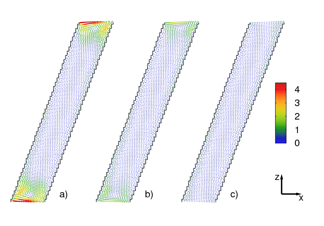
Figure 2: Velocity difference fields for different approaches: In- and outflow velocity constraint to the direction perpendicular to the boundary plane (a), In- and outflow velocity tilted and of parabolic shape as in the analytic solution, but with $N^{z}_{x}$ and $N^{z}_{y}$ set equal to zero (b), the boundary conditions derived in Sec. IV with the correct choice for $N^{z}_{x}$ and $N^{z}_{y}$. difference field (c). The velocity difference vectors are scaled for drawing by a factor of 1500 and the absolute value of the velocity difference is color coded from blue (small) to red (large).

In Fig. 2 a) we apply the boundary condition used by Kutay et al.  Kutay et al. (2006) to a case, where the restriction of the in- and outflow velocity parallel to the $z$-direction introduces an error in the region close to the boundary. Note that in LABEL:Kutay06, apart from assuming the velocity perpendicular to the boundary, the authors underestimate the transversal components, which may be of no importance in this case. We use the correct coefficients as presented very recently in LABEL:Mattila09, but keep the restriction to the inflow perpendicular to the boundary, which has a much larger influence on the flow field. Not only the first and second layer of nodes close to the boundary are affected, but the boundary condition introduces vortices which have approximately the size of the diameter of the channel. Therefore, the first step to generalize the boundary condition from LABEL:Kutay06 to a case where the in- and outflow velocity has an arbitrary orientation, is to use Eqns. (17)–(20), as used in the simulation for which the result is shown in Fig. 2 b). It is obvious that this boundary condition still introduces vortices close to the in- and outflow. The strength of the vortices is smaller compared to the case shown in Fig. 2 a). However, the size of the vortices is comparable to the width of the channel here as well. The value of the tangential velocity on the boundary nodes differs from the value one inserts into the equations. By introducing the transversal momentum corrections $N^{z}_{x}$ and $N^{z}_{y}$ in Eqns. (21)–(24), the vortices disappear and the velocity takes exactly the value one specifies with Eqns. (9)–(11) as one can see in Fig. 2 c). The remaining differencefield can be mostly ascribed to the discretization on the lattice. Each single step of the wall discretized to individual steps can be found in the flow profile. However, at the in- and outflux boundary no additional artifacts can be seen, which demonstrates the strength of our boundary condition. The velocity on the boundary nodes takes exactly the value which we specify, and therefore, no vortices are generated.

The transversal momentum corrections $N^{z}_{x}$ and $N^{z}_{y}$ could also be understood in terms of a counter-slip similar to the approach of Inamuro et al.  Inamuro et al. (1995), but the Ansatz how to obtain the unknown populations $f_{i}$ is different: we assume a bounce back rule for the non-equilibrium part of the distributions and end up with a linear correction to the reflected populations, whereas the authors of LABEL:inamuro95 construct the unknown distributions based on kinetic theory where the correction appears not on the level of the distribution functions but as a counter-slip on the level of the wall velocity. The values for the density and the velocity inserted into the equilibrium distributions in Inamuro’s method are different from the ones used for bulk nodes. In our approach, however, the boundary nodes are treated similar as the bulk nodes: the velocity on the boundary node can be calculated by inserting Eq. (25) and Eq. (26) into Eqns. (21)–(24) and the obtained distributions $f_{i}$ together with the one from Eq. (16) and the density from Eq. (IV) into Eq. (5). It turns out that the velocity calculated from Eq. (5) is exactly the one which is imposed at the boundary node by Eqns. (21)–(24).

In all simulations we kept the tilting angle of the channel constant, because the error of our boundary conditon is angle independent. We can quantify the quality of the boundary conditions by computing the ratio of the absolute value of the difference field and the calculated velocity field on each node. The obtained values are averaged over the first twenty layers of LB nodes from the boundary.

$$\xi=\int\limits_{V}\frac{\left|\mathbf{v}(\mathbf{x})-\mathbf{v}^{P}(\mathbf{x})\right|}{\left|\mathbf{v}^{P}(\mathbf{x})\right|}\mathrm{d}V\,,$$ (35)

Where the volume $V$ contains those layers of lattice nodes, which are at most a distance of the channel width apart from the boundary of the computational domain. This captures approximately the vortices and provides a measure for the quality of the boundary condition. The results for the different cases shown in Fig. 2 are listed in the following tabular:

Boundary condition	relative error $\xi$
on-site velocity (Fig. 2 c)	0.0996
$N^{z}_{x}$ and $N^{z}_{y}$ set to zero (Fig. 2 b)	0.126
$v_{x}=v_{y}=0$ (Fig. 2 a)	0.175

Good agreement with the expected Poiseuille flow profile (Eq. (34)) is reflected in small relative errors. Large numbers indicate deviations in the area, where the fluid fields are compared. We ascribe the remaining deviations to the discretization error of the wall and the accompanying uncertainty in the exact wall position in the present case of the staircase like discretization. We check this by increasing the resolution of the simulation by a factor of two. As we expect, the numerical error due to the staircase-like discretization decreases roughly by a factor of two to $\xi=0.051$. This shows that the staircase-like discretization introduces a first order error. Therefore, we need further investigations to see the second order accuracy of the in- and outflux boundary condition.

As another test for the flux boundary condtion we simulate a straight channel aligned parallel to the computational lattice, again in a $64\times 8\times 128$-domain with the same boundary conditions as for the inclined channel. The remaining relative error decreases to $0.00235$, which is typical for Poiseuille flow simulations at this resolution in combination with a mid-grid bounce back rule on the boundary.

We can further measure the quality of our boundary condition in a shear simulation. On a $32^{3}$ lattice we apply periodic boundaries in $x$- and $y$-direction and impose a shear velocity of $v_{x}=\pm 0.02$ with opposite sign on the top and bottom plane. We obtain a linear flow profile within floating point precision. There are no notable jumps between the first and second layer of LB nodes, which confirms that the strain rate tensor ${\bf\Pi}$ is set up correctly on the boundary nodes.

Figure 3: Poiseuille flow between two parallel walls driven by a body force. The simulation data are averaged in each lattice plane parallel to the walls and agree up to floating point precision with the calculated Poiseuille profile.

In a next step we simulate Poiseuille flow again, but this time we use a $32^{3}$ lattice with periodic boundaries in $y$- and $z$- direction. We apply a body force Harting et al. (2005); Guo et al. (2002) by adding a force term

$$\Delta\mathbf{v}=\frac{\tau\mathbf{F}}{\rho}$$ (36)

to the velocity in Eq. (6) in the whole simulation volume. The Poiseuille profile we expect is of the form

$$\mathbf{v}=\frac{\mathbf{F}}{2\eta}\left(1-\left(\frac{x-x_{0}}{\Delta x}\right)^{2}\right)\,,$$ (37)

where the viscosity is given by Eq. (8). The velocity profile found in the simulation together with the expected Poiseuille profile is plotted in Fig. 3. The parabola contains no fit parameters. The velocity is exactly zero on the boundary nodes, whereas with a simple bounce-back a numerical slip can be observed, which results in a velocity of $4\times 10^{-5}$ for the same simulation setup without using the transversal momentum corrections $N^{z}_{x}$ and $N^{z}_{y}$. We have carried out this test with $\tau=1$, but the data presented in Fig. 3 is obtained with $\tau=2$ to ensure that our boundary conditions are not restricted to the special case of $\tau=1$. Apart from the influence of $\tau$ on the viscosity (Eq. (8)), our simulation results are not affected by the relaxation time. In particular, we do not see any $\tau$-dependent (numerical) slip.

a)
b)
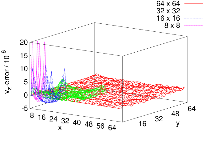
c)

Figure 4: a) Velocity profile in a square channel averaged along the $yz$-planes for the noslip boundary condition (squares), for the node based bounce back rule (triangles), mid-link bounce back (top down triangles), and the analytical solution. The noslip boundary condition collapses with the analytical solution, whereas the on-site bounce back boundary condition shows a kink in the profile close to the boundary nodes. The numerical results are obtained on a $32^{3}$ lattice and for the analytical solution the sum in Eq. (38) is truncated after 50 terms. A 2D profile of the $z$-velocity in a $xy$-cross section is displayed as an inset.
b) The relative error for system sizes between 8 and 64 nodes: in the corners next to the boundary the largest relative deviations occur. Note that on the boundary nodes, where the truncation error of Eq. (38) is largest, the deviation between simulation and approximated analytical solution is negligible. Therefore, the deviation can be taken as a measure for the quality of the numerical result.
c) The averaged error for different lattice resolutions versus the number of lattice nodes in each dimension confirming the second order accuracy of the no-slip boundary condition.

Also in this second-order test we find that the numerical error is of the size of the floating point precision on the computer. This underlines that our boundary condition reproduces the velocity field up to second order.

Finally, we test our implementation by simulating flow through a square channel. The analytical solution for the velocity of a pressure driven flow in a $b\times b$ square channel is Wieghardt (1957)

$$\mathbf{v}(x,y) = -\frac{\nabla p}{2\eta}\left[\frac{b^{2}}{4}-y^{2}-C(x)\right],\mathrm{with}$$ (38)

$$C(x) = \frac{8b^{2}}{\pi^{3}}\sum\limits_{n=0}^{\infty}(-1)^{n}\frac{\cosh\left(\frac{(2n+1)\pi x}{b}\right)\cos\left(\frac{(2n+1)\pi y}{b}\right)}{(2n+1)^{3}\cosh\left(\frac{(2n+1)\pi}{2}\right)}$$

where $x\in[-b/2,b/2]$ and $y\in[-b/2,b/2]$ are the coordinates in the cross-section, with the origin in the center of the channel. The pressure gradient $\nabla p$ is imposed by pressure boundaries and the dynamic viscosity is known from Eq. (8). The infinite sum in Eq. (38) can be truncated when a given accuracy is reached. We sum up 50 terms and compare this approximation to our numerical results on a $32^{3}$ domain, i.e., $b=15$ plus one layer of boundary nodes. In Fig. 4 a) we compare the analytical solution from Eq. (38) with our simulation results. The velocity in $z$-direction is averaged over the $y$- and $z$-direction and the averaged value is plotted against the position in $x$-direction. A very good agreement of the numerical result with the analytical solution can be seen. For comparison, results for the node based bounce back rule are shown. For this boundary condition it is known that it is only first oderer accurate, which can be seen in the kink in the velocity profile close to the boundary nodes. It can however be made second order accurate by choosing the position of the wall somewhere (depending on the BGK relaxation time) in between two nodes, which is known as the mid-grid bounce back Succi (2001). As one can see in Fig. 4 a), if the wall-position is chosen correctly for the bounce-back rule, a satisfiying accuracy can be achieved, too (top-down triangles). Note that the position of the wall is shifted by half a lattice unit due to the different approach at the wall.

In Fig. 4 b) the relative error depending on the size of the simulation is studied. There are three different errors involved. The truncation errors of the sum in Eq. (38) can not be seen in this figure. If the sum is truncated after just a few terms, the error increases on two of the edges. In the corners of the simulation domain the errors due to the discretization on the lattice remains. This is what determines the accuracy for relatively small simulations. However, if the lattice is refined, this error decreases. It decreases with the square of the lattice constant which is typical for second order accurate schemes. Another error which dominates for large systems is the floating point precision which is reflected in noisy data in the center of the simulation domain. This error is independent on the lattice constant. In Fig. 4 b) the relative error is shown for different system sizes. In the corners the error decreases with the system size, whereas the noise in the center is independent by the system size. In Fig. 4 c) we plot the mean error averaged over the whole system against the number of lattice nodes used for computation in each dimension. The slope of approximately $2$ confirms the second order accuracy of the boundary condition. For the simulations presented in Fig. 4 pressure boundaries according to Eq. (IV) are used and on the walls and edges we apply no-slip conditions as described in Sec. V. For this plot we use only the range in which the lattice size dependent error dominates. For 64 lattice nodes in each dimension, the floating point precision in one of our post processing steps dominates the overall error. Therefore, we only use the smaller systems for this investigation. The inset in Fig. 4 shows the analytical velocity profile in a cross section perpendicular to the extension of the square channel.

VII Conclusion

We have derived an explicit local on-site flux boundary condition for LB simulations on a D3Q19 lattice. Velocity terms up to second order enter the derivation and this accuracy is also confirmed in the numerical tests. The in- and outflux velocity underlies no restrictions to any peculiar direction. We have demonstrated the numerical accuracy by comparing simulation results for a flow through a tilted channel with the theoretical expectation of a Poiseuille flow. Remaining errors can be assigned to the discretization on the lattice and to rounding errors due to the floating point representation. We have tested the boundary condition in simulation of Poiseuille flow between two planar walls and in shear flow. In those tests the simulation data fits exactly the analytical solutions without any slip-parameter and independent on the BGK relaxation time. For this test we have used no-slip boundary conditions which are a special case included in the general velocity boundary conditions. Finally, we have tested the boundary condition by simulating the flow through a square channel. The scaling of the numerical error with the lattice resolution again confirms the second order accuracy.

Appendix

Here we give the expressions for the other boundaries not treated explicitly in the text. We start with the top-plane where we implement outflux for our simulations. We obtain

$$\rho = \frac{1}{v_{z}+1}\left[f_{1}+f_{2}+f_{3}+f_{4}\right.$$

$$+f_{7}+f_{11}+f_{12}+f_{8}+f_{19}+$$

$$\left.2(f_{5}+f_{9}+f_{13}+f_{15}+f_{17})\right]$$

or

$$v_{z} = -1+\frac{1}{\rho_{0}}\left[f_{1}+f_{2}+f_{3}+f_{4}\right.$$

$$+f_{7}+f_{11}+f_{12}+f_{8}+f_{19}+$$

$$\left.2(f_{5}+f_{9}+f_{13}+f_{15}+f_{17})\right]$$

with $v_{z}$ defined in positive $z$-direction. Here, the undetermined populations after the streaming step are

$$f_{6} = f_{5}-\frac{1}{3}\rho v_{z}\,,$$ (41)

$$f_{10} = f_{13}+\frac{\rho}{6}(-v_{z}+v_{x})-N^{z}_{x}\,,$$ (42)

$$f_{14} = f_{9}+\frac{\rho}{6}(-v_{z}-v_{x})+N^{z}_{x}\,,$$ (43)

$$f_{16} = f_{17}+\frac{\rho}{6}(-v_{z}+v_{y})-N^{z}_{y}\,,$$ (44)

$$f_{18} = f_{15}+\frac{\rho}{6}(-v_{z}-v_{y})+N^{z}_{y}$$ (45)

with $N^{z}_{x}$ and $N^{z}_{y}$ defined as previously, in Eq. (25) and Eq. (26).

For the left, right, front and back boundaries, which we do not use in this work one finds the following expressions. For the left ($x=0$) boundary as inlet,

$$\rho = \frac{1}{1-v_{x}}\left[f_{3}+f_{4}+f_{5}+f_{6}\right.$$

$$+ f_{15}+f_{16}+f_{17}+f_{18}+f_{19}$$

$$+ \left.2(f_{2}+f_{11}+f_{12}+f_{13}+f_{14})\right]\,,$$

or

$$v_{x} = 1-\frac{1}{\rho_{0}}\left[f_{3}+f_{4}+f_{5}+f_{6}\right.$$

$$+ f_{15}+f_{16}+f_{17}+f_{18}+f_{19}$$

$$+ \left.2(f_{2}+f_{11}+f_{12}+f_{13}+f_{14})\right]\,,$$

and

$$f_{1} = f_{2}+\frac{1}{3}\rho v_{x}\,,$$ (48)

$$f_{8} = f_{11}+\frac{\rho}{6}(v_{x}-v_{y})+N^{x}_{y}\,,$$ (49)

$$f_{7} = f_{12}+\frac{\rho}{6}(v_{x}+v_{y})-N^{x}_{y}\,,$$ (50)

$$f_{9} = f_{14}+\frac{\rho}{6}(v_{x}+v_{z})-N^{x}_{z}\,,$$ (51)

$$f_{10} = f_{13}+\frac{\rho}{6}(v_{x}-v_{z})+N^{x}_{z}$$ (52)

with

$$N^{x}_{y} = \frac{1}{2}\left[f_{3}+f_{15}+f_{16}-(f_{4}+f_{17}+f_{18})\right]$$ (53)

$$-\frac{1}{3}\rho v_{y}\,,$$

$$N^{x}_{z} = \frac{1}{2}\left[f_{5}+f_{17}+f_{15}-(f_{6}+f_{16}+f_{18})\right]$$ (54)

$$-\frac{1}{3}\rho v_{z}\,.$$

At the right boundary (outlet) we have

$$\rho = \frac{1}{v_{x}+1}\left[f_{3}+f_{4}+f_{5}+f_{6}\right.$$

$$+ f_{15}+f_{16}+f_{17}+f_{18}+f_{19}$$

$$+ \left.2(f_{1}+f_{7}+f_{8}+f_{9}+f_{10})\right]\,,$$

or

$$v_{x}=-1 + \frac{1}{\rho_{0}}\left[f_{3}+f_{4}+f_{5}+f_{6}\right.$$

$$+ f_{15}+f_{16}+f_{17}+f_{18}+f_{19}$$

$$+ \left.2(f_{1}+f_{7}+f_{8}+f_{9}+f_{10})\right]\,,$$

and

$$f_{2} = f_{1}-\frac{1}{3}\rho v_{x}\,,$$ (57)

$$f_{11} = f_{8}+\frac{\rho}{6}(-v_{x}+v_{y})-N^{x}_{y}\,,$$ (58)

$$f_{12} = f_{7}+\frac{\rho}{6}(-v_{x}-v_{y})+N^{x}_{y}\,,$$ (59)

$$f_{14} = f_{9}+\frac{\rho}{6}(-v_{x}-v_{z})+N^{x}_{z}\,,$$ (60)

$$f_{13} = f_{10}+\frac{\rho}{6}(-v_{x}+v_{z})-N^{x}_{z}\,.$$ (61)

At the front ($y=0$) boundary as inlet, one finds

$$\rho = \frac{1}{1-v_{y}}\left[f_{1}+f_{2}+f_{5}+f_{6}\right.$$

$$+ f_{9}+f_{10}+f_{13}+f_{14}+f_{19}$$

$$+ \left.2(f_{4}+f_{8}+f_{12}+f_{17}+f_{18})\right]\,,$$

or

$$v_{y}=1 - \frac{1}{\rho_{0}}\left[f_{1}+f_{2}+f_{5}+f_{6}\right.$$

$$+ f_{9}+f_{10}+f_{13}+f_{14}+f_{19}$$

$$+ \left.2(f_{4}+f_{8}+f_{12}+f_{17}+f_{18})\right]\,,$$

and

$$f_{3} = f_{4}+\frac{1}{3}\rho v_{y}\,,$$ (64)

$$f_{7} = f_{12}+\frac{\rho}{6}(v_{y}+v_{x})-N^{y}_{x}\,,$$ (65)

$$f_{11} = f_{8}+\frac{\rho}{6}(v_{y}-v_{x})+N^{y}_{x}\,,$$ (66)

$$f_{15} = f_{18}+\frac{\rho}{6}(v_{y}+v_{z})-N^{y}_{z}\,,$$ (67)

$$f_{16} = f_{17}+\frac{\rho}{6}(v_{y}-v_{z})+N^{y}_{z}$$ (68)

with

$$N^{y}_{x} = \frac{1}{2}\left[f_{1}+f_{9}+f_{10}-(f_{2}+f_{13}+f_{14})\right]$$ (69)

$$-\frac{1}{3}\rho v_{x}\,,$$

$$N^{y}_{z} = \frac{1}{2}\left[f_{5}+f_{9}+f_{13}-(f_{6}+f_{10}+f_{14})\right]$$ (70)

$$-\frac{1}{3}\rho v_{z}\,.$$

At the back (outlet) the density is given by

$$\rho = \frac{1}{v_{y}+1}\left[f_{1}+f_{2}+f_{5}+f_{6}\right.$$

$$+ f_{9}+f_{10}+f_{13}+f_{14}+f_{19}$$

$$+ \left.2(f_{3}+f_{7}+f_{11}+f_{15}+f_{16})\right]\,,$$

or the velocity reads

$$v_{x} = -1+\frac{1}{\rho_{0}}\left[f_{1}+f_{2}+f_{5}+f_{6}\right.$$

$$+ f_{9}+f_{10}+f_{13}+f_{14}+f_{19}$$

$$+ \left.2(f_{3}+f_{7}+f_{11}+f_{15}+f_{16})\right]\,,$$

and the distributions are

$$f_{4} = f_{3}-\frac{1}{3}\rho v_{y}\,,$$ (73)

$$f_{12} = f_{7}+\frac{\rho}{6}(-v_{y}-v_{x})+N^{y}_{x}\,,$$ (74)

$$f_{8} = f_{11}+\frac{\rho}{6}(-v_{y}+v_{x})-N^{y}_{x}\,,$$ (75)

$$f_{18} = f_{15}+\frac{\rho}{6}(-v_{y}-v_{z})+N^{y}_{z}\,,$$ (76)

$$f_{17} = f_{16}+\frac{\rho}{6}(-v_{y}+v_{z})-N^{y}_{z}\,.$$ (77)

References

- Zou and He (1997) Q. Zou and X. He, Phys. Fluids 9, 1591 (1997).
- Succi (2001) S. Succi, The lattice Boltzmann equation for fluid dynamics and beyond (Oxford University Press, 2001).
- Chen et al. (1992) H. Chen, S. Chen, and W. H. Matthaeus, Phys. Rev. A 45, R5339 (1992).
- Higuera et al. (1989) F. J. Higuera, S. Succi, and R. Benzi, Europhys. Lett. 9, 345 (1989).
- Kutay et al. (2006) M. E. Kutay, A. H. Aydilek, and E. Masad, Comp. Geotech. 33, 381 (2006).
- Martys and Chen (1996) N. S. Martys and H. Chen, Phys. Rev. E 53, 743 (1996).
- Ladd (1994a) A. J. C. Ladd, J. Fluid Mech. 271, 285 (1994a).
- Ladd (1994b) A. J. C. Ladd, J. Fluid Mech. 271, 311 (1994b).
- Ladd and Verberg (2001) A. J. C. Ladd and R. Verberg, J. Stat. Phys. 104, 1191 (2001).
- Harting et al. (2008) J. Harting, H. Herrmann, and E. Ben-Naim, Europhys. Lett. 83, 30001 (2008).
- Shan and Chen (1993) X. Shan and H. Chen, Phys. Rev. E 47, 1815 (1993).
- Shan and Chen (1994) X. Shan and H. Chen, Phys. Rev. E 49, 2941 (1994).
- Chen et al. (2000) H. Chen, B. M. Boghosian, P. V. Coveney, and M. Nekovee, Proc. R. Soc. Lond. A 456, 2043 (2000).
- Harting et al. (2005) J. Harting, J. Chin, M. Venturoli, and P. V. Coveney, Phil. Trans. R. Soc. Lond. A 363, 1895 (2005).
- Chin and Coveney (2002) J. Chin and P. V. Coveney, Phys. Rev. E 66, 016303 (2002).
- Frisch et al. (1987) U. Frisch, D. d’Humières, B. Hasslacher, P. Lallemand, Y. Pomeau, and J. P. Rivet, Complex Systems 1, 649 (1987).
- Ginzburg and Steiner (2003) I. Ginzburg and K. Steiner, J. Comp. Phys. 185, 61 (2003).
- Skordos (1993) P. A. Skordos, Phys. Rev. E 48, 4823 (1993).
- Ginzbourg and d’Humières (1996) I. Ginzbourg and D. d’Humières, J. Stat. Phys. 84, 927 (1996).
- Mattila et al. (2009) K. Mattila, J. Hyväluoma, and T. Rossi, J. Stat. Mech. 6, P06015 (2009).
- Qian (1997) Y. Qian, Int. J. Mod. Phys. C 8, 753 (1997).
- Zou et al. (1995) Q. Zou, S. Hou, S. Chen, and G. D. Doolen, J. Stat. Phys. 81, 35 (1995).
- Karniadakis et al. (2005) G. Karniadakis, A. Beskok, and N. Aluru, Microflows and nanoflows, fundamentals and simulation (Springer, 2005).
- Hessel et al. (2005) V. Hessel, H. Löwe, and F. Schönfeld, Chem. Eng. Sci 60, 2479 (2005).
- Inamuro et al. (1995) T. Inamuro, M. Yoshino, and F. Ogino, Phys. Fluids 7, 2928 (1995).
- Maier et al. (1996) R. S. Maier, R. S. Bernard, and D. W. Grunau, Phys. Fluids 8, 1788 (1996).
- Flekkøy et al. (2000) E. G. Flekkøy, G. Wagner, and J. Feder, Europhys. Lett. 52, 271 (2000).
- Delgado-Buscalioni and Coveney (2003) R. Delgado-Buscalioni and P. V. Coveney, Phys. Rev. E 67, 046704 (2003).
- Delgado-Buscalioni et al. (2008) R. Delgado-Buscalioni, K. Kremer, and M. Praprotnik, J. Chem. Phys. 128, 114110 (2008).
- Dupuis et al. (2007) A. Dupuis, E. M. Kotsalis, and P. Koumoutsakos, Phys. Rev. E 75, 046704 (2007).
- Bhatnagar et al. (1954) P. L. Bhatnagar, E. P. Gross, and M. Krook, Phys. Rev. 94, 511 (1954).
- McNamara and Zanetti (1988) G. R. McNamara and G. Zanetti, Phys. Rev. Lett. 61, 2332 (1988).
- He and Luo (1997) X. He and L. S. Luo, Phys. Rev. E 56, 6811 (1997).
- Note (1) Note that some authors, e.g. in Ref.\tmspace+.1667emKutay et al. (2006), use a different notation in which the vectors are permutated, and as well as and are exchanged. Sometimes is denoted as .
- Qian et al. (1992) Y. H. Qian, D. d’Humières, and P. Lallemand, Europhys. Lett. 17, 479 (1992).
- Tang et al. (2005) G. H. Tang, W. Q. Tao, and Y. L. He, Phys. Rev. E 72, 016703 (2005).
- Sbragaglia and Succi (2005) M. Sbragaglia and S. Succi, Phys. Fluids 17, 093602 (2005).
- Chen et al. (1996) S. Chen, D. Martínez, and R. Mei, Phys. Fluids 8, 2527 (1996).
- Hänel (2004) D. Hänel, Molekulare Gasdynamik : Einführung in die kinetische Theorie der Gase und Lattice-Boltzmann-Methoden (Springer, Berlin, 2004).
- Sukop and Thorne (2007) M. C. Sukop and D. T. Thorne, Lattice Boltzmann Modeling (Springer Berlin Heidelberg New York, 2007).
- Ansumali and Karlin (2002) S. Ansumali and I. V. Karlin, Phys. Rev. E 66, 026311 (2002).
- d’Orazio et al. (2003) A. d’Orazio, S. Succi, and C. Arrighetti, Phys. Fluids 15, 2778 (2003).
- Verberg and Ladd (2001) R. Verberg and A. J. C. Ladd, Phys. Rev. E 65, 016701 (2001).
- Chun and Ladd (2007) B. Chun and A. J. C. Ladd, Phys. Rev. E 75, 066705 (2007).
- Schiller (2008) U. D. Schiller, Thermal fluctuations and boundary conditions in the lattice Boltzmann method, Ph.D. thesis, Johannes Gutenberg-Universität Mainz, Germany (2008).
- Latt et al. (2008) J. Latt, B. Chopard, O. Malaspinas, M. Deville, and A. Michler, Phys. Rev. E 77, 056703 (2008).
- Halliday et al. (2002) I. Halliday, L. A. Hammond, and C. M. Care, J. Phys. A. 35, L157 (2002).
- Note (2) Values of 19 onwards as vector index can be used to distinguish the different corner nodes.
- Guo et al. (2002) Z. Guo, C. Zheng, and B. Shi, Phys. Rev. E 65, 046308 (2002).
- Wieghardt (1957) K. Wieghardt, Theoretische Strömungslehre (Göttinger Klassik, 1957).