Dynamics of postcritically bounded polynomial semigroups III: classification of semi-hyperbolic semigroups and random Julia sets which are Jordan curves but not quasicircles

Abstract

We investigate the dynamics of polynomial semigroups (semigroups generated by a family of polynomial maps on the Riemann sphere $\hat{\mathbb{C}}$) and the random dynamics of polynomials on the Riemann sphere. Combining the dynamics of semigroups and the fiberwise (random) dynamics, we give a classification of polynomial semigroups $G$ such that $G$ is generated by a compact family $\Gamma$, the planar postcritical set of $G$ is bounded, and $G$ is (semi-) hyperbolic. In one of the classes, we have that for almost every sequence $\gamma\in\Gamma^{\mathbb{N}}$, the Julia set $J_{\gamma}$ of $\gamma$ is a Jordan curve but not a quasicircle, the unbounded component of $\hat{\mathbb{C}}\setminus J_{\gamma}$ is a John domain, and the bounded component of $\mathbb{C}\setminus J_{\gamma}$ is not a John domain. Note that this phenomenon does not hold in the usual iteration of a single polynomial. Moreover, we consider the dynamics of polynomial semigroups $G$ such that the planar postcritical set of $G$ is bounded and the Julia set is disconnected. Those phenomena of polynomial semigroups and random dynamics of polynomials that do not occur in the usual dynamics of polynomials are systematically investigated.

1 Introduction

This is the third paper in which the dynamics of semigroups of polynomial maps with bounded planar postcritical set in $\mathbb{C}$ are investigated. This paper is self-contained and the proofs of the results of this paper are independent from the results in [37, 38].

The theory of complex dynamical systems, which has its origin in the important work of Fatou and Julia in the 1910s, has been investigated by many people and discussed in depth. In particular, since D. Sullivan showed the famous “no wandering domain theorem” using Teichmüller theory in the 1980s, this subject has attracted many researchers from a wide area. For a general reference on complex dynamical systems, see Milnor’s textbook [16].

There are several areas in which we deal with generalized notions of classical iteration theory of rational functions. One of them is the theory of dynamics of rational semigroups (semigroups generated by a family of holomorphic maps on the Riemann sphere $\hat{\mathbb{C}}$), and another one is the theory of random dynamics of holomorphic maps on the Riemann sphere.

In this paper, we will discuss these subjects. A rational semigroup is a semigroup generated by a family of non-constant rational maps on $\hat{\mathbb{C}}$, where $\hat{\mathbb{C}}$ denotes the Riemann sphere, with the semigroup operation being functional composition ([12]). A polynomial semigroup is a semigroup generated by a family of non-constant polynomial maps. Research on the dynamics of rational semigroups was initiated by A. Hinkkanen and G. J. Martin ([12, 13]), who were interested in the role of the dynamics of polynomial semigroups while studying various one-complex-dimensional moduli spaces for discrete groups, and by F. Ren’s group([45, 11]), who studied such semigroups from the perspective of random dynamical systems. Moreover, the research on rational semigroups is related to that on “iterated function systems” in fractal geometry. In fact, the Julia set of a rational semigroup generated by a compact family has “ backward self-similarity” (cf. Lemma 3.1-2). For other research on rational semigroups, see [20, 21, 22, 44, 23, 24, 42, 41, 43], and [27]–[39].

The research on the dynamics of rational semigroups is also directly related to that on the random dynamics of holomorphic maps. The first study in this direction was by Fornaess and Sibony ([9]), and much research has followed. (See [1, 3, 4, 2, 10, 34, 39].)

We remark that the complex dynamical systems can be used to describe some mathematical models. For example, the behavior of the population of a certain species can be described as the dynamical system of a polynomial $f(z)=az(1-z)$ such that $f$ preserves the unit interval and the postcritical set in the plane is bounded (cf. [8]). It should also be remarked that according to the change of the natural environment, some species have several strategies to survive in the nature. From this point of view, it is very important to consider the random dynamics of such polynomials (see also Example 1.4). For the random dynamics of polynomials on the unit interval, see [26].

We shall give some definitions for the dynamics of rational semigroups.

Definition 1.1 ([12, 11]).

Let $G$ be a rational semigroup. We set

$$F(G)=\{z\in\hat{\mathbb{C}}\mid G\mbox{ is normal in a neighborhood of $z$}\},\mbox{ and }\ J(G)=\hat{\mathbb{C}}\setminus F(G).$$

$F(G)$ is called the Fatou set of $G$ and $J(G)$ is called the Julia set of $G$. We let $\langle h_{1},h_{2},\ldots\rangle$ denote the rational semigroup generated by the family $\{h_{i}\}.$ More generally, for a family $\Gamma$ of non-constant rational maps, we denote by $\langle\Gamma\rangle$ the rational semigroup generated by $\Gamma.$ The Julia set of the semigroup generated by a single map $g$ is denoted by $J(g).$ Similarly, we set $F(g):=F(\langle g\rangle).$

Definition 1.2.

1. For each rational map $g:\hat{\mathbb{C}}\rightarrow\hat{\mathbb{C}}$, we set $CV(g):=\{\mbox{all critical values of }g:\hat{\mathbb{C}}\rightarrow\hat{\mathbb{C}}\}.$ Moreover, for each polynomial map $g:\hat{\mathbb{C}}\rightarrow\hat{\mathbb{C}}$, we set $CV^{\ast}(g):=CV(g)\setminus\{\infty\}.$

2. Let $G$ be a rational semigroup. We set

   $$P(G):=\overline{\bigcup_{g\in G}CV(g)}\ (\subset\hat{\mathbb{C}}).$$

   This is called the postcritical set of $G.$ Furthermore, for a polynomial semigroup $G$, we set $P^{\ast}(G):=P(G)\setminus\{\infty\}.$ This is called the planar postcritical set (or finite postcritical set) of $G.$ We say that a polynomial semigroup $G$ is postcritically bounded if $P^{\ast}(G)$ is bounded in $\mathbb{C}.$

Remark 1.3.

Let $G$ be a rational semigroup generated by a family $\Lambda$ of rational maps. Then, we have that $P(G)=\overline{\bigcup_{g\in G\cup\{Id\}}\ g(\bigcup_{h\in\Lambda}CV(h))}$, where Id denotes the identity map on $\hat{\mathbb{C}}.$ Thus $g(P(G))\subset P(G)$ for each $g\in G.$ From this formula, one can figure out how the set $P(G)$ (resp. $P^{\ast}(G)$) spreads in $\hat{\mathbb{C}}$ (resp. $\mathbb{C}$). In fact, in Section 5, using the above formula, we present a way to construct examples of postcritically bounded polynomial semigroups (with some additional properties). Moreover, from the above formula, one may, in the finitely generated case, use a computer to see if a polynomial semigroup $G$ is postcritically bounded much in the same way as one verifies the boundedness of the critical orbit for the maps $f_{c}(z)=z^{2}+c.$

Example 1.4.

Let $\Lambda:=\{h(z)=cz^{a}(1-z)^{b}\mid a,b\in\mathbb{N},\ c>0,\ c(\frac{a}{a+b})^{a}(\frac{b}{a+b})^{b}$ $\leq 1\}$ and let $G$ be the polynomial semigroup generated by $\Lambda.$ Since for each $h\in\Lambda$, $h([0,1])\subset[0,1]$ and $CV^{\ast}(h)\subset[0,1]$, it follows that each subsemigroup $H$ of $G$ is postcritically bounded.

Remark 1.5.

It is well-known that for a polynomial $g$ with $\deg(g)\geq 2$, $P^{\ast}(\langle g\rangle)$ is bounded in $\mathbb{C}$ if and only if $J(g)$ is connected ([16, Theorem 9.5]).

As mentioned in Remark 1.5, the planar postcritical set is one piece of important information regarding the dynamics of polynomials. Concerning the theory of iteration of quadratic polynomials, we have been investigating the famous “Mandelbrot set”.

When investigating the dynamics of polynomial semigroups, it is natural for us to discuss the relationship between the planar postcritical set and the figure of the Julia set. The first question in this regard is:

Question 1.6.

Let $G$ be a polynomial semigroup such that each element $g\in G$ is of degree two or more. Is $J(G)$ necessarily connected when $P^{\ast}(G)$ is bounded in $\mathbb{C}$?

The answer is NO.

Example 1.7 ([44]).

Let $G=\langle z^{3},\frac{z^{2}}{4}\rangle.$ Then $P^{\ast}(G)=\{0\}$ (which is bounded in $\mathbb{C}$) and $J(G)$ is disconnected ($J(G)$ is a Cantor set of round circles). Furthermore, according to [32, Theorem 2.4.1], it can be shown that a small perturbation $H$ of $G$ still satisfies that $P^{\ast}(H)$ is bounded in $\mathbb{C}$ and that $J(H)$ is disconnected. ($J(H)$ is a Cantor set of quasi-circles with uniform dilatation.)

Question 1.8.

What happens if $P^{\ast}(G)$ is bounded in $\mathbb{C}$ and $J(G)$ is disconnected?

Problem 1.9.

Classify postcritically bounded polynomial semigroups.

Definition 1.10.

Let ${\cal G}$ be the set of all polynomial semigroups $G$ with the following properties:

• each element of $G$ is of degree two or more, and

• $P^{\ast}(G)$ is bounded in $\mathbb{C}$, i.e., $G$ is postcritically bounded.

Furthermore, we set ${\cal G}_{con}=\{G\in{\cal G}\mid J(G)\mbox{ is connected}\}$ and ${\cal G}_{dis}=\{G\in{\cal G}\mid J(G)\mbox{ is disconnected}\}.$

We also investigate the dynamics of hyperbolic or semi-hyperbolic polynomial semigroups.

Definition 1.11.

Let $G$ be a rational semigroup.

1. We say that $G$ is hyperbolic if $P(G)\subset F(G).$

2. We say that $G$ is semi-hyperbolic if there exists a number $\delta>0$ and a number $N\in\mathbb{N}$ such that, for each $y\in J(G)$ and each $g\in G$, we have $\deg(g:V\rightarrow B(y,\delta))\leq N$ for each connected component $V$ of $g^{-1}(B(y,\delta))$, where $B(y,\delta)$ denotes the ball of radius $\delta$ with center $y$ with respect to the spherical distance, and $\deg(g:\cdot\rightarrow\cdot)$ denotes the degree of finite branched covering. (For the background of semi-hyperbolicity, see [27] and [30].)

Remark 1.12.

There are many nice properties of hyperbolic or semi-hyperbolic rational semigroups. For example, for a finitely generated semi-hyperbolic rational semigroup $G$ , there exists an attractor in the Fatou set ([27, 30]), and the Hausdorff dimension $\dim_{H}(J(G))$ of the Julia set is less than or equal to the critical exponent $s(G)$ of the Poincaré series of $G$ ([27]). If we assume further the “open set condition”, then $\dim_{H}(J(G))=s(G)$ ([33, 43]). Moreover, if $G\in{\cal G}$ is generated by a compact set $\Gamma$ and if $G$ is semi-hyperbolic, then for each sequence $\gamma\in\Gamma^{\mathbb{N}}$, the basin of infinity for $\gamma$ is a John domain and the Julia set of $\gamma$ is connected and locally connected ([30]). This fact will be used in the proofs of the main results of this paper.

In this paper, we classify the semi-hyperbolic, postcritically bounded, polynomial semigroups generated by a compact family $\Gamma$ of polynomials. We show that such a semigroup $G$ satisfies either (I) every fiberwise Julia set is a quasicircle with uniform distortion, or (II) for almost every sequence $\gamma\in\Gamma^{\mathbb{N}}$, the Julia set $J_{\gamma}$ is a Jordan curve but not a quasicircle, the basin of infinity $A_{\gamma}$ is a John domain, and the bounded component $U_{\gamma}$ of the Fatou set is not a John domain, or (III) for every $\alpha,\beta\in\Gamma^{\mathbb{N}}$, the intersection of the Julia sets $J_{\alpha}$ and $J_{\beta}$ is not empty, and $J(G)$ is arcwise connected (cf. Theorem 2.19). Furthermore, we also classify the hyperbolic, postcritically bounded, polynomial semigroups generated by a compact family $\Gamma$ of polynomials. We show that such a semigroup $G$ satisfies either (I) above, or (II) above, or (III)’: for every $\alpha,\beta\in\Gamma^{\mathbb{N}}$, the intersection of the Julia sets $J_{\alpha}$ and $J_{\beta}$ is not empty, $J(G)$ is arcwise connected, and for every sequence $\gamma\in\Gamma^{\mathbb{N}}$, there exist infinitely many bounded components of $F_{\gamma}$ (cf. Theorem 2.21). We give some examples of situation (II) above (cf. Example 2.22, figure 1, Example 2.23, and Section 5). Note that situation (II) above is a special phenomenon of random dynamics of polynomials that does not occur in the usual dynamics of polynomials.

The key to investigating the dynamics of postcritically bounded polynomial semigroups is the density of repelling fixed points in the Julia set (cf. Theorem 3.2), which can be shown by an application of the Ahlfors five island theorem, and the lower semi-continuity of $\gamma\mapsto J_{\gamma}$ (Lemma 3.4-2), which is a consequence of potential theory. The key to investigating the dynamics of semi-hyperbolic polynomial semigroups is, the continuity of the map $\gamma\mapsto J_{\gamma}$ (this is highly nontrivial; see [27]) and the Johnness of the basin $A_{\gamma}$ of infinity (cf. [30]). Note that the continuity of the map $\gamma\mapsto J_{\gamma}$ does not hold in general, if we do not assume semi-hyperbolicity. Moreover, one of the original aspects of this paper is the idea of “combining both the theory of rational semigroups and that of random complex dynamics”. It is quite natural to investigate both fields simultaneously. However, no study thus far has done so.

Furthermore, in Section 5, we provide a way of constructing examples of postcritically bounded polynomial semigroups with some additional properties (disconnectedness of Julia set, semi-hyperbolicity, hyperbolicity, etc.) (cf. Lemma 5.1, 5.2, 5.4, 5.5, 5.6). By using this, we will see how easily situation (II) above occurs, and we obtain many examples of situation (II) above.

As wee see in Example 1.4 and Section 5, it is not difficult to construct many examples, it is not difficult to verify the hypothesis “postcritically bounded”, and the class of postcritically bounded polynomial semigroups is very wide.

Throughout the paper, we will see some phenomena in polynomial semigroups or random dynamics of polynomials that do not occur in the usual dynamics of polynomials. Moreover, those phenomena and their mechanisms are systematically investigated.

In Section 2, we present the main results of this paper. We give some tools in Section 3. The proofs of the main results are given in Section 4. In Section 5, we present many examples.

There are many applications of the results of postcritically bounded polynomial semigroups in many directions. In subsequent papers [39, 40], we will investigate Markov process on $\hat{\mathbb{C}}$ associated with the random dynamics of polynomials and we will consider the probability $T_{\infty}(z)$ of tending to $\infty\in\hat{\mathbb{C}}$ starting with the initial value $z\in\hat{\mathbb{C}}.$ It will be shown in [39, 40] that if the associated polynomial semigroup $G$ is postcritically bounded and the Julia set is disconnected, then the function $T_{\infty}$ defined on $\hat{\mathbb{C}}$ has many interesting properties which are similar to those of the Cantor function. For example, under certain conditions, $T_{\infty}$ is continuous on $\hat{\mathbb{C}}$, varies precisely on $J(G)$ which is a thin fractal set, and $T_{\infty}$ has a kind of monotonicity. Such a kind of “singular functions on the complex plane” appear very naturally in random dynamics of polynomials and the study of the dynamics of postcritically polynomial semigroups are the keys to investigating that. (The above results have been announced in [34, 35].)

Moreover, as illustrated before, it is very important for us to recall that the complex dynamics can be applied to describe some mathematical models. For example, the behavior of the population of a certain species can be described as the dynamical systems of a polynomial $h$ such that $h$ preserves the unit interval and the postcritical set in the plane is bounded. When one considers such a model, it is very natural to consider the random dynamics of polynomials with bounded postcritical set in the plane (see Example 1.4).

In [37], we investigate the dynamics of postcritically bounded polynomial semigroups $G$ which is possibly generated by a non-compact family. The structure of the Julia set is deeply studied, and for such a $G$ with disconnected Julia set, it is shown that $J(G)\subset\mathbb{C}$, and that if $A$ and $B$ are two connected components of $J(G)$, then one of them surrounds the other. Therefore the space ${\cal J}_{G}$ of all connected components of $J(G)$ has an intrinsic total order. Moreover, we show that for each $n\in\mathbb{N}\cup\{\aleph_{0}\}$, there exists a finitely generated postcritically bounded polynomial semigroup $G$ such that the cardinality of the space of all connected components of $J(G)$ is equal to $n.$ In [38], by using the results in [37], we investigate the fiberwise (random) dynamics of polynomials which are associated with a postcritically bounded polynomial semigroup $G.$ We will present some sufficient conditions for a fiberwise Julia set to be a Jordan curve but not a quasicircle. Moreover, we will investigate the limit functions of the fiberwise dynamics. In the subsequent paper [24], we will give some further results on postcritically bounded polynomial semigroups, based on [37] and this paper. Moreover, in the subsequent paper [36], we will define a new kind of cohomology theory, in order to investigate the action of finitely generated semigroups, and we will apply it to the study of the dynamics of postcritically bounded polynomial semigroups.

Acknowledgement: The author thanks R. Stankewitz for many valuable comments.

2 Main results

In this section we present the statements of the main results. The proofs are given in Section 4. In order to present the main results, we need some notations and definitions.

Definition 2.1.

We set Rat : $=\{h:\hat{\mathbb{C}}\rightarrow\hat{\mathbb{C}}\mid h\mbox{ is a non-constant rational map}\}$ endowed with the distance $\eta$ which is defined by $\eta(h_{1},h_{2}):=\sup_{z\in\hat{\mathbb{C}}}d(h_{1}(z),h_{2}(z))$, where $d$ denotes the spherical distance on $\hat{\mathbb{C}}.$ We set Poly :$=\{h:\hat{\mathbb{C}}\rightarrow\hat{\mathbb{C}}\mid h\mbox{ is a non-constant polynomial}\}$ endowed with the relative topology from Rat. Moreover, we set Poly${}_{\deg\geq 2}:=\{g\in\mbox{Poly}\mid\deg(g)\geq 2\}$ endowed with the relative topology from Rat.

Remark 2.2.

Let $d\geq 1$, $\{p_{n}\}_{n\in\mathbb{N}}$ a sequence of polynomials of degree $d$, and $p$ a polynomial. Then, $p_{n}\rightarrow p$ in Poly if and only if the coefficients converge appropriately and $p$ is of degree $d.$

Definition 2.3.

For a polynomial semigroup $G$, we set

$$\hat{K}(G):=\{z\in\mathbb{C}\mid\bigcup_{g\in G}\{g(z)\}\mbox{ is bounded in }\mathbb{C}\}$$

and call $\hat{K}(G)$ the smallest filled-in Julia set of $G.$ For a polynomial $g$, we set $K(g):=\hat{K}(\langle g\rangle).$

Definition 2.4.

For a set $A\subset\hat{\mathbb{C}}$, we denote by int$(A)$ the set of all interior points of $A.$

Definition 2.5 ([27, 30]).

1. Let $X$ be a compact metric space, $g:X\rightarrow X$ a continuous map, and $f:X\times\hat{\mathbb{C}}\rightarrow X\times\hat{\mathbb{C}}$ a continuous map. We say that $f$ is a rational skew product (or fibered rational map on trivial bundle $X\times\hat{\mathbb{C}}$) over $g:X\rightarrow X$, if $\pi\circ f=g\circ\pi$ where $\pi:X\times\hat{\mathbb{C}}\rightarrow X$ denotes the canonical projection, and if, for each $x\in X$, the restriction $f_{x}:=f|_{\pi^{-1}(\{x\})}:\pi^{-1}(\{x\})\rightarrow\pi^{-1}(\{g(x)\})$ of $f$ is a non-constant rational map, under the canonical identification $\pi^{-1}(\{x^{\prime}\})\cong\hat{\mathbb{C}}$ for each $x^{\prime}\in X.$ Let $d(x)=\deg(f_{x})$, for each $x\in X.$ Let $f_{x,n}$ be the rational map defined by: $f_{x,n}(y)=\pi_{\hat{\mathbb{C}}}(f^{n}(x,y))$, for each $n\in\mathbb{N},x\in X$ and $y\in\hat{\mathbb{C}}$, where $\pi_{\hat{\mathbb{C}}}:X\times\hat{\mathbb{C}}\rightarrow\hat{\mathbb{C}}$ is the projection map.

   Moreover, if $f_{x,1}$ is a polynomial for each $x\in X$, then we say that $f:X\times\hat{\mathbb{C}}\rightarrow X\times\hat{\mathbb{C}}$ is a polynomial skew product over $g:X\rightarrow X.$

2. Let $\Gamma$ be a compact subset of Rat. We set $\Gamma^{\mathbb{N}}:=\{\gamma=(\gamma_{1},\gamma_{2},\ldots)\mid\forall j,\gamma_{j}\in\Gamma\}$ endowed with the product topology. This is a compact metric space. Let $\sigma:\Gamma^{\mathbb{N}}\rightarrow\Gamma^{\mathbb{N}}$ be the shift map, which is defined by $\sigma(\gamma_{1},\gamma_{2},\ldots):=(\gamma_{2},\gamma_{3},\ldots).$ Moreover, we define a map $f:\Gamma^{\mathbb{N}}\times\hat{\mathbb{C}}\rightarrow\Gamma^{\mathbb{N}}\times\hat{\mathbb{C}}$ by: $(\gamma,y)\mapsto(\sigma(\gamma),\gamma_{1}(y)),\$ where $\gamma=(\gamma_{1},\gamma_{2},\ldots).$ This is called the skew product associated with the family $\Gamma$ of rational maps. Note that $f_{\gamma,n}(y)=\gamma_{n}\circ\cdots\circ\gamma_{1}(y).$

Remark 2.6.

Let $f:X\times\hat{\mathbb{C}}\rightarrow X\times\hat{\mathbb{C}}$ be a rational skew product over $g:X\rightarrow X.$ Then, the function $x\mapsto d(x)$ is continuous on $X.$

Definition 2.7 ([27, 30]).

Let $f:X\times\hat{\mathbb{C}}\rightarrow X\times\hat{\mathbb{C}}$ be a rational skew product over $g:X\rightarrow X.$ Then, we use the following notation.

1. For each $x\in X$ and $n\in\mathbb{N}$, we set $f_{x}^{n}:=f^{n}|_{\pi^{-1}(\{x\})}:\pi^{-1}(\{x\})\rightarrow\pi^{-1}(\{g^{n}(x)\})\subset X\times\hat{\mathbb{C}}.$

2. For each $x\in X$, we denote by $F_{x}(f)$ the set of points $y\in\hat{\mathbb{C}}$ which have a neighborhood $U$ in $\hat{\mathbb{C}}$ such that $\{f_{x,n}:U\rightarrow\hat{\mathbb{C}}\}_{n\in\mathbb{N}}$ is normal. Moreover, we set $F^{x}(f):=\{x\}\times F_{x}(f)\ (\subset X\times\hat{\mathbb{C}}).$

3. For each $x\in X$, we set $J_{x}(f):=\hat{\mathbb{C}}\setminus F_{x}(f).$ Moreover, we set $J^{x}(f):=\{x\}\times J_{x}(f)$ $(\subset X\times\hat{\mathbb{C}}).$ These sets $J^{x}(f)$ and $J_{x}(f)$ are called the fiberwise Julia sets.

4. We set $\tilde{J}(f):=\overline{\bigcup_{x\in X}J^{x}(f)}$, where the closure is taken in the product space $X\times\hat{\mathbb{C}}.$

5. For each $x\in X$, we set $\hat{J}^{x}(f):=\pi^{-1}(\{x\})\cap\tilde{J}(f).$ Moreover, we set $\hat{J}_{x}(f):=\pi_{\hat{\mathbb{C}}}(\hat{J}^{x}(f)).$

6. We set $\tilde{F}(f):=(X\times\hat{\mathbb{C}})\setminus\tilde{J}(f).$

Remark 2.8.

We have $\hat{J}^{x}(f)\supset J^{x}(f)$ and $\hat{J}_{x}(f)\supset J_{x}(f).$ However, strict containment can occur. For example, let $h_{1}$ be a polynomial having a Siegel disk with center $z_{1}\in\mathbb{C}.$ Let $h_{2}$ be a polynomial such that $z_{1}$ is a repelling fixed point of $h_{2}.$ Let $\Gamma=\{h_{1},h_{2}\}.$ Let $f:\Gamma\times\hat{\mathbb{C}}\rightarrow\Gamma\times\hat{\mathbb{C}}$ be the skew product associated with the family $\Gamma.$ Let $x=(h_{1},h_{1},h_{1},\ldots)\in\Gamma^{\mathbb{N}}.$ Then, $(x,z_{1})\in\hat{J}^{x}(f)\setminus J^{x}(f)$ and $z_{1}\in\hat{J}_{x}(f)\setminus J_{x}(f).$

Definition 2.9.

Let $f:X\times\hat{\mathbb{C}}\rightarrow X\times\hat{\mathbb{C}}$ be a polynomial skew product over $g:X\rightarrow X.$ Then for each $x\in X$, we set $K_{x}(f):=\{y\in\hat{\mathbb{C}}\mid\{f_{x,n}(y)\}_{n\in\mathbb{N}}\mbox{ is bounded }$ in $\mathbb{C}\}$, and $A_{x}(f):=\{y\in\hat{\mathbb{C}}\mid f_{x,n}(y)\rightarrow\infty,\ n\rightarrow\infty\}.$ Moreover, we set $K^{x}(f):=\{x\}\times K_{x}(f)\ (\subset X\times\hat{\mathbb{C}})$ and $A^{x}(f):=\{x\}\times A_{x}(f)\ (\subset X\times\hat{\mathbb{C}}).$

Definition 2.10.

Let $f:X\times\hat{\mathbb{C}}\rightarrow X\times\hat{\mathbb{C}}$ be a rational skew product over $g:X\rightarrow X.$ We set

$$C(f):=\{(x,y)\in X\times\hat{\mathbb{C}}\mid y\mbox{ is a critical point of }f_{x,1}\}.$$

Moreover, we set $P(f):=\overline{\bigcup_{n\in\mathbb{N}}f^{n}(C(f))},$ where the closure is taken in the product space $X\times\hat{\mathbb{C}}.$ This $P(f)$ is called the fiber-postcritical set of $f.$

We say that $f$ is hyperbolic (along fibers) if $P(f)\subset F(f).$

Definition 2.11 ([27]).

Let $f:X\times\hat{\mathbb{C}}\rightarrow X\times\hat{\mathbb{C}}$ be a rational skew product over $g:X\rightarrow X.$ Let $N\in\mathbb{N}.$ We say that a point $(x_{0},y_{0})\in X\times\hat{\mathbb{C}}$ belongs to $SH_{N}(f)$ if there exists a neighborhood $U$ of $x_{0}$ in $X$ and a positive number $\delta$ such that for any $x\in U$, any $n\in\mathbb{N}$, any $x_{n}\in g^{-n}(x)$, and any connected component $V$ of $(f_{x_{n},n})^{-1}(B(y_{0},\delta))$, $\deg(f_{x_{n},n}:V\rightarrow B(y_{0},\delta))\leq N.$ Moreover, we set $UH(f):=(X\times\hat{\mathbb{C}})\setminus\cup_{N\in\mathbb{N}}SH_{N}(f).$ We say that $f$ is semi-hyperbolic (along fibers) if $UH(f)\subset\tilde{F}(f).$

Remark 2.12.

Let $\Gamma$ be a compact subset of Rat and let $f:\Gamma^{\mathbb{N}}\times\hat{\mathbb{C}}\rightarrow\Gamma^{\mathbb{N}}\times\hat{\mathbb{C}}$ be the skew product associated with $\Gamma.$ Let $G$ be the rational semigroup generated by $\Gamma.$ Then, by Lemma 3.5-1, it is easy to see that $f$ is semi-hyperbolic if and only if $G$ is semi-hyperbolic. Similarly, it is easy to see that $f$ is hyperbolic if and only if $G$ is hyperbolic.

Definition 2.13.

Let $K\geq 1.$ A Jordan curve $\xi$ in $\hat{\mathbb{C}}$ is said to be a $K$-quasicircle, if $\xi$ is the image of $S^{1}(\subset\mathbb{C})$ under a $K$-quasiconformal homeomorphism $\varphi:\hat{\mathbb{C}}\rightarrow\hat{\mathbb{C}}.$ (For the definition of a quasicircle and a quasiconformal homeomorphism, see [15].)

Definition 2.14.

Let $V$ be a subdomain of $\hat{\mathbb{C}}$ such that $\partial V\subset\mathbb{C}.$ We say that $V$ is a John domain if there exists a constant $c>0$ and a point $z_{0}\in V$ ($z_{0}=\infty$ when $\infty\in V$) satisfying the following: for all $z_{1}\in V$ there exists an arc $\xi\subset V$ connecting $z_{1}$ to $z_{0}$ such that for any $z\in\xi$, we have $\min\{|z-a|\mid a\in\partial V\}\geq c|z-z_{1}|.$ (Note: in this paper, if we consider a John domain $V$, we require that $\partial V\subset\mathbb{C}.$ However, in the original notion of John domain, more general concept of John domains $V$ was given, without assuming $\partial V\subset\mathbb{C}$ ([17]).)

Remark 2.15.

Let $V$ be a simply connected domain in $\hat{\mathbb{C}}$ such that $\partial V\subset\mathbb{C}.$ It is well-known that if $V$ is a John domain, then $\partial V$ is locally connected ([17, page 26]). Moreover, a Jordan curve $\xi\subset\mathbb{C}$ is a quasicircle if and only if both components of $\hat{\mathbb{C}}\setminus\xi$ are John domains ([17, Theorem 9.3]).

Definition 2.16.

Let $X$ be a complete metric space. A subset $A$ of $X$ is said to be residual if $X\setminus A$ is a countable union of nowhere dense subsets of $X.$ Note that by Baire Category Theorem, a residual set $A$ is dense in $X.$

Definition 2.17.

For any connected sets $K_{1}$ and $K_{2}$ in $\mathbb{C},\$ “$K_{1}\leq K_{2}$” indicates that $K_{1}=K_{2}$, or $K_{1}$ is included in a bounded component of $\mathbb{C}\setminus K_{2}.$ Furthermore, “$K_{1}<K_{2}$” indicates $K_{1}\leq K_{2}$ and $K_{1}\neq K_{2}.$ Note that “$\leq$” is a partial order in the space of all non-empty compact connected sets in $\mathbb{C}.$ This “$\leq$” is called the surrounding order.

Let $\tau$ be a Borel probability measure on Poly${}_{\deg\geq 2}.$ We consider the independent and identically distributed (abbreviated by i.i.d.) random dynamics on $\hat{\mathbb{C}}$ such that at every step we choose a polynomial map $h:\hat{\mathbb{C}}\rightarrow\hat{\mathbb{C}}$ according to the distribution $\tau.$ (Hence, this is a kind of Markov process on $\hat{\mathbb{C}}.$ )

Definition 2.18.

For a Borel probability measure $\tau$ on Poly_deg≥2, we denote by $\Gamma_{\tau}$ the topological support of $\tau$ in Poly${}_{\deg\geq 2}.$ (Hence, $\Gamma_{\tau}$ is a closed set in Poly${}_{\deg\geq 2}.$) Moreover, we denote by $\tilde{\tau}$ the infinite product measure $\otimes_{j=1}^{\infty}\tau.$ This is a Borel probability measure on $\Gamma_{\tau}^{\mathbb{N}}.$ Furthermore, we denote by $G_{\tau}$ the polynomial semigroup generated by $\Gamma_{\tau}.$

We present a result on compactly generated, semi-hyperbolic, polynomial semigroups in ${\cal G}.$

Theorem 2.19.

Let $\Gamma$ be a non-empty compact subset of Poly${}_{\deg\geq 2}.$ Let $f:\Gamma^{\mathbb{N}}\times\hat{\mathbb{C}}\rightarrow\Gamma^{\mathbb{N}}\times\hat{\mathbb{C}}$ be the skew product associated with the family $\Gamma$ of polynomials. Let $G$ be the polynomial semigroup generated by $\Gamma.$ Suppose that $G\in{\cal G}$ and that $G$ is semi-hyperbolic. Then, exactly one of the following three statements 1, 2, and 3 holds.

1. $G$ is hyperbolic. Moreover, there exists a constant $K\geq 1$ such that for each $\gamma\in\Gamma^{\mathbb{N}}$, $J_{\gamma}(f)$ is a $K$-quasicircle.

2. There exists a residual Borel subset ${\cal U}$ of $\Gamma^{\mathbb{N}}$ such that, for each Borel probability measure $\tau$ on Poly_deg≥2 with $\Gamma_{\tau}=\Gamma$, we have $\tilde{\tau}({\cal U})=1$, and such that, for each $\gamma\in{\cal U}$, $J_{\gamma}(f)$ is a Jordan curve but not a quasicircle, $A_{\gamma}(f)$ is a John domain, and the bounded component of $F_{\gamma}(f)$ is not a John domain. Moreover, there exists a dense subset ${\cal V}$ of $\Gamma^{\mathbb{N}}$ such that, for each $\gamma\in{\cal V}$, $J_{\gamma}(f)$ is not a Jordan curve. Furthermore, there exist two elements $\alpha,\beta\in\Gamma^{\mathbb{N}}$ such that $J_{\beta}(f)<J_{\alpha}(f).$ (Remark: by Lemma 3.6, for each $\rho\in\Gamma^{\mathbb{N}}$, $J_{\rho}(f)$ is connected.)

3. There exists a dense subset ${\cal V}$ of $\Gamma^{\mathbb{N}}$ such that for each $\gamma\in{\cal V}$, $J_{\gamma}(f)$ is not a Jordan curve. Moreover, for each $\alpha,\beta\in\Gamma^{\mathbb{N}}$, $J_{\alpha}(f)\cap J_{\beta}(f)\neq\emptyset.$ Furthermore, $J(G)$ is arcwise connected.

Corollary 2.20.

Let $\Gamma$ be a non-empty compact subset of Poly${}_{\deg\geq 2}.$ Let $f:\Gamma^{\mathbb{N}}\times\hat{\mathbb{C}}\rightarrow\Gamma^{\mathbb{N}}\times\hat{\mathbb{C}}$ be the skew product associated with the family $\Gamma$ of polynomials. Let $G$ be the polynomial semigroup generated by $\Gamma.$ Suppose that $G\in{\cal G}_{dis}$ and that $G$ is semi-hyperbolic. Then, either statement 1 or statement 2 in Theorem 2.19 holds. In particular, for any Borel Probability measure $\tau$ on Poly_deg≥2 with $\Gamma_{\tau}=\Gamma$, for almost every $\gamma\in\Gamma_{\tau}^{\mathbb{N}}$ with respect to $\tilde{\tau}$, $J_{\gamma}(f)$ is a Jordan curve.

We now classify compactly generated, hyperbolic, polynomial semigroups in ${\cal G}.$

Theorem 2.21.

Let $\Gamma$ be a non-empty compact subset of Poly${}_{\deg\geq 2}.$ Let $f:\Gamma^{\mathbb{N}}\times\hat{\mathbb{C}}\rightarrow\Gamma^{\mathbb{N}}\times\hat{\mathbb{C}}$ be the skew product associated with the family $\Gamma.$ Let $G$ be the polynomial semigroup generated by $\Gamma.$ Suppose that $G\in{\cal G}$ and that $G$ is hyperbolic. Then, exactly one of the following three statements 1, 2, and 3 holds.

1. There exists a constant $K\geq 1$ such that for each $\gamma\in\Gamma^{\mathbb{N}}$, $J_{\gamma}(f)$ is a $K$-quasicircle.

2. There exists a residual Borel subset ${\cal U}$ of $\Gamma^{\mathbb{N}}$ such that, for each Borel probability measure $\tau$ on Poly_deg≥2 with $\Gamma_{\tau}=\Gamma$, we have $\tilde{\tau}({\cal U})=1$, and such that, for each $\gamma\in{\cal U}$, $J_{\gamma}(f)$ is a Jordan curve but not a quasicircle, $A_{\gamma}(f)$ is a John domain, and the bounded component of $F_{\gamma}(f)$ is not a John domain. Moreover, there exists a dense subset ${\cal V}$ of $\Gamma^{\mathbb{N}}$ such that, for each $\gamma\in{\cal V}$, $J_{\gamma}(f)$ is a quasicircle. Furthermore, there exists a dense subset ${\cal W}$ of $\Gamma^{\mathbb{N}}$ such that, for each $\gamma\in{\cal W}$, there are infinitely many bounded connected components of $F_{\gamma}(f).$

3. For each $\gamma\in\Gamma^{\mathbb{N}}$, there are infinitely many bounded connected components of $F_{\gamma}(f)$. Moreover, for each $\alpha,\beta\in\Gamma^{\mathbb{N}}$, $J_{\alpha}(f)\cap J_{\beta}(f)\neq\emptyset.$ Furthermore, $J(G)$ is arcwise connected.

Example 2.22.

Let $g_{1}(z):=z^{2}-1$ and $g_{2}(z):=\frac{z^{2}}{4}.$ Let $\Gamma:=\{g_{1}^{2},g_{2}^{2}\}.$ Let $f:\Gamma^{\mathbb{N}}\times\hat{\mathbb{C}}\rightarrow\Gamma^{\mathbb{N}}\times\hat{\mathbb{C}}$ be the skew product associated with $\Gamma.$ Moreover, let $G$ be the polynomial semigroup generated by $\Gamma.$ Let $D:=\{z\in\mathbb{C}\mid|z|<0.4\}.$ Then, it is easy to see $g_{1}^{2}(D)\cup g_{2}^{2}(D)\subset D.$ Hence, $D\subset F(G).$ Let $U$ be a small disk around $-1.$ Then $g_{1}^{2}(U)\subset U$ and $g_{2}^{2}(U)\subset D.$ Therefore $U\subset F(G).$ Moreover, by Remark 1.3, we have that $P^{\ast}(G)=\overline{\bigcup_{g\in G\cup\{Id\}}g(\{0,-1\})}\subset D\cup U\subset F(G).$ Hence, $G\in{\cal G}$ and $G$ is hyperbolic. Furthermore, let $K:=\{z\in\mathbb{C}\mid 0.4\leq|z|\leq 4\}.$ Then, it is easy to see that $(g_{1}^{2})^{-1}(K)\cup(g_{2}^{2})^{-1}(K)\subset K$ and $(g_{1}^{2})^{-1}(K)\cap(g_{2}^{2})^{-1}(K)=\emptyset.$ Combining this with Lemma 3.1-6 and Lemma 3.1-2, we obtain that $J(G)$ is disconnected. Therefore, $G\in{\cal G}_{dis}.$ Let $h_{i}:=g_{i}^{2}$ for each $i=1,2.$ Let $0<p_{1},p_{2}<1$ with $p_{1}+p_{2}=1.$ Let $\tau:=\sum_{i=1}^{2}p_{i}\delta_{h_{i}}.$ Since $J(g_{1}^{2})$ is not a Jordan curve, from Theorem 2.21, it follows that for almost every $\gamma\in\Gamma^{\mathbb{N}}$ with respect to $\tilde{\tau}$, $J_{\gamma}(f)$ is a Jordan curve but not a quasicircle, and $A_{\gamma}(f)$ is a John domain but the bounded component of $F_{\gamma}(f)$ is not a John domain. (See figure 1: the Julia set of $G$.) In this example, for each connected component $J$ of $J(G)$, there exists a unique $\gamma\in\Gamma^{\mathbb{N}}$ such that $J=J_{\gamma}(f).$

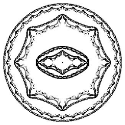
Figure 1: The Julia set of $G=\langle g_{1}^{2},g_{2}^{2}\rangle$, where $g_{1}(z):=z^{2}-1,g_{2}(z):=\frac{z^{2}}{4}.$ For a.e.$\gamma$, $J_{\gamma}(f)$ is a Jordan curve but not a quasicircle, $A_{\gamma}(f)$ is a John domain, and the bounded component of $F_{\gamma}(f)$ is not a John domain. For each connected component $J$ of $J(G)$, there exists a unique $\gamma\in\Gamma^{\mathbb{N}}$ such that $J=J_{\gamma}(f).$

Example 2.23.

Let $h_{1}(z):=z^{2}-1$ and $h_{2}(z):=az^{2}$, where $a\in\mathbb{C}$ with $0<|a|<0.1.$ Let $\Gamma:=\{h_{1},h_{2}\}.$ Moreover, let $G:=\langle h_{1},h_{2}\rangle.$ Let $U:=\{|z|<0.2\}.$ Then, it is easy to see that $h_{2}(U)\subset U,\ h_{2}(h_{1}(U))\subset U,$ and $h_{1}^{2}(U)\subset U.$ Hence, $U\subset F(G).$ It follows that $P^{\ast}(G)\subset$ int$(\hat{K}(G))\subset F(G).$ Therefore, $G\in{\cal G}$ and $G$ is hyperbolic. Since $J(h_{1})$ is not a Jordan curve and $J(h_{2})$ is a Jordan curve, Theorem 2.21 implies that there exists a residual subset ${\cal U}$ of $\Gamma^{\mathbb{N}}$ such that, for each Borel probability measure $\tau$ on Poly_deg≥2 with $\Gamma_{\tau}=\Gamma$, we have $\tilde{\tau}({\cal U})=1$, and such that, for each $\gamma\in{\cal U}$, $J_{\gamma}(f)$ is a Jordan curve but not a quasicircle. Moreover, for each $\gamma\in{\cal U}$, $A_{\gamma}(f)$ is a John domain, but the bounded component of $F_{\gamma}(f)$ is not a John domain.

Remark 2.24.

Let $h\in$ Poly_deg≥2 be a polynomial. Suppose that $J(h)$ is a Jordan curve but not a quasicircle. Then, it is easy to see that there exists a parabolic fixed point of $h$ in $\mathbb{C}$ and the bounded connected component of $F(h)$ is the immediate parabolic basin. Hence, $\langle h\rangle$ is not semi-hyperbolic. Moreover, by [5], $F_{\infty}(h)$ is not a John domain.

Thus what we see in statement 2 in Theorem 2.19 and statement 2 in Theorem 2.21, as illustrated in Example  2.22 and Example 2.23 (see also Section 5), is a phenomenon which can hold in the random dynamics of a family of polynomials, but cannot hold in the usual iteration dynamics of a single polynomial. Namely, it can hold that for almost every $\gamma\in\Gamma^{\mathbb{N}}$, $J_{\gamma}(f)$ is a Jordan curve and fails to be a quasicircle all while the basin of infinity $A_{\gamma}(f)$ is still a John domain. Whereas, if $J(h)$, for some polynomial $h$, is a Jordan curve which fails to be a quasicircle, then the basin of infinity $F_{\infty}(h)$ is necessarily not a John domain.

In Section 5, we will see how easily situation 2 in Theorem 2.19 and situation 2 in Theorem 2.21 occur.

Pilgrim and Tan Lei ([18]) showed that there exists a hyperbolic rational map $h$ with disconnected Julia set such that “almost every” connected component of $J(h)$ is a Jordan curve but not a quasicircle.

We give a sufficient condition so that statement 1 in Theorem 2.21 holds.

Proposition 2.25.

Let $\Gamma$ be a non-empty compact subset of Poly${}_{\deg\geq 2}.$ Let $f:\Gamma^{\mathbb{N}}\times\hat{\mathbb{C}}\rightarrow\Gamma^{\mathbb{N}}\times\hat{\mathbb{C}}$ be the skew product associated with the family $\Gamma.$ Let $G$ be the polynomial semigroup generated by $\Gamma.$ Suppose that $P^{\ast}(G)$ is included in a connected component of int$(\hat{K}(G)).$ Then, there exists a constant $K\geq 1$ such that for each $\gamma\in\Gamma^{\mathbb{N}}$, $J_{\gamma}(f)$ is a $K$-quasicircle.

Example 2.26.

Let $d_{1},\ldots,d_{m}\in\mathbb{N}$ with $d_{j}\geq 2$ for each $j$, and let $h_{j}(z)=a_{j}z^{d_{j}}+c_{j},a_{j}\neq 0,$ for each $j=1,\ldots,m.$ Let $\Gamma=\langle g_{1},\ldots,g_{m}\rangle.$ If $|c_{j}|$ is small enough for each $j$, then $\Gamma$ satisfies the assumption of Proposition 2.25. Thus statement 1 in Theorem 2.21 holds.

We have also many examples of $\Gamma$ such that statement 3 in Theorem 2.19 or statement 3 in Theorem 2.21 holds.

Example 2.27.

Let $h_{1}\in\mbox{Poly}_{\deg\geq 2}.$ Suppose that $\langle h_{1}\rangle\in{\cal G}$ and $h_{1}$ is hyperbolic. Suppose also that $h_{1}$ has at least two attracting periodic points in $\mathbb{C}.$ Let $\Gamma$ be a small compact neighborhood of $h_{1}$ in Poly${}_{\deg\geq 2}.$ Then $\langle\Gamma\rangle\in{\cal G}$ and $\langle\Gamma\rangle$ is hyperbolic (see Lemma 5.4). Moreover, by the argument in the proof of Lemma 5.6, we see that for each $\gamma\in\Gamma^{\mathbb{N}}$, $F_{\gamma}(f)$ has at least two bounded connected components, where $f:\Gamma^{\mathbb{N}}\times\hat{\mathbb{C}}\rightarrow\Gamma^{\mathbb{N}}\times\hat{\mathbb{C}}$ is the skew product associated with $\Gamma$. Thus statement 3 in Theorem 2.21 holds. We remark that by using Lemma 5.5, 5.6 and their proofs, we easily obtain many examples of $\Gamma$ such that statement 3 in Theorem 2.19 or statement 3 in Theorem 2.21 holds.

3 Tools

To show the main results, we need some tools in this section.

3.1 Fundamental properties of rational semigroups

Notation: For a rational semigroup $G$, we set $E(G):=\{z\in\hat{\mathbb{C}}\mid\sharp(\bigcup_{g\in G}g^{-1}(\{z\}))<\infty\}.$ This is called the exceptional set of $G.$
Notation: Let $r>0.$ For a subset $A$ of $\hat{\mathbb{C}}$, we set $B(A,r):=\{z\in\hat{\mathbb{C}}\mid d_{s}(z,A)<r\}$, where $d_{s}$ is the spherical distance. For a subset $A$ of $\mathbb{C}$, we set $D(A,r):=\{z\in\mathbb{C}\mid d_{e}(z,A)<r\}$, where $d_{e}$ is the Euclidean distance.

We use the following Lemma 3.1 and Theorem 3.2 in the proofs of the main results.

Lemma 3.1 ([12, 11, 29, 27]).

Let $G$ be a rational semigroup.

1. For each $h\in G,\$ we have $h(F(G))\subset F(G)$ and $h^{-1}(J(G))\subset J(G).$ Note that we do not have that the equality holds in general.

2. If $G=\langle h_{1},\ldots,h_{m}\rangle$, then $J(G)=h_{1}^{-1}(J(G))\cup\cdots\cup h_{m}^{-1}(J(G)).$ More generally, if $G$ is generated by a compact subset $\Gamma$ of Rat, then $J(G)=\bigcup_{h\in\Gamma}h^{-1}(J(G)).$ (We call this property of the Julia set of a compactly generated rational semigroup “backward self-similarity.” )

3. If $\sharp(J(G))\geq 3$ , then $J(G)$ is a perfect set.

4. If $\sharp(J(G))\geq 3$ , then $\sharp(E(G))\leq 2.$

5. If a point $z$ is not in $E(G),\$ then $J(G)\subset\overline{\bigcup_{g\in G}g^{-1}(\{z\})}.$ In particular if a point $z$ belongs to  $J(G)\setminus E(G),$  then $\overline{\bigcup_{g\in G}g^{-1}(\{z\})}=J(G).$

6. If $\sharp(J(G))\geq 3$ , then $J(G)$ is the smallest closed backward invariant set containing at least three points. Here we say that a set $A$ is backward invariant under $G$ if for each $g\in G,\ g^{-1}(A)\subset A.\$

Theorem 3.2 ([12, 11, 29]).

Let $G$ be a rational semigroup. If $\sharp(J(G))\geq 3$, then
$J(G)=\overline{\{z\in\mathbb{C}\mid\exists g\in G,\ g(z)=z,\ |g^{\prime}(z)|>1\}}$, where the closure is taken in $\hat{\mathbb{C}}.$ In particular, $J(G)=\overline{\bigcup_{g\in G}J(g)}.$

Remark 3.3.

If a rational semigroup $G$ contains an element $g$ with $\deg(g)\geq 2$, then $\sharp(J(g))\geq 3$, which implies that $\sharp(J(G))\geq 3.$

3.2 Fundamental properties of fibered rational maps

Lemma 3.4.

Let $f:X\times\hat{\mathbb{C}}\rightarrow X\times\hat{\mathbb{C}}$ be a rational skew product over $g:X\rightarrow X.$ Then, we have the following.

1. ([27, Lemma 2.4]) For each $x\in X$, $(f_{x,1})^{-1}(J_{g(x)}(f))=J_{x}(f).$ Furthermore, we have $\hat{J}_{x}(f)\supset J_{x}(f).$ Note that equality $\hat{J_{x}}(f)=J_{x}(f)$ does not hold in general.

   If $g:X\rightarrow X$ is a surjective and open map, then $f^{-1}(\tilde{J}(f))=\tilde{J}(f)=f(\tilde{J}(f))$, and for each $x\in X$, $(f_{x,1})^{-1}(\hat{J}_{g(x)}(f))=\hat{J}_{x}(f).$

2. ([14, 27]) If $d(x)\geq 2$ for each $x\in X$, then for each $x\in X$, $J_{x}(f)$ is a non-empty perfect set with $\sharp(J_{x}(f))\geq 3.$ Furthermore, the map $x\mapsto J_{x}(f)$ is lower semicontinuous; i.e., for any point $(x,y)\in X\times\hat{\mathbb{C}}$ with $y\in J_{x}(f)$ and any sequence $\{x^{n}\}_{n\in\mathbb{N}}$ in $X$ with $x^{n}\rightarrow x,\$ there exists a sequence $\{y^{n}\}_{n\in\mathbb{N}}$ in $\hat{\mathbb{C}}$ with $y^{n}\in J_{x^{n}}(f)$ for each $n\in\mathbb{N}$ such that $y^{n}\rightarrow y.$ However, $x\mapsto J_{x}(f)$ is not continuous with respect to the Hausdorff topology in general.

3. If $d(x)\geq 2$ for each $x\in X$, then $\inf_{x\in X}$diam${}_{S}J_{x}(f)>0$, where diam_S denotes the diameter with respect to the spherical distance.

4. If $f:X\times\hat{\mathbb{C}}\rightarrow X\times\hat{\mathbb{C}}$ is a polynomial skew product and $d(x)\geq 2$ for each $x\in X$, then there exists a ball $B$ around $\infty$ such that for each $x\in X$, $B\subset A_{x}(f)\subset F_{x}(f)$, and for each $x\in X$, $J_{x}(f)=\partial K_{x}(f)=\partial A_{x}(f).$ Moreover, for each $x\in X$, $A_{x}(f)$ is connected.

5. If $f:X\times\hat{\mathbb{C}}\rightarrow X\times\hat{\mathbb{C}}$ is a polynomial skew product and $d(x)\geq 2$ for each $x\in X$, and if $\omega\in X$ is a point such that int$(K_{w}(f))$ is a non-empty set, then $\overline{\mbox{{\em int}}(K_{\omega}(f))}=K_{\omega}(f)$ and $\partial(\mbox{{\em int}}(K_{\omega}(f)))=J_{\omega}(f).$

Proof.

For the proof of statement 1, see [27, Lemma 2.4]. For the proof of statement 2, see [14] and [27].

By statement 2, it is easy to see that statement 3 holds. Moreover, it is easy to see that statement 4 holds.

To show statement 5, let $y\in J_{\omega}(f)$ be a point. Let $V$ be an arbitrary neighborhood of $y$ in $\hat{\mathbb{C}}.$ Then, by the self-similarity of Julia sets (see [3]), there exists an $n\in\mathbb{N}$ such that $f_{\omega,n}(V\cap J_{\omega}(f))=J_{g^{n}(\omega)}(f).$ Since $\partial(\mbox{int}(K_{g^{n}(\omega)}(f)))\subset J_{g^{n}(\omega)}(f)$ and $(f_{\omega,n})^{-1}(K_{g^{n}(\omega)}(f))=K_{\omega}(f)$, it follows that $V\cap\partial(\mbox{int}(K_{\omega}(f)))\neq\emptyset.$ Hence, we obtain $J_{\omega}(f)=\partial(\mbox{int}(K_{\omega}(f)).$ Therefore, we have proved statement 5. ∎

Lemma 3.5.

Let $f:\Gamma^{\mathbb{N}}\times\hat{\mathbb{C}}\rightarrow\Gamma^{\mathbb{N}}\times\hat{\mathbb{C}}$ be a skew product associated with a compact subset $\Gamma$ of Rat. Let $G$ be the rational semigroup generated by $\Gamma.$ Suppose that $\sharp(J(G))\geq 3.$ Then, we have the following.

1. $\pi_{\hat{\mathbb{C}}}(\tilde{J}(f))=J(G).$

2. For each $\gamma=(\gamma_{1},\gamma_{2},\ldots,)\in\Gamma^{\mathbb{N}}$, $\hat{J}_{\gamma}(f)=\bigcap_{j=1}^{\infty}\gamma_{1}^{-1}\cdots\gamma_{j}^{-1}(J(G)).$

Proof.

First, we show statement 1. Since $J_{\gamma}(f)\subset J(G)$ for each $\gamma\in\Gamma$, we have $\pi_{\hat{\mathbb{C}}}(\tilde{J}(f))\subset J(G).$ By Theorem 3.2, we have $J(G)=\overline{\bigcup_{g\in G}J(g)}.$ Since $\bigcup_{g\in G}J(g)\subset\pi_{\hat{\mathbb{C}}}(\tilde{J}(f))$, we obtain $J(G)\subset\pi_{\hat{\mathbb{C}}}(\tilde{J}(f)).$ Therefore, we obtain $\pi_{\hat{\mathbb{C}}}(\tilde{J}(f))=J(G).$

We now show statement 2. Let $\gamma=(\gamma_{1},\gamma_{2},\ldots)\in\Gamma^{\mathbb{N}}.$ By statement 1 in Lemma 3.4, we see that for each $j\in\mathbb{N}$, $\gamma_{j}\cdots\gamma_{1}(\hat{J}_{\gamma}(f))=\hat{J}_{\sigma^{j}(\gamma)}(f)\subset J(G).$ Hence, $\hat{J}_{\gamma}(f)\subset\bigcap_{j=1}^{\infty}\gamma_{1}^{-1}\cdots\gamma_{j}^{-1}(J(G)).$ Suppose that there exists a point $(\gamma,y)\in\Gamma^{\mathbb{N}}\times\hat{\mathbb{C}}$ such that $y\in$ $\left(\bigcap_{j=1}^{\infty}\gamma_{1}^{-1}\cdots\gamma_{j}^{-1}(J(G))\right)\setminus\hat{J}_{\gamma}(f).$ Then, we have $(\gamma,y)\in(\Gamma^{\mathbb{N}}\times\hat{\mathbb{C}})\setminus\tilde{J}(f).$ Hence, there exists a neighborhood $U$ of $\gamma$ in $\Gamma^{\mathbb{N}}$ and a neighborhood $V$ of $y$ in $\hat{\mathbb{C}}$ such that $U\times V\subset\tilde{F}(f).$ Then, there exists an $n\in\mathbb{N}$ such that $\{\rho\in\Gamma^{\mathbb{N}}\mid\rho_{j}=\gamma_{j},j=1,\ldots,n\}\subset U.$ Combining it with Lemma 3.4-1, we obtain $\tilde{F}(f)\supset f^{n}(U\times V)\supset\Gamma^{\mathbb{N}}\times\{f_{\gamma,n}(y)\}.$ Moreover, since we have $f_{\gamma,n}(y)\in J(G)=\pi_{\hat{\mathbb{C}}}(\tilde{J}(f))$, where the last equality holds by statement 1, we get that there exists an element $\gamma^{\prime}\in\Gamma^{\mathbb{N}}$ such that $(\gamma^{\prime},f_{\gamma,n}(y))\in\tilde{J}(f).$ However, it contradicts $(\gamma^{\prime},f_{\gamma,n}(y))\in\Gamma^{\mathbb{N}}\times\{f_{\gamma,n}(y)\}\subset\tilde{F}(f).$ Hence, we obtain $\hat{J}_{\gamma}(f)=\bigcap_{j=1}^{\infty}\gamma_{1}^{-1}\cdots\gamma_{j}^{-1}(J(G)).$ ∎

Lemma 3.6.

Let $f:X\times\hat{\mathbb{C}}\rightarrow X\times\hat{\mathbb{C}}$ be a polynomial skew product over $g:X\rightarrow X$ such that for each $x\in X$, $d(x)\geq 2.$ Then, the following are equivalent.

1. $\pi_{\hat{\mathbb{C}}}(P(f))\setminus\{\infty\}$ is bounded in $\mathbb{C}.$

2. For each $x\in X$, $J_{x}(f)$ is connected.

3. For each $x\in X$, $\hat{J}_{x}(f)$ is connected.

Proof.

First, we show 1 $\Rightarrow$2. Suppose that 1 holds. Let $R>0$ be a number such that for each $x\in X$, $B:=\{y\in\hat{\mathbb{C}}\mid|y|>R\}\subset A_{x}(f)$ and $\overline{f_{x,1}(B)}\subset B.$ Then, for each $x\in X$, we have $A_{x}(f)=\bigcup_{n\in\mathbb{N}}(f_{x,n})^{-1}(B)$ and $(f_{x,n})^{-1}(B)\subset(f_{x,n+1})^{-1}(B)$, for each $n\in\mathbb{N}.$ Furthermore, since we assume 1, we see that for each $n\in\mathbb{N}$, $(f_{x,n})^{-1}(B)$ is a simply connected domain, by the Riemann-Hurwitz formula. Hence, for each $x\in X$, $A_{x}(f)$ is a simply connected domain. Since $\partial A_{x}(f)=J_{x}(f)$ for each $x\in X,$ we conclude that for each $x\in X$, $J_{x}(f)$ is connected. Hence, we have shown 1 $\Rightarrow$ 2.

Next, we show 2 $\Rightarrow$ 3. Suppose that 2 holds. Let $z_{1}\in\hat{J}_{x}(f)$ and $z_{2}\in J_{x}(f)$ be two points. Let $\{x^{n}\}_{n\in\mathbb{N}}$ be a sequence such that $x^{n}\rightarrow x$ as $n\rightarrow\infty$, and such that $d(z_{1},J_{x^{n}}(f))\rightarrow 0$ as $n\rightarrow\infty.$ We may assume that there exists a non-empty compact set $K$ in $\hat{\mathbb{C}}$ such that $J_{x^{n}}(f)\rightarrow K$ as $n\rightarrow\infty$, with respect to the Hausdorff topology in the space of non-empty compact sets in $\hat{\mathbb{C}}.$ Since we assume 2, $K$ is connected. By Lemma 3.4-2, we have $d(z_{2},J_{x^{n}}(f))\rightarrow 0$ as $n\rightarrow\infty.$ Hence, $z_{i}\in K$ for each $i=1,2.$ Therefore, $z_{1}$ and $z_{2}$ belong to the same connected component of $\hat{J}_{x}(f).$ Thus, we have shown 2 $\Rightarrow$ 3.

Next, we show 3 $\Rightarrow$ 1. Suppose that 3 holds. It is easy to see that $A_{x}(f)\cap\hat{J}_{x}(f)=\emptyset$ for each $x\in X.$ Hence, $A_{x}(f)$ is a connected component of $\hat{\mathbb{C}}\setminus\hat{J}_{x}(f).$ Since we assume 3, we have that for each $x\in X$, $A_{x}(f)$ is a simply connected domain. Since $(f_{x,1})^{-1}(A_{g(x)}(f))=A_{x}(f)$, the Riemann-Hurwitz formula implies that for each $x\in X$, there exists no critical point of $f_{x,1}$ in $A_{x}(f)\cap\mathbb{C}.$ Therefore, we obtain 1. Thus, we have shown 3 $\Rightarrow$ 1. ∎

Corollary 3.7.

Let $G=\langle h_{1},h_{2}\rangle\in{\cal G}.$ Then, $h_{1}^{-1}(J(h_{2}))$ is connected.

Proof.

Let $f:\Gamma^{\mathbb{N}}\times\hat{\mathbb{C}}\rightarrow\Gamma^{\mathbb{N}}\times\hat{\mathbb{C}}$ be the skew product associated with the family $\Gamma=\{h_{1},h_{2}\}.$ Let $\gamma=(h_{1},h_{2},h_{2},h_{2},h_{2},\ldots)\in\Gamma^{\mathbb{N}}.$ Then, by Lemma 3.4-1, we have $J_{\gamma}(f)=h_{1}^{-1}(J(h_{2})).$ From Lemma 3.6, it follows that $h_{1}^{-1}(J(h_{2}))$ is connected. ∎

Lemma 3.8.

Let $G$ be a polynomial semigroup generated by a compact subset $\Gamma$ of Poly${}_{\deg\geq 2}.$ Let $f:\Gamma^{\mathbb{N}}\times\hat{\mathbb{C}}\rightarrow\Gamma^{\mathbb{N}}\times\hat{\mathbb{C}}$ be the skew product associated with the family $\Gamma.$ Suppose that $G\in{\cal G}.$ Then for each $\gamma=(\gamma_{1},\gamma_{2},\ldots,)\in\Gamma^{\mathbb{N}}$, the sets $J_{\gamma}(f),\ \hat{J}_{\gamma}(f)$, and $\bigcap_{j=1}^{\infty}\gamma_{1}^{-1}\cdots\gamma_{j}^{-1}(J(G))$ are connected.

Proof.

From Lemma 3.5-2 and Lemma 3.6, the lemma follows. ∎

Lemma 3.9.

Under the same assumption as that in Lemma 3.8, let $\gamma,\rho\in\Gamma^{\mathbb{N}}$ be two elements with $J_{\gamma}(f)\cap J_{\rho}(f)=\emptyset.$ Then, either $J_{\gamma}(f)<J_{\rho}(f)$ or $J_{\rho}(f)<J_{\gamma}(f).$

Proof.

Let $\gamma,\rho\in\Gamma^{\mathbb{N}}$ with $J_{\gamma}(f)\cap J_{\rho}(f)=\emptyset.$ Suppose that the statement “either $J_{\gamma}(f)<J_{\rho}(f)$ or $J_{\rho}(f)<J_{\gamma}(f)$” is not true. Then, Lemma 3.6 implies that $J_{\gamma}(f)$ is included in the unbounded component of $\mathbb{C}\setminus J_{\rho}(f)$, and that $J_{\rho}(f)$ is included in the unbounded component of $\mathbb{C}\setminus J_{\gamma}(f).$ From Lemma 3.4-4, it follows that $K_{\rho}(f)$ is included in the unbounded component $A_{\gamma}(f)\setminus\{\infty\}$ of $\mathbb{C}\setminus J_{\gamma}(f).$ However, it causes a contradiction, since $\emptyset\neq P^{\ast}(G)\subset\hat{K}(G)\subset K_{\rho}(f)\cap K_{\gamma}(f).$ ∎

Definition 3.10.

Let $f:\Gamma^{\mathbb{N}}\times\hat{\mathbb{C}}\rightarrow\Gamma^{\mathbb{N}}\times\hat{\mathbb{C}}$ be a polynomial skew product over $g:X\rightarrow X.$ Let $p\in\mathbb{C}$ and $\epsilon>0.$ We set
${\cal F}_{f,p,\epsilon}:=\{\alpha:D(p,\epsilon)\rightarrow\mathbb{C}\mid\alpha\mbox{ is a well-defined branch of }(f_{x,n})^{-1},x\in X,n\in\mathbb{N}\}.$

Lemma 3.11.

Let $f:\Gamma^{\mathbb{N}}\times\hat{\mathbb{C}}\rightarrow\Gamma^{\mathbb{N}}\times\hat{\mathbb{C}}$ be a polynomial skew product over $g:X\rightarrow X$ such that for each $x\in X$, $d(x)\geq 2.$ Let $R>0,\epsilon>0$, and
${\cal F}:=\{\alpha\circ\beta:D(0,1)\rightarrow\mathbb{C}\mid\beta:D(0,1)\cong D(p,\epsilon),\ \alpha:D(p,\epsilon)\rightarrow\mathbb{C},\ \alpha\in{\cal F}_{f,p,\epsilon},\ p\in D(0,R)\}.$ Then, ${\cal F}$ is normal in $D(0,1).$

Proof.

Since $d(x)\geq 2$ for each $x\in X$, there exists a ball $B$ around $\infty$ with $B\subset\hat{\mathbb{C}}\setminus D(0,R+\epsilon)$ such that for each $x\in X$, $f_{x,1}(B)\subset B.$ Let $p\in D(0,R).$ Then, for each $\alpha\in{\cal F}_{f,p,\epsilon}$, $\alpha(D(p,\epsilon))\subset\hat{\mathbb{C}}\setminus B.$ Hence, ${\cal F}$ is normal in $D(0,1).$ ∎

Definition 3.12.

For a polynomial semigroup $G$ with $\infty\in F(G)$, we denote by $F_{\infty}(G)$ the connected component of $F(G)$ containing $\infty.$ Moreover, for a polynomial $g$ with $\deg(g)\geq 2$, we set $F_{\infty}(g):=F_{\infty}(\langle g\rangle).$ (Note that if $\Gamma$ is a non-empty compact subset of Poly_deg≥2, then $\infty\in F(\langle\Gamma\rangle).$)

Lemma 3.13.

Let $G$ be a polynomial semigroup generated by a compact subset $\Gamma$ of Poly${}_{\deg\geq 2}.$ If a sequence $\{g_{n}\}_{n\in\mathbb{N}}$ of elements of $G$ tends to a constant $w_{0}\in\hat{\mathbb{C}}$ locally uniformly on a domain $V\subset\hat{\mathbb{C}}$, then $w_{0}\in P(G).$

Proof.

Since $\infty\in P(G)$, we may assume that $w_{0}\in\mathbb{C}.$ Suppose $w_{0}\in\mathbb{C}\setminus P(G).$ Then, there exists a $\delta>0$ such that $B(w_{0},2\delta)\subset\mathbb{C}\setminus P(G).$ Let $z_{0}\in V$ be a point. Then, for each large $n\in\mathbb{N}$, there exists a well-defined branch $\alpha_{n}$ of $g_{n}^{-1}$ on $B(w_{0},2\delta)$ such that $\alpha_{n}(g_{n}(z_{0}))=z_{0}.$ Let $B:=B(w_{0},\delta).$ Since $\Gamma$ is compact, there exists a connected component $F_{\infty}(G)$ of $F(G)$ containing $\infty.$ Let $C$ be a compact neighborhood of $\infty$ in $F_{\infty}(G).$ Then, we must have that there exists a number $n_{0}$ such that $\alpha_{n}(B)\cap C=\emptyset$ for each $n\geq n_{0}$, since $g_{n}\rightarrow\infty$ uniformly on $C$ as $n\rightarrow\infty$, which follows from that $\deg(g_{n})\rightarrow\infty$ and local degree at $\infty$ of $g_{n}$ tends to $\infty$ as $n\rightarrow\infty.$ Hence, $\{\alpha_{n}|_{B}\}_{n\geq n_{0}}$ is normal in $B.$ However, for a small $\epsilon$ so that $B(z_{0},2\epsilon)\subset V$, we have $g_{n}(B(z_{0},\epsilon))\rightarrow w_{0}$ as $n\rightarrow\infty$, and this is a contradiction. Hence, we must have that $w_{0}\in P(G).$ ∎

4 Proofs of the main results

In this section, we demonstrate the main results.

We first need the following.

Theorem 4.1.

(Uniform fiberwise quasiconformal surgery) Let $f:X\times\hat{\mathbb{C}}\rightarrow X\times\hat{\mathbb{C}}$ be a polynomial skew product over $g:X\rightarrow X$ such that for each $x\in X$, $d(x)\geq 2.$ Suppose that $f$ is hyperbolic and that $\pi_{\hat{\mathbb{C}}}(P(f))\setminus\{\infty\}$ is bounded in $\mathbb{C}.$ Moreover, suppose that for each $x\in X$, int$(K_{x}(f))$ is connected. Then, there exists a constant $K$ such that for each $x\in X,\ J_{x}(f)$ is a $K$-quasicircle.

Proof.

Step 1: By [27, Theorem 2.14-(4)], the map $x\mapsto J_{x}(f)$ is continuous with respect to the Hausdorff topology. Hence, there exists a positive constant $C_{1}$ such that, for each $x\in X,\ \inf\{d(a,b)\mid a\in J^{x}(f),\ b\in\pi^{-1}(\{x\})\cap P^{\ast}(f)\}>C_{1}$, where $P^{\ast}(f):=P(f)\setminus\pi_{\hat{\mathbb{C}}}^{-1}(\{\infty\})$, and $d(\cdot,\cdot)$ denotes the spherical distance, under the canonical identification $\pi^{-1}(\{x\})\cong\hat{\mathbb{C}}.$ Moreover, from the assumption, we have that, for each $x\in X$, int$(K_{x}(f))\neq\emptyset.$ Since $X$ is compact, it follows that, for each $x\in X,$ there exists an analytic Jordan curve $\zeta_{x}$ in $K^{x}(f)\cap F^{x}(f)$ such that:

1. $\pi^{-1}(\{x\})\cap P^{\ast}(f)$ is included in the bounded component $V_{x}$ of $\pi^{-1}(\{x\})\setminus\zeta_{x}$;

2. $\inf_{z\in\zeta_{x}}d(z,\ J^{x}(f)\cup(\pi^{-1}(\{x\})\cap P^{\ast}(f)))\geq C_{2}$, where $C_{2}$ is a positive constant independent of $x\in X$; and

3. there exist finitely many Jordan curves $\xi_{1},\ldots,\xi_{k}$ in $\mathbb{C}$ such that for each $x\in X$, there exists a $j$ with $\pi_{\hat{\mathbb{C}}}(\zeta_{x})=\xi_{j}.$

Step 2: By [30, Corollary 2.7], there exists an $n\in\mathbb{N}$ such that for each $x\in X,\ W_{x}:=(f_{x}^{n})^{-1}(V_{g^{n}(x)})\supset\overline{V_{x}}$, $\inf\{d(a,b)\mid a\in\partial W_{x},b\in\partial V_{x},x\in X\}>0$, and mod $(W_{x}\setminus\overline{V_{x}})\geq C_{3},$ where $C_{3}$ is a positive constant independent of $x\in X.$ In order to prove the theorem, since $J_{x}(f^{n})=J_{x}(f)$ for each $x\in X$, replacing $f:X\times\hat{\mathbb{C}}\rightarrow X\times\hat{\mathbb{C}}$ by $f^{n}:X\times\hat{\mathbb{C}}\rightarrow X\times\hat{\mathbb{C}}$, we may assume $n=1.$

Step 3: For each $x\in X$, let $\varphi_{x}:\pi^{-1}(\{x\})\setminus\overline{V_{x}}\rightarrow\pi^{-1}(\{x\})\setminus\overline{D(0,\frac{1}{2})}$ be a biholomorphic map such that $\varphi_{x}(x,\infty)=(x,\infty),$ under the canonical identification $\pi^{-1}(\{x\})\cong\hat{\mathbb{C}}.$ We see that $\varphi_{x}$ extends analytically over $\partial V_{x}=\zeta_{x}.$ For each $x\in X$, we define a quasi-regular map $h_{x}:\pi^{-1}(\{x\})\cong\hat{\mathbb{C}}\rightarrow\pi^{-1}(\{g(x)\})\cong\hat{\mathbb{C}}$ as follows:

$$h_{x}(z):=\begin{cases}\varphi_{g(x)}f_{x}\varphi_{x}^{-1}(z),\ \mbox{ if }z\in\varphi_{x}(\pi^{-1}(\{x\})\setminus W_{x}),\\ z^{d(x)},\ \mbox{ if }z\in\overline{D(0,\frac{1}{2})},\\ \tilde{h}_{x}(z),\ \mbox{\ if }z\in\varphi_{x}(W_{x}\setminus\overline{V_{x}}),\end{cases}$$

where $\tilde{h}_{x}:\varphi_{x}(W_{x}\setminus\overline{V_{x}})\rightarrow D(0,\frac{1}{2})\setminus\overline{D(0,(\frac{1}{2})^{d(x)})}$ is a regular covering and a $K_{0}$-quasiregular map with dilatation constant $K_{0}$ independent of $x\in X.$

Step 4: For each $x\in X$, we define a Beltrami differential $\mu_{x}(z)\frac{d\overline{z}}{dz}$ on $\pi^{-1}(\{x\})\cong\hat{\mathbb{C}}$ as follows:

$$\begin{cases}\frac{\partial_{\overline{z}}\tilde{h}_{x}}{\partial_{z}\tilde{h}_{x}}\frac{d\overline{z}}{dz},\ \mbox{ if }z\in\varphi_{x}(W_{x}\setminus\overline{V_{x}}),\\ (h_{g^{m-1}(x)}\cdots h_{x})^{\ast}(\frac{\partial_{\overline{z}}\tilde{h}_{g^{m}(x)}}{\partial_{z}\tilde{h}_{g^{m}(x)}}\frac{d\overline{z}}{dz}),\ \mbox{ if }z\in(h_{g^{m-1}(x)}\cdots h_{x})^{-1}(\varphi_{g^{m}(x)}(W_{g^{m}(x)}\setminus\overline{V_{g^{m}(x)}})),\\ 0,\ \ \ \mbox{otherwise.}\end{cases}$$

Then, there exists a constant $k$ with $0<k<1$ such that for each $x\in X,\ \|\mu_{x}\|_{\infty}\leq k.$ By the construction, we have $h_{x}^{\ast}(\mu_{g(x)}\frac{d\overline{z}}{dz})=\mu_{x}\frac{d\overline{z}}{dz}$, for each $x\in X.$ By the measurable Riemann mapping theorem ([15, page 194]), for each $x\in X$, there exists a quasiconformal map $\psi_{x}:\pi^{-1}(\{x\})\rightarrow\pi^{-1}(\{x\})$ such that $\partial_{\overline{z}}\psi_{x}=\mu_{x}\partial_{z}\psi_{x},\ \psi_{x}(0)=0,\ \psi_{x}(1)=1,$ and $\psi_{x}(\infty)=\infty$, under the canonical identification $\pi^{-1}(\{x\})\cong\hat{\mathbb{C}}.$ For each $x\in X$, let $\hat{h}_{x}:=\psi_{g(x)}h_{x}\psi_{x}^{-1}:\pi^{-1}(\{x\})\rightarrow\pi^{-1}(\{g(x)\}).$ Then, $\hat{h}_{x}$ is holomorphic on $\pi^{-1}(\{x\}).$ By the construction, we see that $\hat{h}_{x}(z)=c(x)z^{d(x)}$, where $c(x)=\psi_{g(x)}h_{x}\psi_{x}^{-1}(1)=\psi_{g(x)}h_{x}(1).$ Moreover, by the construction again, we see that there exists a positive constant $C_{4}$ such that for each $x\in X,\ \frac{1}{C_{4}}\leq|h_{x}(1)|\leq C_{4}.$ Furthermore, [15, Theorem 5.1 in page 73] implies that under the canonical identification $\pi^{-1}(\{x\})\cong\hat{\mathbb{C}}$, the family $\{\psi_{x}^{-1}\}_{x\in X}$ is normal in $\hat{\mathbb{C}}.$ Therefore, it follows that there exists a positive constant $C_{5}$ such that for each $x\in X,\ \frac{1}{C_{5}}\leq|c(x)|\leq C_{5}.$ Let $\tilde{J}_{x}$ be the set of non-normality of the sequence $\{\hat{h}_{g^{m}(x)}\cdots\hat{h}_{x}\}_{m\in\mathbb{N}}$ in $\pi^{-1}(\{x\})\cong\hat{\mathbb{C}}.$ Since $\hat{h}_{x}(z)=c(x)z^{d(x)}$ and $\frac{1}{C_{5}}\leq|c(x)|\leq C_{5}$ for each $x\in X$, we get that for each $x\in X$, $\tilde{J}_{x}$ is a round circle. Moreover, [15, Theorem 5.1 in page 73] implies that $\{\psi_{x}\}_{x\in X}$ and $\{\psi_{x}^{-1}\}_{x\in X}$ are normal in $\hat{\mathbb{C}}$ (under the canonical identification $\pi^{-1}(\{x\})\cong\hat{\mathbb{C}}$). Combining it with [30, Corollary 2.7], we see that for each $x\in X$, $J^{x}(f)=\varphi_{x}^{-1}(\psi_{x}^{-1}(\tilde{J}_{x}))$, and it follows that there exists a constant $K$ such that for each $x\in X,\ J_{x}(f)$ is a $K$-quasicircle.

Thus, we have proved Theorem 4.1. ∎

Remark 4.2.

Theorem 4.1 generalizes a result in [19, THÉORÈME 5.2], where O. Sester investigated hyperbolic polynomial skew products $f:X\times\hat{\mathbb{C}}\rightarrow X\times\hat{\mathbb{C}}$ such that for each $x\in X$, $d(x)=2.$

We next need the notion of (fiberwise) external rays.

Definition 4.3.

Let $h$ be a polynomial with $\deg(h)\geq 2.$ Suppose that $J(h)$ is connected. Let $\psi$ be a biholomorphic map $\hat{\mathbb{C}}\setminus\overline{D(0,1)}\rightarrow F_{\infty}(h)$ with $\psi(\infty)=\infty$ such that $\psi^{-1}\circ h\circ\psi(z)=z^{\deg(h)}$, for each $z\in\hat{\mathbb{C}}\setminus\overline{D(0,1)}.$ (For the existence of the biholomorphic map $\psi$, see [16, Theorem 9.5].) For each $\theta\in\partial D(0,1)$, we set $T(\theta):=\psi(\{r\theta\mid 1<r\leq\infty\}).$ This is called the external ray (for $K(h)$) with angle $\theta.$

Lemma 4.4.

Let $f:X\times\hat{\mathbb{C}}\rightarrow X\times\hat{\mathbb{C}}$ be a polynomial skew product over $g:X\rightarrow X$ such that for each $x\in X$, $d(x)\geq 2.$ Let $\gamma\in X$ be a point. Suppose that $J_{\gamma}(f)$ is a Jordan curve. Then, for each $n\in\mathbb{N}$, $J_{g^{n}(\gamma)}(f)$ is a Jordan curve. Moreover, for each $n\in\mathbb{N}$, there exists no critical value of $f_{\gamma,n}$ in $J_{g^{n}(\gamma)}(f).$

Proof.

Since $(f_{\gamma,1})^{-1}(K_{g(\gamma)}(f))=K_{\gamma}(f)$, it follows that int$(K_{g(\gamma)}(f))$ is a non-empty connected set. Moreover, $J_{g(\gamma)}(f)=f_{\gamma,1}(J_{\gamma}(f))$ is locally connected. Furthermore, by Lemma 3.4-4 and Lemma 3.4-5, $\partial(\mbox{int}(K_{g(\gamma)}(f)))=\partial(A_{g(\gamma)}(f))=J_{g(\gamma)}(f).$ Combining the above arguments and [18, Lemma 5.1], we get that $J_{g(\gamma)}(f)$ is a Jordan curve. Inductively, we conclude that for each $n\in\mathbb{N}$, $J_{g^{n}(\gamma)}(f)$ is a Jordan curve.

Furthermore, applying the Riemann-Hurwitz formula to the map $f_{\gamma,n}:\mbox{int}(K_{\gamma}(f))\rightarrow\mbox{int}(K_{g^{n}(\gamma)}(f))$, we obtain $1+p=\deg(f_{\gamma,n})$, where $p$ denotes the cardinality of the critical points of $f_{\gamma,n}:\mbox{int}(K_{\gamma}(f))\rightarrow\mbox{int}(K_{g^{n}(\gamma)}(f))$ counting multiplicities. Hence, $p=\deg(f_{\gamma,n})-1.$ It implies that there exists no critical value of $f_{\gamma,n}$ in $J_{g^{n}(\gamma)}(f).$ ∎

The following is the key lemma to prove the main results.

Lemma 4.5.

Let $f:X\times\hat{\mathbb{C}}\rightarrow X\times\hat{\mathbb{C}}$ be a polynomial skew product over $g:X\rightarrow X$ such that for each $x\in X$, $d(x)\geq 2.$ Let $\mu>0$ be a number. Then, there exists a number $\delta>0$ such that the following statement holds.

• Let $\omega\in X$ be any element and $p\in J_{\omega}(f)$ any point with $\min\{|p-b|\mid(\omega,b)\in P(f),b\in\mathbb{C}\}>\mu.$ Suppose that $J_{\omega}(f)$ is connected. Let $\psi:\hat{\mathbb{C}}\setminus\overline{D(0,1)}\rightarrow A_{\omega}(f)$ be a biholomorphic map with $\psi(\infty)=\infty.$ For each $\theta\in\partial D(0,1)$, let $T(\theta)=\psi(\{r\theta\mid 1<r\leq\infty\}).$ Suppose that there exist two elements $\theta_{1},\theta_{2}\in\partial D(0,1)$ with $\theta_{1}\neq\theta_{2}$ such that, for each $i=1,2$, $T(\theta_{i})$ lands at $p.$ Moreover, suppose that a connected component $V$ of $\hat{\mathbb{C}}\setminus(T(\theta_{1})\cup T(\theta_{2})\cup\{p\})$ satisfies that diam $(V\cap K_{\omega}(f))\leq\delta.$ Furthermore, let $\gamma\in X$ be any element and suppose that there exists a sequence $\{n_{k}\}_{k\in\mathbb{N}}$ of positive integers such that $g^{n_{k}}(\gamma)\rightarrow\omega$ as $k\rightarrow\infty.$ Then, $J_{\gamma}(f)$ is not a quasicircle.

Proof.

Let $\mu>0.$ Let $R>0$ with $\pi_{\hat{\mathbb{C}}}(\tilde{J}(f))\subset D(0,R).$ Combining Lemma 3.11 and Lemma 3.4-3, we see that there exists a $\delta_{0}>0$ with $0<\delta_{0}<\frac{1}{20}\min\{\inf_{x\in X}\mbox{diam }J_{x}(f),\mu\}$ such that the following statement holds:

• Let $x\in X$ be any point and $n\in\mathbb{N}$ any element. Let $p\in D(0,R)$ be any point with $\min\{|p-b|\mid(g^{n}(x),b)\in P(f),b\in\mathbb{C}\}>\mu.$ Let $\phi:D(p,\mu)\rightarrow\mathbb{C}$ be any well-defined branch of $(f_{x,n})^{-1}$ on $D(p,\mu).$ Let $A$ be any subset of $D(p,\frac{\mu}{2})$ with diam $A\leq\delta_{0}.$ Then,

  $$\mbox{diam }\phi(A)\leq\frac{1}{10}\inf_{x\in X}\mbox{diam }J_{x}(f).$$ (1)

We set $\delta:=\frac{1}{10}\delta_{0}.$ Let $\omega\in X$ and $p\in J_{\omega}(f)$ with $\min\{|p-b|\mid(\omega,b)\in P(f),b\in\mathbb{C}\}>\mu.$ Suppose that $J_{\omega}(f)$ is connected and let $\psi:\hat{\mathbb{C}}\setminus\overline{D(0,1)}\rightarrow A_{\omega}(f)$ be a biholomorphic map with $\psi(\infty)=\infty.$ Setting $T(\theta):=\psi(\{r\theta\mid 1<r\leq\infty\})$ for each $\theta\in\partial D(0,1)$, suppose that there exist two elements $\theta_{1},\theta_{2}\in\partial D(0,1)$ with $\theta_{1}\neq\theta_{2}$ such that for each $i=1,2$, $T(\theta_{i})$ lands at $p.$ Moreover, suppose that a connected component $V$ of $\hat{\mathbb{C}}\setminus(T(\theta_{1})\cup T(\theta_{2})\cup\{p\})$ satisfies that

$$\mbox{diam}(V\cap K_{\omega}(f))\leq\delta.$$ (2)

Furthermore, let $\gamma\in X$ and suppose that there exists a sequence $\{n_{k}\}_{k\in\mathbb{N}}$ of positive integers such that $g^{n_{k}}(\gamma)\rightarrow\omega$ as $k\rightarrow\infty.$ We now suppose that $J_{\gamma}(f)$ is a quasicircle, and we will deduce a contradiction. Since $g^{n_{k}}(\gamma)\rightarrow\omega$ as $k\rightarrow\infty$, we obtain

$$\max\{d_{e}(b,K_{\omega}(f))\mid b\in J_{g^{n_{k}}(\gamma)}(f)\}\rightarrow 0\mbox{ as }k\rightarrow\infty.$$ (3)

We take a point $a\in V\cap J_{\omega}(f)$ and fix it. By Lemma 3.4-2, there exists a number $k_{0}\in\mathbb{N}$ such that for each $k\geq k_{0}$, there exists a point $y_{k}$ satisfying that

$$y_{k}\in J_{g^{n_{k}}(\gamma)}(f)\cap D(a,\frac{|a-p|}{10k}).$$ (4)

Let $V^{\prime}$ be the connected component of $\hat{\mathbb{C}}\setminus(T(\theta_{1})\cup T(\theta_{2})\cup\{p\})$ with $V^{\prime}\neq V.$ Then, by [16, Lemma 17.5],

$$V^{\prime}\cap J_{\omega}(f)\neq\emptyset.$$ (5)

Combining (5) and Lemma 3.4-2, we see that there exists a $k_{1}(\geq k_{0})\in\mathbb{N}$ such that for each $k\geq k_{1}$,

$$V^{\prime}\cap J_{g^{n_{k}}(\gamma)}(f)\neq\emptyset.$$ (6)

By assumption and Lemma 4.4, for each $k\geq k_{1}$, $J_{g^{n_{k}}(\gamma)}(f)$ is a Jordan curve. Combining it with (4) and (6), there exists a $k_{2}(\geq k_{1})\in\mathbb{N}$ satisfying that for each $k\geq k_{2}$, there exists a smallest closed subarc $\xi_{k}$ of $J_{g^{n_{k}}(\gamma)}(f)\cong S^{1}$ such that $y_{k}\in\xi_{k}$, $\xi_{k}\subset\overline{V},$ $\sharp(\xi_{k}\cap(T(\theta_{1})\cup T(\theta_{2})\cup\{p\}))=2,$ and such that $\xi_{k}\neq J_{g^{n_{k}}(\gamma)}(f).$ For each $k\geq k_{2}$, let $y_{k,1}$ and $y_{k,2}$ be the two points such that $\{y_{k,1},y_{k,2}\}=\xi_{k}\cap(T(\theta_{1})\cup T(\theta_{2})\cup\{p\}).$ Then, (3) implies that

$$y_{k,i}\rightarrow p\mbox{ as }k\rightarrow\infty,\mbox{ for each }i=1,2.$$ (7)

Combining that $\xi_{k}\subset V\cup\{y_{k,1},y_{k,2}\}$, (3), and (2), we get that there exists a $k_{3}(\geq k_{2})\in\mathbb{N}$ such that for each $k\geq k_{3}$,

$$\mbox{diam }\xi_{k}\leq\frac{\delta_{0}}{2}.$$ (8)

Moreover, combining (4) and (7), we see that there exists a constant $C>0$ such that for each $k\in\mathbb{N}$ with $k\geq k_{3}$,

$$\mbox{diam }\xi_{k}>C.$$ (9)

Combining (7), (8), and (9), we may assume that there exists a constant $C>0$ such that for each $k\in\mathbb{N}$,

$$C<\mbox{ diam }\xi_{k}\leq\frac{\delta_{0}}{2}\mbox{ and }\xi_{k}\subset D(p,\delta_{0}).$$ (10)

By Lemma 4.4, each connected component $v$ of $(f_{\gamma,n_{k}})^{-1}(\xi_{k})$ is a subarc of $J_{\gamma}(f)\cong S^{1}$ and $f_{\gamma,n_{k}}:v\rightarrow\xi_{k}$ is a homeomorphism. For each $k\in\mathbb{N}$, let $\lambda_{k}$ be a connected component of $(f_{\gamma,n_{k}})^{-1}(\xi_{k})$, and let $z_{k,1},z_{k,2}\in\lambda_{k}$ be the two endpoints of $\lambda_{k}$ such that $f_{\gamma,n_{k}}(z_{k,1})=y_{k,1}$ and $f_{\gamma,n_{k}}(z_{k,2})=y_{k,2}.$ Then, combining (1) and (10), we obtain

$$\mbox{ diam}\lambda_{k}<\mbox{ diam }(J_{\gamma}(f)\setminus\lambda_{k}),\mbox{ for each large }k\in\mathbb{N}.$$ (11)

Moreover, combining (7), (10), and Koebe distortion theorem, it follows that

$$\frac{\mbox{diam }\lambda_{k}}{|z_{k,1}-z_{k,2}|}\rightarrow\infty\mbox{ as }k\rightarrow\infty.$$ (12)

Combining (11) and (12), we conclude that $J_{\gamma}(f)$ cannot be a quasicircle, since we have the following well-known fact:
Fact ([15, Chapter 2]): Let $\xi$ be a Jordan curve in $\mathbb{C}.$ Then, $\xi$ is a quasicircle if and only if there exists a constant $K>0$ such that for each $z_{1},z_{2}\in\xi$ with $z_{1}\neq z_{2}$, we have $\frac{\mbox{diam }\lambda(z_{1},z_{2})}{|z_{1}-z_{2}|}\leq K$, where $\lambda(z_{1},z_{2})$ denotes the smallest closed subarc of $\xi$ such that $z_{1},z_{2}\in\lambda(z_{1},z_{2})$ and such that diam $\lambda(z_{1},z_{2})<$ diam $(\xi\setminus\lambda(z_{1},z_{2})).$

Hence, we have proved Lemma 4.5. ∎

We now give some sufficient conditions for a fiberwise Julia set to be a Jordan curve.

Proposition 4.6.

Let $f:X\times\hat{\mathbb{C}}\rightarrow X\times\hat{\mathbb{C}}$ be a semi-hyperbolic polynomial skew product over $g:X\rightarrow X.$ Suppose that for each $x\in X$, $d(x)\geq 2$, and that $\pi_{\hat{\mathbb{C}}}(P(f))\cap\mathbb{C}$ is bounded in $\mathbb{C}.$ Let $\omega\in X$ be a point. If int$(K_{\omega}(f))$ is a non-empty connected set, then $J_{\omega}(f)$ is a Jordan curve.

Proof.

By [30, Theorem 1.12] and Lemma 3.6, we get that the unbounded component $A_{\omega}(f)$ of $F_{\omega}(f)$ is a John domain. Combining it, that $A_{\omega}(f)$ is simply connected (cf. Lemma 3.6), and [17, page 26], we see that $J_{\omega}(f)=\partial(A_{\omega}(f))$ (cf. Lemma 3.4) is locally connected. Moreover, by Lemma 3.4-5, we have $\partial(\mbox{int}(K_{\omega}(f)))=J_{\omega}(f).$ Hence, we see that $\hat{\mathbb{C}}\setminus J_{\omega}(f)$ has exactly two connected components $A_{\gamma}(f)$ and int$(K_{\omega}(f))$, and that $J_{\omega}(f)$ is locally connected. From [18, Lemma 5.1], it follows that $J_{\gamma}(f)$ is a Jordan curve. Thus, we have proved Proposition 4.6. ∎

Lemma 4.7.

Let $\Gamma$ be a compact set in Poly${}_{\deg\geq 2}.$ Let $f:\Gamma^{\mathbb{N}}\times\hat{\mathbb{C}}\rightarrow\Gamma^{\mathbb{N}}\times\hat{\mathbb{C}}$ be the skew product associated with the family $\Gamma.$ Let $G$ be the polynomial semigroup generated by $\Gamma.$ Suppose that $G\in{\cal G}$ and that $G$ is semi-hyperbolic. Moreover, suppose that there exist two elements $\alpha,\beta\in\Gamma^{\mathbb{N}}$ such that $J_{\beta}(f)<J_{\alpha}(f).$ Let $\gamma\in\Gamma^{\mathbb{N}}$ and suppose that there exists a strictly increasing sequence $\{n_{k}\}_{k\in\mathbb{N}}$ of positive integers such that $\sigma^{n_{k}}(\gamma)\rightarrow\alpha$ as $k\rightarrow\infty.$ Then, $J_{\gamma}(f)$ is a Jordan curve.

Proof.

Since $G$ is semi-hyperbolic, [27, Theorem 2.14-(4)] implies that

$$J_{\sigma^{n_{k}}(\gamma)}(f)\rightarrow J_{\alpha}(f)\mbox{ as }k\rightarrow\infty,$$ (13)

with respect to the Hausdorff topology in the space of non-empty compact subsets of $\hat{\mathbb{C}}.$ Combining it with Lemma 3.9, we see that there exists a number $k_{0}\in\mathbb{N}$ such that for each $k\geq k_{0}$,

$$J_{\beta}(f)<J_{\sigma^{n_{k}}(\gamma)}(f).$$ (14)

We will show the following claim.
Claim: int$(K_{\gamma}(f))$ is connected.

To show this claim, suppose that there exist two distinct components $U_{1}$ and $U_{2}$ of int$(K_{\gamma}(f)).$ Let $y_{i}\in U_{i}$ be a point, for each $i=1,2.$ Let $\epsilon>0$ be a number such that $\overline{D(K_{\beta}(f),\epsilon)}$ is included in a connected component $U$ of int$(K_{\alpha}(f)).$ Then, combining [27, Theorem 2.14-(5)] and Lemma 3.13, we get that there exists a number $k_{1}\in\mathbb{N}$ with $k_{1}\geq k_{0}$ such that for each $k\geq k_{1}$ and each $i=1,2$,

$$f_{\gamma,n_{k}}(y_{i})\in D(P^{\ast}(G),\epsilon)\subset\overline{D(K_{\beta}(f),\epsilon)}\subset U.$$ (15)

Combining (15), (13) and (14), we get that there exists a number $k_{2}\in\mathbb{N}$ with $k_{2}\geq k_{1}$ such that for each $k\geq k_{2}$,

$$f_{\gamma,n_{k}}(U_{1})=f_{\gamma,n_{k}}(U_{2})=V_{k},$$ (16)

where $V_{k}$ denotes the connected component of int$(K_{\sigma^{n_{k}}(\gamma)}(f))$ containing $J_{\beta}(f).$ From (14) and (16), it follows that

$$(f_{\gamma,n_{k}})^{-1}(J_{\beta}(f))\subset\mbox{int}(K_{\gamma}(f))\mbox{ and }(f_{\gamma,n_{k}})^{-1}(J_{\beta}(f))\cap U_{i}\neq\emptyset\ (i=1,2),$$ (17)

which implies that

$$(f_{\gamma,n_{k}})^{-1}(J_{\beta}(f))\mbox{ is disconnected.}$$ (18)

For each $k\geq k_{2}$, let $\omega^{k}:=(\gamma_{1},\ldots,\gamma_{n_{k}},\beta_{1},\beta_{2},\ldots)\in\Gamma^{\mathbb{N}}.$ Then for each $k\geq k_{2}$,

$$(f_{\gamma,n_{k}})^{-1}(J_{\beta}(f))=J_{\omega^{k}}(f).$$ (19)

Since $G\in{\cal G}$, combining (18), (19) and Lemma 3.6 yields a contradiction. Hence, we have proved the claim.

From the above claim and Proposition 4.6, it follows that $J_{\gamma}(f)$ is a Jordan curve. ∎

We now investigate the situation that there exists a fiberwise Julia set which is a quasicircle and there exists another fiberwise Julia set which is not a Jordan curve.

Lemma 4.8.

Let $\Gamma$ be a non-empty compact subset of Poly${}_{\deg\geq 2}.$ Let $f:\Gamma^{\mathbb{N}}\times\hat{\mathbb{C}}\rightarrow\Gamma^{\mathbb{N}}\times\hat{\mathbb{C}}$ be the skew product associated with the family $\Gamma$ of polynomials. Let $G$ be the polynomial semigroup generated by $\Gamma.$ Let $\alpha,\rho\in\Gamma^{\mathbb{N}}$ be two elements. Suppose that $G\in{\cal G}$, that $G$ is semi-hyperbolic, that $\alpha$ is a periodic point of $\sigma:\Gamma^{\mathbb{N}}\rightarrow\Gamma^{\mathbb{N}}$, that $J_{\alpha}(f)$ is a quasicircle, and that $J_{\rho}(f)$ is not a Jordan curve. Then, for each $\epsilon>0$, there exist $n\in\mathbb{N}$ and two elements $\theta_{1},\theta_{2}\in\partial D(0,1)$ with $\theta_{1}\neq\theta_{2}$ satisfying all of the following.

1. Let $\omega=(\alpha_{1},\ldots,\alpha_{n},\rho_{1},\rho_{2},\ldots)\in\Gamma^{\mathbb{N}}$ and let $\psi:\hat{\mathbb{C}}\setminus\overline{D(0,1)}\cong A_{\omega}(f)$ be a biholomorphic map with $\psi(\infty)=\infty.$ Moreover, for each $i=1,2$, let $T(\theta_{i}):=\psi(\{r\theta_{i}\mid 1<r\leq\infty\}).$ Then, there exists a point $p\in J_{\omega}(f)$ such that for each $i=1,2$, $T(\theta_{i})$ lands at $p.$

2. Let $V_{1}$ and $V_{2}$ be the two connected components of $\hat{\mathbb{C}}\setminus(T(\theta_{1})\cup T(\theta_{2})\cup\{p\}).$ Then, for each $i=1,2$, $V_{i}\cap J_{\omega}(f)\neq\emptyset.$ Moreover, there exists an $i\in\{1,2\}$ such that diam $(V_{i}\cap K_{\omega}(f))\leq\epsilon$, and such that $V_{i}\cap J_{\omega}(f)\subset D(J_{\alpha}(f),\epsilon).$

Proof.

For each $\gamma\in\Gamma^{\mathbb{N}}$, let $\psi_{\gamma}:\hat{\mathbb{C}}\setminus\overline{D(0,1)}\cong A_{\gamma}(f)$ be a biholomorphic map with $\psi_{\gamma}(\infty)=\infty.$ Moreover, for each $\theta\in\partial D(0,1)$, let $T_{\gamma}(\theta):=\psi_{\gamma}(\{r\theta\mid 1<r\leq\infty\}).$ Since $G$ is semi-hyperbolic, combining [30, Theorem 1.12], Lemma 3.6, and [17, page 26], we see that for each $\gamma\in\Gamma^{\mathbb{N}}$, $J_{\gamma}(f)$ is locally connected. Hence, for each $\gamma\in\Gamma^{\mathbb{N}}$, $\psi_{\gamma}$ extends continuously over $\hat{\mathbb{C}}\setminus D(0,1)$ such that $\psi_{\gamma}(\partial D(0,1))=J_{\gamma}(f).$ Moreover, since $G\in{\cal G}$, it is easy to see that for each $\gamma\in\Gamma^{\mathbb{N}}$, there exists a number $a_{\gamma}\in\mathbb{C}$ with $|a_{\gamma}|=1$ such that for each $z\in\hat{\mathbb{C}}\setminus\overline{D(0,1)}$, we have $\psi_{\sigma(\gamma)}^{-1}\circ f_{\gamma,1}\circ\psi_{\gamma}(z)=a_{\gamma}z^{d(\gamma)}.$

Let $m\in\mathbb{N}$ be an integer such that $\sigma^{m}(\alpha)=\alpha$ and let $h:=\alpha_{m}\circ\cdots\circ\alpha_{1}.$ Moreover, for each $n\in\mathbb{N}$, we set $\omega^{n}:=(\alpha_{1},\ldots,\alpha_{mn},\rho_{1},\rho_{2},\ldots)\in\Gamma^{\mathbb{N}}.$ Then, $\omega^{n}\rightarrow\alpha$ in $\Gamma^{\mathbb{N}}$ as $n\rightarrow\infty.$ Combining it with [27, Theorem 2.14-(4)], we obtain

$$J_{\omega^{n}}(f)\rightarrow J_{\alpha}(f)\mbox{ as }n\rightarrow\infty,$$ (20)

with respect to the Hausdorff topology. Let $\xi$ be a Jordan curve in int$(K(h))$ such that $P^{\ast}(\langle h\rangle)$ is included in the bounded component $B$ of $\mathbb{C}\setminus\xi.$ By (20), there exists a $k\in\mathbb{N}$ such that $J_{\omega^{k}}(f)\cap(\xi\cup B)=\emptyset.$ We now show the following claim.
Claim 1: $\xi\subset$ int$(K_{\omega^{k}}(f)).$

To show this claim, suppose that $\xi$ is included in $A_{\omega^{k}}(f)=\hat{\mathbb{C}}\setminus(K_{\omega^{k}}(f)).$ Then, it implies that $f_{\omega^{k},u}\rightarrow\infty$ on $P^{\ast}(\langle h\rangle)$ as $u\rightarrow\infty.$ However, this is a contradiction, since $G\in{\cal G}.$ Hence, we have shown Claim 1.

By Claim 1, we see that $P^{\ast}(\langle h\rangle)$ is included in a bounded component $B_{0}$ of int$(K_{\omega^{k}}(f)).$ We now show the following claim.
Claim 2: $J_{\omega^{k}}(f)$ is not a Jordan curve.

To show this claim, suppose that $J_{\omega^{k}}(f)$ is a Jordan curve. Then, Lemma 4.4 implies that $J_{\rho}(f)$ is a Jordan curve. However, this is a contradiction. Hence, we have shown Claim 2.

By Claim 2, there exist two distinct elements $t_{1},t_{2}\in\partial D(0,1)$ and a point $p_{0}\in J_{\omega^{k}}(f)$ such that for each $i=1,2$, $T_{\omega^{k}}(t_{i})$ lands at the point $p_{0}.$ Let $W_{0}$ be the connected component of $\hat{\mathbb{C}}\setminus(T_{\omega^{k}}(t_{1})\cup T_{\omega^{k}}(t_{2})\cup\{p_{0}\})$ such that $W_{0}$ does not contain $B_{0}.$ Then, we have

$$\overline{W_{0}}\cap P^{\ast}(\langle h\rangle)=\emptyset.$$ (21)

For each $j\in\mathbb{N}$, we take a connected component $W_{j}$ of $(h^{j})^{-1}(W_{0}).$ Then, $h^{j}:W_{j}\rightarrow W_{0}$ is biholomorphic. We set $\zeta_{j}:=(h^{j}|_{W_{j}})^{-1}$ on $W_{0}.$ By (21), there exists a number $R>0$ and a number $a>0$ such that for each $j$, $\zeta_{j}$ is analytically continued to a univalent function $\tilde{\zeta_{j}}:B(\overline{W_{0}\cap D(0,R)},a)\rightarrow\hat{\mathbb{C}}$ and $W_{j}\cap(J_{\omega^{k+j}}(f))\subset\tilde{\zeta_{j}}(W_{0}\cap D(0,R)).$ Hence, we obtain

$$\mbox{diam }(W_{j}\cap K_{\omega^{k+j}}(f))=\mbox{diam }(W_{j}\cap J_{\omega^{k+j}}(f))\rightarrow 0\mbox{ as }j\rightarrow\infty.$$ (22)

Combining (20) and (22), there exists an $s\in\mathbb{N}$ such that diam $(W_{s}\cap K_{\omega^{k+s}}(f))\leq\epsilon$, and such that $W_{s}\cap J_{\omega^{k+s}}(f)\subset D(J_{\alpha}(f),\epsilon).$

Each connected component of $(\partial W_{s})\cap\mathbb{C}$ is a connected component of
$(h^{s})^{-1}((T_{\omega^{k}}(t_{1})\cup T_{\omega^{k}}(t_{2})\cup\{p_{0}\})\cap\mathbb{C})$, and there are some $u_{1},\ldots,u_{v}\in\partial D(0,1)$ such that $\partial W_{s}=\overline{\bigcup_{i=1}^{v}T_{\omega^{k+s}}(u_{i})}.$ Hence, $W_{s}$ is a Jordan domain. Therefore, $h^{s}:\overline{W_{s}}\rightarrow\overline{W_{0}}$ is a homeomorphism. Thus, $h^{s}:(\partial W_{s})\cap\mathbb{C}\rightarrow(\partial W_{0})\cap\mathbb{C}$ is a homeomorphism. Hence, $(\partial W_{s})\cap\mathbb{C}$ is connected. It follows that there exist two elements $\theta_{1},\theta_{2}\in\partial D(0,1)$ with $\theta_{1}\neq\theta_{2}$ and a point $p\in J_{\omega^{k+s}}(f)$ such that $\partial W_{s}=T_{\omega^{k+s}}(\theta_{1})\cup T_{\omega^{k+s}}(\theta_{2})\cup\{p\}$, and such that for each $i=1,2$, $T_{\omega^{k+s}}(\theta_{i})$ lands at the point $p.$ By the argument of [16, Lemma 17.5], each of two connected components of $\hat{\mathbb{C}}\setminus(T_{\omega^{k+s}}(\theta_{1})\cup T_{\omega^{k+s}}(\theta_{2})\cup\{p\})$ intersects $J_{\omega^{k+s}}(f).$

Hence, we have proved Lemma 4.8. ∎

Lemma 4.9.

Let $\Gamma$ be a non-empty compact subset of Poly${}_{\deg\geq 2}.$ Let $f:\Gamma^{\mathbb{N}}\times\hat{\mathbb{C}}\rightarrow\Gamma^{\mathbb{N}}\times\hat{\mathbb{C}}$ be the skew product associated with the family $\Gamma$ of polynomials. Let $G$ be the polynomial semigroup generated by $\Gamma.$ Let $\alpha,\beta,\rho\in\Gamma^{\mathbb{N}}$ be three elements. Suppose that $G\in{\cal G}$, that $G$ is semi-hyperbolic, that $\alpha$ is a periodic point of $\sigma:\Gamma^{\mathbb{N}}\rightarrow\Gamma^{\mathbb{N}}$, that $J_{\beta}(f)<J_{\alpha}(f)$, and that $J_{\rho}(f)$ is not a Jordan curve. Then, there exists an $n\in\mathbb{N}$ such that setting $\omega:=(\alpha_{1},\ldots,\alpha_{n},\rho_{1},\rho_{2},\ldots)\in\Gamma^{\mathbb{N}}$ and ${\cal U}:=\{\gamma\in\Gamma^{\mathbb{N}}\mid\exists\{m_{j}\}_{j\in\mathbb{N}},\exists\{n_{k}\}_{k\in\mathbb{N}},\sigma^{m_{j}}(\gamma)\rightarrow\alpha,\ \sigma^{n_{k}}(\gamma)\rightarrow\omega\}$, we have that for each $\gamma\in{\cal U},$ $J_{\gamma}(f)$ is a Jordan curve but not a quasicircle, $A_{\gamma}(f)$ is a John domain, and the bounded component $U_{\gamma}$ of $F_{\gamma}(f)$ is not a John domain.

Proof.

Let $p\in\mathbb{N}$ be a number such that $\sigma^{p}(\alpha)=\alpha$ and let $u:=\alpha_{p}\circ\cdots\circ\alpha_{1}.$ We show the following claim.
Claim 1: $J(u)$ is a quasicircle.

To show this claim, by assumption, we have $J_{\beta}(f)<J(u).$ Let $\zeta:=(\alpha_{1},\ldots$ $,\alpha_{p},\beta_{1},\beta_{2},\ldots)\in\Gamma^{\mathbb{N}}.$ Then, we have $J_{\zeta}(f)=u^{-1}(J_{\beta}(f)).$ Moreover, since $G\in{\cal G}$, we have that $J_{\zeta}(f)$ is connected. Hence, it follows that $u^{-1}(J_{\beta}(f))$ is connected. Let $U$ be a connected component of int$(K(u))$ containing $J_{\beta}(f)$ and $V$ a connected component of int$(K(u))$ containing $u^{-1}(J_{\beta}(f)).$ By Lemma 3.9, it must hold that $U=V.$ Therefore, we obtain $u^{-1}(U)=U.$ Thus, int$(K(u))=U.$ Since $G$ is semi-hyperbolic, it follows that $J(u)$ is a quasicircle. Hence, we have proved Claim 1.

Let $\mu:=\frac{1}{3}\min\{|b-c|\mid b\in J_{\alpha}(f),c\in P^{\ast}(G)\}.$ Since $J_{\beta}(f)<J_{\alpha}(f)$, we have $P^{\ast}(G)\subset K_{\beta}(f).$ Hence, $\mu>0.$ Applying Lemma 4.5 to the above $(f,\mu)$, let $\delta$ be the number in the statement of Lemma 4.5. We set $\epsilon:=\min\{\delta,\mu\}(>0).$ Applying Lemma 4.8 to the above $(\Gamma,\alpha,\rho,\epsilon)$, let $(n,\theta_{1},\theta_{2},\omega)$ be the element in the statement of Lemma 4.8. We set ${\cal U}:=\{\gamma\in\Gamma^{\mathbb{N}}\mid\exists\{m_{j}\}_{j\in\mathbb{N}},\exists\{n_{k}\}_{k\in\mathbb{N}},\sigma^{m_{j}}(\gamma)\rightarrow\alpha,\sigma^{n_{k}}(\gamma)\rightarrow\omega\}.$ Then, combining the statement Lemma 4.5 and that of Lemma 4.8, it follows that for any $\gamma\in{\cal U}$, $J_{\gamma}(f)$ is not a quasicircle. Moreover, by Lemma 4.7, we see that for any $\gamma\in{\cal U}$, $J_{\gamma}(f)$ is a Jordan curve. Furthermore, combining the above argument, [30, Theorem 1.12], Lemma 3.6, and [17, Theorem 9.3], we see that for any $\gamma\in{\cal U}$, $A_{\gamma}(f)$ is a John domain, and the bounded component $U_{\gamma}$ of $F_{\gamma}(f)$ is not a John domain. Therefore, we have proved Lemma 4.9. ∎

We now demonstrate Theorem 2.19.
Proof of Theorem 2.19: We suppose the assumption of Theorem 2.19. We will consider several cases. First, we show the following claim.
Claim 1: If $J_{\gamma}(f)$ is a Jordan curve for each $\gamma\in\Gamma^{\mathbb{N}}$, then statement 1 in Theorem 2.19 holds.

To show this claim, Lemma 4.4 implies that for each $\gamma\in X$, any critical point $v\in\pi^{-1}(\{\gamma\})$ of $f_{\gamma}:\pi^{-1}(\{\gamma\})\rightarrow\pi^{-1}(\{\sigma(\gamma)\})$ (under the canonical identification $\pi^{-1}(\{\gamma\})\cong\pi^{-1}(\{\sigma(\gamma)\})\cong\hat{\mathbb{C}}$) belongs to $F^{\gamma}(f).$ Moreover, by [27, Theorem 2.14-(2)], $\tilde{J}(f)=\bigcup_{\gamma\in\Gamma^{\mathbb{N}}}J^{\gamma}(f).$ Hence, it follows that $C(f)\subset\tilde{F}(f).$ Therefore, $C(f)$ is a compact subset of $\tilde{F}(f).$ Since $f$ is semi-hyperbolic, [27, Theorem 2.14-(5)] implies that $P(f)=\overline{\bigcup_{n\in\mathbb{N}}f^{n}(C(f))}\subset\tilde{F}(f).$ Hence, $f:\Gamma^{\mathbb{N}}\times\hat{\mathbb{C}}\rightarrow\Gamma^{\mathbb{N}}\times\hat{\mathbb{C}}$ is hyperbolic. Combining it with Remark 2.12, we conclude that $G$ is hyperbolic. Moreover, Theorem 4.1 implies that there exists a constant $K\geq 1$ such that for each $\gamma\in\Gamma^{\mathbb{N}}$, $J_{\gamma}(f)$ is a $K$-quasicircle. Hence, we have proved Claim 1.

Next, we will show the following claim.
Claim 2: If $J_{\alpha}(f)\cap J_{\beta}(f)\neq\emptyset$ for each $(\alpha,\beta)\in\Gamma^{\mathbb{N}}\times\Gamma^{\mathbb{N}}$, then $J(G)$ is arcwise connected.

To show this claim, since $G$ is semi-hyperbolic, combining [30, Theorem 1.12], Lemma 3.6, and [17, page 26], we get that for each $\gamma\in\Gamma^{\mathbb{N}}$, $A_{\gamma}(f)$ is a John domain and $J_{\gamma}(f)$ is locally connected. In particular, for each $\gamma\in\Gamma^{\mathbb{N}}$,

$$J_{\gamma}(f)\mbox{ is arcwise connected.}$$ (23)

Moreover, by [27, Theorem 2.14-(2)], we have

$$\tilde{J}(f)=\bigcup_{\gamma\in\Gamma^{\mathbb{N}}}J^{\gamma}(f).$$ (24)

Combining (23), (24) and Lemma 3.5-1, we conclude that $J(G)$ is arcwise connected. Hence, we have proved Claim 2.

Next, we will show the following claim.
Claim 3: If $J_{\alpha}(f)\cap J_{\beta}(f)\neq\emptyset$ for each $(\alpha,\beta)\in\Gamma^{\mathbb{N}}\times\Gamma^{\mathbb{N}}$, and if there exists an element $\rho\in\Gamma^{\mathbb{N}}$ such that $J_{\rho}(f)$ is not a Jordan curve, then statement 3 in Theorem 2.19 holds.

To show this claim, let ${\cal V}:=\bigcup_{n\in\mathbb{N}}(\sigma^{n})^{-1}(\{\rho\}).$ Then, ${\cal V}$ is a dense subset of $\Gamma^{\mathbb{N}}.$ From Lemma 4.4, it follows that for each $\gamma\in{\cal V}$, $J_{\gamma}(f)$ is not a Jordan curve. Combining this result with Claim 2, we conclude that statement 3 in Theorem 2.19 holds. Hence, we have proved Claim 3.

We now show the following claim.
Claim 4: If there exist two elements $\alpha,\beta\in\Gamma^{\mathbb{N}}$ such that $J_{\alpha}(f)\cap J_{\beta}(f)=\emptyset$, and if there exists an element $\rho\in\Gamma^{\mathbb{N}}$ such that $J_{\rho}(f)$ is not a Jordan curve, then statement 2 in Theorem 2.19 holds.

To show this claim, using Lemma 3.9, We may assume that $J_{\beta}(f)<J_{\alpha}(f).$ Combining this, Lemma 3.9, [27, Theorem 2.14-(4)], and that the set of all periodic points of $\sigma$ in $\Gamma^{\mathbb{N}}$ is dense in $\Gamma^{\mathbb{N}}$, we may assume further that $\alpha$ is a periodic point of $\sigma.$ Applying Lemma 4.9 to $(\Gamma,\alpha,\beta,\rho)$ above, let $n\in\mathbb{N}$ be the element in the statement of Lemma 4.9, and we set $\omega=(\alpha_{1},\ldots,\alpha_{n},\rho_{1},\rho_{2},\ldots)\in\Gamma^{\mathbb{N}}$ and ${\cal U}:=\{\gamma\in\Gamma^{\mathbb{N}}\mid\exists(m_{j}),\exists(n_{k}),\sigma^{m_{j}}(\gamma)\rightarrow\alpha,\sigma^{n_{k}}(\gamma)\rightarrow\omega\}.$ Then, by the statement of Lemma 4.9, we have that for each $\gamma\in{\cal U}$, $J_{\gamma}(f)$ is a Jordan curve but not a quasicircle, $A_{\gamma}(f)$ is a John domain, and the bounded component $U_{\gamma}$ of $F_{\gamma}(f)$ is not a John domain. Moreover, ${\cal U}$ is residual in $\Gamma^{\mathbb{N}}$, and for any Borel probability measure $\tau$ on Poly_deg≥2 with $\Gamma_{\tau}=\Gamma$, we have $\tilde{\tau}({\cal U})=1.$ Furthermore, let ${\cal V}:=\bigcup_{n\in\mathbb{N}}(\sigma^{n})^{-1}(\{\rho\}).$ Then, ${\cal V}$ is a dense subset of $\Gamma^{\mathbb{N}}$, and the argument in the proof of Claim 3 implies that for each $\gamma\in{\cal V}$, $J_{\gamma}(f)$ is not a Jordan curve. Hence, we have proved Claim 4.

Combining Claims 1,2,3 and 4, Theorem 2.19 follows. ∎

We now demonstrate Corollary 2.20.
Proof of Corollary 2.20: From Theorem 2.19, Corollary 2.20 immediately follows. ∎

To demonstrate Theorem 2.21, we need several lemmas.

Notation: For a subset $A$ of $\hat{\mathbb{C}}$, we denote by ${\cal C}(A)$ the set of all connected components of $A.$

Lemma 4.10.

Let $f:X\times\hat{\mathbb{C}}\rightarrow X\times\hat{\mathbb{C}}$ be a polynomial skew product over $g:X\rightarrow X$ such that for each $x\in X$, $d(x)\geq 2.$ Let $\alpha\in X$ be a point. Suppose that $2\leq\sharp\left({\cal C}(\mbox{{\em int}}(K_{\alpha}(f)))\right)<\infty.$ Then, $\sharp\left({\cal C}(\mbox{{\em int}}(K_{g(\alpha)}(f)))\right)<\sharp\left({\cal C}(\mbox{{\em int}}(K_{\alpha}(f)))\right).$ In particular, there exists an $n\in\mathbb{N}$ such that int$(K_{g^{n}(\alpha)}(f))$ is a non-empty connected set.

Proof.

Suppose that $2\leq\sharp({\cal C}(\mbox{int}(K_{g(\alpha)}(f))))=\sharp({\cal C}(\mbox{int}(K_{\alpha}(f))))<\infty.$ We will deduce a contradiction. Let $\{V_{j}\}_{j=1}^{r}={\cal C}(\mbox{int}(K_{\alpha}(f)))$, where $2\leq r=\sharp({\cal C}(\mbox{int}(K_{\alpha}(f))))<\infty.$ Then, by the assumption above, we have that ${\cal C}(\mbox{int}(K_{g(\alpha)}(f)))=\{f_{\alpha,1}(V_{j})\}_{j=1}^{r}.$ For each $j=1,\ldots,r$, let $p_{j}$ be the number of critical points of $f_{\alpha,1}:V_{j}\rightarrow f_{\alpha,1}(V_{j})$ counting multiplicities. Then, by the Riemann-Hurwitz formula, we have that for each $j=1,\ldots,r$, $\chi(V_{j})+p_{j}=d\chi(f_{\alpha,1}(V_{j}))$, where $\chi(\cdot)$ denotes the Euler number and $d:=\deg(f_{\alpha,1}).$ Since $\chi(V_{j})=\chi(f_{\alpha,1}(V_{j}))=1$ for each $j$, we obtain $r+\sum_{j=1}^{r}p_{j}=rd.$ Since $\sum_{j=1}^{r}p_{j}\leq d-1$, it follows that $rd-r\leq d-1.$ Therefore, we obtain $r\leq 1$, which is a contradiction. Thus, we have proved Lemma 4.10. ∎

Lemma 4.11.

Let $f:X\times\hat{\mathbb{C}}\rightarrow X\times\hat{\mathbb{C}}$ be a polynomial skew product over $g:X\rightarrow X$ such that for each $x\in X$, $d(x)\geq 2.$ Let $\omega\in X$ be a point. Suppose that $f$ is hyperbolic, that $\pi_{\hat{\mathbb{C}}}(P(f))\cap\mathbb{C}$ is bounded in $\mathbb{C}$, and that int$(K_{\omega}(f))$ is not connected. Then, there exist infinitely many connected components of int$(K_{\omega}(f)).$

Proof.

Suppose that $2\leq\sharp({\cal C}(\mbox{int}(K_{\omega}(f))))<\infty.$ Then, by Lemma 4.10, there exists an $n\in\mathbb{N}$ such that int$(K_{g^{n}(\omega)}(f))$ is connected. We set $U:=$ int$(K_{g^{n}(\omega)}(f)).$ Let $\{V_{j}\}_{j=1}^{r}$ be the set of all connected components of $(f_{\omega,n})^{-1}(U).$ Since int$(K_{\omega}(f))$ is not connected, we have $r\geq 2.$ For each $j=1,\ldots,r$, we set $d_{j}:=\deg(f_{\omega,n}:V_{j}\rightarrow U).$ Moreover, we denote by $p_{j}$ the number of critical points of $f_{\omega,n}:V_{j}\rightarrow U$ counting multiplicities. Then, by the Riemann-Hurwitz formula, we see that for each $j=1,\ldots,r$, $\chi(V_{j})+p_{j}=d_{j}\chi(U).$ Since $\chi(V_{j})=\chi(U)=1$ for each $j=1,\ldots,r$, it follows that

$$r+\sum_{j=1}^{r}p_{j}=d,$$ (25)

where $d:=\deg(f_{\omega,n}).$ Since $f$ is hyperbolic and $\pi_{\hat{\mathbb{C}}}(P(f))\cap\mathbb{C}$ is bounded in $\mathbb{C}$, we have $\sum_{j=1}^{r}p_{j}=d-1.$ Combining it with (25), we obtain $r=1$, which is a contradiction. Hence, we have proved Lemma 4.11. ∎

Lemma 4.12.

Let $f:X\times\hat{\mathbb{C}}\rightarrow X\times\hat{\mathbb{C}}$ be a polynomial skew product over $g:X\rightarrow X.$ Let $\alpha\in X$ be an element. Suppose that $\pi_{\hat{\mathbb{C}}}(P(f))\cap\mathbb{C}$ is bounded in $\mathbb{C}$, that $f$ is hyperbolic, and that int$(K_{\alpha}(f)))$ is connected. Then, there exists a neighborhood ${\cal U}_{0}$ of $\alpha$ in $X$ satisfying the following.

• Let $\gamma\in X$ and suppose that there exists a sequence $\{m_{j}\}_{j\in\mathbb{N}}\subset\mathbb{N},m_{j}\rightarrow\infty$ such that for each $j\in\mathbb{N}$, $g^{m_{j}}(\gamma)\in{\cal U}_{0}.$ Then, $J_{\gamma}(f)$ is a Jordan curve.

Proof.

Let $P^{\ast}(f):=P(f)\setminus\pi_{\hat{\mathbb{C}}}^{-1}(\{\infty\}).$ By assumption, we have $\pi_{\hat{\mathbb{C}}}(P^{\ast}(f)\cap\pi^{-1}(\{\alpha\}))\subset\mbox{ int}(K_{\alpha}(f)).$ Since int$(K_{\alpha}(f))$ is simply connected, there exists a Jordan curve $\xi$ in int$(K_{\alpha}(f))$ such that $\pi_{\hat{\mathbb{C}}}(P^{\ast}(f)\cap\pi^{-1}(\{\alpha\}))$ is included in the bounded component $B$ of $\mathbb{C}\setminus\xi.$ Since $f$ is hyperbolic, [27, Theorem 2.14-(4)] implies that the map $x\mapsto J_{x}(f)$ is continuous with respect to the Hausdorff topology. Hence, there exists a neighborhood ${\cal U}_{0}$ of $\alpha$ in $X$ such that for each $\beta\in{\cal U}_{0}$, $J_{\beta}(f)\cap(\xi\cup B)=\emptyset.$ Moreover, since $P(f)$ is compact, shrinking ${\cal U}_{0}$ if necessary, we may assume that for each $\beta\in{\cal U}_{0}$, $\pi_{\hat{\mathbb{C}}}(P^{\ast}(f)\cap\pi^{-1}(\{\beta\}))\subset B.$ Since $\pi_{\hat{\mathbb{C}}}(P(f))\cap\mathbb{C}$ is bounded in $\mathbb{C}$, it follows that for each $\beta\in{\cal U}_{0}$, $\xi<J_{\beta}(f).$ Hence, for each $\beta\in{\cal U}_{0}$, there exists a connected component $V_{\beta}$ of int$(K_{\beta}(f))$ such that

$$\pi_{\hat{\mathbb{C}}}(P^{\ast}(f)\cap\pi^{-1}(\{\beta\}))\subset V_{\beta}.$$ (26)

Let $\gamma\in X$ be an element and suppose that there exists a sequence $\{m_{j}\}_{j\in\mathbb{N}}\subset\mathbb{N},m_{j}\rightarrow\infty$ such that for each $j\in\mathbb{N}$, $g^{m_{j}}(\gamma)\in{\cal U}_{0}.$ We will show that int$(K_{\gamma}(f))$ is connected. Suppose that there exist two distinct connected components $W_{1}$ and $W_{2}$ of int$(K_{\gamma}(f)).$ Then, combining [30, Corollary 2.7] and (26), we get that there exists a $j\in\mathbb{N}$ such that

$$\pi_{\hat{\mathbb{C}}}(P^{\ast}(f)\cap\pi^{-1}(\{\beta\}))\subset f_{\gamma,m_{j}}(W_{1})=f_{\gamma,m_{j}}(W_{2}).$$ (27)

We set $W=f_{\gamma,m_{j}}(W_{1})=f_{\gamma,m_{j}}(W_{2}).$ Let $\{V_{i}\}_{i=1}^{r}$ be the set of all connected components of $(f_{\gamma,m_{j}})^{-1}(W).$ Since $W_{1}\neq W_{2}$, we have $r\geq 2.$ For each $i=1,\ldots,r$, we denote by $p_{i}$ the number of critical points of $f_{\gamma,m_{j}}:V_{i}\rightarrow W$ counting multiplicities. Moreover, we set $d_{i}:=\deg(f_{\gamma,m_{j}}:V_{i}\rightarrow W).$ Then, by the Riemann-Hurwitz formula, we see that for each $i=1,\ldots,r$, $\chi(V_{i})+p_{i}=d_{i}\chi(W).$ Since $\chi(V_{i})=\chi(W)=1$, it follows that

$$r+\sum_{i=1}^{r}p_{i}=d,\mbox{ where }d:=\deg(f_{\gamma,m_{j}}).$$ (28)

By (27), we have $\sum_{i=1}^{r}p_{i}=d-1.$ Hence, (28) implies $r=1$, which is a contradiction. Therefore, int$(K_{\gamma}(f))$ is a non-empty connected set. Combining it with Proposition 4.6, we conclude that $J_{\gamma}(f)$ is a Jordan curve.

Thus, we have proved Lemma 4.12. ∎

We now demonstrate Theorem 2.21.
Proof of Theorem 2.21: We suppose the assumption of Theorem 2.21. We consider the following three cases.

Case 1: For each $\gamma\in\Gamma^{\mathbb{N}}$, int$(K_{\gamma}(f))$ is connected.
Case 2: For each $\gamma\in\Gamma^{\mathbb{N}}$, int$(K_{\gamma}(f))$ is disconnected.
Case 3: There exist two elements $\alpha\in\Gamma^{\mathbb{N}}$ and $\beta\in\Gamma^{\mathbb{N}}$ such that int$(K_{\alpha}(f))$ is connected and such that int$(K_{\beta}(f))$ is disconnected.

Suppose that we have Case 1. Then, by Theorem 4.1, there exists a constant $K\geq 1$ such that for each $\gamma\in\Gamma^{\mathbb{N}}$, $J_{\gamma}(f)$ is a $K$-quasicircle.

Suppose that we have Case 2. Then, by Lemma 4.11, we get that for each $\gamma\in\Gamma^{\mathbb{N}}$, there exist infinitely many connected components of int$(K_{\gamma}(f)).$ Moreover, by Theorem 2.19, we see that statement 3 in Theorem 2.19 holds. Hence, statement 3 in Theorem 2.21 holds.

Suppose that we have Case 3. By Lemma 4.11, there exist infinitely many connected components of int$(K_{\beta}(f)).$ Let ${\cal W}:=\bigcup_{n\in\mathbb{N}}(\sigma^{n})^{-1}(\{\beta\}).$ Then, for each $\gamma\in{\cal W}$, there exist infinitely many connected components of int$(K_{\gamma}(f)).$ Moreover, ${\cal W}$ is dense in $\Gamma^{\mathbb{N}}.$

Next, combining Lemma 4.12 and that the set of all periodic points of $\sigma:\Gamma^{\mathbb{N}}\rightarrow\Gamma^{\mathbb{N}}$ is dense in $\Gamma^{\mathbb{N}}$, we may assume that the above $\alpha$ is a periodic point of $\sigma.$ Then, $J_{\alpha}(f)$ is a quasicircle. We set ${\cal V}:=\bigcup_{n\in\mathbb{N}}(\sigma^{n})^{-1}(\{\alpha\}).$ Then ${\cal V}$ is dense in $\Gamma^{\mathbb{N}}.$ Let $\gamma\in{\cal V}$ be an element. Then there exists an $n\in\mathbb{N}$ such that $\sigma^{n}(\gamma)=\alpha.$ Since $(f_{\gamma,n})^{-1}(K_{\alpha}(f))=K_{\gamma}(f)$, it follows that $\sharp({\cal C}($int$(K_{\gamma}(f))))<\infty.$ Combining it with Lemma 4.11 and Proposition 4.6, we get that $J_{\gamma}(f)$ is a Jordan curve. Combining it with that $J_{\alpha}(f)$ is a quasicircle, it follows that $J_{\gamma}(f)$ is a quasicircle.

Next, let $\mu:=\frac{1}{3}\min\{|b-c|\mid b\in J(G),\ c\in P^{\ast}(G)\}(>0).$ Applying Lemma 4.5 to $(f,\mu)$ above, let $\delta$ be the number in the statement of Lemma 4.5. We set $\epsilon:=\min\{\delta,\mu\}$ and $\rho:=\beta.$ Applying Lemma 4.8 to $(\Gamma,\alpha,\rho,\epsilon)$ above, let $(n,\theta_{1},\theta_{2},\omega)$ be the element in the statement of Lemma 4.8. Let ${\cal U}:=\{\gamma\in\Gamma^{\mathbb{N}}\mid\exists\{m_{j}\}_{j\in\mathbb{N}},\exists\{n_{k}\}_{k\in\mathbb{N}},\sigma^{m_{j}}(\gamma)\rightarrow\alpha,\sigma^{n_{k}}(\gamma)\rightarrow\omega\}.$ Then, combining the statement of Lemma 4.5 and that of Lemma 4.8, it follows that for any $\gamma\in{\cal U}$, $J_{\gamma}(f)$ is not a quasicircle. Moreover, by Lemma 4.12, we get that for any $\gamma\in{\cal U}$, $J_{\gamma}(f)$ is a Jordan curve. Combining the above argument, [30, Theorem 1.12], Lemma 3.6, and [17, Theorem 9.3], we see that for any $\gamma\in{\cal U}$, $A_{\gamma}(f)$ is a John domain, and the bounded component $U_{\gamma}$ of $F_{\gamma}(f)$ is not a John domain. Furthermore, it is easy to see that ${\cal U}$ is residual in $\Gamma^{\mathbb{N}}$, and that for any Borel probability measure $\tau$ on Poly_deg≥2 with $\Gamma_{\tau}=\Gamma$, $\tilde{\tau}({\cal U})=1.$ Thus, we have proved Theorem 2.21. ∎

Remark 4.13.

Using the above method (especially, using Lemmas 4.5 and 4.12), we can also construct an example of a polynomial skew product $f:\mathbb{C}^{2}\rightarrow\mathbb{C}^{2},f(z,w)=(p(z),q_{z}(w))$, where $p:\mathbb{C}\rightarrow\mathbb{C}$ is a polynomial with $\deg(p)\geq 2$, $q_{z}:\mathbb{C}\rightarrow\mathbb{C}$ is a monic polynomial with $\deg(q_{z})\geq 2$ for each $z\in\mathbb{C}$, and $(z,w)\rightarrow q_{z}(w)$ is a polynomial of $(z,w)$, such that all of the following hold:

• $f:\mathbb{C}^{2}\rightarrow\mathbb{C}^{2}$ satisfies the Axiom A;

• for each $z\in J(p)$, the fiberwise Julia set $J_{z}(f)$ is connected; and

• for almost every $z\in J(p)$ with respect to the maximal entropy measure of $p:\mathbb{C}\rightarrow\mathbb{C}$, the fiberwise Julia set $J_{z}(f)$ is a Jordan curve but not a quasicircle, the fiberwise basin $A_{z}(f)$ of $\infty$ is a John domain, and the bounded component of $F_{z}(f)$ is not a John domain.

More precisely, for any $R,\epsilon>0$ and $n\in\mathbb{N}$, let $p_{R}(z):=z^{2}-R,p:=p_{R}^{n},h_{\epsilon}(w):=(w-\epsilon)^{2}-1+\epsilon$ and define $t_{n,\epsilon}(w)$ by $h_{\epsilon}^{n}(w)=w^{2^{n}}+t_{n,\epsilon}(w).$ For appropriate choice of $\epsilon$ small, and $R,n$ large with $n$ even, the map $f(z,w)=(p(z),w^{2^{n}}+\frac{z+\sqrt{R}}{2\sqrt{R}}t_{n,\epsilon}(w))$ satisfies (I)(II)(III) above.

To explain the proof, note that $J(p)$ is contained in the union of two disks $D=D(\sqrt{R},r)$ and $-D$, for an $r>0$ such that $r/\sqrt{R}\rightarrow 0$ as $R\rightarrow\infty.$ Let $\epsilon>0$ be small. Let $n$ be large and let $g(w)=w^{2^{n}}.$ Then there exists an open disk $B_{1}$ around $-1+\epsilon$ and an open disk $B_{2}$ with $\{0,\epsilon\}\subset B_{2}$ such that $h_{\epsilon}^{n}(B_{1})$ is a relative compact subset of $B_{1}$, $h_{\epsilon}^{n}(B_{2})$ is a relative compact subset of $B_{2}$, and $g(B_{1}\cup B_{2})$ is a relative compact subset of $B_{2}.$ Let $R$ be so large. Then there exists a compact subset $B_{1}^{\prime}$ of $B_{1}$ and a compact subset $B_{2}^{\prime}$ of $B_{2}$ such that

• for each $z\in D$, $q_{z}(B_{1})\subset B_{1}^{\prime}$ and $q_{z}(B_{2})\subset B_{2}^{\prime}$ and each finite critical value of $q_{z}$ is included in $B_{1}^{\prime}\cup B_{2}^{\prime}$, and

• for each $z\in-D$, $q_{z}(B_{1}\cup B_{2})\subset B_{2}^{\prime}$ and each finite critical value of $q_{z}$ is included in $B_{2}^{\prime}.$

From (i) (ii) and Lemmas 4.5 and 4.12, it is easy to see that $f:\mathbb{C}^{2}\rightarrow\mathbb{C}^{2}$ satisfies (I)(II)(III) above.

This example from the author of this paper has been announced in [6, Example 5.10] as “Sumi’s example.” For the related topics of Axiom A polynomial skew products on $\mathbb{C}^{2}$, see [6]. Note that statement (2) in [6, Example 5.10], which was added by the authors of [6] to the original example from the author of this paper, is unfortunately false. More precisely, the author of this paper found that the above example gives a counterexample to [6, Lemma 3.5, Theorem 5.2, Corollary 5.3]. This matter will be reported in [7].

We now demonstrate Proposition 2.25.
Proof of Proposition 2.25: Since $P^{\ast}(G)\subset$ int$(\hat{K}(G))\subset F(G)$, $G$ is hyperbolic. Let $\gamma\in\Gamma^{\mathbb{N}}$ be any element. We will show the following claim.
Claim: int$(K_{\gamma}(f))$ is a non-empty connected set.

To show this claim, since $G$ is hyperbolic, int$(K_{\gamma}(f))$ is non-empty. Suppose that there exist two distinct connected components $W_{1}$ and $W_{2}$ of int$(K_{\gamma}(f)).$ Since $P^{\ast}(G)$ is included in a connected component $U$ of int$(\hat{K}(G))$ $\subset F(G)$, [30, Corollary 2.7] implies that there exists an $n\in\mathbb{N}$ such that $P^{\ast}(G)\subset f_{\gamma,n}(W_{1})=f_{\gamma,n}(W_{2}).$ Let $W:=f_{\gamma,n}(W_{1})=f_{\gamma,n}(W_{2}).$ Then, any critical value of $f_{\gamma,n}$ in $\mathbb{C}$ is included in $W.$ Using the method in the proof of Lemma 4.12, we see that $(f_{\gamma,n})^{-1}(W)$ is connected. However, this is a contradiction, since $W_{1}\neq W_{2}.$ Hence, we have proved the above claim.

From Claim above and Theorem 4.1, it follows that there exists a constant $K\geq 1$ such that for each $\gamma\in\Gamma^{\mathbb{N}}$, $J_{\gamma}(f)$ is a $K$-quasicircle.

Hence, we have proved Proposition 2.25. ∎

5 Construction of examples

We present a way to construct examples of semigroups $G$ in ${\cal G}_{dis}.$

Lemma 5.1 ([37]).

Let $G$ be a polynomial semigroup generated by a compact subset $\Gamma$ of Poly${}_{\deg\geq 2}.$ Suppose that $G\in{\cal G}$ and int$(\hat{K}(G))\neq\emptyset.$ Let $b\in$ int$(\hat{K}(G)).$ Moreover, let $d\in\mathbb{N}$ be any positive integer such that $d\geq 2$, and such that $(d,\deg(h))\neq(2,2)$ for each $h\in\Gamma.$ Then, there exists a number $c>0$ such that for each $a\in\mathbb{C}$ with $0<|a|<c$, there exists a compact neighborhood $V$ of $g_{a}(z)=a(z-b)^{d}+b$ in Poly_deg≥2 satisfying that for any non-empty subset $V^{\prime}$ of $V$, the polynomial semigroup $\langle\Gamma\cup V^{\prime}\rangle$ generated by the family $\Gamma\cup V^{\prime}$ belongs to ${\cal G}_{dis}$ and $\hat{K}(\langle\Gamma\cup V^{\prime}\rangle)=\hat{K}(G).$ Moreover, in addition to the assumption above, if $G$ is semi-hyperbolic (resp. hyperbolic), then the above $\langle\Gamma\cup V^{\prime}\rangle$ is semi-hyperbolic (resp. hyperbolic).

Proof.

We follow the proof in [37]. Conjugating $G$ by $z\mapsto z+b$, we may assume that $b=0.$ For each $h\in\Gamma$, let $a_{h}$ be the coefficient of the highest degree term of $h$ and let $d_{h}:=\deg(h).$ Let $r>0$ be a number such that $\overline{D(0,r)}\subset$ int$(\hat{K}(G)).$

Let $h\in\Gamma$ and let $\alpha>0$ be a number. Since $d\geq 2$ and $(d,d_{h})\neq(2,2)$, it is easy to see that $(\frac{r}{\alpha})^{\frac{1}{d}}>2\left(\frac{2}{|a_{h}|}(\frac{1}{\alpha})^{\frac{1}{d-1}}\right)^{\frac{1}{d_{h}}}$ if and only if

$$\log\alpha<\frac{d(d-1)d_{h}}{d+d_{h}-d_{h}d}(\log 2-\frac{1}{d_{h}}\log\frac{|a_{h}|}{2}-\frac{1}{d}\log r).$$ (29)

We set

$$c_{0}:=\min_{h\in\Gamma}\exp\left(\frac{d(d-1)d_{h}}{d+d_{h}-d_{h}d}(\log 2-\frac{1}{d_{h}}\log\frac{|a_{h}|}{2}-\frac{1}{d}\log r)\right)\in(0,\infty).$$ (30)

Let $0<c<c_{0}$ be a small number and let $a\in\mathbb{C}$ be a number with $0<|a|<c.$ Let $g_{a}(z)=az^{d}.$ Then, we obtain $K(g_{a})=\{z\in\mathbb{C}\mid|z|\leq(\frac{1}{|a|})^{\frac{1}{d-1}}\}$ and $g_{a}^{-1}(\{z\in\mathbb{C}\mid|z|=r\})=\{z\in\mathbb{C}\mid|z|=(\frac{r}{|a|})^{\frac{1}{d}}\}.$ Let $D_{a}:=\overline{D(0,2(\frac{1}{|a|})^{\frac{1}{d-1}})}.$ Since $h(z)=a_{h}z^{d_{h}}(1+o(1))\ (z\rightarrow\infty)$ uniformly on $\Gamma$, it follows that if $c$ is small enough, then for any $a\in\mathbb{C}$ with $0<|a|<c$ and for any $h\in\Gamma$, $h^{-1}(D_{a})\subset\left\{z\in\mathbb{C}\mid|z|\leq 2\left(\frac{2}{|a_{h}|}(\frac{1}{|a|})^{\frac{1}{d-1}}\right)^{\frac{1}{d_{h}}}\right\}.$ This implies that for each $h\in\Gamma$,

$$h^{-1}(D_{a})\subset g_{a}^{-1}(\{z\in\mathbb{C}\mid|z|<r\}).$$ (31)

Moreover, if $c$ is small enough, then for any $a\in\mathbb{C}$ with $0<|a|<c$ and any $h\in\Gamma$,

$$\hat{K}(G)\subset g_{a}^{-1}(\{z\in\mathbb{C}\mid|z|<r\}),\ \overline{h(\hat{\mathbb{C}}\setminus D_{a})}\subset\hat{\mathbb{C}}\setminus D_{a}.$$ (32)

Let $a\in\mathbb{C}$ with $0<|a|<c.$ By (31) and (32), there exists a compact neighborhood $V$ of $g_{a}$ in Poly_deg≥2, such that

$$\hat{K}(G)\cup\bigcup_{h\in\Gamma}h^{-1}(D_{a})\subset\mbox{int}\left(\bigcap_{g\in V}g^{-1}(\{z\in\mathbb{C}\mid|z|<r\})\right),\mbox{ and }$$ (33)

$$\bigcup_{h\in\Gamma\cup V}\overline{h(\hat{\mathbb{C}}\setminus D_{a})}\subset\hat{\mathbb{C}}\setminus D_{a},$$ (34)

which implies that

$$\mbox{int}(\hat{K}(G))\cup(\hat{\mathbb{C}}\setminus D_{a})\subset F(\langle\Gamma\cup V\rangle).$$ (35)

By (33), we obtain that for any non-empty subset $V^{\prime}$ of $V$,

$$\hat{K}(G)=\hat{K}(\langle\Gamma\cup V^{\prime}\rangle).$$ (36)

If the compact neighborhood $V$ of $g_{a}$ is so small, then

$$\bigcup_{g\in V}CV^{\ast}(g)\subset\mbox{int}(\hat{K}(G)).$$ (37)

Since $P^{\ast}(G)\subset\hat{K}(G)$, combining it with (36) and (37), we get that for any non-empty subset $V^{\prime}$ of $V$, $P^{\ast}(\langle\Gamma\cup V^{\prime}\rangle)\subset\hat{K}(\langle\Gamma\cup V^{\prime}\rangle).$ Therefore, for any non-empty subset $V^{\prime}$ of $V$, $\langle\Gamma\cup V^{\prime}\rangle\in{\cal G}.$

We now show that for any non-empty subset $V^{\prime}$ of $V$, $J(\langle\Gamma\cup V^{\prime}\rangle)$ is disconnected. Let

$$U:=\left(\mbox{int}(\bigcap_{g\in V}g^{-1}(\{z\in\mathbb{C}\mid|z|<r\}))\right)\setminus\bigcup_{h\in\Gamma}h^{-1}(D_{a}).$$

Then, for any $h\in\Gamma$,

$$h(U)\subset\hat{\mathbb{C}}\setminus D_{a}.$$ (38)

Moreover, for any $g\in V$, $g(U)\subset$ int$(\hat{K}(G)).$ Combining it with (35), (38), and Lemma 3.1-2, it follows that $U\subset F(\langle\Gamma\cup V\rangle).$ If the neighborhood $V$ of $g_{a}$ is so small, then there exists an annulus $A$ in $U$ such that for any $g\in V$, $A$ separates $J(g)$ and $\bigcup_{h\in\Gamma}h^{-1}(J(g)).$ Hence, it follows that for any non-empty subset $V^{\prime}$ of $V$, the polynomial semigroup $\langle\Gamma\cup V^{\prime}\rangle$ generated by the family $\Gamma\cup V^{\prime}$ satisfies that $J(\langle\Gamma\cup V^{\prime}\rangle)$ is disconnected.

We now suppose that in addition to the assumption, $G$ is semi-hyperbolic. Let $V^{\prime}$ be any non-empty subset of $V.$ Since $G$ is semi-hyperbolic, $UH(G)\cap\mathbb{C}\subset P^{\ast}(G)\cap F(G)\subset\hat{K}(G)\cap F(G)=\mbox{int}(\hat{K}(G)).$ Moreover, by (35), $J(\langle\Gamma\cup V^{\prime}\rangle)\subset\hat{\mathbb{C}}\setminus\left((\hat{\mathbb{C}}\setminus D_{a})\cup\mbox{int}(\hat{K}(G))\right).$ Therefore, there exists a positive integer $N$ and a positive number $\delta$ such that for each $z\in J(\langle\Gamma\cup V^{\prime}\rangle)$ and each $h\in G$, we have

$$\deg(h:W\rightarrow D(z,\delta))\leq N$$ (39)

for each connected component $W$ of $h^{-1}(D(z,\delta)).$ Since $P^{\ast}(\langle\Gamma\cup V^{\prime}\rangle)\subset\hat{K}(\langle\Gamma\cup V^{\prime}\rangle)=\hat{K}(G)$, (33) implies that there exists a positive number $\delta_{1}$ such that for each $z\in\bigcup_{g\in V^{\prime}}g^{-1}(J(\langle\Gamma\cup V^{\prime}\rangle))$ and each $\beta\in\langle\Gamma\cup V^{\prime}\rangle$,

$$\deg(\beta:B\rightarrow D(z,\delta_{1}))=1,$$ (40)

for each connected component $B$ of $\beta^{-1}(D(z,\delta_{1})).$ By (37), there exists a positive number $\delta_{2}$ such that for each $z\in J(\langle\Gamma\cup V^{\prime}\rangle)$ and each $\alpha\in V^{\prime}$,

$$\mbox{diam}\ Q\leq\delta_{1},\deg(\alpha:Q\rightarrow D(z,\delta_{2}))=1$$ (41)

for each connected component $Q$ of $\alpha^{-1}(D(z,\delta_{2})).$ Furthermore, by (39) and [27, Lemma 1.10] (or [28]), there exists a constant $0<c<1$ such that for each $z\in J(\langle\Gamma\cup V^{\prime}\rangle)$ and each $h\in G$,

$$\mbox{diam }S\leq\delta_{2},$$ (42)

for each connected component $S$ of $h^{-1}(D(z,c\delta)).$ Let $\zeta\in\langle\Gamma\cup V^{\prime}\rangle$ be any element. If $\zeta\in G$, then by (39), for each $z\in J(\langle\Gamma\cup V^{\prime}\rangle)$, we have $\deg(\zeta:W\rightarrow D(z,c\delta))\leq N$, for each connected component $W$ of $h^{-1}(D(z,c\delta)).$ If $\zeta$ is of the form $\zeta=h\circ\alpha\circ\beta$, where $h\in G\cup\{Id\}$, $\alpha\in V^{\prime}$, and $\beta\in\langle\Gamma\cup V^{\prime}\rangle\cup\{Id\}$, then combining (39), (40), and (41), we get that for each $z\in J(\langle\Gamma\cup V^{\prime}\rangle)$, $\deg(\zeta:Q\rightarrow D(z,c\delta))\leq N$ for each connected component $Q$ of $\zeta^{-1}(D(z,c\delta)).$ Therefore, $J(\langle\Gamma\cup V^{\prime}\rangle)\subset SH_{N}(\langle\Gamma\cup V^{\prime}\rangle)$ and $\langle\Gamma\cup V^{\prime}\rangle$ is semi-hyperbolic.

We now suppose that in addition to the assumption, $G$ is hyperbolic. Let $V^{\prime}$ be any non-empty subset of $V.$ By the above argument with $N=1$, we obtain that $\langle\Gamma\cup V^{\prime}\rangle$ is hyperbolic.

Thus, we have proved Lemma 5.1. ∎

Lemma 5.2 ([37]).

Let $m\geq 2$ and let $d_{2},\ldots,d_{m}\in\mathbb{N}$ be such that $d_{j}\geq 2$ for each $j=2,\ldots,m.$ Let $h_{1}\in{\cal Y}_{d_{1}}$ with int$(K(h_{1}))\neq\emptyset$ be such that $\langle h_{1}\rangle\in{\cal G}.$ Let $b_{2},b_{3},\ldots,b_{m}\in$ int$(K(h_{1})).$ Then, all of the following statements hold.

1. Suppose that $\langle h_{1}\rangle$ is semi-hyperbolic (resp. hyperbolic). Then, there exists a number $c>0$ such that for each $(a_{2},a_{3},\ldots,a_{m})\in\mathbb{C}^{m-1}$ with $0<|a_{j}|<c$ ($j=2,\ldots,m$), setting $h_{j}(z)=a_{j}(z-b_{j})^{d_{j}}+b_{j}$ ($j=2,\ldots,m$), the polynomial semigroup $G=\langle h_{1},\ldots,h_{m}\rangle$ satisfies that $G\in{\cal G}$, $\hat{K}(G)=K(h_{1})$ and $G$ is semi-hyperbolic (resp. hyperbolic).

2. Suppose that $\langle h_{1}\rangle$ is semi-hyperbolic (resp. hyperbolic). Suppose also that either (i) there exists a $j\geq 2$ with $d_{j}\geq 3$, or (ii) $\deg(h_{1})=3$, $b_{2}=\cdots=b_{m}.$ Then, there exist $a_{2},a_{3},\ldots,a_{m}>0$ such that setting $h_{j}(z)=a_{j}(z-b_{j})^{d_{j}}+b_{j}$ ($j=2,\ldots,m$), the polynomial semigroup $G=\langle h_{1},h_{2},\ldots,h_{m}\rangle$ satisfies that $G\in{\cal G}_{dis}$, $\hat{K}(G)=K(h_{1})$ and $G$ is semi-hyperbolic (resp. hyperbolic).

Proof.

We will follow the proof in [37]. First, we show 1. Let $r>0$ be a number such that $D(b_{j},2r)\subset\mbox{int}(K(h_{1}))$ for each $j=1,\ldots,m.$ If we take $c>0$ so small, then for each $(a_{2},\ldots,a_{m})\in\mathbb{C}^{m-1}$ such that $0<|a_{j}|<c$ for each $j=2,\ldots,m$, setting $h_{j}(z)=a_{j}(z-b_{j})^{d_{j}}+b_{j}$ ($j=2,\ldots,m$), we have

$$h_{j}(K(h_{1}))\subset D(b_{j},r)\subset\mbox{int}(K(h_{1}))\ (j=2,\ldots,m).$$ (43)

Hence, $K(h_{1})=\hat{K}(G)$, where $G=\langle h_{1},\ldots,h_{m}\rangle.$ Moreover, by (43), we have $P^{\ast}(G)\subset K(h_{1}).$ Hence, $G\in{\cal G}.$

If $\langle h_{1}\rangle$ is semi-hyperbolic, then using the same method as that in the proof of Lemma 5.1, we obtain that $G$ is semi-hyperbolic.

We now suppose that $\langle h_{1}\rangle$ is hyperbolic. By (43), we have $\bigcup_{j=2}^{m}CV^{\ast}(h_{j})\subset\mbox{int}(\hat{K}(G)).$ Combining it with the same method as that in the proof of Lemma 5.1, we obtain that $G$ is hyperbolic. Hence, we have proved statement 1.

We now show statement 2. Suppose we have case (i). We may assume $d_{m}\geq 3.$ Then, by statement 1, there exists an element $a>0$ such that setting $h_{j}(z)=a(z-b_{j})^{d_{j}}+b_{j}$ ($j=2,\ldots,m-1$), $G_{0}=\langle h_{1},\ldots,h_{m-1}\rangle$ satisfies that $G_{0}\in{\cal G}$ and $\hat{K}(G_{0})=$ $K(h_{1})$ and if $\langle h_{1}\rangle$ is semi-hyperbolic (resp. hyperbolic), then $G_{0}$ is semi-hyperbolic (resp. hyperbolic). Combining it with Lemma 5.1, it follows that there exists an $a_{m}>0$ such that setting $h_{m}(z)=a_{m}(z-b_{m})^{d_{m}}+b_{m}$, $G=\langle h_{1},\ldots,h_{m}\rangle$ satisfies that $G\in{\cal G}_{dis}$ and $\hat{K}(G)=\hat{K}(G_{0})=K(h_{1})$ and if $G_{0}$ is semi-hyperbolic (resp. hyperbolic), then $G$ is semi-hyperbolic (resp. hyperbolic).

Suppose now we have case (ii) and $d_{j}=2$ for each $j\geq 2.$ Then by Lemma 5.1, there exists an $a_{2}>0$ such that setting $h_{j}(z)=a_{2}(z-b_{j})^{2}+b_{j}$ $(j=2,\ldots,m)$, $G=\langle h_{1},\ldots,h_{m}\rangle=\langle h_{1},h_{2}\rangle$ satisfies that $G\in{\cal G}_{dis}$ and $\hat{K}(G)=K(h_{1})$ and if $\langle h_{1}\rangle$ is semi-hyperbolic (resp. hyperbolic), then $G$ is semi-hyperbolic (resp. hyperbolic).

Thus, we have proved Lemma 5.2. ∎

Definition 5.3.

Let $\Omega$ be the space of all non-empty compact subsets of Poly_deg≥2 endowed with the Hausdorff topology. We set

• ${\cal H}:=\{\Gamma\in\Omega\mid\langle\Gamma\rangle\mbox{ is hyperbolic}\},$

• ${\cal B}:=\{\Gamma\in\Omega\mid\langle\Gamma\rangle\in{\cal G}\}$, and

• ${\cal D}:=\{\Gamma\in\Omega\mid J(\langle\Gamma\rangle)\mbox{ is disconnected}\}.$

Lemma 5.4.

The sets ${\cal H},{\cal H}\cap{\cal B}$, ${\cal H}\cap{\cal D},{\cal H}\cap{\cal B}\cap{\cal D}$ are open in $\Omega.$ Moreover, $\Gamma\mapsto J(\langle\Gamma\rangle)$ is continuous on ${\cal H}$, with respect to the Hausdorff topology in the space of all non-empty compact subsets of $\mathbb{C}.$

Proof.

We first show that ${\cal H}$ is open and $\Gamma\mapsto J(\langle\Gamma\rangle)$ is continuous on ${\cal H}.$ In order to do that, let $\Gamma\in{\cal H}.$ Then $P(\langle\Gamma\rangle)\subset F(\langle\Gamma\rangle).$ Combining [27, Theorem 2.14(5)] and Lemma 3.11, it follows that for each compact subset $K$ of $F(\langle\Gamma\rangle)$ and each neighborhood $U$ of $P(\langle\Gamma\rangle)$ in $F(\langle\Gamma\rangle)$, there exists an $n\in\mathbb{N}$ such that for each $\gamma\in\Gamma^{\mathbb{N}}$, $\gamma_{n}\cdots\gamma_{1}(K)\subset U.$ From this argument, ${\cal H}$ is open. Moreover, combining the above argument and Theorem 3.2, it is easy to see that $\Gamma\mapsto J(\langle\Gamma\rangle)$ is continuous on ${\cal H}.$

Replacing $P(\langle\Gamma\rangle)$ by $P^{\ast}(\langle\Gamma\rangle)$ and replacing $F(\langle\Gamma\rangle)$ by int$(\hat{K}(\langle\Gamma\rangle))$ in the above paragraph, we easily see that ${\cal H}\cap{\cal B}$ is open.

Since ${\cal H}$ is open and $\Gamma\mapsto J(\langle\Gamma\rangle)$ is continuous on ${\cal H}$, it is easy to see that ${\cal H}\cap{\cal D}$ is open. Therefore ${\cal H}\cap{\cal B}\cap{\cal D}$ is open.

Thus we have proved our lemma. ∎

Lemma 5.5.

Let $g_{1},g_{2}\in\mbox{{\em Poly}}_{\deg\geq 2}$ be hyperbolic. Suppose that $\langle g_{1}\rangle,\langle g_{2}\rangle\in{\cal G}.$ Suppose also that $P^{\ast}(\langle g_{1}\rangle)\subset\mbox{{\em int}}(K(g_{2}))$ and $P^{\ast}(\langle g_{2}\rangle)\subset\mbox{{\em int}}(K(g_{1})).$ Then, there exists an $m\in\mathbb{N}$ such that for each $n\in\mathbb{N}$ with $n\geq m$, $\langle g_{1}^{n},g_{2}^{n}\rangle\in{\cal G}$ and $\langle g_{1}^{n},g_{2}^{n}\rangle$ is hyperbolic.

Proof.

Let $U,V$ be two open neighborhood of $\bigcup_{i=1}^{2}P^{\ast}(\langle g_{i}\rangle)$ such that $\overline{V}\subset U\subset\overline{U}\subset\bigcap_{i=1}^{2}\mbox{int}(K(g_{i})).$ Then there exists an $m\in\mathbb{N}$ such that for each $n\in\mathbb{N}$ with $n\geq m$, $\bigcup_{i=1}^{2}g_{i}^{n}(U)\subset V.$ It is easy to see that for each $n\in\mathbb{N}$ with $n\geq m$, $P^{\ast}(\langle g_{1}^{n},g_{2}^{n}\rangle)\subset U\subset\mbox{int}(\hat{K}(\langle g_{1}^{n},g_{2}^{n}\rangle))\subset F(\langle g_{1}^{n},g_{2}^{n}\rangle).$ Therefore for each $n\in\mathbb{N}$ with $n\geq m$, $\langle g_{1}^{n},g_{2}^{n}\rangle\in{\cal G}$ and $\langle g_{1}^{n},g_{2}^{n}\rangle$ is hyperbolic. Thus we have proved our lemma. ∎

We give a sufficient condition so that statement 3 in Theorem 2.19 or statement 3 in Theorem 2.21 holds.

Lemma 5.6.

Let $\Gamma$ be a compact subset of Poly_deg≥2 and let $G=\langle\Gamma\rangle.$ Suppose that $G\in{\cal G}$, $G$ is semi-hyperbolic (resp. hyperbolic), and there exist two non-empty bounded open subsets $V_{1},V_{2}$ of $\mathbb{C}$ with $\overline{V_{1}}\cap\overline{V_{2}}=\emptyset$ such that for each $i=1,2$, $\bigcup_{h\in\Gamma}h(V_{i})\subset V_{i}.$ Then, statement 3 in Theorem 2.19 (resp. statement 3 in Theorem 2.21) holds.

Proof.

Let $f:\Gamma^{\mathbb{N}}\times\hat{\mathbb{C}}\rightarrow\Gamma^{\mathbb{N}}\times\hat{\mathbb{C}}$ be the skew product associated with $\Gamma.$ By [27, Theorem 2.14(1)], for each $\gamma\in\Gamma^{\mathbb{N}}$ and for each connected component $U$ of $F_{\gamma}(f)$, if $K$ is a compact subset of $U$, then diam$\gamma_{n}\cdots\gamma_{1}(K)\rightarrow 0$ as $n\rightarrow\infty.$ From our assumption, it follows that for each $\gamma\in\Gamma^{\mathbb{N}}$, $F_{\gamma}(f)$ has at least two bounded components. Thus, the statement of our lemma holds. ∎

Remark 5.7.

Combining Lemma 5.1, 5.2, 5.4 and 5.5 (and their proofs), we easily obtain many examples of semi-hyperbolic (resp. hyperbolic) $G\in{\cal G}$ or $G\in{\cal G}_{dis}$, and we easily obtain many examples of $\Gamma$ such that statement 2 in Theorem 2.19 (resp. statement 2 in Theorem 2.21) holds. Moreover, combining Lemma 5.5, 5.6 and their proofs, we easily obtain many examples of $\Gamma$ such that statement 3 in Theorem 2.19 or statement 3 in Theorem 2.21 holds.

References

- [1] R. Brück, Geometric properties of Julia sets of the composition of polynomials of the form , Pacific J. Math., 198 (2001), no. 2, 347–372.
- [2] R. Brück, M. Büger and S. Reitz, Random iterations of polynomials of the form : Connectedness of Julia sets, Ergodic Theory Dynam. Systems, 19, (1999), No.5, 1221–1231.
- [3] M. Büger, Self-similarity of Julia sets of the composition of polynomials, Ergodic Theory Dynam. Systems, 17 (1997), 1289–1297.
- [4] M. Büger, On the composition of polynomials of the form , Math. Ann. 310 (1998), no. 4, 661–683.
- [5] L. Carleson, P. W. Jones and J. -C. Yoccoz, Julia and John, Bol. Soc. Brasil. Mat. (N.S.) 25, N.1 1994, 1–30.
- [6] L. DeMarco and S. L. Hruska, Axiom A polynomial skew products of and their postcritical sets, Ergodic Theory Dynam. Systems, (2008) 28, 1749–1779.
- [7] L. DeMarco and S. L. Hruska, Correction to Axiom A polynomial skew products of and their postcritical sets, preprint, http://www.math.uic.edu/demarco/correction.pdf.
- [8] R. Devaney, An Introduction to Chaotic Dynamical Systems, Second edition, Perseus Books, Reading, Massachusetts, 1989.
- [9] J. E. Fornaess and N. Sibony, Random iterations of rational functions, Ergodic Theory Dynam. Systems, 11(1991), 687–708.
- [10] Z. Gong, W. Qiu and Y. Li, Connectedness of Julia sets for a quadratic random dynamical system, Ergodic Theory Dynam. Systems, (2003), 23, 1807-1815.
- [11] Z. Gong and F. Ren, A random dynamical system formed by infinitely many functions, Journal of Fudan University, 35, 1996, 387–392.
- [12] A. Hinkkanen and G. J. Martin, The Dynamics of Semigroups of Rational Functions I, Proc. London Math. Soc. (3)73(1996), 358–384.
- [13] A. Hinkkanen, G. J. Martin, Julia Sets of Rational Semigroups, Math. Z. 222, 1996, no.2, 161–169.
- [14] M. Jonsson, Ergodic properties of fibered rational maps, Ark. Mat., 38 (2000), pp 281–317.
- [15] O. Lehto and K. I. Virtanen, Quasiconformal Mappings in the plane, Springer-Verlag, 1973.
- [16] J. Milnor, Dynamics in One Complex Variable (Third Edition), Annals of Mathematical Studies, Number 160, Princeton University Press, 2006.
- [17] R. Näkki and J. Väisälä, John Discs, Expo. math. 9(1991), 3–43.
- [18] K. Pilgrim and Tan Lei, Rational maps with disconnected Julia set, Asterisque 261, (2000), 349–384.
- [19] O. Sester, Hyperbolicité des polynômes fibrés, Bull. Soc. Math. France 127 1999, no. 3, 393–428.
- [20] R. Stankewitz, Completely invariant Julia sets of polynomial semigroups, Proc. Amer. Math. Soc., 127, (1999), No. 10, 2889–2898.
- [21] R. Stankewitz, Completely invariant sets of normality for rational semigroups, Complex Variables Theory Appl., Vol. 40.(2000), 199–210.
- [22] R. Stankewitz, Uniformly perfect sets, rational semigroups, Kleinian groups and IFS’s , Proc. Amer. Math. Soc. 128, (2000), No. 9, 2569–2575.
- [23] R. Stankewitz, T. Sugawa, and H. Sumi, Some counterexamples in dynamics of rational semigroups, Annales Academiae Scientiarum Fennicae Mathematica Vol. 29, 2004, 357–366.
- [24] R. Stankewitz and H. Sumi, Dynamical properties and structure of Julia sets of postcritically bounded polynomial semigroups, to appear in Trans. Amer. Math. Soc., http://arxiv.org/abs/0708.3187.
- [25] N. Steinmetz, Rational Iteration, de Gruyter Studies in Mathematics 16, Walter de Gruyter, 1993.
- [26] D. Steinsaltz, Random logistic maps Lyapunov exponents, Indag. Mathem., N. S., 12 (4), 557–584, 2001.
- [27] H. Sumi, Dynamics of sub-hyperbolic and semi-hyperbolic rational semigroups and skew products, Ergodic Theory Dynam. Systems, (2001), 21, 563–603.
- [28] H. Sumi, A correction to the proof of a lemma in ‘Dynamics of sub-hyperbolic and semi-hyperbolic rational semigroups and skew products’, Ergodic Theory Dynam. Systems, (2001), 21, 1275–1276.
- [29] H. Sumi, Skew product maps related to finitely generated rational semigroups, Nonlinearity, 13, (2000), 995–1019.
- [30] H. Sumi, Semi-hyperbolic fibered rational maps and rational semigroups, Ergodic Theory Dynam. Systems, (2006), 26, 893–922.
- [31] H. Sumi, Erratum to: “Semi-hyperbolic fibered rational maps and rational semigroups” [Ergodic Theory Dynam. Systems 26 (2006), no. 3, 893–922]. Ergodic Theory Dynam. Systems 28 (2008), no. 3, 1043–1045.
- [32] H. Sumi, On Dynamics of Hyperbolic Rational Semigroups, Journal of Mathematics of Kyoto University, Vol. 37, No. 4, 1997, 717–733.
- [33] H. Sumi, Dimensions of Julia sets of expanding rational semigroups, Kodai Mathematical Journal, Vol. 28, No. 2, 2005, pp390–422. (See also http://arxiv.org/abs/math.DS/0405522.)
- [34] H. Sumi, Random dynamics of polynomials and devil’s-staircase-like functions in the complex plane, Applied Mathematics and Computation 187 (2007) pp489-500. (Proceedings paper of a conference. )
- [35] H. Sumi, The space of postcritically bounded 2-generator polynomial semigroups with hyperbolicity, RIMS Kokyuroku 1494, 62–86, 2006. (Proceedings paper of a conference.)
- [36] H. Sumi, Interaction cohomology of forward or backward self-similar systems, Adv. Math., 222 (2009), no. 3, 729–781.
- [37] H. Sumi, Dynamics of postcritically bounded polynomial semigroups I: connected components of the Julia sets, preprint 2008, http://arxiv.org/abs/0811.3664.
- [38] H. Sumi, Dynamics of postcritically bounded polynomial semigroups II: fiberwise dynamics and the Julia sets, preprint 2008.
- [39] H. Sumi, Random complex dynamics and semigroups of holomorphic maps, preprint 2008, http://arxiv.org/abs/0812.4483.
- [40] H. Sumi, in preparation.
- [41] H. Sumi and M. Urbański, The equilibrium states for semigroups of rational maps, Monatsh. Math., 156 (2009), no. 4, 371–390.
- [42] H. Sumi and M. Urbański, Real analyticity of Hausdorff dimension for expanding rational semigroups, to appear in Ergodic Theory Dynam. Systems, http://arxiv.org/abs/0707.2447.
- [43] H. Sumi and M. Urbański, Measures and dimensions of Julia sets of semi-hyperbolic rational semigroups, preprint 2008, http://arxiv.org/abs/0811.1809.
- [44] Y. Sun and C-C. Yang. On the connectivity of the Julia set of a finitely generated rational semigroup, Proc. Amer. Math. Soc., Vol. 130, No. 1, 49–52, 2001.
- [45] W. Zhou, F. Ren, The Julia sets of the random iteration of rational functions, Chinese Sci. Bulletin, 37(12), 1992, 969–971.