Large Deviations estimates for some non-local equations
I. Fast decaying kernels and explicit bounds
C. Brändle & E. Chasseigne

Abstract

We study large deviations for some non-local parabolic type equations. We show that, under some assumptions on the non-local term, problems defined in a bounded domain converge with an exponential rate to the solution of the problem defined in the whole space. We compute this rate in different examples, with different kernels defining the non-local term, and it turns out that the estimate of convergence depends strongly on the decay at infinity of that kernel.

Keywords: Non-local diffusion, Large deviations, Hamilton-Jacobi equation, Lévy operators.

Subject Classification: 47G20, 60F10, 35A35, 49L25

1 Introduction

Consider continuous and bounded solutions $u:\mathbb{R}^{N}\times[0,\infty)\to\mathbb{R}$ of the linear non-local equation

(1.1) $$\frac{\partial u}{\partial t}(x,t)=\int_{\mathbb{R}^{N}}J(x-y)u(y,t)\,\mathrm{d}y-u(x,t)\,\quad\text{in}\quad\mathbb{R}^{N}\times(0,\infty)\,,$$

where $u(x,0)=u_{0}(x)$ is fixed, bounded and continuous. For simplicity, we will assume throughout the paper that solutions are non-negative, and thus also $u_{0}\geqslant 0$. The kernel $J$ is assumed to be a symmetric, continuous probability density.

The main contribution of this paper is to describe how solutions $u_{R}$ of (1.1), but defined in the ball $B_{R}=\{x\in\mathbb{R}^{N}:|x|\leqslant R\}$, converge to the solution $u$ of (1.1).

Let us first explain what $u_{R}$ is exactly: we consider here the notion of Dirichlet problem that consists in putting $u_{R}=0$ not only on the topological boundary of $B_{R}$, but also in all the complement of $B_{R}\times[0,\infty)$. In this way, $u_{R}$ solves the equation

(1.2) $$\frac{\partial u_{R}}{\partial t}(x,t)=\int_{B_{R}}J(x-y)u_{R}(y,t)\,\mathrm{d}y-u_{R}(x,t)\quad\text{in}\ B_{R}\times(0,\infty)$$

with initial data $u_{R}(x,0)=u_{0}(x)$ in $B_{R}$. We refer to [4] and [5] for more information on these non-local Dirichlet problems, and also [2] for similar questions (with singular kernels).

As one can imagine, under suitable assumptions, $u_{R}$ will reasonably converge to $u$ as $R\to\infty$, but we want to obtain some estimates of how fast convergence occurs. Actually, this problem may be seen as a numerical question since of course, computing numerically solutions requires a bounded domain. In this case one has to know how far from the real solution the computed one is.

In the case of the Heat Equation, the answer is given in [1]: the distance between $u$ and $u_{R}$ in the ball of radius $\theta R$ (with $0<\theta<1$) is estimated by

$$\sup_{|x|\leqslant\theta R}(u-u_{R})\leqslant\exp\Big{(}-R^{2}\frac{(1-\theta)^{2}}{4t}+o(1)\Big{)}\,,$$

which means that convergence occurs exponentially fast, with a rate of the order of $R^{2}$ inside the exponential.

Our aim is to produce similar estimates for non-local equations (1.1). We face here several difficulties, which imply non trivial adaptations of ideas and techniques in [1], that we list below:

i) Various behaviours of $J$ imply various rates: the importance of the tail of $J$ enters into play, since the operator puts emphasis on the difference between $u$ and $u_{R}=0$ far from the point where we compute $u_{R}$, as we shall explain below in the subsection devoted to the probabilistic aspects. Roughly speaking, the more $J$ is big at infinity, the slower $u_{R}$ converges to $u$.

ii) The structure of the Hamiltonian which describes the rate function $\mathcal{I}$ is completely different: for the Heat Equation the associated Hamilton-Jacobi equation is $\partial_{t}\mathcal{I}+|\nabla\mathcal{I}|^{2}=0$, hence $H(p)=p^{2}$. Here the problem for the rate function is related to the hamiltonian

(1.3) $$H(p)=\int_{\mathbb{R}^{N}}\Big{(}\mathrm{e}^{p\cdot y}-1\Big{)}J(y)\,\mathrm{d}y\,,$$

which, although it is local, is the limit as $R\to\infty$ of hamiltonians involving a non-local term,

$$H(x,v,p,M,\mathcal{L}_{R}[v])=-\int_{\mathbb{R}^{N}}\Big{(}\mathrm{e}^{-R\big{\{}v(x+y/R)-v(x)\big{\}}}-1\Big{)}J(y)\,\mathrm{d}y=-\mathcal{L}_{R}[v].$$

This localization process is one of the main interesting features of this problem.

iii) We are not facing here a diffusive effect, but more a transport effect: in the case of the Heat Equation, the scaling used in [1] in order to proof convergence is the parabolic $(Rx,t)$ one (equivalent to $(R^{2}x,Rt)$). Here, we have to use a hyperbolic change of variables $(Rx,Rt)$ in order to scale the problem in a suitable way.

Probabilistic context - The term “large deviation” comes from the french “grands écarts” which was used first to describe how far from the normal distribution, some exceptional events are. For instance, it is well-known that if $(X_{n})$ is a sequence of independent and identically distributed random variables with $\mathbb{E}(X_{i})=\mu$, then

$$\frac{X_{1}+X_{2}+\cdots+X_{n}}{n}\stackrel{{\scriptstyle\mathbb{P}}}{{\longrightarrow}}\mu$$

as $n\to+\infty$, the convergence occurring in law (this is the law of large numbers). Now, one may wonder how to estimate, for $\varepsilon>0$ small, the quantity:

$$\mathbb{P}\Big{(}\Big{|}\frac{X_{1}+X_{2}+\cdots+X_{n}}{n}-\mu\Big{|}>\varepsilon\Big{)}.$$

A result of Cramer (1938, see [7] for a proof), shows that if one defines the rate function

$$I(\varepsilon):=\displaystyle\lim_{n\to+\infty}-\frac{1}{n}\log\mathbb{P}\Big{(}\Big{|}\frac{X_{1}+X_{2}+\cdots+X_{n}}{n}-\mu\Big{|}>\varepsilon\Big{)},$$

then

$$I(\varepsilon)=\sup_{t\in\mathbb{R}}\big{\{}\varepsilon t-\log M(t)\big{\}}\,,\ \text{where}\ M(t)=\mathbb{E}[\mathrm{e}^{tX_{1}}]<\infty\,,$$

which implies,

$$\mathbb{P}\Big{(}\Big{|}\frac{X_{1}+X_{2}+\cdots+X_{n}}{n}-\mu\Big{|}>\varepsilon\Big{)}\leqslant\mathrm{e}^{\displaystyle-n\,I(\varepsilon)}\,.$$

This exponential behaviour is typical of what is called “large deviations”.

In this paper, $(u-u_{R})(\cdot,T)$ mesures in some sense the total amount of process that can escape from the ball $B_{R}$ between times $0$ and $T$ (see [1] and [4] for more explanations about this aspect). Thus, our results may be viewed as “large deviations” results in the sense that the probability of escaping the ball $B_{R}$ up to a given time becomes small as $R\to\infty$. Exponentially small in fact, with a rate which depends on the tail of $J$ since this tail measures the amount of “big jumps”. Values of $J$ near the origin only concern “small jumps” that are not relevant as far as escaping the ball is at stake. So this is why, as we explain in Section 5, adding a singularity at the origin does not change the rate of convergence.

Main results - After a preliminary section in which some properties of non-local and Hamilton-Jacobi equations are reviewed, Section 2, we devote Section 3 to the theoretical behaviour of the problem. Theorem 3.1 is a general result that gives the following estimate

$$\lim_{R\to\infty}|u-u_{R}|(x,t)\leqslant e^{-RI_{\infty}(x/R,t/R)+o(1)R}$$

where the rate function $I_{\infty}$ satisfies the limit Hamilton-Jacobi problem associated to the Hamiltonian $H$ defined in (1.3):

(1.4) $$\begin{cases}\partial_{t}I_{\infty}+H(\nabla I_{\infty})=0&\text{in }B_{1}\times(0,\infty),\\ I_{\infty}=0&\text{on }\partial B_{1}\times(0,\infty),\\ I_{\infty}(x,0)=+\infty&\text{in }B_{1}.\end{cases}$$

Using a Lax-Oleinik formula, see [8], we obtain a semi-explicit expression for $I_{\infty}$, see (3.1).

In Section 4 we study different cases where explicit computations can be derived. A typical and interesting example, often considered by authors, concerns the case when $J$ is compactly supported in, say, $B_{\eta}$. We prove that the behaviour of $I_{\infty}$ is of “$s\ln s$” type, which in turn implies that the rate function is of $R\ln R$ type; i.e. for any $\theta\in(0,1)$,

$$\sup_{|x|\leqslant\theta R}|u-u_{R}|(t)\leqslant\exp\Big{(}-(1-\theta)\frac{R\ln((1-\theta)R/t)}{\eta}+o(1)R\Big{)}\quad\text{as}\quad R\to\infty.$$

Other examples which imply different rates, like $R(\ln R)^{(\alpha-1)/\alpha}$ for $J(y)\sim~{}\mathrm{e}^{-|y|^{\alpha}}$, are dealt with and the limit case $J(y)=\mathrm{e}^{-|y|}$ is also considered even if this leads to a singular hamiltonian, defined only for $|p|<1$, a case not covered by the results of Section 3.

Finally, in Section 5 we explain how to extend these results to more singular situations, when the kernel is not integrable near the origin. Provided the decay at infinity remains reasonable (i.e., the Hamiltonian is defined everywhere), the presence of a singularity at the origin does not change the behaviour since as we have already mentioned, only the tail of $J$ is important in estimating $(u-u_{R})$.

Notice however that using kernels with singularities requires a suitable concept of solution; we use here the notion of viscosity solutions derived in [2] for Lévy-type operators, which allows us to handle this situation. The Hamiltonian also needs to be modified a bit, as a corrector term appears in the equation:

$$H(p)=\int_{\mathbb{R}^{N}}\Big{(}\mathrm{e}^{p\cdot y}-1-1\mathrm{I}\hskip 1.99997pt_{\{|y|<1\}}(p\cdot y)\Big{)}J(y)\,\mathrm{d}y\,.$$

2 Preliminaries

As a first step in order to prove the main theorem of this paper, Theorem 3.1, we need to state some properties of the non-local equations we are considering here, (1.1) and (1.2). We also need to do a thorough study, see Subsection 2.2, of the hamiltonian $H$ and of the related Hamilton-Jacobi equation (1.4). To this aim, let us first state the exact assumptions on kernel $J$:

(2.1) $$J\ \text{\ non-negative,\ \ radially symmetric, }\ \int_{\mathbb{R}^{N}}J(y)\,\mathrm{d}y=1.$$

The case $\int J(y)\,\mathrm{d}y=c<\infty$ can be also be considered just by doing a change of variables in $t$.

These are natural conditions used to give sense to the non-local equation. But moreover, we assume that $J$ has fast decay at infinity:

(2.2) $$\text{For any }p\in\mathbb{R}^{N},\quad H(p)=\int_{\mathbb{R}^{N}}\Big{(}\mathrm{e}^{p\cdot y}-1\Big{)}J(y)\,\mathrm{d}y<+\infty\,.$$

For instance, compactly supported kernels are authorized and non-compactly supported kernels also, provided they decay sufficiently fast at infinity. The limit case is $J(y)=\mathrm{e}^{-|y|}$ for which $H$ is finite only inside the ball $B_{1}$. We also give a formal derivation of estimates for this limit case, that we intend to prove in a forthcoming paper. Notice also that Section 5 extends the results to kernels $J$ that are singular at the origin provided they remain Lévy measures, and (2.2) is satisfied (but integrating on the domain $\{|y|>1\}$).

2.1 Properties of the non-local equation

Equations (1.1) and (1.2) have been studied in [4, 5]; we refer to these papers for proofs of existence, uniqueness and comparison results, as well as other qualitative properties like positivity up to the boundary.

However, we want to deal here with only bounded (and continuous) initial data, a case not covered in [4] since the argument of Fourier transforms that was used there requires that both $u_{0}$ and its Fourier transform are integrable. So let us first give a more general existence and uniqueness result in $\mathbb{R}^{N}$.

Definition 2.1

Let $u_{0}:\mathbb{R}^{N}\to\mathbb{R}$ be continuous, non-negative and bounded. A strong solution of (1.1) with initial data $u(0,x)=u_{0}(x)$ is a function $u\in\mathrm{C}^{0}\big{(}\mathbb{R}^{N}\times[0,\infty)\big{)}$ such that $u_{t}\in\mathrm{C}^{0}\big{(}\mathbb{R}^{N}\times(0,\infty)\big{)}$ and (1.1) holds in the classical sense, pointwise.

Before proving existence, we state a comparison result valid in the class of bounded strong solutions:

Proposition 2.1

Let $u,v$ be bounded strong solutions of (1.1) with initial data $u_{0}$ and $v_{0}$ respectively. If $u_{0}\leqslant v_{0}$, then $u\leqslant v$ everywhere.

Proof. It is contained in [3, thm 3], using as Lévy measure $\mu(z)=J(z)\,\mathrm{d}z$. The only adaptation is that we are here in a parabolic situation whereas the cited Theorem works for the elliptic case. The adaptation is standard, the “$u_{t}$” term replacing the “$-\gamma u$” term in the Hamiltonian.   

Theorem 2.2

Let $u_{0}:\mathbb{R}^{N}\to\mathbb{R}$ be continuous non-negative and bounded. Then there exists a unique strong solution of (1.1) with initial data $u_{0}$.

Proof. Consider a sequence $u_{0n}\in L^{\infty}(\mathbb{R}^{N})\cap L^{1}(\mathbb{R}^{N})$, so that the Fourier transform of $u_{0n}$ is also integrable, and such that $u_{0n}\to u_{0}$ monotonically: one can choose a sequence of the form $u_{0n}=u_{0}\cdot\chi_{n}$, $\chi_{n}$ smooth, compactly supported and converging monotonically to $1$. We know from [4] that there exists a unique solution $u_{n}$ of (1.1) which is in fact continuous since its Fourier transform remains integrable.

As $n$ increases, the sequence increases by comparison in the class of continuous and bounded solutions. Since $(u_{n})$ is bounded, there exists a limit $u$ defined in all $\mathbb{R}^{N}\times(0,\infty)$. The same happens with the sequence $(v_{n})$ defined as $v_{n}(x,t):=\mathrm{e}^{t}u_{n}(x,t)$, which satisfies the equation $\partial_{t}v_{n}=J\ast v_{n}$.

Passage to the limit in the sense of distributions is done using dominated converge for the convolution term: $J\ast v_{n}$ converges to $J\ast v$ and the limit equation $\partial_{t}v=J\ast v$ is satisfied in the weak sense.

Now, using well-known properties of the convolution, we have that $J\ast v$ is continuous (recall that $J$ is integrable while $v$ is bounded), so that $\partial_{t}v$ is a continuous function. The same holds for $u$ and thus we recover a strong solution.

Uniqueness follows from the above comparison principle, Proposition 2.1   

Similar arguments show that indeed $u_{R}$ converges to $u$:

Proposition 2.3

Let $u_{0}:\mathbb{R}^{N}\to\mathbb{R}$ be continuous non-negative and bounded. For any $R>0$ let $u_{R}$ be the solution of (1.2) with initial datum $u_{0}$. Then the sequence $(u_{R})$ converges monotonically as $R\to\infty$ to the solution $u$ of (1.1) with initial datum $u_{0}$.

Proof. We use the same proof as that of Theorem 2.2. The sequence $(u_{R})$ is increasing with respect to $R$ and it is bounded by $\|u_{0}\|$. Hence it converges to some $u$ which is a distributional solution of (1.1). Using again properties of the convolution, we get that $u$ is in fact the unique strong solution of the equation with $u(x,0)=u_{0}(x)$.   

2.2 Hamiltonians and Lagrangians

As it is well-known in the theory of Hamilton-Jacobi equations, the Legendre-Fenchel transform $L$ of $H$ defined as

(2.3) $$L(q)=\sup\limits_{p\in\mathbb{R}^{N}}\big{\{}p\cdot q-H(p)\big{\}}\,,\quad q\in\mathbb{R}^{N}\,.$$

plays an important role in representing solutions. Since the rate function $I_{\infty}$ is the solution of a Hamiltin-Jacobi equation, see (1.4) we review first some basic properties of both $H$ and $L$.

Lemma 2.4

Let $J$ satisfy (2.1) and (2.2). Then both $H$ and $L$ are nonnegative, increasing, strictly convex, superlinear and radially symetric.

Proof. In order to prove rotation-invariancy, let $\sigma$ be a rotation of the sphere $\mathbb{S}^{N-1}$, then

$$H(\sigma p) = \int\big{(}\mathrm{e}^{(\sigma p)\cdot y}-1\big{)}J(y)\,\mathrm{d}y$$

$$= \int\big{(}\mathrm{e}^{p\cdot(\sigma^{-1}y)}-1\big{)}J(y)\,\mathrm{d}y$$

$$= \int\big{(}\mathrm{e}^{p\cdot y^{\prime}}-1\big{)}J(\sigma y^{\prime})\,\mathrm{d}y^{\prime}$$

$$= \int\big{(}\mathrm{e}^{p\cdot y^{\prime}}-1\big{)}J(y^{\prime})\,\mathrm{d}y^{\prime}$$

$$= H(p)$$

(remember that $J$ is symmetric).

Strict convexity and superlinearity come from the estimates:

$$D^{2}H(p)=\int\mathrm{e}^{p\cdot y}|y|^{2}J(y)\,\mathrm{d}y>0\,,\ D_{p}H(0)=\int yJ(y)=0\,.$$

Indeed, by rotation-invariancy, $D_{p}H(p)$ is always pointing in the direction of $p$

and moreover

(2.4) $$p\cdot D_{p}H(p)=|p||D_{p}H(p)|>0$$

for any $p\neq 0$. Using the strict convexity of $H$, we get that $H$ grows faster than linearly along the lines ${\lambda p}$, $\lambda>0$.

Strict convexity, together with $H(0)=0$ imply that $H$ is nonnegative.

Finally, it is well-known, [9], that if $H$ enjoys the above properties, so does $L$.   

In the case we are considering, i.e. $J$ radially symmetric, since $H$ and $L$ are also radially symmetric, throughout the paper we denote by $H^{*}$ and $L^{*}$ the functions defined on $\mathbb{R}_{+}$ such that

(2.5) $$H^{*}(|p|)=H(p)\quad\text{and}\quad L^{*}(|q|)=L(q).$$

The following technical trick will be used several times in the paper, hence we state it as a Lemma:

Lemma 2.5

Let $J$ satisfy (2.1) and (2.2). For $q$ fixed, let $p_{0}=p_{0}(q)$ be a maximum point defining $L(q)$, that is, $L(q)=p_{0}\cdot q-H(p_{0})$. Then $p_{0}\cdot q=|p_{0}||q|$.

Proof. Notice first that by definition of $L$, $p_{0}$ solves the equation $q=D_{p}H(p_{0})$. The result follows using (2.4).   

2.3 Viscosity solutions for the rate function equation

In Section 3, we will have to study the following Hamilton-Jacobi equation with Cauchy-Dirichlet boundary values,

(2.6) $$\begin{cases}\partial_{t}I^{A}+H(\nabla I^{A})=0&\text{in }B_{1}\times(0,\infty),\\ I^{A}=0&\text{on }\partial B_{1}\times(0,\infty),\\ I^{A}(x,0)=A&\text{in }B_{1}.\end{cases}$$

Let us first recall the definition of viscosity solutions for this equation (see for instance [6]):

Definition 2.2

A locally bounded u.s.c function $u:\overline{B}_{1}\times[0,\infty)\to\mathbb{R}$ is a viscosity subsolution of (2.6) if for any $\mathrm{C}^{2}$-smooth function $\varphi$, and any point $(x_{0},t_{0})\in\overline{B}_{1}\times[0,\infty)$ where $u-\varphi$ reaches a maximum, there holds,

$$x_{0}\in B_{1} \Rightarrow \partial_{t}\varphi+H(\nabla\varphi)\leqslant 0\text{ at }(x_{0},t_{0}),$$

$$x_{0}\in\partial B_{1} \Rightarrow \min\big{\{}\partial_{t}\varphi+H(\nabla\varphi)\,;\,u\big{\}}\leqslant 0\text{ at }(x_{0},t_{0})\,,$$

$$t_{0}=0 \Rightarrow u\leqslant A\text{ in }B_{1}\,.$$

A locally bounded l.s.c. function is a viscosity supersolution if the same holds with reversed inequalities and min replaced by max at the boundary. Finally a viscosity solution is a locally bounded function $u$ such that its u.s.c. and l.s.c. enveloppes are respectively sub- and super-solutions of (2.6).

Since $H$ is convex we have the following representation:

Lemma 2.6

If $J$ satisfies (2.1) and (2.2), the unique viscosity solution of (2.6) is given by,

$$I^{A}(x,t)=\min\Big{\{}A,tL^{*}\Big{(}\frac{\mathrm{dist}(x,\partial B_{1})}{t}\Big{)}\Big{\}}\quad\text{in}\quad B_{1}\times(0,\infty)\,.$$

Proof. Recall that the assumptions on $J$ imply that both $H$ and $L$ are finite everywhere, convex, radially symmetric and super-linear, see Lemma 2.4. We then start from the Lax-Oleinik formula in the bounded domain $B_{1}\times(0,\infty)$, see [8],

$$I^{A}(x,t)=\min_{|y|\leqslant 1}\Big{\{}tL\Big{(}\frac{y-x}{t}\Big{)}+A\Big{\}}\wedge\min_{(y,s)\in\partial B_{1}\times(0,t)}\Big{\{}(t-s)L\Big{(}\frac{x-y}{t-s}\Big{)}\Big{\}}\,,$$

(we denote by $a\wedge b$ the infimum of $a$ and $b$). Since $L$ is symmetric, we can rewrite it using $L^{*}$. The fact that $L$ is nonnegative and $L(0)=0$ implies:

(2.7) $$I^{A}(x,t)=A\wedge\min_{(y,s)\in\partial B_{1}\times(0,t)}\Big{\{}(t-s)L^{*}\Big{(}\frac{|x-y|}{t-s}\Big{)}\Big{\}}\,.$$

Since $L^{*}$ is increasing, the min is attained at the point $y$ such that $|x-y|=\mathrm{dist}(x,\partial B_{1})$. Notice now that since $L$ is convex and $L(0)=0$, then for any fixed $c>0$, and variable $r>0$,

$$(L^{*})^{\prime}(cr)\geqslant\frac{L^{*}(cr)}{cr}\,.$$

This implies that the function $r\mapsto L^{*}(cr)/r$ is increasing so that the minimum in (2.7) is attained for $s=0$ (use $c=\mathrm{dist}(x,\partial B_{1})$ and $r=(t-s)^{-1}$ which is minimum for $s=0$). Combining all these estimates, we are led to Lemma 2.6.   

3 Theoretical Behaviour

The main goal of this section is to derive a theoretical bound, in terms of the Lagrangian $L$, for the error made when approximating the solution, $u$, of (1.1) by solutions, $u_{R}$, of the Dirichlet problem (1.2).

Theorem 3.1

If $J$ satisfies (2.1) and (2.2), then for any fixed $x\in\mathbb{R}^{N}$ and $t>0$ there holds

$$\lim_{R\to\infty}|u-u_{R}|(x,t)\leqslant e^{-RI_{\infty}(x/R,t/R)+o(1)R},$$

where the rate function is given by

(3.1) $$I_{\infty}(x,t)=tL^{*}\Big{(}\frac{\mathrm{dist}(x,\partial B_{1})}{t}\Big{)}\,.$$

Moreover, for any $\theta\in(0,1)$, $0<t_{1}<t_{2}<+\infty$ the limit is uniform in the set

$$\big{\{}|x/R|\leqslant\theta\,,\ t/R\in(t_{1},t_{2})\big{\}}\,.$$

3.1 The transformed equation

Let us denote by $v_{R}=u-u_{R}$ the solution of (1.2) in $B_{R}\times(0,\infty)$ with initial value $v_{R}(x,0)=0$ for $x\in B_{R}$ and “boundary data” $v_{R}=u$ for $|x|\geqslant R$.

Now we first rescale the equation both in $x$ and $t$ as follows:

$$w_{R}(x,t)=v_{R}(Rx,Rt)\quad\text{for}\quad x\in B_{1},\ t\geqslant 0\,.$$

Then $w_{R}$ satisfies a rescaled equation in the fixed ball $B_{1}$, with rescaled nucleus $J_{R}(x)=RJ(Rx)$:

$$\partial_{t}w_{R}(x,t)=R\big{[}(J_{R}\ast w_{R})(x,t)-w_{R}(x,t)\big{]}.$$

Let $K=K(u_{0})=\|u_{0}\|_{\infty}$ and consider $\psi$ the solution of the following Dirichlet problem:

$$\begin{cases}\partial_{t}\psi_{R}(x)=R\big{[}(J_{R}\ast\psi_{R})(x)-\psi_{R}(x)\big{]}&\text{in}\ B_{1}\times(0,\infty),\\ \psi_{R}(x,t)=K&\text{in}\ (\mathbb{R}^{N}\setminus B_{1})\times(0,\infty),\\ \psi_{R}(x,0)=0&\text{in}\ B_{1}.\end{cases}$$

Since $0\leqslant v_{R}\leqslant K$, then a standard comparison yields $0\leqslant w_{R}\leqslant\psi_{R}$.

In order to estimate $\psi_{R}$ we follow [1] and perform the “usual” logarithmic transform, but we have to rescale accordingly, dividing by $R$ (and not $R^{2}$ as it is the case for the heat equation). So, remembering that for $t>0$, $\psi_{R}>0$, let us define

$$I_{R}(x,t)=-\frac{1}{R}\ln(\psi_{R}(x,t))\,.$$

Then

$$\partial_{t}\psi_{R}(x,t)=-R\mathrm{e}^{-RI_{R}(x,t)}\partial_{t}I_{R}(x,t)$$

and

$$J_{R}*\psi_{R}(x,t)-\psi_{R}(x,t) = \int_{\mathbb{R}^{N}}J_{R}(x-y)(\psi_{R}(y,t)-\psi_{R}(x,t))\,\mathrm{d}y$$

$$= \int_{\mathbb{R}^{N}}RJ(Rx-Ry)\mathrm{e}^{-RI_{R}(x,t)}(\mathrm{e}^{R\{I_{R}(y,t)-I_{R}(x,t)\}}-1)\,\mathrm{d}y,$$

which becomes, if we do the change of variables $y=x-s/R$,

$$\mathrm{e}^{-RI_{R}(x,t)}\int_{\mathbb{R}^{N}}J(s)(\mathrm{e}^{R\{I_{R}(x,t)-I_{R}(x-s/R,t)\}}-1)\,\mathrm{d}s.$$

We arrive at the following equation for $I_{R}$:

$$\partial_{t}I_{R}(x,t)=-\int_{\mathbb{R}^{N}}\Big{(}\mathrm{e}^{-R\big{\{}I_{R}(x+y/R,t)-I_{R}(x,t)\big{\}}}-1\Big{)}J(y)\,\mathrm{d}y\,,$$

which formally converges to the Hamilton-Jacobi equation,

(3.2) $$\partial_{t}I+H(\nabla I)=0\quad\text{with}\quad H(p)=\int(\mathrm{e}^{\,p\cdot y}-1)J(y)\,\mathrm{d}y\,.$$

To justify convergence of $I_{R}$ towards the solution of (3.2), we have to use viscosity solutions. This is done in the next subsection.

3.2 Limit Hamilton-Jacobi Equation

Thanks to modulus of continuity estimates proven in [5], and the fact that $u,u_{R}$ are bounded, we could extract a subsequence $\psi_{R_{n}}$ that converges locally uniformly; but we shall however use the “half-relaxed limits” method to handle the hamiltonian.

A first problem comes from the fact that if $\psi_{R}$ approaches zero, then $I_{R}$ may not remain bounded. Hence to avoid upper estimates for $I_{R}$, we use the same trick as in [1] which consists in modifying $I_{R}$ a little bit. For any $A>0$, let

$$I_{R}^{A}(x,t)=-\frac{1}{R}\ln(\psi_{R}(x,t)+\mathrm{e}^{-RA}),$$

which is bounded from above by $A$. Let us notice that since equation (1.1) is invariant under addition of constants, $I_{R}^{A}$ satisfies the same equation as $I_{R}$.

Proposition 3.2

The sequence $(I_{R}^{A})$ converges locally uniformly in $B_{1}\times(0,\infty)$ as $R\to~{}\infty$ towards the unique viscosity solution $I^{A}$ of (2.6).

Proof. We introduce the half-relaxed limits,

$$\overline{I}^{A}(x,t):=\limsup_{R\to\infty}{}^{*}I^{A}_{R}(x,t)=\limsup_{{(x^{\prime},t^{\prime})\to(x,t)}\atop{R\to\infty}}I^{A}_{R}(x^{\prime},t^{\prime})$$

and

$$\underline{I}^{A}(x,t):=\liminf_{R\to\infty}{}^{*}I^{A}_{R}(x,t)=\liminf_{{(x^{\prime},t^{\prime})\to(x,t)}\atop{R\to\infty}}I^{A}_{R}(x^{\prime},t^{\prime}),$$

and we shall prove that they are respectively viscosity sub- and super-solutions of the limit problem (2.6). Then a uniqueness result will allow us to conclude.

Let us take a test function $\varphi$ such that $\overline{I}^{A}-\varphi$ has a maximum at $(x_{0},t_{0})$. Up to a standard modification of $\varphi$, we can assume the maximum is strict so that there exist sequences $R_{n}\to+\infty$ and $(x_{n},t_{n})\to(x_{0},t_{0})$ such that

$$I_{R_{n}}^{A}-\varphi\text{ has a strict maximum at }(x_{n},t_{n})\,.$$

Case 1: the point $(x_{0},t_{0})$ is inside $B_{1}\times(0,\infty)$. Then for $n$ big enough, all the points $(x_{n},t_{n})$ are also inside $B_{1}\times(0,\infty)$ so we may use the equation for $I_{R_{n}}^{A}$ at those points and pass to the limit.

Since $\partial_{t}I_{R_{n}}^{A}$ is continuous, we have $\partial_{t}I_{R_{n}}^{A}=\partial_{t}\varphi$ at $(x_{n},t_{n})$ and moreover, for any $z\in\mathbb{R}^{N}$,

$$I_{R_{n}}^{A}(x_{n}+z,t_{n})-I_{R_{n}}^{A}(x_{n},t_{n})\leqslant\varphi(x_{n}+z,t_{n})-\varphi(x_{n},t_{n})\,.$$

Using this, we fix $\varepsilon>0$ and split the equation for $I_{R_{n}}^{A}$ into two terms as follows:

$$\partial_{t}\varphi(x_{n},t_{n}) \leqslant -\int_{|y|<M}\Big{(}\mathrm{e}^{-R\{\varphi(x_{n}+y/R_{n},t_{n})-\varphi(x_{n},t_{n})\}}-1\Big{)}J(y)\,\mathrm{d}y$$

$$+ \Big{|}\int_{|y|\geqslant M}\big{\{}\psi_{R_{n}}(x_{n}+y/R_{n},t_{n})-\psi_{R_{n}}(x_{n},t_{n})\big{\}}J(y)\,\mathrm{d}y\,\Big{|}\,.$$

Since $\psi_{R}$ is bounded by $K(u_{0})$, we can choose $M$ big enough so that the second term is less than $\varepsilon$, independently of $n$.

For the first term, we write a Taylor expansion for $\varphi$ near point $x_{n}$: there exists a $\xi_{n}\in B_{M}$ (the ball of radius $M$) such that

$$\partial_{t}\varphi(x_{n},t_{n})\leqslant-\int_{|y|<M}\Big{(}\mathrm{e}^{-\nabla\varphi(x_{n},t_{n})\cdot y+\frac{1}{R_{n}}\langle D^{2}\varphi(\xi_{n})y,y\rangle}-1\Big{)}J(y)\,\mathrm{d}y+\varepsilon\,.$$

Since $\xi_{n}$ remains in $B_{M}$ and $\varphi$ is smooth we have that $D^{2}\varphi(\xi_{n})$ remains bounded. Hence, we can pass to the limit as $n\to+\infty$:

$$\partial_{t}\varphi(x_{0},t_{0})\leqslant-\int_{|y|<M}\Big{(}\mathrm{e}^{-\nabla\varphi(x_{0},t_{0})\cdot y}-1\Big{)}J(y)\,\mathrm{d}y+\varepsilon$$

Since $H\big{(}\nabla\varphi(x_{0},t_{0})\big{)}<+\infty$, we can let $\varepsilon\to 0$ and $M\to+\infty$ to get in the limit

$$\partial_{t}\varphi(x_{0},t_{0})+\int_{\mathbb{R}^{N}}\Big{(}\mathrm{e}^{-\nabla\varphi(x_{0},t_{0})\cdot y}-1\Big{)}J(y)\,\mathrm{d}y\leqslant 0\,.$$

This shows that $\overline{I}^{A}$ at $(x_{0},t_{0})$ is a subsolution.

Similar calculations lead to the supersolution condition at $(x_{0},t_{0})$ for $\underline{I}^{A}$.

Case 2: the point $(x_{0},t_{0})$ is located at the boundary, $x_{0}\in\partial B_{1}$. Then the sequence $(x_{n},t_{n})$ may either lie inside $B_{1}\times(0,\infty)$, or we may have $|x_{n}|\geqslant 1$. In this last case is where the relaxed boundary condition in the viscosity sense, see Definition 2.2, comes from.

If $x_{n}\in B_{1}$, we may use the equation as in the previous case, and we can do so even if $x_{n}\in\partial B_{1}$ since for $I_{R_{n}}^{A}$ the equation holds at the boundary (see [5]). If on the contrary $|x_{n}|>1$, then $I_{R_{n}}(x_{n},t_{n})=0$ so that in any case, one has

$$\min\big{\{}\partial_{t}\varphi+H(\nabla\varphi)\,;\,I_{R_{n}}^{A}\big{\}}\leqslant 0\text{ at }(x_{n},t_{n})\,,$$

and we pass to the limit as $n\to+\infty$ to get the relaxed condition for $\overline{I}^{A}$ at the boundary. The converse condition for $\underline{I}^{A}$ is obtained by the same method, with reversed inequalities.

Conclusion: Using comparison between usc/lsc sub/super solutions for (2.6), we get the inequality $\underline{I}^{A}\leqslant\overline{I}^{A}$, which implies equality of both functions. Hence, all the sequence converges to the unique solution $I^{A}$.   

3.3 Proof of Theorem 3.1

This result only comes from the fact that for any $A>0$, by construction

$$\overline{I}^{A}=\inf(\overline{I},A),\quad\underline{I}^{A}=\inf(\underline{I},A),$$

with

$$\overline{I}(x,t):=\limsup_{R\to\infty}{}^{*}I_{R}(x,t),\qquad\underline{I}(x,t):=\liminf_{R\to\infty}{}^{*}I_{R}(x,t).$$

The fact that $\overline{I}^{A}=\underline{I}^{A}$, together with Proposition 2.6 yields the result, passing to the limit as $A\to\infty$.

4 Estimates of the Lagrangian - explicit bounds

Our next aim is finding estimates for the behaviour of $L(q)$ as $|q|\to+\infty$, which in terms means estimates for $I_{\infty}$. Although we consider here different $J$’s the sketch of the proofs is always the same:

1. At the maximum point, $p_{0}$, of $L(q)$ it holds $D_{p}H(p_{0})=q$.

2. Find estimates for $D_{p}H(p)$.

3. Show that $p_{0}q\gg D_{p}H(p_{0})$ and hence $L(q)\sim p_{0}q$.

4.1 Compactly supported kernels

Let us begin with an explicit $1$-D example:

$$J(x)=\dfrac{1}{2}1\mathrm{I}\hskip 1.99997pt_{\{|x|<1\}}(x)\,.$$

For this choice of $J$, a straightforward calculus gives $H(p)=(\sinh p)/p$, so that

$$L(q)=\sup_{p\in\mathbb{R}}\big{\{}pq-\frac{\sinh p}{p}\big{\}}.$$

At the maximum point $p_{0}=p_{0}(q)$, we have

(4.3) $$q=\dfrac{\cosh p_{0}}{p_{0}}-\dfrac{\sinh p_{0}}{p_{0}^{2}},$$

and since $q\to\infty$ we necessarily have $p_{0}\to\infty$. Hence (4.3) is equivalent to $\dfrac{e^{p_{0}}}{2p_{0}}$ as $q\to\infty$. This implies, taking logarithms, that

$$\ln q=p_{0}(q)\Big{(}1-\frac{\ln p_{0}(q)}{p_{0}(q)}\Big{)}\sim p_{0}(q)$$

so that as $q\to+\infty$, we have, using that $\sinh p_{0}/p_{0}\sim q$,

(4.4) $$L(q)\sim q\ln q-\frac{\sinh p_{0}}{p_{0}}+1\sim q\ln q\,.$$

Remember that $L$ is symmetric so that the same behaviour holds as $q\to-\infty$.

This result can be easily extended to several dimensions just by using the symmetry of $H(p)$. Without loss of generality we may assume $p=\lambda e_{1}$, which leads to a 1-D problem.

In fact this “$q\ln q$” behaviour is representative of what happens in general for compactly supported kernels in $\mathbb{R}^{N}$:

Lemma 4.1

Let $J$ satisfy (2.1), (2.2) and $\mathop{\rm supp}\,(J)=\bar{B}_{\eta}$. Then the following behaviour holds:

$$L^{*}(|q|)\sim\frac{|q|\ln|q|}{\eta}\quad\text{as}\quad|q|\to+\infty\,.$$

Proof. Let $p_{0}=p_{0}(q)$ be the point where $pq-H(p)$ attains its maximum. In order to estimate $L(q)$ we have to investigate the behaviour of $q=D_{p}H(p)$ at $p_{0}$:

$$p\cdot D_{p}H(p)=\int_{B_{\eta}}p\cdot y\mathrm{e}^{p\cdot y}J(y)\,\mathrm{d}y\leqslant\int_{B_{\eta}}|p|\eta\mathrm{e}^{|p|\eta}J(y)\,\mathrm{d}y=|p|\eta\mathrm{e}^{|p|\eta}.$$

Taking logarithms and dividing by $\eta|p|$ we conclude that

(4.5) $$\limsup_{|p|\to\infty}\frac{\ln(p\cdot D_{p}H(p))}{\eta|p|}\leqslant\limsup_{|p|\to\infty}\left(\frac{\ln(\eta|p|)}{\eta|p|}+\frac{\eta|p|}{\eta|p|}\right)=1.$$

In order to obtain an lower bound for $p\cdot D_{p}H(p)$ we split it into two integrals as follows:

$$p\cdot D_{p}H(p)=\int_{\{p\cdot y\leqslant 0\}}p\cdot y\mathrm{e}^{p\cdot y}J(y)\,\mathrm{d}y+\int_{\{p\cdot y>0\}}p\cdot y\mathrm{e}^{p\cdot y}J(y)\,\mathrm{d}y.$$

The first one is bounded from below by $-|p|\eta$, using that $\int_{B_{\eta}}J(y)\,\mathrm{d}y=1$. For the second one we define for $\varepsilon>0$ and $\alpha<1$, the set

$$C^{+}_{\varepsilon,\alpha}=\{y:\frac{\eta}{\alpha}\leqslant|y|\leqslant\eta,\ p\cdot y\geqslant(1-\varepsilon)|p||y|\geqslant 0\}.$$

Since $H$ is radially symmetric and increasing with $|p|$, then

$$D_{p}H(p)=\lambda(p)p\quad\text{for some}\quad\lambda(p)>0,$$

and $p\cdot D_{p}H(p)$ has its main contribution in $C^{+}_{\varepsilon,\alpha}$. Hence

$$\int_{\{p\cdot y>0\}}p\cdot y\mathrm{e}^{p\cdot y}J(y)\,\mathrm{d}y \geqslant|p||y|(1-\varepsilon)\int_{C^{+}_{\varepsilon,\alpha}}\mathrm{e}^{(1-\varepsilon)|p||y|}J(y)\,\mathrm{d}y$$

$$\geqslant|p|\frac{\eta}{\alpha}(1-\varepsilon)\mathrm{e}^{(1-\varepsilon)|p|\frac{\eta}{\alpha}}\int_{C^{+}_{\varepsilon,\alpha}}J(y)\,\mathrm{d}y$$

$$\geqslant C(\varepsilon,\alpha)|p|\frac{\eta}{\alpha}(1-\varepsilon)\mathrm{e}^{(1-\varepsilon)|p|\frac{\eta}{\alpha}}.$$

Summing up,

$$p\cdot D_{p}H(p)\geqslant C(\varepsilon,\alpha)|p|\frac{\eta}{\alpha}(1-\varepsilon)\mathrm{e}^{(1-\varepsilon)|p|\frac{\eta}{\alpha}}-|p|\eta\geqslant KC(\varepsilon,\alpha)|p|\frac{\eta}{\alpha}(1-\varepsilon)\mathrm{e}^{(1-\varepsilon)|p|\frac{\eta}{\alpha}},$$

for some constant $K$. Therefore, arguing as in (4.5) we obtain for every $\alpha$ and $\varepsilon$

$$\liminf_{|p|\to\infty}\frac{\ln(p\cdot D_{p}H(p))}{\eta|p|}\geqslant\liminf_{|p|\to\infty}\left(\frac{\ln C(\varepsilon,\alpha)}{\eta|p|}+\frac{\ln(\frac{\eta}{\alpha}|p|(1-\varepsilon))}{\eta|p|}+\frac{\frac{\eta}{\alpha}|p|(1-\varepsilon)}{\eta|p|}\right)=\frac{1-\varepsilon}{\alpha}.$$

Now, letting $\varepsilon\to 0$ and $\alpha\to 1$ we conclude

(4.6) $$\frac{\ln(p\cdot D_{p}H(p))}{\eta|p|}\sim 1,$$

as $|p|\to\infty$. The main point now is that $D_{p}H(p)=|D_{p}H(p)|\frac{p}{|p|}$ which implies that (4.6) becomes

$$1\sim\frac{\ln|D_{p}H(p)|+\ln(|p|)}{\eta|p|}\sim\frac{\ln|D_{p}H(p)|}{\eta|p|}.$$

At the maximum point $q=D_{p}(H(p_{0}))$ we then have:

$$p_{0}\cdot q=|p_{0}||q|\sim\frac{|q|\ln|q|}{\eta}.$$

The final step consists in proving that $H(p_{0})$ is negligible compared with $p_{0}\cdot q$. To this aim, let $J_{i}=1\mathrm{I}\hskip 1.99997pt_{\{|y|\leq\eta_{i}\}}$, for $i=1,2$ so that $J_{1}\leq J\leq J_{2}$ (remark that $\int J_{i}\neq 1$). Thus, from the computation done before, we obtain

$$C_{1}\frac{\sinh(\eta_{1}|p|)}{|p|}\leq H(p)\leq C_{2}\frac{\sinh(\eta_{2}|p|)}{|p|}.$$

These inequalities together with (4.4) yield the desired result.   

We are now ready to give our first concrete estimate for compactly supported kernels:

Corollary 4.2

Let $J$ satisfy (2.1), (2.2) and $\mathop{\rm supp}\,(J)=\bar{B}_{\eta}$. Then the following estimate holds:

$$\sup_{|x|\leqslant\theta R}|u-u_{R}|(t)\leqslant\exp\Big{(}-\frac{(1-\theta)R}{\eta}\ln\Big{(}\frac{(1-\theta)R}{t}\Big{)}+o(1)R\Big{)}\quad\text{as}\quad R\to\infty.$$

Proof. According to the scaling $(Rx,Rt)$ described in of the Proof of Theorem 3.1, we have to estimate

$$I_{\infty}\Big{(}\dfrac{x}{R},\dfrac{t}{R}\Big{)}=\frac{t}{R}L\Big{(}\frac{\mathrm{dist}(x/R,\partial B_{1})}{t/R}\Big{)}=\frac{t}{R}L\Big{(}\frac{\mathrm{dist}(x,\partial B_{R})}{t}\Big{)}\,.$$

To this aim let us keep $t>0$ fixed and take $x\in B_{\theta R}$ for some $\theta\in(0,1)$, so that $\mathrm{dist}(x,\partial B_{R})\geqslant(1-\theta)R\to\infty$. We use Lemma 4.1 to get that, as $R\to\infty$,

$$RI_{\infty}\Big{(}\frac{x}{R},\frac{t}{R}\Big{)} \geqslant R\cdot\frac{t}{R}L\Big{(}\frac{(1-\theta)R}{t}\Big{)}$$

$$\sim \frac{(1-\theta)R}{\eta}\ln\Big{(}\frac{(1-\theta)R}{t}\Big{)}.$$

We thus obtain the bound in $B_{\theta R}$:

$$\sup_{|x|\leqslant\theta R}|u-u_{R}|(t)\leqslant\exp\Big{(}-\frac{(1-\theta)R}{\eta}\ln\Big{(}\frac{(1-\theta)R}{t}\Big{)}+o(1)R\Big{)},$$

or in a simpler form, if $t$ remains bounded:

$$\sup_{|x|\leqslant\theta R}|u-u_{R}|(t)\leqslant\exp\Big{(}-\frac{(1-\theta)R}{\eta}\ln R+o(R\ln R)\Big{)}.$$

We thus have a convergence rate of order $R\ln R$.   

This shows that we are not in the case of the heat equation for which the order is $R^{2}$; here the convergence occurs at a slower speed which is due to the fact that more paths of the process escape from the ball $B_{R}$. But nevertheless, we get a somewhat good control of the error.

4.2 Fast exponential decay

Lemma 4.3

Let $J(y)=\mathrm{e}^{-|y|^{\alpha}}$, for $\alpha>1$. Then the following behaviour holds:

$$L^{*}(|q|)\sim|q|(\ln|q|)^{(\alpha-1)/\alpha}\quad{as}\quad|q|\to+\infty.$$

Proof. We shall do the calculations in $1$-D, the adaptation to several dimensions follows the same lines as for the case of compactly supported kernels.

We have

$$H(p) = \int_{\mathbb{R}}(\mathrm{e}^{p\cdot y}-1)J(y)\,\mathrm{d}y=\int_{\mathbb{R}}\mathrm{e}^{p\cdot y-|y|^{\alpha}}\,\mathrm{d}y.$$

Hence

$$D_{p}H(p) = \int_{\mathbb{R}}y\mathrm{e}^{p\cdot y-|y|^{\alpha}}\,\mathrm{d}y$$

$$= \int_{\{p\cdot y\geqslant 0\}}y\mathrm{e}^{p\cdot y-|y|^{\alpha}}\,\mathrm{d}y+\int_{\{p\cdot y<0\}}y\mathrm{e}^{p\cdot y-|y|^{\alpha}}\,\mathrm{d}y.$$

The integral over $\{p\cdot y<0\}$ is bounded by some constant independent of $p$ since in this set, $\mathrm{e}^{p\cdot y}$ is less than 1, hence we will neglect it in the following estimates.

For the integral over $\{p\cdot y\geqslant 0\}$ consider the case $p>0,\ p\to+\infty$ (the case $p\to-\infty$ being similar), and hence $y>0$. let $y_{0}(p)=(p/\alpha)^{1/(\alpha-1)}$, the point where $p\cdot y-y^{\alpha}$ attains its maximum. Then, since $p\cdot y-y^{\alpha}$ is non-decreasing in $(y_{0}-1,y_{0})$ and $\alpha>1$ we get

$$\int_{\{p\cdot y\geqslant 0\}}y\mathrm{e}^{p\cdot y-y^{\alpha}}\,\mathrm{d}y\geqslant\int_{y_{0}-1}^{y_{0}}y\mathrm{e}^{p\cdot y-y^{\alpha}}\,\mathrm{d}y\geqslant(y_{0}-1)\mathrm{e}^{p\cdot(y_{0}-1)-(y_{0}-1)^{\alpha}}\geqslant(y_{0}-1)\mathrm{e}^{p\cdot y_{0}-y_{0}^{\alpha}}\mathrm{e}^{-p}.$$

Taking logarithms,

$$\frac{\ln(D_{p}H(p))}{py_{0}-y_{0}^{\alpha}}\geqslant\frac{\ln(y_{0}-1)}{py_{0}-y_{0}^{\alpha}}+\frac{py_{0}-y_{0}^{\alpha}}{py_{0}-y_{0}^{\alpha}}-\frac{p}{py_{0}-y_{0}^{\alpha}},$$

and hence replacing $y_{0}$ by $(p/\alpha)^{1/(\alpha-1)}$

$$\liminf_{p\to\infty}\frac{\ln(D_{p}H(p))}{c(\alpha)p^{\alpha/(\alpha-1)}}\geqslant 1,$$

where

$$c(\alpha)=\Big{(}\frac{1}{\alpha}\Big{)}^{\frac{1}{\alpha-1}}\Big{(}1-\frac{1}{\alpha}\Big{)}.$$

On the other hand, let $y_{\lambda}=(p/\lambda\alpha)^{1/(\alpha-1)}$ the point where $p\cdot y-\lambda y^{\alpha}$ attains its maximum. Then, for $\lambda<1$

$$\int_{\{p\cdot y\geqslant 0\}}y\mathrm{e}^{p\cdot y-y^{\alpha}}\,\mathrm{d}y = \int_{\{p\cdot y\geqslant 0\}}y\mathrm{e}^{p\cdot y-\lambda y^{\alpha}}\mathrm{e}^{(\lambda-1)y^{\alpha}}\,\mathrm{d}y$$

$$\leqslant \mathrm{e}^{p\cdot y_{\lambda}-\lambda y_{\lambda}^{\alpha}}\int_{\mathbb{R}}y\mathrm{e}^{(\lambda-1)y^{\alpha}}\,\mathrm{d}y$$

$$= C_{\lambda}\mathrm{e}^{p\cdot y_{\lambda}-\lambda y_{\lambda}^{\alpha}}.$$

Since $p\cdot y_{\lambda}-\lambda y_{\lambda}^{\alpha}=c_{\lambda}(\alpha)p^{\alpha/(\alpha-1)}$, with $c_{\lambda}(\alpha)=\lambda^{-1/(\alpha-1)}c(\alpha)$, we have taking again logarithms and dividing by $c(\alpha)p^{\alpha/(\alpha-1)}$,

$$\frac{\ln(D_{p}H(p))}{c(\alpha)p^{\alpha/(\alpha-1)}}\leqslant\frac{c_{\lambda}(\alpha)}{c(\alpha)}+\frac{\ln(C_{\lambda})}{c(\alpha)p^{\alpha/(\alpha-1)}},$$

and hence, for any $\lambda<1$,

$$\limsup_{p\to\infty}\frac{\ln(D_{p}H(p))}{c(\alpha)p^{\alpha/(\alpha-1)}}\leqslant\frac{c_{\lambda}(\alpha)}{c(\alpha)}.$$

Letting now $\lambda\to 1$, we obtain

$$\limsup_{p\to\infty}\frac{\ln(D_{p}H(p))}{c(\alpha)p^{\alpha/(\alpha-1)}}\leqslant 1,$$

and thus it turns out that

$$\ln(|q|)=\ln(D_{p}H(p))\sim c(\alpha)p^{\alpha/(\alpha-1)}.$$

This estimate for $D_{p}H(p)$ yields that $L(q)$ behaves as $|q|(\ln|q|)^{(\alpha-1)/\alpha}$ provided we show that $H(p)$ is negligible.

To achieve this last step, let us prove that $H(p)$ is at most of the order of $D_{p}H(p)$. We separate the integrals in two terms as follows:

$$H(p) = \int_{\{|y|<1\}}\mathrm{e}^{p\cdot y-|y|^{\alpha}}\,\mathrm{d}y+\int_{\{|y|\geqslant 1\}}\mathrm{e}^{p\cdot y-|y|^{\alpha}}\,\mathrm{d}y$$

$$\leqslant \mathrm{e}^{p}+\int_{\{|y|\geqslant 1\}}y\mathrm{e}^{p\cdot y-|y|^{\alpha}}\,\mathrm{d}y\leqslant\mathrm{e}^{p}+D_{p}H(p)$$

$$\leqslant 2D_{p}H(p),$$

(of course, this is valid for $|p|$ large). Thus the lemma is proved since

$$L(q)=p_{0}q-H(p_{0})\sim p_{0}q\sim|q|(\ln|q|)^{(\alpha-1)/\alpha}\,.$$

 

4.3 Critical exponential decay

In this section we consider a case not covered by the results of Section 3 since we study the case $J(y)=\mathrm{e}^{-|y|}$, which is critical. Indeed, the corresponding Hamiltonian is only finite for $|p|<1$:

$$H(p)=\frac{1}{2}\int_{\mathbb{R}^{N}}\mathrm{e}^{p\cdot y-|y|}\,\mathrm{d}y=\begin{cases}\frac{2}{1-p^{2}}&\text{for }|p|<1,\\ \infty&\text{for }|p|\geqslant 1.\end{cases}$$

The supremum in

$$L(q)=\sup_{p\in\mathbb{R}}\big{\{}p\cdot q-H(p)\big{\}}=\sup_{|p|<1}\big{\{}pq-\frac{2}{1-p^{2}}\Big{\}}$$

is obtained for $q=\dfrac{4p}{(1-p^{2})^{2}}$. Here, $q\to\infty$ corresponds to $p\to\pm 1$ which means that

$$|1-p^{2}|\sim 2|q|^{1/2},$$

so that

$$L(q)\sim q\pm\frac{1}{2q^{1/2}}\sim q\,.$$

However, Theorem 3.1 does not apply as such here, since $H$ takes infinite values. So we only give a formal estimate for the sake of comparison:

$$|u-u_{R}|(x,t)\leqslant\mathrm{e}^{-(1-\theta)R+o(1)R}.$$

We shall adress the details of this case in a forthcoming paper, which imply non trivial adaptations of Section 3.

5 Generalization to infinite activity jump diffusions

In this section, we briefly explain how to extend our results to a class of singular kernels. We consider here functions $J$ satisfying:

$$\int_{\mathbb{R}^{N}}\Big{(}1\wedge|y|^{2}\Big{)}J(y)\,\mathrm{d}y<+\infty\,,$$

that is, we are interested in Lévy measures with density $J$. Typical examples of such Lévy measure are:

$$J(y)=\frac{1}{|y|^{N+\alpha}}\,,\ J(y)=\frac{\mathrm{e}^{-|y|}}{|y|^{N+\alpha}}\,,\ J(y)=\frac{1}{|y|^{N+\alpha}}1\mathrm{I}\hskip 1.99997pt_{\{|y|<1\}}(y)\,,$$

where $0<\alpha<2$. The first example is related to the well-known fractional Laplacian, while the second example is called “tempered $\alpha$-stable law” among the probability community. The third example is singular at the origin, but compactly supported.

However, the equation has to be understood in a special way: since $J$ is not integrable near the origin, the equation should contain an extra term (called “corrector”) in order to give sense to the integral term:

$$\partial_{t}u=\int_{\mathbb{R}^{N}}\Big{\{}u(x+y)-u(x)-1\mathrm{I}\hskip 1.99997pt_{\{|y|<1\}}(\nabla u\cdot y)\Big{\}}J(y)\,\,\mathrm{d}y\,.$$

Of course, if $u$ were $\mathrm{C}^{2}$-smooth, the integrand would be close to $D^{2}u$ for $y$ small, and everything would be integrable. But since we do not know a priori the regularity of $u$, we have to replace it by some smooth test-function and this is where viscosity solutions enter into play. We refer to [2, 3] for precise definitions and properties of visosity solutions in presence of Lévy-type non-local terms.

With this tool, everthing works exactly as we did for the non-singular case, except that the new Hamiltonian also involves a corrector term:

(5.7) $$H(p)=\int_{\mathbb{R}^{N}}\big{\{}\mathrm{e}^{\,p\cdot y}-1-(p\cdot y)1\mathrm{I}\hskip 1.99997pt_{\{|y|<1\}}\big{\}}J(y)\,\mathrm{d}y\,,\quad p\in\mathbb{R}^{N}\,.$$

Notice that integrability near the origin comes from the assumption on $J$ (since $\mathrm{e}^{p}y-1-py\sim(py)^{2}/2$ for $y\sim 0$), but we have to face the same integrability condition at infinity: we shall assume that $H(p)<+\infty$ everywhere in $\mathbb{R}^{N}$.

So, the case of fractional Laplace operators is not covered here since in this case, $H\equiv+\infty$; but the third example above can be dealt with. In view of Section 4.3, we hope also to cover the $\alpha$-stable law case soon.

For these adaptations, using the fact that the various manipulations that are used in Section 3 are valid for viscosity solutions, it can be checked that the same limit Hamilton-Jacobi equation is obtained:

$$\partial_{t}I_{\infty}+H(\nabla I_{\infty})=0\,.$$

Now, when one takes a look at the singular Hamiltonian $H$, it appears clearly that the behaviour at infinity (i.e., for $|p|$ large) does not depend on the corrector term which is of lower order. Another way of understanding this is to think in terms of the total amount of process that can escape the ball $B_{R}$: small jumps are not responsible for that behaviour (in first approximation). The main important contribution comes from big jumps, related to the tail of $J$.

To illustrate this heuristic remark, let us consider the case of a compactly supported measure with a singularity: we consider the $1$-D kernel

$$J(y)=\frac{1}{|y|^{1+\alpha}}1\mathrm{I}\hskip 1.99997pt_{[-1,1]}(y)\,,\quad\text{where}\quad\alpha\in(0,2)\,.$$

We do the same computations with

$$D_{p}H(p)=\int_{-1}^{1}\frac{\mathrm{e}^{p\cdot y}}{|y|^{\alpha}}\,\mathrm{d}y\,,$$

which gives on the one hand $D_{p}H(p)\leqslant c(\alpha)\mathrm{e}^{p}$, so that

$$\limsup_{p\to+\infty}\frac{q}{c(\alpha)\mathrm{e}^{p}}\leqslant 1\,,$$

and thus the maximal behaviour of $L(q)$ is:

$$\limsup_{p\to\infty}\frac{L(q)}{|q|\ln|q|}\leqslant c(\alpha)\,.$$

On the other hand we use the fact that the Legendre-Fenchel is non-increasing, which is obvious from the sup formula relating $L$ and $H$: since

$$H(p)=\int_{-1}^{1}\frac{\mathrm{e}^{p\cdot y}}{|y|^{1+\alpha}}\,\mathrm{d}y\geqslant\widehat{H}(p)=\int_{-1}^{1}\frac{\mathrm{e}^{p\cdot y}}{1+|y|^{1+\alpha}}\,\mathrm{d}y\,,$$

we know that the corresponding $L$ satisfies: $L(q)\geqslant\widehat{L}(q)$. But the modified kernel is a smooth and compactly supported function for which the behaviour is known:

$$\widehat{L}(q)\sim c^{\prime}(\alpha)|q|\ln|q|\,.$$

Finally we get that for some constants $c_{1},c_{2}>0$,

$$c_{1}|q|\ln|q|\leqslant L(q)\leqslant c_{2}|q|\ln|q|\,.$$

The conclusion is that the presence of singularities at the origin does not change the scale essentially. Similar examples can be derived for non compactly supported kernels.

6 Numerical experiments

We gather now some numerical examples, with the aim of illustrating the convergence theorem 3.1.

We try to approximate solutions of (1.1), with initial datum $u_{0}=1$. The advantage of taking this datum is that the solution of the problem is $u\equiv 1$. We have an exact solution that we do not compute numerically.

In order to approximate $u_{R}$ we use a fixed mesh scheme that discretizes the interval $[-R,R]$, and an ODE integrator provide by Matlab^® to integrate in time up to the fixed time $t_{0}=0.1$. For each time-step, the integral involved in the term $J*u_{R}$ is approximated by the classical trapezoidal rule.

6.1 Compactly supported kernels

We consider here a compactly supported nucleus

$$J(y)=-\frac{3}{32}(x-2)(x+2).$$

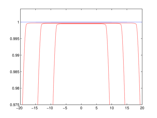
Figure 1: $J$ compactly supported

In Figure 1 we show convergence of $u_{R}$ to $u=1$. We observe that $u_{R}$ increases as $R$ increases (the values of $R$ are $R=10,15,20$).

6.2 Gaussian example

Consider the case

$$J(y)=\frac{1}{\sqrt{2\pi}}\mathrm{e}^{-y^{2}/2}.$$

Using the same ideas as in Section 4 we compute

$$H(p) = \frac{1}{\sqrt{2\pi}}\int_{\mathbb{R}}\mathrm{e}^{\,py-y^{2}/2}\,\mathrm{d}y-1$$

$$= \frac{1}{\sqrt{2\pi}}\int_{\mathbb{R}}\mathrm{e}^{-(p-y)^{2}/2}\cdot\mathrm{e}^{\,p^{2}/2}\,\mathrm{d}y-1$$

$$= \mathrm{e}^{\,p^{2}/2}-1.$$

Now, $D_{p}H(p)=p\mathrm{e}^{\,p^{2}/2}$ and $L(q)$ is obtained for $q=p\mathrm{e}^{\,p^{2}/2}$. For $q\to\infty$, we have $\ln q\sim\ln p+p^{2}/2\sim p^{2}/2$, thus $p\sim 2(\ln q)^{1/2}$ so that

$$L(q)\sim 2q(\ln q)^{1/2}\,.$$

In the picture on the left of Figure 2 we show again convergence for different values of $R$ ($R=10,15,20$). The picture on the right represents for $x$ and $t$ fixed the convergence of this point to the exact solution.

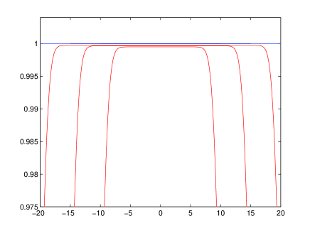
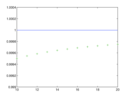
Figure 2: $J$ gaussian, $R=10,15,20$

6.3 Critical exponential decay

Finally we consider the case of a nucleus with critical exponential decay,

$$J=\frac{1}{2}\mathrm{e}^{-|y|}.$$

As we mentioned before, this case is not covered by the results of Section 3, but it shall illustrate how convergence works for a general case:

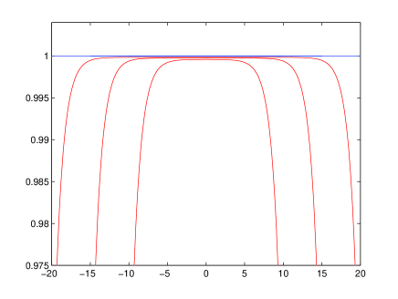
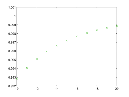
Figure 3: $J$ critical exponential decay, $R=10,15,20$

The picture on the right shows convergence of a point that moves with $R$; ı.e. we take a point of the form $(\theta R,t)$ with $t=0.1$ fixed and $\theta=0.8$.

References

• [1] G. Barles, Ch. Daher, M. Romano, Convergence of numerical schemes for parabolic equations arising in finance theory, Math. Models Methods Appl. Sci. 5 (1995), no. 1, 125–143.
• [2] G. Barles, E. Chasseigne & C. Imbert, Dirichlet boundary conditions for second order elliptic non-linear integro-differential equations, Indiana Univ. Math. J. 57 (2008), no. 1, 213–246.
• [3] G. Barles, C. Imbert, Second-order elliptic integro-differential equations: viscosity solutions’ theory revisited, Ann. Inst. H. Poincar Anal. Non Lin aire 25 (2008), no. 3, 567–585.
• [4] E. Chasseigne, M. Chaves, J.D. Rossi, Asymptotic behavior for nonlocal diffusion equations, J. Math. Pures Appl. (9) 86 (2006), no. 3, 271–291.
• [5] E. Chasseigne, The Dirichlet problem for some nonlocal diffusion equations, Differential Integral Equations. 20 (2007), no. 12, 1389–1404.
• [6] M.G. Crandall, P.-L Lions, Viscosity solutions of Hamilton-Jacobi equations. Trans. Amer. Math. Soc.277 (1983), no. 1, 1–42.
• [7] F. den Hollander, Large deviations, Fields Institute Monographs, 14. American Mathematical Society, Providence, RI (2000).
• [8] P.-L. Lions, Generalized solutions of Hamilton-Jacobi equations, Research Notes in Mathematics, 69. Pitman (Advanced Publishing Program), Boston, Mass.-London, (1982).
• [9] R.T. Rockafellar, Convex analysis. Princeton Mathematical Series, No. 28 Princeton University Press, Princeton, N.J. (1970).