GRAVITON, GHOST AND INSTANTON CONDENSATION
ON HORIZON SCALE OF UNIVERSE. DARK ENERGY AS
MACROSCOPIC EFFECT OF QUANTUM GRAVITY

Abstract

We show that cosmological acceleration (Dark Energy effect) falls into to a special class of quantum phenomena that occur on a macroscopic scale. Dark Energy is the third macroscopic quantum effect, the first after the discovery of superfluidity and superconductivity. Dark Energy is a phenomenon of quantum gravity on the scale of the Universe as a whole at any stage of its evolution, including the contemporary Universe. The effect is a direct consequence of the zero rest mass of gravitons, conformal non-invariance of the graviton field, and one-loop finiteness of quantum gravity, i.e. it is a direct consequence of first principles only. Therefore, no hypothetical fields or ”new physics” are needed to explain the Dark Energy effect. This macroscopic effect of one–loop quantum gravity takes place in the empty isotropic non–stationary Universe as well as in such a Universe filled by a non–relativistic matter or/and radiation. The effect is due to graviton–ghost condensates arising from the interference of quantum coherent states. Each of coherent states is a state of gravitons and ghosts of a wavelength of the order of the horizon scale and of different occupation numbers. The state vector of the Universe is a coherent superposition of vectors of different occupation numbers. One–loop approximation of quantum gravity is believed to be applicable to the contemporary Universe because of its remoteness from the Planck epoch. To substantiate the reliability of macroscopic quantum effects, the formalism of one–loop quantum gravity is discussed in detail. The theory is constructed as follows: Faddeev – Popov – De Witt gauged path integral $\longrightarrow$ factorization of classical and quantum variables, allowing the existence of a self–consistent system of equations for gravitons, ghosts and macroscopic geometry $\longrightarrow$ transition to the one–loop approximation, taking into account that contributions of ghost fields to observables cannot be eliminated in any way $\longrightarrow$ choice of ghost sector, satisfying the condition of one–loop finiteness of the theory off the mass shell. The Bogolyubov–Born–Green–Kirckwood–Yvon (BBGKY) chain for the spectral function of gravitons renormalized by ghosts is used to build a self–consistent theory of gravitons in the isotropic Universe. It is the first use of this technique in quantum gravity calculations. We found three exact solutions of the equations, consisting of BBGKY chain and macroscopic Einstein’s equations. It was found that these solutions describe virtual graviton and ghost condensates as well as condensates of instanton fluctuations. All exact solutions, originally found by the BBGKY formalism, are reproduced at the level of exact solutions for field operators and state vectors. It was found that exact solutions correspond to various condensates with different graviton–ghost compositions. Each exact solution corresponds to a certain phase state of graviton–ghost substratum. Quantum–gravity phase transitions are introduced. In the formalism of the BBGKY chain, the generalized self–consistent theory of gravitons is presented, taking into account the contribution of non–relativistic matter in the formation of a common self–consistent gravitational field. In the framework of this theory, it is shown that the era of non–relativistic matter dominance must be replaced by an era of dominance of graviton–ghost condensate. Pre–asymptotic state of Dark Energy is a condensate of virtual gravitons and ghosts with a constant conformal wavelength. The asymptotic state predicted by the theory is a self–polarized graviton–ghost condensate of constant physical wavelength in the De Sitter space. The Dark Energy phenomenon of such a nature is presented in the form of $\Lambda$GCDM model that interpolates the exact solutions of equations of one–loop quantum gravity. The proposed theory is compared with existing observational data on Dark Energy extracted from the Hubble diagram for supernovae SNIa. We show that $\Lambda$GCDM model has advantages over $\Lambda$CDM model if criteria for the statistical probability are in use. Result of processing of observational data suggests that the graviton–ghost condensate is an adequate variable component of Dark Energy. We show that its role was significant during the era of large–scale structure formation in the Universe.

I  Introduction

Macroscopic quantum effects are quantum phenomena that occur on a macroscopic scale. To date, there are two known macroscopic quantum effects: superfluidity at the scale of liquid helium vessel and superconductivity at the scale of superconducting circuits of electrical current. These effects have been thoroughly studied experimentally and theoretically understood. A key role in these effects is played by coherent quantum condensates of micro-objects with the De Broglie wavelength of the order of macroscopic size of the system. The third macroscopic quantum effect under discussion in this paper is condensation of gravitons and ghosts in the self–consistent field of the expanding Universe. Hypotheses on the possibility of graviton condensate formation in the Universe proposed by Hu 01 and Antoniadis–Mazur–Mottola 02 in a general form. A description of these effects by an adequate mathematical formalism is the problem at the present time.

We show that condensation of gravitons and ghosts is a consequence of quantum interference of states forming the coherent superposition. In this superposition, quantum fields have a certain wavelength, and with different amplitudes of probability they are in states corresponding to different occupation numbers of gravitons and ghosts. Intrinsic properties of the theory automatically lead to a characteristic wavelength of gravitons and ghosts in the condensate. This wavelength is always of the order of a distance to the horizon of events.

In this fact, a common feature of macroscopic quantum effects is manifested: such effects are always formed by quantum micro–objects, whose wavelengths are of the order of macroscopic values. With this in mind, we can say that macroscopic quantum gravity effects exist across the Universe as a whole. The results of this work suggest that the existence of the graviton–ghost condensate is directly responsible for the Dark Energy effect, i.e. for the observational data of the acceleration of the expansion of the Universe 03 ; 04 . Most significantly, a graviton–ghost condensate formation is direct consequence of the first principles of the theory of gravity and quantum field theory, so that no hypothetical fields are needed to explain the Dark Energy effect.

Quantum theory of gravity is a non–renormalized theory and for this reason it is impossible to calculate effects with an arbitrary accuracy in any order of the theory of perturbations. The program combining gravity with other physical interactions within the framework of supergravity or superstrings theory assumes the ultimate formulation of the theory containing no divergences. Today we do not have such a theory; nevertheless, we can hope to obtain physically meaningful results. Here are the reasons for this assumption.

First, in all discussed options for the future theory, Einstein’s theory of gravity is contained as a low energy limit. Second, from all physical fields, which will appear in a future theory (according to present understanding), only the quantum component of gravitational field (graviton field) has a unique combination of zero rest mass and conformal non–invariance properties. Third, physically meaningful effects of quantum gravity can be identified and quantified in one–loop approximation. Fourth, as was been shown by t’Hooft and Veltman 3 , the one–loop quantum gravity with ghost sector and without fields of matter is finite. For the property of one–loop finiteness, proven in 3 on the graviton mass shell, we add the following key assertion. All one–loop calculations in quantum gravity must be done in such a way that the feature of one–loop finiteness (lack of divergences in terms of observables) must automatically be implemented not only on the graviton mass shell but also outside it.

Let us emphasize the following important fact. Because of conformal non–invariance and zero rest mass of gravitons, no conditions exist in the Universe to place gravitons on the mass shell precisely. Therefore, in the absence of one–loop finiteness, divergences arise in observables. To eliminate them, the Lagrangian of Einstein’s theory must be modified, by amending the definition of gravitons. In other words, in the absence of one–loop finiteness, gravitons generate divergences, contrary to their own definition. Such a situation does not make any sense, so the one–loop finiteness off the mass shell is a prerequisite for internal consistency of the theory.

These four conditions provide for the reliability of theory predictions. Indeed, the existence of quantum component of the gravitational field leaves no doubt. Zero rest mass of this component means no threshold for quantum processes of graviton vacuum polarization and graviton creation by external or self–consistent macroscopic gravitational field. The combination of zero rest mass and conformal non–invariance of graviton field leads to the fact that these processes are occurring even in the isotropic Universe at any stage of its evolution, including the contemporary Universe. Vacuum polarization and particle creation belong to effects predicted by the theory already in one–loop approximation. In this approximation, calculations of quantum gravitational processes involving gravitons are not accompanied by the emergence of divergences. Thus, the one–loop finiteness of quantum gravity allows uniquely describe mathematically graviton contributions to the macroscopic observables. Other one–loop effects in the isotropic Universe are suppressed either because of conformal invariance of non–gravitational quantum fields, or (in the modern Universe) by non–zero rest mass particles, forming effective thresholds for quantum gravitational processes in the macroscopic self–consistent field.

Effects of vacuum polarization and particle creation in the sector of matter fields of $J=0,\ 1/2,\ 1$ spin were well studied in the 1970’s by many authors (see 52 and references therein). The theory of classic gravitational waves in the isotropic Universe was formulated by Lifshitz in 1946 13 . Grishchuk 40 considered a number of cosmological applications of this theory that are result of conformal non–invariance of gravitational waves. Isaacson 41 has formulated the task of self–consistent description of gravitational waves and background geometry. The model of Universe consisting of short gravitational waves was described for the first time in 20 . The energy–momentum tensor of classic gravitational waves of super long wavelengths was constructed in 42 ; 43 . The canonic quantization of gravitational field was done in 11 ; 44 ; HuParker1977 . The local speed of creation of shortwave gravitons was calculated in 45 . In all papers listed above, the ghost sector of graviton theory was not taken into account. One–loop quantum gravity in the form of the theory of gravitons defined on the background spacetime was described by De Witt 7 . Calculating methods of this theory were discussed by Hawking 37 . For the first time, the approach based on the fact that the ghost sector of graviton theory is determined by the condition of one–loop finiteness off the mass shell is presented in the present paper.

One–loop finiteness provides the simplicity and elegance of a mathematical theory that allows, in turn, discovering a number of new approximate and exact solutions of its equations. This paper is focused on three exact solutions corresponding to three different quantum states of graviton–ghost subsystem in the space of the non–stationary isotropic Universe with self–consistent geometry. The first of these solutions describes a coherent condensate of virtual gravitons and ghosts; the second solution describes a coherent condensate of instanton fluctuations. The third solution describes the self–polarized condensate in the De Sitter space. This solution allows interpretation in terms of virtual particles as well as in terms of instanton fluctuations. All three solutions are directly related to the physical nature of Dark Energy.

The principal nature of macroscopic quantum gravity effects, the need for strict proof of their inevitability and reliability impose stringent requirements for constructing a mathematical algorithm of the theory. In our view, existing versions of the theory of gravitons in macroscopic spacetime with self–consistent geometry do not meet these requirements. In this connection, note the following fact. Because of conformal non–invariance, the trace of the graviton energy–momentum tensor is not zero simply by definition of graviton field. Naturally, the information on macroscopic quantum effects (that are the subject of study in this paper) is contained in this trace. After the first publication of preliminary results of our research MUV we feel that a number of problems under discussion needs a much more detail description. Due to some superficial similarities, effects of graviton and ghost condensation in the De Sitter space are perceived sometime as another method of description of conformal anomalies, which are calculated by a traditional method of regularization and renormalization. (Calculations of such anomalies see in, e.g., 48 ; 49 ; 50 ; 51 ; TW ; MV .) We would like to emphasize that such analogies have neither physical nor mathematical basis. Conformal anomalies describe the effect of reconstruction of the spectrum of zero oscillations of quantum fields. Their contributions to the energy–momentum tensor are independent of state vector of the quantum field. They are parameterized by numerical coefficients of the order of unity that are factors of quadratic form of the curvature. Conformal anomalies that are microscopic quantum effects are able to contribute to the macroscopic evolution of the Universe only if its parameters are close to Planck ones. In contrast, the graviton and ghost condensation is a macroscopic quantum effect in the contemporary Universe. It is quantitatively described by macroscopic parameters that govern the structure of a state vector. These parameters are averaged numbers of quanta in coherent superpositions. Note also that in all papers known to us, calculations of anomalies were conducted in the framework of models with no one–loop finiteness off the graviton and ghost mass shell. It is shown in Appendices XII.1, XII.2 that such models are internally inconsistent. The rigorous theory of one–loop quantum gravity presented here shows that the effect of conformal anomalies on gravitons must be zero (see Appendix XII.3). In the empty Universe where the only gravitons exist, the De Sitter space can be formed by only a graviton–ghost condensate.

Sections II and III are devoted to the derivation of the equations of the theory with a discussion of all the mathematical details. In Section II, we start with exact quantum theory of gravity, presented in terms of path integral of Faddeev–Popov 5 and De Witt 4 . Key ideas of this Section are the following. (i) The necessity to gauge the full metric (before its separation into the background and fluctuations) and the inevitability of appearance of a ghost sector in the exact path integral and operator Einstein’s equations (Sections II.1 and II.2); (ii) The principal necessity to use normal coordinates (exponential parameterization) in a mathematically rigorous procedure for the separation of classical and quantum variables is discussed in Sections II.3 and II.4; (iii) The derivation of differential identities, providing the consistency of classical and quantum equations performed jointly in any order of the theory of perturbations is given Section II.5. Rigorously derived equations of gauged one–loop quantum gravity are presented in Section II.6.

The status of properties of ghost sector generated by gauge is crucial to properly assess the structure of the theory and its physical content. Let us immediately emphasize that the standard presentation on the ghost status in the theory of $S$–matrix can not be exported to the theory of gravitons in the macroscopic spacetime with self–consistent geometry. Two internal mathematical properties of the quantum theory of gravity make such export fundamentally impossible. First, there are no gauges that completely eliminate the diffeomorphism group degeneracy in the theory of gravity. This means that among the objects of the quantum theory of fields inevitably arise ghosts interacting with macroscopic gravity. Secondly, gravitons and ghosts cannot be in principle situated precisely on the mass shell because of their conformal non–invariance and zero rest mass. This is because there are no asymptotic states, in which interaction of quantum fields with macroscopic gravity could be neglected. Restructuring of vacuum graviton and ghost modes with a wavelength of the order of the distance to the horizon of events takes place at all stages of cosmological evolution, including the contemporary Universe. Ghost trivial vacuum, understood as the quantum state with zero occupation numbers for all modes, simply is absent from physically realizable states. Therefore, direct participation of ghosts in the formation of macroscopic observables is inevitable.

Section III is devoted to general discussion of equations of the theory of gravitons in the isotropic Universe. It focuses on three issues: (i) The gauge invariant procedure for eliminating gauge non–invariant modes by conditions imposed on the state vector (Section III.1); (ii) Construction of the state vector of a general form as a product of normalized superpositions (Section III.3); (iii) The allocation of class of legitimate gauges that are invariant with respect to transformations of the symmetry group of the background spacetime while providing the one–loop finiteness of macroscopic observables (Sections III.4 and III.5). The main conclusion is that the quantum ghost fields are inevitable and unavoidable components of the quantum gravitational field. As noted above, one–loop finiteness is seen by us as a universal property of quantum gravity, which extends off the mass shell. The requirement of compensation of divergences in terms of macroscopic observables, resulting from one–loop finiteness, uniquely captures the dynamic properties of quantum ghost fields in the isotropic Universe.

The treatment set out in Sections II and III, in essence, is a sequence of transformations of equations defined by original gauged path integral. Basically, these transformations are of mathematical identity nature. There are only three elements of the theory, missing in the original integral:

(i) The hypothesis of the existence of classical spacetime with the deterministic but self–consistent geometry;

(ii) A transition to the one–loop approximation in the self–consistent system of classical and quantum equations;

(iii) A class of gauges that automatically provides the one–loop finiteness of self–consistent theory of gravitons in the isotropic Universe.

Conceptually discussing of the first two additional elements was not necessary. Their introduction to the formalism is to the factorization of measure of path integral and expansion of equations of the theory in a series of powers of the graviton field. The existence of appropriate correct mathematical procedures is not in doubt. Agreement on choosing of a gauge is also mathematically consistent. Moreover, a gauge is necessary for the strict definition of path integral as a mathematical object.

The existence of class of gauges, automatically providing one–loop finiteness off the mass shell is itself a nontrivial property of the theory. The assertion that only such gauges can be used in the self–consistent theory of gravitons in the isotropic Universe is actually a condition for the internal consistency of the theory. In Appendix XII.2, we present the formal proof that an alternative formulation of the theory (with no one–loop finiteness) does not exist.

From the requirement of the one–loop finiteness it follows that the quantum component of the gravitational field is of a heterogeneous graviton–ghost structure. In further Sections of work, it appears that this new element of the theory prejudge its physical content.

Sections IV.1 and IV.2 contain approximate solutions to obtain quantum ensembles of short and long gravitational waves. In Section IV.3 it is shown that approximate solutions obtained can be used to construct scenarios for the evolution of the early Universe. In one such scenario, the Universe is filled with ultra–relativistic gas of short–wave gravitons and with a condensate of super–long wavelengths, which is dominated by ghosts. The evolution of this Universe is oscillating in nature.

At the heart of cosmological applications of one–loop quantum gravity is the Bogolyubov–Born–Green–Kirckwood–Yvon (BBGKY) chain (or hierarchy) for the spectral function of gravitons, renormalized by ghosts. We present the first use of this technique in quantum gravity calculations. Each equation of the BBGKY chain connects the expressions for neighboring moments of the spectral function. In Section V.1 the BBGKY chain is derived by identical mathematical procedures from graviton and ghost operator equations. Among these procedures is averaging of bilinear forms of field operators over the state vector of the general form, whose mathematical structure is given in Section III.3. The need to work with state vectors of the general form is dictated by the instability of the trivial graviton–ghost vacuum (Section III.6). Evaluation of mathematical correctness of procedures for BBGKY structure is entirely a question of the existence of moments of the spectral function as mathematical objects. A positive answer to this question is guaranteed by one–loop finiteness (Section III.4). The set of moments of the spectral function contains information on the dynamics of operators as well as on the properties of the quantum state over which the averaging is done. The set of solutions of BBGKY chain contains all possible self–consistent solutions of operator equation, averaged over all possible quantum ensembles.

A nontrivial fact is that in the one–loop quantum gravity BBGKY chain can formally be introduced at an axiomatic level. Theory of gravitons provided by BBGKY chain, conceptually and mathematically corresponds to the axiomatic quantum field theory in the Wightman formulation (see Chapter 8 in the monograph 6 ). Here, as in Wightman, the full information on the quantum field is contained in an infinite sequence of averaged correlation functions. Definitions of these functions clearly relate to the symmetry properties of manifold on one this field is defined. Once the BBGKY chain is set up, the existence of finite solutions for the observables is provided by inherent mathematical properties of equations of the chain. This means that the phenomenology of BBGKY chain is more general than field operators, state vectors and graviton–ghost compensation of divergences that were used in its derivation.

Exact solutions of the equations, consisting of BBGKY chain and macroscopic Einstein’s equations are obtained in Sections V.2 and V.3. Two solutions given in V.2, describe heterogeneous graviton–ghost condensates, consisting of three subsystems. Two of these are condensates of spatially homogeneous modes with the equations of state $p=-\varepsilon/3$ and $p=\varepsilon$. The third subsystem is a condensate of quasi–resonant modes with a constant conformal wavelength corresponding to the variable physical wavelength of the order of the distance to the horizon of events. The equations of state of condensates of quasi–resonant modes differ from $p\sim-\varepsilon/3$ by logarithmic terms, through which the first solution is $p\gtrsim-\varepsilon/3$, while the second is $p\lesssim-\varepsilon/3$. Furthermore, the solutions differ by the sign of the energy density of condensates of spatially homogenous modes. The third solution describes a homogeneous condensate of quasi–resonant modes with a constant physical wavelength. The equation of state of this condensate is $p=-\varepsilon$ and its self–consistent geometry is the De Sitter space. The three solutions are interpreted as three different phase states of graviton–ghost system. The problem of quantum–gravity phase transitions is discussed in SectionV.4.

Solutions obtained in Section V in terms of moments of the spectral function, are reproduced in Sections VI and VII at the level of dynamics of operators and state vectors. A microscopic theory provides details to clarify the structure of graviton–ghost condensates and clearly demonstrates the effects of quantum interference of coherent states. In Section VI.1 it is shown that the condensate of quasi–resonant modes with the equation of state $p\gtrsim-\varepsilon/3$ consists of virtual gravitons and ghosts. In Section VI.2 a similar interpretation is proposed for the condensate in the De Sitter space, but it became necessary to extend the mathematical definition of the moments of the spectral function.

New properties of the theory, whose existence was not anticipated in advance, are studied in Section VII. In Section VII.1 we find that the self–consistent theory of gravitons and ghosts is invariant with respect to the Wick turn. In this Section we also construct the formalism of quantum theory in the imaginary time and discuss the physical interpretation of this theory. The subjects of the study are correlated fluctuations arising in the process of tunnelling between degenerate states of graviton–ghost systems, divided by classically impenetrable barriers. The level of these fluctuations is evaluated by instanton solutions (as in Quantum Chromodynamics). In Section VII.2 it is shown that the condensate of quasi–resonant modes with the equation of state $p\lesssim-\varepsilon/3$ is of purely instanton nature. In Section VII.3 the instanton condensate theory is formulated for the De Sitter space.

Potential use of the results obtained to construct scenarios of cosmological evolution was briefly discussed in Sections IV — VII to obtain approximate and exact solutions. A main application of the theory of macroscopic effects of quantum gravity is to explain the physics of Dark Energy. As a carrier of Dark Energy, quantum gravity offers graviton–ghost condensate of quasi–resonant modes. In Section VIII the theory of gravitons and ghosts is formulated in a self–consistent field, in the formation of which heavy particles (baryons and particles of Dark Matter (neutralino as a example)) are involved. In Section VIII.1 it is shown that the cosmological solution describing the evolution of the scale factor, non–relativistic matter and graviton–ghost subsystem, automatically satisfies the chain integral identities contained in the equations of this theory. From these identities it follows that the stage of the Universe evolution, which is dominated by non–relativistic matter, must inevitably be replaced by a stage at which substantive contribution to the energy density of the cosmological substratum will produce graviton–ghost condensate of quasi–resonant modes of a constant conformal wavelength. This stage of the Universe evolution we consider as the pre–asymptotic one. Conversion of pre–asymptotic condensate to a condensate of constant physical wavelength occurs in the process of quantum–gravity phase transition.

In Section VIII.2 the exact solutions of equations of the one–loop quantum gravity are used to construct model of Dark Energy, intended for interpretation of experimental data. The model is based on simple interpolation formulae, describing the energy density and pressure of graviton–ghost condensates at various stages of cosmological evolution. For the cosmological model based on the physical considerations presented here, we suggest the abbreviation ”$\Lambda$GCDM model.”  Here ”CDM” means Cold Dark Matter; ”G” means a graviton–ghost condensate in the role of Dark Energy; symbol $\Lambda$ indicates an asymptotic state of the Universe in which the energy density of cosmological substratum goes to a constant value. The following cosmological Einstein equations correspond to the $\Lambda$GCDM model

$$\begin{array}[]{c}\displaystyle 3H^{2}=\varkappa\left(\varepsilon_{g}+\frac{M}{a^{3}}\right),\qquad 6Q=-\varkappa\left(\varepsilon_{g}+3p_{g}+\frac{M}{a^{3}}\right)\ ,\end{array}$$ (I.1)

where

$$\begin{array}[]{c}\displaystyle\varepsilon_{g}=\Lambda_{\infty}+\frac{C_{g}}{a^{2}}\ln\frac{a_{0}}{a}\ ,\qquad p_{g}=-\Lambda_{\infty}-\frac{C_{g}}{3a^{2}}\ln\frac{a_{0}}{ea}\ .\end{array}$$ (I.2)

are energy density and pressure of graviton–ghost medium; $M/a^{3}$ is the density of non–relativistic matter; $H=\dot{a}/a$ is Hubble function; $Q=\ddot{a}/a$ is acceleration of the Universe expansion. The symbol $\Lambda_{\infty}$ indicates the asymptotic value of total energy density of graviton–ghost condensate and equilibrium vacuum of non–gravitational physical fields. Note that $\Lambda_{\infty}\neq 0$, even if the non–gravitational vacuum energy (”standard” Einstein’s cosmological constant) vanishes by some compensation mechanisms of the type of supersymmetry.

As can be seen from (I.2), the theory of graviton–ghost condensates in an extremely simplified version predicted by a three–parameter model of Dark Energy. A quantitative comparison of theory with the observational data is conducted in Section IX. Section IX.1 devoted to a brief review of the physics of Dark Energy problems. Synopsis of observational data on supernovae SNIa is given in Section IX.2. Our focus is on the choice between $\Lambda$CDM and $\Lambda$GCDM models based on general principles of fundamental physics without involving hypothetical elements. In Section IX.3 a comparative analysis of the results of processing the Hubble diagram for SNIa by formulas for both models is conducted. Here we show that the $\Lambda$GCDM model not only explains quantitatively the effect of Dark Energy, but also reproduces a number of specific details of observational data.

The results and problems of the theory are briefly discussed in the Conclusion (Section X). Appendix XI is devoted to the cosmological constant problem within the framework of its interpretation as the energy density of equilibrium vacuum of non–gravitational physical fields. An internal inconsistency of the theory which lacks one–loop finiteness off the mass shell is proved in Appendices XII.1,XII.2. In XII.3, it is shown by the method of dimensional transmutation that the one–loop self–consistent theory of gravitons and ghosts is not only finite but is also free of anomalies.

A system of units is used, in which the speed of light is $c=1$, Planck constant is $\hbar=197.327$ MeV$\cdot$fm; Einstein’s gravity constant is $\varkappa\equiv 8\pi G=8\pi\cdot 1.324\cdot 10^{-42}$ MeV${}^{-1}\cdot$fm.

II Basic Equations

According to De Witt 7 , one of formulations of one–loop quantum gravity (with no fields of matter) is reduced to the zero rest mass quantum field theory with spin $J=2$, defined for the background spacetime with classic metric. The graviton dynamics is defined by the interaction between quantum field and classic gravity, and the background space geometry, in turn, is formed by the energy–momentum tensor (EMT) of gravitons.

In the current Section we describe how to get the self–consistent system of equations, consisting of quantum operator equations for gravitons and ghosts and classic $C$–number Einstein equations for macroscopic metrics with averaged EMT of gravitons and ghosts on the right hand side. The theory is formulated without any constrains on the graviton wavelength that allows the use of the theory for the description of quantum gravity effects at the long wavelength region of the specter. The equations of the theory (except the gauge condition) are represented in 4D form which is general covariant with respect to the transformation of the macroscopic metric.

The mathematically consistent system of 4D quantum and classic equations with no restrictions with respect to graviton wavelengths is obtained by a regular method for the first time. The case of a gauged path integral with ghost sector is seen as a source object of the theory. Important elements of the method are exponential parameterization of the operator of the density of the contravariant metric; factorization of path integral measure; consequent integration over quantum and classic components of the gravitational field. Mutual compliance of quantum and classic equations, expressed in terms of fulfilling of the conservation of averaged EMT at the operator equations of motion is provided by the virtue of the theory construction method.

II.1 Path Integral and Faddeev–Popov Ghosts

Formally, the exact scheme of quantum gravity is based on the amplitude of transition, represented by path integral 4 ; 5 :

$$\begin{array}[]{c}\displaystyle\langle\mbox{\rm out}|\mbox{\rm in}\rangle=\int\exp\left(\frac{i}{\hbar}\int(L_{grav}+L_{\Lambda})d^{4}x\right)\left(\mbox{\rm det}\,\hat{M}^{i}_{\;k}\right)\prod_{x}\left(\prod_{i}\delta(\hat{A}_{k}\sqrt{-\hat{g}}\hat{g}^{ik}-B^{i})\right)d\hat{\mu}=\\[14.22636pt] \displaystyle=\int\exp\left(\frac{i}{\hbar}\int(L_{grav}+L_{\Lambda}+L_{ghost})d^{4}x\right)\prod_{x}\left(\prod_{i}\delta(\hat{A}_{k}\sqrt{-\hat{g}}\hat{g}^{ik}-B^{i})\right)d\hat{\mu}d\mu_{\theta}\ ,\end{array}$$ (II.1)

where

$$L_{grav}+L_{\Lambda}=-\frac{1}{2\varkappa}\sqrt{-\hat{g}}\hat{g}^{ik}\hat{R}_{ik}-\sqrt{-\hat{g}}\Lambda$$

is the density of gravitational Lagrangian, with cosmological constant included; $L_{ghost}$ is the density of ghost Lagrangian, explicit form of which is defined by localization of $\mbox{\rm det}\,\hat{M}^{i}_{\;k}$; $\hat{A}_{k}$ is gauge operator, $B^{i}(x)$ is the given field; $\hat{M}^{i}_{\;k}$ is an operator of equation for infinitesimal parameters of transformations for the residual degeneracy $\eta^{i}=\delta x^{i}$;

$$d\hat{\mu}=\prod_{x}\left\{(-\hat{g})^{5/2}\prod_{i\leqslant k}d\hat{g}^{ik}\right\}$$ (II.2)

is the gauge invariant measure of path integration over gravitational variables; $d\mu_{\theta}$ is the measure of integration over ghost variables. Operator $\hat{M}^{i}_{\;k}$ is of standard definition:

$$\hat{M}^{i}_{\;k}\eta^{k}\equiv\hat{A}_{k}(\delta\sqrt{-\hat{g}}\hat{g}^{ik})=0,$$ (II.3)

where

$$\delta\sqrt{-\hat{g}}\hat{g}^{ik}=-\partial_{l}(\sqrt{-\hat{g}}\hat{g}^{ik}\eta^{l})+\sqrt{-\hat{g}}\hat{g}^{il}\partial_{l}\eta^{k}+\sqrt{-\hat{g}}\hat{g}^{kl}\partial_{l}\eta^{i}$$ (II.4)

is variation of metrics under the action of infinitesimal transformations of the group of diffeomorphisms. According to (II.1), the allowed gauges are constrained by the condition of existence of the inverse operator $(\hat{M}^{i}_{\;k})^{-1}$.

The equation (II.1) explicitly manifests the fact that the source path integral is defined as a mathematical object only after the gauge has been imposed. In the theory of gravity, there are no gauges completely eliminating the degeneracy with respect to the transformations (II.4). Therefore, the sector of nontrivial ghost fields, interacting with gravity, is necessarily present in the path integral. This aspect of the quantum gravity is important for understanding of its mathematical structure, which is fixed before any approximations are introduced. By that reason, in this Section we discuss the equations of the theory, by explicitly defining the concrete gauge.

In cosmological applications of the quantum gravity it is convenient to use synchronous gauges of type:

$$\sqrt{-\hat{g}}\hat{g}^{00}=\sqrt{\bar{\gamma}}\ ,\qquad\sqrt{-\hat{g}}\hat{g}^{0\alpha}=0\ .$$ (II.5)

For that gauge

$$\hat{A}_{k}=(1,\,0,\,0,\,0)\ ,\qquad B^{i}=(\sqrt{\bar{\gamma}},\,0,\,0,\,0),$$ (II.6)

where $\bar{\gamma}=\bar{\gamma}({\bf x})$ is the metric determinant of the basic 3D space of constant curvature (for the plane cosmological model $\bar{\gamma}=1$). More general approach to the choice of gauge used for cosmological problems is discussed in Section III.5.

The construction of the ghost sector, i.e. finding of the Lagrangian density $L_{ghost}$, is reduced to two operations. First, $\mbox{\rm det}\,\hat{M}^{i}_{\;k}$ is represented in the form, factorized over independent degrees of freedom for ghosts, and then the localization of the obtained expression is conducted. Substitution of (II.6) and (II.4) to (II.3) gives the following system of equations

$$-\partial_{\alpha}\sqrt{\bar{\gamma}}\eta^{\alpha}+\sqrt{\bar{\gamma}}\frac{\partial\eta^{0}}{\partial t}=0,\qquad\sqrt{-\hat{g}}\hat{g}^{\alpha\beta}\partial_{\beta}\eta^{0}+\frac{\partial\sqrt{\bar{\gamma}}\eta^{\alpha}}{\partial t}=0.$$ (II.7)

According to (II.7), with respect to variables $\eta^{0}$, $\sqrt{\bar{\gamma}}\eta^{\alpha}$ the operator–matrix $\hat{M}^{i}_{\;k}$ reads

$$\hat{M}^{i}_{\;k}=\begin{pmatrix}\displaystyle\sqrt{\bar{\gamma}}\frac{\partial}{\partial t}&\quad-\partial_{\alpha}\\[14.22636pt] \displaystyle\sqrt{-\hat{g}}\hat{g}^{\alpha\beta}\partial_{\beta}&\quad\displaystyle\delta_{\beta}^{\alpha}\frac{\partial}{\partial t}\end{pmatrix}$$ (II.8)

(Note matrix–operator is obtained in the form (II.8) without the substitution of transformation parameters if Leutwiller measure $d\hat{\mu}_{L}=\hat{g}\hat{g}^{00}d\hat{\mu}$ is used. The measure discussion see, e.g. 8 .) Functional determinant of matrix–operator $\mbox{\rm det}\,\hat{M}^{i}_{\;k}$ is represented in the form of the determinant of matrix $\hat{M}^{i}_{\;k}$, every element of which is a functional determinant of differential operator. As it is follows from (II.8),

$$\mbox{\rm det}\,\hat{M}^{i}_{\;k}=\left(\mbox{\rm det}\;\partial_{i}\sqrt{\hat{g}}\hat{g}^{ik}\partial_{k}\right)\times\left(\mbox{\rm det}\;\frac{\partial}{\partial t}\right)\times\left(\mbox{\rm det}\;\frac{\partial}{\partial t}\right).$$ (II.9)

One can see that the first multiplier in (II.9) is 4–invariant determinant of the operator of the zero rest mass Klein–Gordon–Fock equation, and two other multipliers do not depend on gravitational variables.

Localization of determinant (II.9) by representing it in a form of path integral over the ghost fields is a trivial operation. As it follows from (II.9), the class of synchronous gauges contains three dynamically independent ghost fields $\theta,\,\varphi,\,\chi$, two of each — $\varphi,\,\chi$ do not interact with gravity. For the obvious reason, the trivial ghosts $\varphi,\,\chi$ are excluded from the theory. The Lagrangian density of nontrivial ghosts coincides exactly with Lagrangian density of complex Klein–Gordon–Fock fields (taking into account the Grassman character of fields $\bar{\theta},\,\theta$):

$$L_{ghost}=-\frac{1}{4\varkappa}\sqrt{-\hat{g}}\hat{g}^{ik}\partial_{i}\bar{\theta}\cdot\partial_{k}\theta.$$ (II.10)

The normalization multiplier $-1/4\varkappa$ in (II.10) is chosen for the convenience. The integral measure over ghost fields has a simple form:

$$d\mu_{\theta}=\prod_{x}d\bar{\theta}d\theta\ .$$

The calculations above comply with both general requirements to the construction of ghost sector. First, path integration should be carried out only over the dynamically independent ghost fields. Second, in the ghost sector, it is necessary to extract and then to take into account only the nontrivial ghost fields, i.e. those interacting with gravity.

The extraction of dynamically independent nontrivial ghost fields can be done not only by factorization of functional determinant (as it made in (II.9)), but by means of researching the equations for the ghosts as well. It is well known 9 , that from the definition of $\mbox{\rm det}\,\hat{M}^{i}_{\;k}$ it follows that the ghost equations coincide with equations for parameters of infinitesimal transformations of residual degeneracy. Therefore, according to (II.3), we can immediately get $\hat{M}^{i}_{\;k}\theta^{k}=0$, where $\theta^{k}$ are the Grassman fields. For the gauge (II.5) with $B=1$ we get

$$-\partial_{\alpha}\sqrt{\bar{\gamma}}\theta^{\alpha}+\sqrt{\bar{\gamma}}\frac{\partial\theta^{0}}{\partial t}=0,$$ (II.11)

$$\sqrt{-\hat{g}}\hat{g}^{\alpha\beta}\partial_{\beta}\theta^{0}+\frac{\partial\sqrt{\bar{\gamma}}\theta^{\alpha}}{\partial t}=0.$$ (II.12)

From (II.12) it follows that those transversal components of vector $\theta^{\alpha}$ yield the equations $\partial\theta^{\alpha}_{\perp}/\partial t=0$, i.e. these degrees of freedom correspond to two trivial ghosts non–interacting with gravity. Note, that in (II.11) only the longitudinal component $\theta^{\alpha}_{\parallel}$ is present. Equation (II.12) has a status of equation connecting the longitudinal component $\theta^{\alpha}_{\parallel}$ and function $\theta^{0}$. It means that the longitudinal field $\theta^{\alpha}_{\parallel}$ is not dynamically independent. Equation for dynamically independent degrees of freedom $\theta^{0}$ is obtained as follows. First, the operator $\partial_{\alpha}$ is applied to the equation (II.12), next the result is substituted into time–differentiated equation (II.11). After the substitution, one gets Klein–Gordon–Fock equation,

$$\frac{\partial}{\partial t}\sqrt{\bar{\gamma}}\frac{\partial\theta}{\partial t}+\partial_{\alpha}\sqrt{-\hat{g}}\hat{g}^{\alpha\beta}\partial_{\beta}\theta=\partial_{i}\sqrt{-\hat{g}}\hat{g}^{ik}\partial_{k}\theta=0\ ,$$ (II.13)

where $\theta=\theta^{0}$. Reconstruction of the ghost Lagrangian (II.10) from dynamical equation (II.13) does not require an additional explanation.

Thus, the prove of wave properties of ghosts in the class of synchronous gauges is done by two methods with clear correlations between objects and operations used in these methods.

We will return to the discussion of gauges and ghosts in the Section III.5.

II.2 Einstein Operator Equations

Let us take into account the fact that the calculation of gauged path integral should be mathematically equivalent to the solution of dynamical operator equations in the Heisenberg representation. It is also clear that operator equations of quantum theory should have a definite relationship with Einstein equations. In the classic theory, it is possible to use any form of representation of Einstein equations, e.g.

$$\begin{array}[]{c}\displaystyle(-\hat{g})^{n}\left(\hat{g}^{il}\hat{g}^{km}\hat{R}_{lm}-\frac{1}{2}\hat{g}^{ik}\hat{g}^{lm}\hat{R}_{lm}-\hat{g}^{ik}\varkappa\Lambda\right)=0\ ,\qquad(a)\\[8.53581pt] \displaystyle(-\hat{g})^{n}\left(\hat{g}^{km}\hat{R}_{im}-\frac{1}{2}\delta_{i}^{k}\hat{g}^{lm}\hat{R}_{lm}-\delta_{i}^{k}\varkappa\Lambda\right)=0\ ,\qquad\qquad(b)\\[8.53581pt] \displaystyle(-\hat{g})^{n}\left(\hat{R}_{ik}-\frac{1}{2}\hat{g}_{ik}\hat{g}^{lm}\hat{R}_{lm}-\hat{g}^{ik}\varkappa\Lambda\right)=0\ ,\qquad\qquad\qquad(c)\end{array}$$ (II.14)

where, for example, $n=0,\;1/2,\;1$. Transition from one to another is reduced to the multiplication by metric tensor and its determinant, which are trivial operations in case when the metric is a $C$–number function. If the metric is an operator, then the analogous operations will, at least, change renormalization procedures of quantum non–polynomial theory. Thus, the question about the form of notation for Einstein’s operator equations has first–hand relation to the calculation procedure. Now we show that in the quantum theory one should use operator equations (II.14$b$) with $n=1/2$, supplemented by the energy–momentum pseudo–tensor of ghosts.

In the path integral formalism, the renormalization procedures are defined by the dependence of Lagrangian of interactions and the measure of integration of the field operator in terms of which the polynomial expansion of non–polynomial theory is defined 9 . The introduction of such an operator, i.e. the parameterization of the metric, is, generally speaking, not simple. Nevertheless, it is possible to find a special parameterization for which the algorithms of renormalization procedures are defined only by Lagrangian of interactions. Obviously, in such a parameterization the measure of integration should be trivial. It reads:

$$d\hat{\mu}=\prod_{x}\prod_{i\leqslant k}d\hat{\Psi}_{i}^{k}\ ,$$ (II.15)

where $\hat{\Psi}_{i}^{k}$ is a dynamic variable. The metric is expressed via this variable. It is shown in 9 that the trivialization of measure (II.15) takes place for the exponential parameterization that reads

$$\begin{array}[]{c}\displaystyle\sqrt{-\hat{g}}\hat{g}^{ik}=\sqrt{-\bar{g}}\bar{g}^{il}(\exp{\hat{\Psi}})_{l}^{k}=\sqrt{-\bar{g}}\bar{g}^{il}\left(\delta_{l}^{k}+\hat{\Psi}_{l}^{k}+\frac{1}{2}\hat{\Psi}_{l}^{m}\hat{\Psi}_{m}^{k}+\ldots\right)\ ,\end{array}$$ (II.16)

where $\bar{g}^{ik}$ is the defined metric of an auxiliary basic space. In that class of our interest, the metric is defined by the interval

$$d\bar{s}^{2}=dt^{2}-\bar{\gamma}_{\alpha\beta}dx^{\alpha}dx^{\beta}\ ,$$

where $\bar{\gamma}_{\alpha\beta}$ is the metric of 3D space with a constant curvature. (For the flat Universe $\bar{\gamma}_{\alpha\beta}$ is the Euclid metric.)

The exponential parameterization is singled out among all other parameterizations by the property that $\hat{\Psi}_{i}^{k}$ are the normal coordinates of gravitational fields 10 . In that respect, the gauge conditions (II.5) are identical to $\hat{\Psi}_{0}^{i}=0$. The fact that the ”gauged” coordinates are the normal coordinates, leads to a simple and elegant ghost sector (II.10). The status of $\hat{\Psi}_{i}^{k}$, as normal coordinates, is of principal value for the mathematical correctness while separating the classic and quantum variables (see Section II.4). Besides, in the framework of perturbation theory the normal coordinates allow to organize a calculation procedure, which is based on a simple classification of nonlinearity of quantum gravity field. It is important that this procedure is mathematically non–contradictive at every order of perturbation theory over amplitude of quantum fields (see Section II.5, II.6).

Operator Einstein equations that are mathematically equivalent to the path integral of a trivial measure are derived by the variation of gauged action by variables $\hat{\Psi}_{i}^{k}$. The principal point is that the gauged action necessarily includes the ghost sector because there are no gauges that are able to completely eliminate the degeneracy. According to (II.10), in the class of synchronous gauges we get

$$S=-\int d^{4}x\left\{\frac{1}{2\varkappa}\sqrt{-\hat{g}}\hat{g}^{ik}\left(\hat{R}_{ik}+\frac{1}{2}\partial_{i}\bar{\theta}\cdot\partial_{k}\theta\right)+\sqrt{-\hat{g}}\Lambda\right\}\ .$$ (II.17)

In accordance with definition (II.16), the variation is done by the rule

$$\delta\sqrt{-\hat{g}}\hat{g}^{ik}=\sqrt{-\hat{g}}\hat{g}^{il}\delta\hat{\Psi}_{l}^{k}\ .$$

Thus, from (II.17) it follows

$$\hat{\mathcal{G}}_{i}^{k}\equiv\sqrt{-\hat{g}}\hat{g}^{kl}\hat{R}_{il}-\varkappa\left(\sqrt{-\hat{g}}\hat{g}^{kl}\hat{T}^{(ghost)}_{il}-\frac{1}{2}\delta_{i}^{k}\sqrt{-\hat{g}}\hat{g}^{ml}\hat{T}^{(ghost)}_{ml}-\sqrt{-\hat{g}}\delta_{i}^{k}\Lambda\right)=0\ .$$ (II.18)

After subtraction of semi–contraction from (II.18) we obtain a mathematically equivalent equation

$$\begin{array}[]{c}\displaystyle\hat{\mathcal{E}}_{i}^{k}=\hat{\mathcal{G}}_{i}^{k}-\frac{1}{2}\delta_{i}^{k}\hat{\mathcal{G}}_{l}^{l}\equiv\\[14.22636pt] \displaystyle\sqrt{-\hat{g}}\hat{g}^{kl}\hat{R}_{il}-\frac{1}{2}\delta_{i}^{k}\sqrt{-\hat{g}}\hat{g}^{ml}\hat{R}_{ml}-\varkappa\left(\sqrt{-\hat{g}}\hat{g}^{kl}\hat{T}^{(ghost)}_{il}+\sqrt{-\hat{g}}\delta_{i}^{k}\Lambda\right)=0\ .\end{array}$$ (II.19)

In (II.18), (II.19) there is an object

$$\hat{T}^{(ghost)}_{ik}=-\frac{1}{4\varkappa}\left(\partial_{i}\bar{\theta}\cdot\partial_{k}\theta+\partial_{k}\bar{\theta}\cdot\partial_{i}\theta-\hat{g}_{ik}\hat{g}^{lm}\partial_{l}\bar{\theta}\cdot\partial_{m}\theta\right)\ ,$$ (II.20)

which has the status of the energy–momentum pseudo–tensor of ghosts.

In accordance with the general properties of Einstein’s theory, six spatial components of equations (II.18) are considered as quantum equations of motion:

$$\sqrt{-\hat{g}}\hat{g}^{\beta l}\hat{R}_{\alpha l}=\varkappa\left(\sqrt{-\hat{g}}\hat{g}^{\beta l}\hat{T}^{(ghost)}_{\alpha l}-\frac{1}{2}\delta_{\alpha}^{\beta}\sqrt{-\hat{g}}\hat{g}^{ml}\hat{T}^{(ghost)}_{ml}-\sqrt{-\hat{g}}\delta_{\alpha}^{\beta}\Lambda\right)\ .$$ (II.21)

(Everywhere in this work the Greek metric indexes stand for $\alpha,\ \beta=1,\ 2,\ 3$.) In the classic theory, equations of constraints $\hat{\mathcal{E}}_{0}^{0}=0$ and $\hat{\mathcal{E}}_{0}^{\alpha}=0$ are the first integrals of equations of motion (II.21). Therefore, in the quantum theory formulated in the Heisenberg representation four primary constraints from (II.19), have the status of the initial conditions for the Heisenberg state vector. They read:

$$\begin{array}[]{c}\displaystyle\left\{\sqrt{-\hat{g}}\hat{g}^{0l}\hat{R}_{0l}-\frac{1}{2}\sqrt{-\hat{g}}\hat{g}^{ml}\hat{R}_{ml}-\varkappa\left(\sqrt{-\hat{g}}\hat{g}^{0l}\hat{T}^{(ghost)}_{0l}+\sqrt{-\hat{g}}\Lambda\right)\right\}|\Psi\rangle=0\ ,\\[8.53581pt] \displaystyle\left\{\sqrt{-\hat{g}}\hat{g}^{\alpha l}\hat{R}_{0l}-\varkappa\sqrt{-\hat{g}}\hat{g}^{\alpha l}\hat{T}^{(ghost)}_{0l}\right\}|\Psi\rangle=0\ .\end{array}$$ (II.22)

If conditions (II.22) are valid from the start, then the internal properties of the theory must provide their validity at any subsequent moment of time. Four secondary relations, defined by the gauge non containing the higher order derivatives, also have the same status:

$$\left\{\hat{A}_{k}(\sqrt{-\hat{g}}\hat{g}^{ik})-B^{i}\right\}|\Psi\rangle=0\ .$$ (II.23)

The system of equations of quantum gravity is closed by the ghosts’ equations of motion, obtained by the variation of action (II.17) over ghost variables:

$$\begin{array}[]{c}\displaystyle\partial_{i}\sqrt{-\hat{g}}\hat{g}^{ik}\partial_{k}\theta=0\ ,\\[8.53581pt] \displaystyle\partial_{i}\sqrt{-\hat{g}}\hat{g}^{ik}\partial_{k}\bar{\theta}=0\ .\end{array}$$ (II.24)

Ghost fields $\bar{\theta}$ and $\theta$ are not defined by Grassman scalars, therefore $T^{(ghost)}_{ik}$ is not a tensor. Nevertheless, all mathematical properties of equations (II.24) and expressions (II.20) coincide with the respected properties of equations and EMT of complex scalar fields. This fact is of great importance when concrete calculations are done (see Section III).

II.3 Factorization of the Path Integral

Transition from the formally exact scheme (II.21) — (II.24)) to the semi–quantum theory of gravity can be done after some additional hypotheses are included in the theory. The physical content of these hypotheses consists of the assertion of existence of classical spacetime with metric $g_{ik}$, connectivity $\Gamma^{i}_{kl}$ and curvature $R_{ik}$. The first hypothesis is formulated at the level of operators. Assume that operator of metric $\hat{g}^{ik}$ is a functional of $C$–number function $g^{ik}$ and the quantum operator $\hat{\psi}_{i}^{k}$. The second hypothesis is related to the state vector. Each state vector that is involved in the scalar product $\langle\mbox{\rm out}|\mbox{\rm in}\rangle$, is represented in a factorized form $|\Psi\rangle=|\Phi\rangle|\psi\rangle$, where $|\psi\rangle$ are the vectors of quantum states of gravitons; $|\Phi\rangle$ are the vectors of quasi–classic states of macroscopic metric. In the framework of these hypotheses the transitional amplitude is reduced to the product of amplitudes:

$$\langle\mbox{\rm out}|\mbox{\rm in}\rangle=\langle\Phi_{out}|\Phi_{in}\rangle\langle\psi_{out}|\psi_{in}\rangle\ .$$ (II.25)

Thus, the physical assumption about existence of classic spacetime formally (mathematically) means that the path integral must be calculated first by exact integration over quantum variables, and then by approximate integration over the classic metric.

Mathematical definition of classic and quantum variables with subsequent integrations are possible only after the trivialization and factorization of integral measure are done. As already noted, trivial measure (II.15) takes place in exponential parameterization (II.16). The existence of $|\mbox{\rm in}\rangle=|\Psi\rangle$ vector allows the introduction of classic $C$–number variables as follows

$$\Phi_{i}^{k}=\langle\Psi|\hat{\Psi}_{i}^{k}|\Psi\rangle\ ,\qquad\sqrt{-g}g^{ik}=\sqrt{-\bar{g}}\bar{g}^{il}(\exp{\Phi})_{l}^{k}\ .$$

Quantum graviton operators are defined as the difference $\hat{\psi}_{i}^{k}=\hat{\Psi}_{i}^{k}-\Phi_{i}^{k}$. Factorized amplitude (II.25) is calculated via the factorized measure

$$\begin{array}[]{c}\displaystyle d\hat{\mu}=d\mu_{g}\times d\mu_{\psi}\ ,\\[8.53581pt] \displaystyle d\mu_{g}=\prod_{x}\left\{(-g)^{5/2}\prod_{i\leqslant k}dg^{ik}\right\}\ ,\qquad d\mu_{\psi}=\prod_{x}\prod_{i\leqslant k}d\hat{\psi}_{i}^{k}\ .\end{array}$$ (II.26)

Factorization of the measure allows the subsequent integration, first by $d\mu_{\psi}$, $d\mu_{\theta}$, then by approximate integration over $d\mu_{g}$. In the operator formalism, such consecutive integrations correspond to the solution of self–consistent system of classic and quantum equations. Classical equations are obtained by averaging of operator equations (II.19). They read:

$$\begin{array}[]{c}\displaystyle\langle\Psi|\hat{\mathcal{E}}_{i}^{k}|\Psi\rangle=0\ .\end{array}$$ (II.27)

Subtraction of (II.27) from (II.19) gives the quantum dynamic equations

$$\begin{array}[]{c}\displaystyle\hat{\mathcal{E}}_{i}^{k}-\langle\Psi|\hat{\mathcal{E}}_{i}^{k}|\Psi\rangle=0\ .\end{array}$$ (II.28)

Synchronous gauge (II.23) is converted to the gauge of classical metric and to conditions imposed on the state vector:

$$\begin{array}[]{c}\displaystyle\sqrt{-g}g^{00}=\sqrt{\bar{\gamma}},\qquad\sqrt{-g}g^{0\alpha}=0\ ,\\[14.22636pt] \displaystyle\hat{\psi}_{0}^{i}|\Psi\rangle=0\ .\end{array}$$ (II.29)

Quantum equations (II.24) of ghosts’ dynamics are added to equations (II.27) — (II.29).

Theory of gravitons in the macroscopic spacetime with self–consistent geometry is without doubt an approximate theory. Formally, the approximation is in the fact that the single mathematical object $\sqrt{-\hat{g}}\hat{g}^{ik}$ is replaced by two objects — classical metric and quantum field, having essentially different physical interpretations. That ”coercion” of the theory can lead to a controversy, i.e. to the system of equations having no solutions, if an inaccurate mathematics of the adopted hypotheses is used. The scheme described above does not have such a controversy. The most important element of the scheme is the exponential parameterization (II.16), which separates the classical and quantum variables, as can be seen from (II.26). After the background and quantum fluctuations are introduced, this parameterization looks as follows:

$$\begin{array}[]{c}\displaystyle\sqrt{-\hat{g}}\hat{g}^{ik}=\sqrt{-\bar{g}}\bar{g}^{il}\left(\exp{(\Phi+\hat{\psi}})\right)_{l}^{k}=\sqrt{-g}g^{il}(\exp\hat{\psi})_{l}^{k}\ ,\end{array}$$ (II.30)

Note that the auxiliary basic space vanishes from the theory, and instead the macroscopic (physical) spacetime with self–consistent geometry takes its place.

If the geometry of macroscopic spacetime satisfies symmetry constrains, the factorization of the measure (II.26) becomes not a formal procedure but strictly mathematical in its nature. These restrictions must ensure the existence of an algorithm solving the equations of constraints in the framework of the perturbation theory (over the amplitude of quantum fields). The theory of gravity is non–polynomial, so after the separation of single field into classical and quantum components, the use of the perturbation theory in the quantum sector becomes unavoidable. The classical sector remains non–perturbative. In the general case, when quantum field is defined in an arbitrary Riemann space, the equations of constraints is not explicitly solvable. The problem can be solved in the framework of perturbation theory if background $g_{ik}$ and the free (linear) tensor field $\hat{\psi}_{i}^{k}$ belong to different irreducible representations of the symmetry group of the background spacetime. In that case at the level of linear field we obtain (II.26), because the full measure is represented as a product of measure of integration over independent irreducible representations. At the next order, factorization is done over coordinates, because the classical background and the induced quantum fluctuations have essentially different spacetime dynamics. Note, to factorize the measure by symmetry criterion we do not need to go to the short–wave approximation.

Background metric of isotropic cosmological models and classical spherically symmetric non–stationary gravitational field meet the constrains described above. These two cases are covering all important applications of semi–quantum theory of gravity which are quantum effects of vacuum polarization and creation of gravitons in the non–stationary Universe and in the neighborhood of black holes.

II.4 Variational Principle for Classic and Quantum Equations

Geometrical variables can be identically transformed to the form of functionals of classical and quantum variables. At the first step of transformation there is no need to fix the parameterization. Let us introduce the notations:

$$\begin{array}[]{c}\displaystyle\sqrt{-\hat{g}}\hat{g}^{ik}=\sqrt{-g}\hat{X}^{ik},\qquad\frac{1}{\sqrt{-\hat{g}}}\hat{g}_{ik}=\frac{1}{\sqrt{-g}}\hat{Y}_{ik}\ ,\\[14.22636pt] \displaystyle\hat{Y}_{il}\hat{X}^{lk}=\delta_{i}^{k}\ .\end{array}$$ (II.31)

According to (II.30), formalism of the theory allows definition of quantum field $\hat{\psi}_{i}^{k}$ as symmetric tensor in physical space, $g_{kl}\hat{\psi}^{l}_{k}=\hat{\psi}_{ik}=\hat{\psi}_{ki}$. Objects, introduced in (II.31), have the same status. With any parameterization the following relationships take place:

$$\lim_{\hat{\psi}_{l}^{m}\to 0}\hat{X}^{ik}=g^{ik},\qquad\lim_{\hat{\psi}_{l}^{m}\to 0}\hat{Y}_{ik}=g_{ik}\ .$$

We should also remember that the mixed components of tensors $\hat{X}_{i}^{k},\ \hat{Y}_{i}^{k}$ do not contain the background metric as functional parameters. For any parameterization, these tensors are only functionals of quantum fields $\hat{\psi}_{i}^{k}$ which are also defined in mixed indexes. For the exponential parameterization:

$$\begin{array}[]{c}\displaystyle\hat{X}_{i}^{k}=\delta_{i}^{k}+\hat{\psi}_{i}^{k}+\frac{1}{2}\hat{\psi}_{i}^{l}\hat{\psi}_{l}^{k}+...\ ,\qquad\hat{Y}_{i}^{k}=\delta_{i}^{k}-\hat{\psi}_{i}^{k}+\frac{1}{2}\hat{\psi}_{i}^{l}\hat{\psi}_{l}^{k}+...\ ,\\[14.22636pt] \displaystyle\hat{g}=g\cdot\hat{d}=ge^{\hat{\psi}}\ ,\end{array}$$ (II.32)

where $d=\mbox{\rm det}\,||\hat{X}^{i}_{k}||$. One can seen from (II.32), that the determinant of the full metric contains only the trace of the quantum field.

Regardless of parameterization, the connectivity and curvature of the macroscopic space $\Gamma_{ik}^{l}$, $R^{i}_{\,klm}$ are extracted from full connectivity and curvature as additive terms:

$$\hat{\Gamma}_{ik}^{l}=\Gamma_{ik}^{l}+\hat{\mathcal{T}}_{ik}^{l},\qquad\hat{R}^{i}_{\,klm}=R^{i}_{\,klm}+\hat{\mathcal{R}}^{i}_{\,klm}\ .$$

Quantum contribution to the curvature tensor,

$$\hat{\mathcal{R}}^{i}_{\,klm}=\hat{\mathcal{T}}_{km\ ;l}^{i}-\hat{\mathcal{T}}_{kl\ ;m}^{i}+\hat{\mathcal{T}}_{nl}^{i}\hat{\mathcal{T}}_{km}^{n}-\hat{\mathcal{T}}_{nm}^{i}\hat{\mathcal{T}}_{kl}^{n}\ ,$$

is expressed via the quantum contribution to the full connectivity:

$$\begin{array}[]{c}\displaystyle\hat{\mathcal{T}}_{ik}^{l}=\frac{1}{2}\left(-\hat{Y}_{im}\hat{X}^{ml}_{\;\;\;;k}-\hat{Y}_{km}\hat{X}^{ml}_{\;\;\;;i}+\hat{Y}_{ij}\hat{Y}_{kn}\hat{X}^{ml}\hat{X}^{jn}_{\;\;\;;m}\right)+\frac{1}{4}Y_{jn}\left(\delta_{i}^{l}X^{jn}_{\;\;\;;k}+\delta_{k}^{l}X^{jn}_{\;\;\;;i}-Y_{ik}X^{ml}X^{jn}_{\;\;\;;m}\right)\ .\end{array}$$ (II.33)

The density of Ricci tensor in mixed indexes reads

$$\begin{array}[]{c}\displaystyle\displaystyle\sqrt{-\hat{g}}\hat{g}^{kl}\hat{R}_{il}=\sqrt{-g}\left\{\hat{X}^{kl}R_{il}+\frac{1}{2}\left[\hat{Y}_{in}\left(\hat{X}^{ml}\hat{X}^{nk}_{\;\;\;;m}-\hat{X}^{mk}\hat{X}^{nl}_{\;\;\;;m}\right)-\hat{X}^{lk}_{\;\;\;\;;\ i}-\frac{1}{2}\delta_{i}^{k}\hat{Y}_{nj}\hat{X}^{ml}\hat{X}^{jn}_{\;\;\;;m}\right]_{;l}\right.-\\[14.22636pt] \displaystyle\left.-\frac{1}{4}\left(\hat{Y}_{jn}\hat{Y}_{sm}-\frac{1}{2}\hat{Y}_{jm}\hat{Y}_{sn}\right)\hat{X}^{kl}\hat{X}^{jm}_{\;\;\;;i}\hat{X}^{ns}_{\;\;\;;l}+\frac{1}{2}\hat{Y}_{ml}\hat{X}^{km}_{\;\;\;;n}\hat{X}^{nl}_{\;\;\;;i}\right\}\ .\end{array}$$ (II.34)

Symbol ”;” in (II.33), (II.34) and in what follows stands for the covariant derivatives in background space. The density of gauged gravitational Lagrangian is represented in a form which is characteristic for the theory of quantum fields in the classical background spacetime:

$$\begin{array}[]{c}\displaystyle S=\int d^{4}x\sqrt{-g}\left({\mathcal{L}}_{grav}-\sqrt{\hat{d}}\Lambda-\frac{1}{4\varkappa}\hat{X}^{ik}\bar{\theta}_{,i}\theta_{,k}\right)\ ,\\[14.22636pt] \displaystyle{\mathcal{L}}_{grav}=-\frac{1}{2\varkappa}\hat{X}^{ik}R_{ik}+\frac{1}{8\varkappa}\left[\hat{X}^{kl}\left(\hat{Y}_{jn}\hat{Y}_{sm}-\frac{1}{2}\hat{Y}_{jm}\hat{Y}_{sn}\right)\hat{X}^{jm}_{\;\;\;;k}\hat{X}^{sn}_{\;\;\;;l}-2\hat{Y}_{ik}\hat{X}^{il}_{\;\;\;;m}\hat{X}^{km}_{\;\;\;\;;l}\right]\ .\end{array}$$ (II.35)

When the expression for ${\mathcal{L}}_{grav}$ was obtained from contraction of tensor (II.34), the full covariant divergence in the background space have been excluded. Formulas (II.34), (II.35) apply for at any parameterization.

Let us discuss the variation method. In the exact quantum theory of gravity with the trivial measure (II.15), the variation of the action over variables $\hat{\Psi}_{i}^{k}$ leads to the Einstein equations in mixed indexes (II.18) and (II.19). In the exact theory, the exponential parameterization is convenient, but, generally speaking, is not necessary. A principally different situation takes place in the approximate self–consistent theory of gravitons in the macroscopic spacetime. In that theory the number of variables doubles, and with this, the classical and quantum components of gravitational fields have to have the status of the dynamically independent variables due to the doubling of the number of equations. The variation should be done separately over each type of variables. The formalism of the path integration suggests a rigid criterion of dynamic independence: the full measure of integration, by definition, must be factorized with respect to the dynamically independent variables. Obviously, only the exponential parameterization (II.30), leading to the factorized measure (II.26), meets the criterion.

The variation of the action over the classic variables is done together with the operation of averaging over the quantum ensemble. In the result, equations for metric of the macroscopic spacetime are obtained:

$$\langle\Psi|\frac{\delta S}{\delta g^{in}}|\Psi\rangle=-2\varkappa\sqrt{-g}g_{nk}\langle\Psi|\hat{G}_{i}^{k}-\frac{1}{2}\delta_{i}^{k}\hat{G}_{l}^{l}|\Psi\rangle=0\ ,$$ (II.36)

where $\hat{G}_{i}^{k}=\hat{\mathcal{G}}_{i}^{k}/\sqrt{-g}$. Variation of the action over background variables, defined as $\Phi_{i}^{k}=\langle\Psi|\hat{\Psi}^{k}_{i}|\Psi\rangle$, yields the equations:

$$\langle\Psi|\frac{\delta S}{\delta\Phi_{k}^{i}}|\Psi\rangle=-2\varkappa\sqrt{-g}\langle\Psi|\hat{G}_{i}^{k}|\Psi\rangle=0\ .$$ (II.37)

Equations (II.36) and (II.37) are mathematically identical. We should also mention that if the variations over the background metric are done with the fixed mixed components of the quantum field, these equations are valid for any parameterization.

Exponential parameterization (II.30) has a unique property: the variations over classic $\Phi_{i}^{k}$ (before averaging) and quantum $\hat{\psi}_{i}^{k}$ (without averaging) variables lead to the same equations. That fact is a direct consequence of the relations, showing that variations $\delta\Phi_{l}^{k}$ and $\delta\hat{\psi}_{l}^{k}$ are multiplied by the same operator multiplier:

$$\begin{array}[]{c}\displaystyle\delta\sqrt{-\hat{g}}\hat{g}^{ik}=\sqrt{-\hat{g}}\hat{g}^{il}\delta\Phi_{l}^{k}\ ,\qquad\hat{\psi}_{i}^{k}=const\ ,\\[14.22636pt] \displaystyle\delta\sqrt{-\hat{g}}\hat{g}^{ik}=\sqrt{-\hat{g}}\hat{g}^{il}\delta\hat{\psi}_{l}^{k}\ ,\qquad\Phi_{i}^{k}=const\ .\end{array}$$

By a simple operation of subtraction, the identity allows the extraction of pure background terms from the equation of quantum field. The equations of graviton theory in the macroscopic space with self–consistent geometry are written as follows:

$$\langle\Psi|\hat{E}_{i}^{k}|\Psi\rangle\equiv\langle\Psi|\hat{G}_{i}^{k}-\frac{1}{2}\delta_{i}^{k}\hat{G}_{l}^{l}|\Psi\rangle=0\ ,$$ (II.38)

$$\hat{L}_{i}^{k}\equiv\hat{G}_{i}^{k}-\frac{1}{2}\delta_{i}^{k}\hat{G}_{l}^{l}-\langle\Psi|\hat{G}_{i}^{k}-\frac{1}{2}\delta_{i}^{k}\hat{G}_{l}^{l}|\Psi\rangle=0\ .$$ (II.39)

With the exponential parameterization, the formalism of the theory can be expressed in an elegant form. Let us go to the rules of differentiation of exponential matrix functions

$$\hat{Y}_{im}\hat{X}^{mk}_{\;\;\;;l}=\hat{\psi}_{i;l}^{k}\ ,\qquad\hat{X}^{ik}_{\;\;\;;l}=\hat{X}^{im}\hat{\psi}_{m\;\;\;;l}^{k}\ .$$ (II.40)

Taking into account (II.40), we get the quantum contribution to the full connectivity (II.33) as follows

$$\hat{\mathcal{T}}_{ik}^{l}=\frac{1}{2}\left(-\hat{\psi}_{i;k}^{l}-\hat{\psi}_{k;i}^{l}+\hat{Y}_{kn}\hat{X}^{lm}\hat{\psi}^{n}_{i;m}\right)+\frac{1}{4}\left(\delta_{i}^{l}\hat{\psi}_{;k}+\delta_{k}^{l}\hat{\psi}_{;i}-\hat{Y}_{ik}\hat{X}^{lm}\hat{\psi}_{;m}\right)\ .$$ (II.41)

Formulas (II.35) could be rewritten as follows:

$$\begin{array}[]{c}\displaystyle\hat{X}^{l}_{k}=(\exp\hat{\psi})_{k}^{l},\qquad\sqrt{\hat{d}}=e^{\hat{\psi}/2}\ ,\\[14.22636pt] \displaystyle S=\int d^{4}x\sqrt{-g}\left({\mathcal{L}}_{grav}-\Lambda e^{\hat{\psi}/2}-\frac{1}{4\varkappa}\hat{X}_{k}^{l}\bar{\theta}^{;k}\theta_{;l}\right)\ ,\\[14.22636pt] \displaystyle{\mathcal{L}}_{grav}=-\frac{1}{2\varkappa}\hat{X}_{k}^{l}R^{k}_{l}+\frac{1}{8\varkappa}\hat{X}_{k}^{l}\left(\hat{\psi}_{n}^{m;k}\hat{\psi}_{m;l}^{n}-\frac{1}{2}\hat{\psi}^{;k}\hat{\psi}_{;l}-2\hat{\psi}^{k;m}_{n}\hat{\psi}^{n}_{m;l}\right)\ .\end{array}$$ (II.42)

As is seen from (II.42), for the exponential parameterization, the non–polynomial structures of quantum theory of gravity have been completely reduced to the factorized exponents.

The explicit form of the tensor, in the terms of which the self–consistent system of equations could be written is as follows

$$\begin{array}[]{c}\displaystyle\hat{E}_{i}^{k}\equiv\hat{G}_{i}^{k}-\frac{1}{2}\delta_{i}^{k}\hat{G}_{l}^{l}=\hat{X}^{kl}{R_{li}-\frac{1}{2}\delta_{i}^{k}\hat{X}^{lm}}R_{ml}-\delta_{i}^{k}\varkappa\Lambda e^{\hat{\psi}/2}+\\[14.22636pt] \displaystyle+\frac{1}{2}\left[\hat{X}^{lm}\left(\hat{\psi}^{k}_{i;m}-\hat{\psi}^{k}_{m;i}\right)-\hat{X}^{km}\hat{\psi}^{l}_{i;m}+\frac{1}{2}\delta_{i}^{k}\left(\hat{X}^{mn}\hat{\psi}_{n;m}^{l}+\hat{X}^{lm}\hat{\psi}_{m;n}^{n}\right)\right]_{;l}-\\[14.22636pt] \displaystyle-\frac{1}{4}\hat{X}^{kl}\left(\hat{\psi}^{n}_{m;i}\hat{\psi}_{n;l}^{m}-\frac{1}{2}\hat{\psi}_{;i}\hat{\psi}_{;l}-2\hat{\psi}_{l;m}^{n}\hat{\psi}_{n;i}^{m}\right)+\frac{1}{8}\delta_{i}^{k}\hat{X}^{rl}\left(\hat{\psi}^{n}_{m;r}\hat{\psi}_{n;l}^{m}-\frac{1}{2}\hat{\psi}_{;r}\hat{\psi}_{;l}-2\hat{\psi}_{l;m}^{n}\hat{\psi}_{n;r}^{m}\right)-\\[14.22636pt] \displaystyle+\frac{1}{4}\left[\hat{X}^{kl}\left(\bar{\theta}_{;l}\theta_{;i}+\bar{\theta}_{;i}\theta_{;l}\right)-\delta_{i}^{k}\hat{X}^{ml}\bar{\theta}_{;m}\theta_{;l}\right]\ .\end{array}$$ (II.43)

Let us introduce the following notations:

$$\begin{array}[]{c}\displaystyle\hat{X}_{(1)}^{ik}=\hat{X}^{ik}-g^{ik}=\hat{\psi}^{ik}+\frac{1}{2}\hat{\psi}^{il}\hat{\psi}_{l}^{k}+...\ ,\\[8.53581pt] \displaystyle\hat{X}_{(2)}^{ik}=\hat{X}^{ik}-g^{ik}-\hat{\psi}^{ik}=\frac{1}{2}\hat{\psi}^{il}\hat{\psi}_{l}^{k}+...\ .\end{array}$$ (II.44)

With use of (II.44), let us extract from (II.43) the terms not containing the quantum field, and the terms linear over the quantum field:

$$\begin{array}[]{c}\displaystyle\hat{E}_{i}^{k}=R_{i}^{k}-\frac{1}{2}\delta_{i}^{k}R-\delta_{i}^{k}\varkappa\Lambda+\frac{1}{2}\left(\hat{\psi}^{k\;;l}_{i;l}-\hat{\psi}^{k\;;l}_{l;i}-\hat{\psi}^{l;k}_{i\;;l}+\delta_{i}^{k}\hat{\psi}_{m;l}^{l;m}\right)+\hat{\psi}^{k}_{l}R_{i}^{l}-\frac{1}{2}\delta_{i}^{k}\hat{\psi}^{m}_{l}R_{m}^{l}-\frac{1}{2}\delta_{i}^{k}\varkappa\Lambda\hat{\psi}-\varkappa\hat{T}_{i}^{k}\ ,\\[14.22636pt] \displaystyle\hat{T}_{i}^{k}=\hat{T}_{i(grav)}^{k}+\hat{T}_{i(ghost)}^{k}\ ,\end{array}$$ (II.45)

where

$$\begin{array}[]{c}\displaystyle\varkappa\hat{T}_{i(grav)}^{k}=\frac{1}{4}\hat{X}^{kl}\left(\hat{\psi}^{n}_{m;i}\hat{\psi}_{n;l}^{m}-\frac{1}{2}\hat{\psi}_{;i}\hat{\psi}_{;l}-2\hat{\psi}_{l;m}^{n}\hat{\psi}_{n;i}^{m}\right)-\frac{1}{8}\delta_{i}^{k}\hat{X}^{rl}\left(\hat{\psi}^{n}_{m;r}\hat{\psi}_{n;l}^{m}-\frac{1}{2}\hat{\psi}_{;r}\hat{\psi}_{;l}-2\hat{\psi}_{l;m}^{n}\hat{\psi}_{n;r}^{m}\right)-\\[14.22636pt] \displaystyle-\frac{1}{2}\left[\hat{X}_{(1)}^{lm}\left(\hat{\psi}^{k}_{i;m}-\hat{\psi}^{k}_{m;i}\right)-\hat{X}_{(1)}^{km}\hat{\psi}^{l}_{i;m}+\frac{1}{2}\delta_{i}^{k}\left(\hat{X}_{(1)}^{mn}\hat{\psi}_{n;m}^{l}+\hat{X}_{(1)}^{lm}\hat{\psi}_{m;n}^{n}\right)\right]_{;l}-\\[14.22636pt] \displaystyle-\hat{X}_{(2)}^{kl}{R_{li}+\frac{1}{2}\delta_{i}^{k}\hat{X}_{(2)}^{lm}}R_{ml}+\delta_{i}^{k}\varkappa\Lambda\left(e^{\hat{\psi}/2}-1-\frac{1}{2}\hat{\psi}\right)\end{array}$$ (II.46)

is the EMT of gravitons;

$$\begin{array}[]{c}\displaystyle\varkappa\hat{T}_{i(ghost)}^{k}=-\frac{1}{4}\left[\hat{X}^{kl}\left(\bar{\theta}_{;l}\theta_{;i}+\bar{\theta}_{;i}\theta_{;l}\right)-\delta_{i}^{k}\hat{X}^{ml}\bar{\theta}_{;m}\theta_{;l}\right]\end{array}$$ (II.47)

is the EMT of ghosts. In the averaging of (II.45), it was taken into account that $\langle\Psi|\hat{\psi}_{i}^{k}|\Psi\rangle\equiv 0$ by definition of the quantum field. Averaged equations for the classic fields (II.38) take form of the standard Einstein equations containing averaged EMT of gravitons, renormalized by ghosts:

$$\begin{array}[]{c}\displaystyle\langle\Psi|\hat{E}_{i}^{k}|\Psi\rangle\equiv R_{i}^{k}-\frac{1}{2}\delta_{i}^{k}R-\delta_{i}^{k}\varkappa\Lambda-\varkappa\langle\Psi|\hat{T}_{i}^{k}|\Psi\rangle=0\ .\end{array}$$ (II.48)

Quantum dynamic equations for gravitons (II.39) could be rewritten as follows:

$$\begin{array}[]{c}\displaystyle\hat{L}_{i}^{k}\equiv\frac{1}{2}\left(\hat{\psi}^{k\;;l}_{i;l}-\hat{\psi}^{k\;;l}_{l;i}-\hat{\psi}^{l;k}_{i\;;l}+\delta_{i}^{k}\hat{\psi}_{m;l}^{l;m}\right)+\hat{\psi}^{k}_{l}R_{i}^{l}-\frac{1}{2}\delta_{i}^{k}\hat{\psi}^{m}_{l}R_{m}^{l}-\frac{1}{2}\delta_{i}^{k}\varkappa\Lambda\hat{\psi}-\varkappa\left(\hat{T}_{i}^{k}-\langle\Psi|\hat{T}_{i}^{k}|\Psi\rangle\right)=0\ .\end{array}$$ (II.49)

As is seen in the equations (II.49), in the theory of gravitons all nonlinear effects are in the difference between the EMT operator and its average value. System of equations (II.48), (II.49) is closed by the quantum dynamic equations for ghosts, which could be also written in 4D covariant form:

$$(\hat{X}^{ik}\theta_{;k})_{;i}=0,\qquad(\hat{X}^{ik}\bar{\theta}_{;k})_{;i}=0$$ (II.50)

Equations (II.50) provide the realization of the conservative nature of the ghosts’ EMT:

$$\langle\Psi|\hat{T}_{i(ghost)}^{k}|\Psi\rangle_{;k}=0\ .$$ (II.51)

II.5 Differential Identities

In the exact theory, which is dealing with the full metric, there is an identity:

$$\hat{D}_{k}\left\{\hat{g}^{kl}\hat{R}_{li}-\frac{1}{2}\delta_{i}^{k}\hat{g}^{ml}\hat{R}_{lm}-\delta_{i}^{k}\varkappa\Lambda+\frac{1}{4}\left[\hat{g}^{kl}\left(\bar{\theta}_{;l}\theta_{;i}+\bar{\theta}_{;i}\theta_{;l}\right)-\delta_{i}^{k}\hat{g}^{ml}\bar{\theta}_{;m}\theta_{;l}\right]\right\}=0\ ,$$ (II.52)

where $\hat{D}_{k}$ is the covariant derivative in the space with metric $\hat{g}_{ik}$. This identity is satisfied by Bianchi identity and by the ghost equations of motion. In terms of covariant derivative in the background space, identity (II.52) could be rewritten as follows:

$$\hat{E}_{i;k}^{k}-\frac{1}{2}(\ln\hat{d})_{;k}\hat{E}_{i}^{k}+\hat{\mathcal{T}}_{kl}^{k}\hat{E}_{i}^{l}-\hat{\mathcal{T}}_{ik}^{l}\hat{E}_{l}^{k}\equiv\hat{E}_{i;k}^{k}-\hat{\mathcal{T}}_{ik}^{l}\hat{E}_{l}^{k}=0\ .$$ (II.53)

For the exponential parameterization, taking into account (II.41), the expression (II.53) can be transformed to the following form

$$\hat{E}_{i;k}^{k}+\frac{1}{2}\hat{\psi}^{l}_{k;i}\left(\hat{E}_{l}^{k}-\frac{1}{2}\delta_{l}^{k}\hat{E}_{l}^{l}\right)=0\ .$$ (II.54)

Identity transformation $\hat{E}_{i}^{k}\equiv\langle\Psi|\hat{E}_{i}^{k}|\Psi\rangle+\hat{L}_{i}^{k}$ and the subsequent averaging of (II.54) yields:

$$\langle\Psi|\hat{E}_{i}^{k}|\Psi\rangle_{;k}+\frac{1}{2}\langle\Psi|\hat{\psi}^{l}_{k;i}\left(\hat{L}_{l}^{k}-\frac{1}{2}\delta_{l}^{k}\hat{L}_{m}^{m}\right)|\Psi\rangle=0\ .$$ (II.55)

Here we have used explicitly the fact that $\langle\Psi|\hat{\psi}_{i}^{k}|\Psi\rangle\equiv 0$, $\langle\Psi|\hat{L}_{i}^{k}|\Psi\rangle\equiv 0$, by definition. Next, expression (II.48) is substituted into (II.55). Taking into account the Bianchi identity and the conservation of the ghost EMT, we obtain:

$$\langle\Psi|\hat{T}_{i(grav)}^{k}|\Psi\rangle_{;k}=\frac{1}{2}\langle\Psi|\hat{\psi}^{l}_{k;i}\left(\hat{L}_{l}^{k}-\frac{1}{2}\delta_{l}^{k}\hat{L}_{m}^{m}\right)|\Psi\rangle\ .$$ (II.56)

As is seen from (II.56), quantum equations of motion (II.49) provide the conservation of the averaged EMT of gravitons:

$$\langle\Psi|\hat{T}_{i(grav)}^{k}|\Psi\rangle_{;k}=0\ .$$ (II.57)

Take notice, that tensors $\hat{E}_{i}^{k}$ and $\hat{L}_{i}^{k}$ in (II.54), (II.56) are multiplied by the linear forms of graviton field operators only. Such a structure of identities is only valid for the exponential parameterization. This fact is of key value for the computations in the framework of perturbation theory. The order $n$ of the perturbation theory is defined by the highest degree of the field operator in the quantum dynamic equations for gravitons (II.49). The EMT of gravitons which is consistent with the quantum equation of order $n$ contains averaged products of field operators of the order $n+1$ (e.g., the quadratic EMT is consistent with the linear operator equation). We see that by defining the order of the perturbation theory, we have identity (II.56), in which all terms are of the same maximal order of the quantum field amplitude:

$$\langle\Psi|\hat{T}_{i(grav)}^{k(n+1)}|\Psi\rangle_{;k}=\frac{1}{2}\langle\Psi|\hat{\psi}^{l}_{k;i}\left(\hat{L}^{k(n)}_{l}-\frac{1}{2}\delta_{l}^{k}\hat{L}^{m(n)}_{m}\right)|\Psi\rangle\ .$$ (II.58)

Such a structure of the identity automatically provides the conservation condition (II.57) at any order of perturbation theory.

II.6 One–Loop Approximation

In the framework of one–loop approximation, quantum fields interact only with the classic gravitational field. Accordingly, equations (II.49) are being converted into linear operator equations:

$$\begin{array}[]{c}\displaystyle\hat{L}_{i}^{k}=\frac{1}{2}\left(\hat{\psi}_{i;l}^{k;l}-\hat{\psi}_{i;\;l}^{l;k}-\hat{\psi}_{l;i}^{k;\;l}+\delta_{i}^{k}\hat{\psi}_{l;m}^{m;l}\right)+\hat{\psi}_{l}^{k}R_{i}^{l}-\frac{1}{2}\delta_{i}^{k}\hat{\psi}_{m}^{l}R_{l}^{m}-\frac{1}{2}\delta_{i}^{k}\varkappa\Lambda\hat{\psi}=0\ .\end{array}$$ (II.59)

Of course, these equations are separated into the equations of constraints (initial conditions):

$$\hat{L}_{0}^{0}|\Psi\rangle=0,\qquad\hat{L}_{0}^{\alpha}|\Psi\rangle=0,\qquad\hat{L}_{\alpha}^{0}|\Psi\rangle=0\ ,$$ (II.60)

and the equations of motion:

$$\hat{L}_{\alpha}^{\beta}-\frac{1}{2}\delta_{\alpha}^{\beta}\hat{L}_{l}^{l}=0\ .$$ (II.61)

The equations for ghosts (II.50) are also transformed into the linear operator equations:

$$\begin{array}[]{c}\displaystyle\theta_{;i}^{;i}=0\ ,\qquad\bar{\theta}_{;i}^{;i}=0\ .\end{array}$$ (II.62)

In the one–loop approximation, the state vector is represented as a product of normalized state vectors of gravitons and ghosts:

$$|\Psi\rangle=|\Psi_{g}\rangle|\Psi_{gh}\rangle\ .$$ (II.63)

Equations for macroscopic metric (II.48) take the form:

$$R_{i}^{k}-\frac{1}{2}\delta_{i}^{k}R=\varkappa\left(\langle\Psi_{g}|\hat{T}_{i(grav)}^{k}|\Psi_{g}\rangle+\langle\Psi_{gh}|\hat{T}_{i(ghost)}^{k}|\Psi_{gh}\rangle+\delta_{i}^{k}\Lambda\right)\ .$$ (II.64)

The averaged EMTs of gravitons and ghosts in equations (II.64) are the quadratic forms of the quantum fields. Assuming that $\hat{X}^{ik}=g^{ik}$, $\hat{X}^{ik}_{(1)}=\hat{\psi}^{ik}$, $\hat{X}^{ik}_{(2)}=\hat{\psi}^{il}\hat{\psi}_{l}^{k}/2$ in (II.46), (II.47), we obtain:

$$\begin{array}[]{c}\displaystyle\hat{T}_{i(grav)}^{k}=\frac{1}{4\varkappa}\left\{\par\hat{\psi}_{m;i}^{l}\hat{\psi}_{l}^{m;k}-\frac{1}{2}\hat{\psi}_{;i}\hat{\psi}^{;k}-\hat{\psi}_{i;m}^{l}\hat{\psi}_{l}^{m;k}-\hat{\psi}_{l}^{k;m}\hat{\psi}_{m;i}^{l}-\frac{1}{2}\delta_{i}^{k}\left(\hat{\psi}_{m;n}^{l}\hat{\psi}_{l}^{m;n}-\frac{1}{2}\hat{\psi}_{;n}\hat{\psi}^{;n}-2\hat{\psi}^{l}_{n;m}\hat{\psi}_{l}^{m;n}\right)-\right.\\[8.53581pt] \\ \displaystyle\left.-2\left[\hat{\psi}_{m}^{l}\hat{\psi}_{i}^{k;m}-\hat{\psi}_{m}^{k}\hat{\psi}_{i}^{l;m}-\hat{\psi}^{lm}\hat{\psi}_{m;i}^{k}+\frac{1}{2}\delta_{i}^{k}\left(\hat{\psi}_{m}^{n}\hat{\psi}_{n}^{l}\right)^{;m}\right]_{;l}-2\hat{\psi}_{m}^{k}\hat{\psi}_{l}^{m}R_{i}^{l}+\delta_{i}^{k}\hat{\psi}_{l}^{n}\hat{\psi}_{n}^{m}R_{m}^{l}+\frac{1}{2}\delta_{i}^{k}\varkappa\Lambda\hat{\psi}^{2}\right\}\ ,\end{array}$$ (II.65)

$$\hat{T}_{i(ghost)}^{k}=-\frac{1}{4\varkappa}\left(\bar{\theta}_{;i}\theta^{;k}+\bar{\theta}^{;k}\theta_{;i}-\delta_{i}^{k}\bar{\theta}^{;l}\theta_{;l}\right)\ .$$ (II.66)

Quantum equations (II.59), (II.62) provide the conservation of tensors (II.65), (II.66) in the background space:

$$\langle\Psi_{g}|\hat{T}_{i(grav)}^{k}|\Psi_{g}\rangle_{;\ k}=0,\qquad\langle\Psi_{gh}|\hat{T}_{i(ghost)}^{k}|\Psi_{gh}\rangle_{;\ k}=0\ .$$ (II.67)

The ghost sector of the theory (II.59) — (II.67) corresponds to the gauge (II.29). Note, however, that all equations of the theory, except gauges, are formally general covariant in the background space. That provides a way of expanding the class of gauges for classic fields. Obviously, we can move from the initial 4–coordinates, corresponding to the classic sector of gauges (II.29), to any other coordinates, conserving quantum gauge condition

$$\hat{\psi}_{0}^{i}|\Psi\rangle=0\ .$$ (II.68)

It is not difficult to see, that in the classic sector any gauges of synchronous type are allowed:

$$g_{00}=N^{2}(t),\qquad g_{0\alpha}=0\ .$$ (II.69)

where $N(t)$ is an arbitrary function of time.

An important technical detail is that in the perturbation theory the graviton field should be consistent with an additional identity. In one–loop approximation that identity is obtained from the covariant differentiation of equation (II.59):

$$\hat{Q}_{i}\equiv\left(R_{l}^{k}+\varkappa\Lambda\delta_{l}^{k}\right)\hat{\psi}_{k;i}^{l}=0\ .$$ (II.70)

The appearance of conditions (II.70) reflects the fact that we are dealing with an approximate theory. As it was already mentioned in Section II.3, the partition of the metric into classic and quantum components, and, respectively, the factorization of the path integral, can be only done under the condition that additional constrains are applied to the geometry of background space. These constrains are manifested through the structure of the Ricci tensor of the background space which should provide the identity (II.70) for the solutions of dynamic equations for gravitons. In the Heisenberg form of quantum theory the additional identity can be written as conditions on the state vector:

$$\hat{Q}_{i}|\Psi\rangle\equiv\left(R_{l}^{k}+\varkappa\Lambda\delta_{l}^{k}\right)\hat{\psi}_{k;i}^{l}|\Psi\rangle=0\ .$$ (II.71)

Status of all constrains for the state vectors are the same and are as follows. If (II.60), (II.68), (II.71) exist at the initial moment of time, the internal properties of the theory should provide their existence at any following instance of time.

While one is conducting a concrete one–loop calculation, there is a problem of gauge invariance of the total EMT of gravitons and ghosts. As was mentioned by De Witt 7 , after the separation of the metric into background and graviton components, the transformations of the diffeomorphism group (II.4) can be represented as transformations of the internal gauge symmetry of graviton field. In the framework of one–loop approximation, these transformations are as follows:

$$\delta\hat{\psi}_{i}^{k}=-\delta_{i}^{k}\eta^{l}_{;l}+\eta^{k}_{;i}+\eta_{i}^{;k}\ .$$ (II.72)

The problem of gauge non–invariance is twofold. First, the EMT of gravitons (II.65) is not invariant with respect to transformations in (II.72). Second, the ghost sector (the ghost EMT), inevitably presented in the theory, depends on the gauge. Concerning the first problem, it is known that the operation removing gauge non–invariant terms from the EMT of gravitons belongs to the operation of averaging over a quantum ensemble. In the general case of arbitrary background geometry and arbitrary graviton wavelengths we encounter a number of problems (when conducting this operation), which should be discussed separately.

In the particular case of the theory of gravitons in a homogeneous and isotropic Universe, the averaging problem has a consistent mathematical solution. It was shown in Section III.1 that removing the gauge non–invariant contributions from the EMT of gravitons from the quantum ensemble has been set gauge–invariantly. To address the second aspect of the problem, we should take into account that the theory of gravitons in the macroscopic space with the self–consistent geometry operates with macroscopic observables. Therefore, in this theory one–loop finiteness, as the general property of one–loop quantum gravity, should have a specific embodiment: by their mathematical definition, macroscopic observables must be the finite values. This requirement on the theory is realized in the class of allowable gauges of full metric consistent with the hypothesis of the existence of macroscopic space and macroscopic observables (see Section III.5). Gauge (II.29) used above belongs to this class.

III Self–Consistent Theory of Gravitons in the Isotropic Universe

III.1 Elimination of 3–Vector and 3–Scalar Modes by Conditions Imposed on the State Vector

We consider the quantum theory of gravitons in the spacetime with the following background metric

$$ds^{2}=g_{ik}dx^{i}dx^{k}=N^{2}(t)dt^{2}-a^{2}(t)(dx^{2}+dy^{2}+dz^{2})\ .$$ (III.1)

In this space the graviton field is expanded over the irreducible representations of the group of three–dimensional rotations, i.e. over 3–tensor $\hat{\psi}_{\alpha(t)}^{\beta}$, 3–vector $\hat{\psi}_{i(v)}^{k}=(\hat{\psi}_{0(v)}^{\alpha},\,\hat{\psi}_{\alpha(v)}^{\beta})$ and 3–scalar $\hat{\psi}_{i(s)}^{k}=(\hat{\psi}_{0(s)}^{0},\,\hat{\psi}_{0(s)}^{\alpha},\,\hat{\psi}_{\alpha(s)}^{\beta})$ modes. Equations (II.59) are split into three independent systems of equations, so that each of such systems represents each mode separately. The state vector of gravitons is of multiplicative form that reads

$$|\Psi_{g}\rangle=|\Psi_{t}\rangle|\Psi_{v}\rangle|\Psi_{s}\rangle\ .$$

The averaged EMT (II.63) is presented by an additive form that reads:

$$\langle\Psi_{g}|\hat{T}_{i(grav)}^{k}|\Psi_{g}\rangle=\langle\Psi_{t}|\hat{T}_{i(t)}^{k}|\Psi_{t}\rangle+\langle\Psi_{v}|\hat{T}_{i(v)}^{k}|\Psi_{v}\rangle+\langle\Psi_{s}|\hat{T}_{i(s)}^{k}|\Psi_{s}\rangle\ .$$ (III.2)

The averaged EMT contains no products of modes that belong to different irreducible representations. This is because the equality $\langle\Psi_{g}|\hat{\psi}_{i}^{k}|\Psi_{g}\rangle=0$ is divided into three following three independent equalities

$$\langle\Psi_{s}|\hat{\psi}_{i(s)}^{k}|\Psi_{s}\rangle=0,\qquad\langle\Psi_{v}|\hat{\psi}_{i(v)}^{k}|\Psi_{v}\rangle=0,\qquad\langle\Psi_{t}|\hat{\psi}_{i(t)}^{k}|\Psi_{t}\rangle=0\ .$$ (III.3)

Equalities (III.3) are conditions that provide the consistency of properties of quantum ensemble of gravitons with the properties of homogeneity and isotropy of the background. In the homogeneous and isotropic space, the same equalities hold for Fourier images of the graviton field. Therefore, the satisfaction of these equalities is provided by the isotropy of graviton spectrum in the ${\bf k}$–space and by the equivalence of different polarizations.

3–tensor modes $\hat{\psi}_{\alpha(t)}^{\beta}$ and their EMT $\langle\Psi_{t}|\hat{T}_{i(t)}^{k}|\Psi_{t}\rangle$, respectively, are gauge invariant objects. Gauge non–invariant modes $\hat{\psi}_{i(v)}^{k},\,\hat{\psi}_{i(s)}^{k}$ are eliminated by conditions that, imposed on the state vector, read

$$\hat{\psi}_{i(v)}^{k}|\Psi_{v}\rangle=\hat{\psi}_{i(s)}^{k}|\Psi_{s}\rangle=0\ .$$ (III.4)

Note that the conditions (III.4) automatically follow from equations (II.59) and conditions (II.66). As a result of this, a gauge non–invariant EMT of 3–scalar and 3–vector modes is eliminated from the macroscopic Einstein equations, and we get

$$\langle\Psi_{v}|\hat{T}_{i(v)}^{k}|\Psi_{v}\rangle=0\ ,\qquad\langle\Psi_{s}|\hat{T}_{i(s)}^{k}|\Psi_{s}\rangle=0\ .$$ (III.5)

The important fact is that in the isotropic Universe, the separation of gauge invariant EMT of 3–tensor gravitons is accomplished without the use of short–wave approximation. In connection with this, note the following fact. In the theory, which formally operates with waves of arbitrary lengths, the problem of existence of a quantum ensemble of waves with wavelengths greater than the distance from horizon is open 11 . In cosmology, the existence of such an ensemble is provided by the following experimental fact. In the real Universe (whose properties are controlled by observational data beginning from the instant of recombination), the characteristic scale of casually–connected regions is much greater (many orders of magnitude) than the formal horizon of events. The standard explanation of this fact is based on the hypothesis of early inflation. Taking into account these circumstances, we do not impose any additional restrictions on the quantum ensemble.

The procedure described above is based on the existence of independent irreducible representations of graviton modes only. But in this procedure, gauge–non–invariant modes are eliminated by using of a gauge, i.e. they are eliminated by using of gauge–non–invariant procedures. The gauge–invariant procedure of getting the same results is presented below.

III.1.1 Elimination of Scalar Modes

We consider equations (II.59) with the (III.1) background using the conformal time: $N=a,\;Ndt\to a(\eta)d\eta$ . (Symbol ”$t$” belongs now to the physical time, for which $N=1$). The metric of the 3D flat isotropic Universe is conformally similar to Minkowski’s metric, and it reads

$$ds^{2}=a^{2}(\eta)\left(d\eta^{2}-dx^{2}-dy^{2}-dz^{2}\right)=a^{2}(\eta)\bar{g}_{ik}dx^{i}dx^{k}\ .$$ (III.6)

Let us introduce the new variables that can be interpreted as quantum fluctuations of covariant metric

$$\hat{h}_{i}^{k}=-\hat{\psi}_{i}^{k}+\frac{1}{2}\delta_{i}^{k}\psi\ .$$ (III.7)

In terms of variables (III.7), the equations (II.59) read (after calculations of covariant derivatives and Ricci tensor components in the (III.6) metric):

$$\begin{array}[]{c}\displaystyle a^{2}\hat{L}_{i}^{k}=\frac{1}{2}\left[\hat{h}_{i,l}^{l,k}+\hat{h}_{l,i}^{k,l}-\hat{h}_{i,l}^{k,l}-\hat{h}_{,i}^{,k}-\delta_{i}^{k}(\hat{h}_{m,l}^{l,m}-\hat{h}_{,l}^{,l})\right]+\frac{a^{\prime}}{a}n^{l}\left[\hat{h}_{l,i}^{k}+\hat{h}_{li}^{\;\;,k}-\hat{h}_{i,l}^{k}-\delta_{i}^{k}(2\hat{h}_{l,m}^{m}-\hat{h}_{,l})\right]+\\[14.22636pt] \displaystyle+2\left(\frac{a^{\prime\prime}}{a}-2\frac{a^{\prime 2}}{a^{2}}\right)\left(n_{i}n^{l}\hat{h}_{l}^{k}-\frac{1}{2}n_{i}n^{k}\hat{h}\right)-\delta_{i}^{k}\left(2\frac{a^{\prime\prime}}{a}-\frac{a^{\prime 2}}{a^{2}}\right)\left(n_{m}n^{l}\hat{h}_{l}^{m}-\frac{1}{2}\hat{h}\right)-\frac{1}{2}\delta_{i}^{k}\varkappa\Lambda a^{2}\hat{h}=0\ ,\end{array}$$ (III.8)

where

$$n^{i}=n_{i}=(1,\;0,\;0,\;0)\ .$$

In equation (III.8), operations with indexes are defined in the Minkowski space; comas mean derivatives of metric fluctuations over the coordinates of the Minkowski space; dashes mean derivatives of scale factor over the conformal time $\eta$. In equation (III.8) and further on in this Section, we do not impose any gauge on metric fluctuations.

As was shown by Lifshitz in 1946 13 , fluctuations of metric can be expanded in Fourier series over 3–scalar, transverse 3–vector and transverse 3–tensor plane waves. Projections of general equations (III.9) onto scalar, vector and tensor basis functions lead to three independent systems of equations — for each type of mode separately. Fourier images of scalar fluctuations of metric and parameters of gauge transformations are defined as follows

$$\begin{array}[]{c}\displaystyle\hat{h}_{0}^{0}({\bf k})=\hat{\varphi}_{\bf k},\qquad\hat{h}^{0}_{\alpha}({\bf k})=-\hat{h}_{0}^{\alpha}({\bf k})=-ik_{\alpha}\hat{\chi}_{\bf k}\ ,\qquad\hat{h}_{\alpha}^{\beta}({\bf k})=\frac{\delta_{\alpha}^{\beta}}{3}\left(\hat{\mu}_{\bf k}+\hat{\lambda}_{\bf k}\right)-\frac{k_{\alpha}k^{\beta}}{k^{2}}\hat{\lambda}_{\bf k}\\[14.22636pt] \displaystyle a^{-2}\eta_{0}({\bf k})=\eta^{0}({\bf k})=\omega_{\bf k},\qquad-a^{2}\eta_{\alpha}({\bf k})=\eta^{\alpha}({\bf k})=-ik^{\alpha}\nu_{\bf k}\ .\end{array}$$ (III.9)

All operations with space indexes of vector–tensor basis in equations (III.9) and further on are conducted with the Euclid metric. Gauge transformations (II.69) for Fourier images of scalar fluctuations read

$$\begin{array}[]{c}\displaystyle\hat{\varphi}_{\bf k}\to\hat{\varphi}_{\bf k}-2\left(\omega^{\prime}_{\bf k}+\frac{a^{\prime}}{a}\omega_{\bf k}\right),\qquad\hat{\chi}_{\bf k}\to\hat{\chi}_{\bf k}-(\nu^{\prime}_{\bf k}+\omega_{\bf k})\ ,\\[14.22636pt] \displaystyle\hat{\mu}_{\bf k}\to\hat{\mu}_{\bf k}-6\frac{a^{\prime}}{a}\omega_{\bf k}+2k^{2}\nu_{\bf k},\qquad\hat{\lambda}_{\bf k}\to\hat{\lambda}_{\bf k}-2k^{2}\nu_{\bf k}\ .\end{array}$$ (III.10)

For brevity, the following notation is used below:

$$\hat{N}_{\bf k}=\hat{\mu}_{\bf k}+\hat{\lambda}_{\bf k},\qquad\hat{M}_{\bf k}=\hat{\mu}^{\prime}_{\bf k}+2k^{2}\hat{\chi}_{\bf k},\qquad\hat{\psi}_{\bf k}=\hat{\varphi}_{\bf k}+\hat{\mu}_{\bf k}\ .$$

There are two liner combinations of Fourier images of metric fluctuations that are invariant with respect to transformations (III.10) 14 , which is an important sequence of the theory. They read

$$\begin{array}[]{c}\displaystyle\hat{J}_{\bf k}=k^{2}\hat{\varphi}_{\bf k}+\frac{1}{a}\left[a\left(\hat{N}^{\prime}_{\bf k}-\hat{M}_{\bf k}\right)\right]^{\prime},\qquad\hat{J}_{\bf k}\to\hat{J}_{\bf k}\ ,\\[14.22636pt] \displaystyle\hat{I}_{\bf k}=\frac{k^{2}}{3}\hat{N}_{\bf k}+\frac{a^{\prime}}{a}\left(\hat{N}^{\prime}_{\bf k}-\hat{M}_{\bf k}\right),\qquad\hat{I}_{\bf k}\to\hat{I}_{\bf k}\ ,\end{array}$$ (III.11)

The Fourier image of the equation of motion (II.61) is expanded over the tensor basis. It reads

$$\begin{array}[]{c}\displaystyle\hat{L}_{\alpha}^{\beta}({\bf k})-\frac{1}{2}\delta_{\alpha}^{\beta}\hat{L}_{l}^{l}=\delta_{\alpha}^{\beta}\hat{L}_{1}({\bf k})+\frac{k\alpha k^{\beta}}{k^{2}}\hat{L}_{2}({\bf k})=0\ .\end{array}$$ (III.12)

In accordance with (III.12), we obtain

$$\begin{array}[]{c}\displaystyle\hat{L}_{1}({\bf k})=-\frac{1}{6}\left(N^{\prime\prime}_{\bf k}+k^{2}N_{\bf k}\right)-\frac{a^{\prime}}{a}\left[\frac{1}{3}N^{\prime}_{\bf k}+\frac{1}{2}\left(M_{\bf k}-\varphi^{\prime}_{\bf k}\right)\right]+\\[14.22636pt] \displaystyle+\left(\frac{a^{\prime\prime}}{a}+\frac{a^{\prime 2}}{a^{2}}\right)\varphi_{\bf k}-\frac{1}{2}\left(\frac{a^{\prime\prime}}{a}+\frac{a^{\prime 2}}{a^{2}}-\varkappa\Lambda a^{2}\right)\psi_{\bf k}=0\ ,\end{array}$$ (III.13)

$$\begin{array}[]{c}\displaystyle\hat{L}_{2}({\bf k})=\frac{1}{2}\left(N^{\prime\prime}_{\bf k}-M^{\prime}_{\bf k}-k^{2}\varphi_{\bf k}\right)-\frac{1}{6}k^{2}N_{\bf k}+\frac{a^{\prime}}{a}\left(N^{\prime}_{\bf k}-M_{\bf k}\right)=0\ .\end{array}$$ (III.14)

To eliminate gauge–non–invariant scalar fluctuations, it is necessary to prove the existence of such initial conditions that are independent of gauge and fix the only trivial solution of equations (III.13), (III.14).

As it was mention above, the initial conditions must contain the equations of constrains. After Fourier transformations, primary constrains can be written as follows:

$$\left[\frac{k^{2}}{3}\hat{N}_{\bf k}+\frac{a^{\prime}}{a}\hat{M}_{\bf k}-3\frac{a^{\prime 2}}{a^{2}}\hat{\varphi}_{\bf k}+\frac{1}{2}\left(3\frac{a^{\prime 2}}{a^{2}}-\varkappa\Lambda a^{2}\right)\hat{\psi}_{\bf k}\right]|\Psi_{s}\rangle=0\ ,$$ (III.15)

$$\begin{array}[]{c}\displaystyle\left[\frac{1}{3}\hat{N}^{\prime}_{\bf k}-\frac{a^{\prime}}{a}\hat{\varphi}_{\bf k}\right]|\Psi_{s}\rangle=0\ ,\qquad\left[\frac{1}{3}\hat{N}^{\prime}_{\bf k}-\frac{a^{\prime}}{a}\hat{\varphi}_{\bf k}+2\left(2\frac{a^{\prime\prime}}{a}-\frac{a^{\prime 2}}{a^{2}}\right)\hat{\chi}_{\bf k}\right]|\Psi_{s}\rangle=0\ ,\end{array}$$ (III.16)

The condition (III.15) is $\hat{L}_{0}^{0}({\bf k})=0$, and (III.16) conditions are obtained from $\hat{L}_{\alpha}^{0}({\bf k})=0$ and $\hat{L}^{\alpha}_{0}({\bf k})=0$. Now, equations $\hat{Q}_{0}|\Psi\rangle=0$ and $\hat{Q}_{\alpha}|\Psi\rangle=0$ obtained from (II.71) are also included in the number of initial conditions:

$$\left[2\left(\frac{a^{\prime\prime}}{a}-2\frac{a^{\prime 2}}{a^{2}}\right)\varphi^{\prime}_{\bf k}+\left(\frac{a^{\prime 2}}{a^{2}}-2\frac{a^{\prime\prime}}{a}+\varkappa\Lambda a^{2}\right)\psi^{\prime}_{\bf k}\right]|\Psi_{s}\rangle=0\ ,$$ (III.17)

$$\left[2\left(\frac{a^{\prime\prime}}{a}-2\frac{a^{\prime 2}}{a^{2}}\right)\left(\varphi_{\bf k}+2\frac{a^{\prime}}{a}\chi_{\bf k}\right)+\left(\frac{a^{\prime 2}}{a^{2}}-2\frac{a^{\prime\prime}}{a}+\varkappa\Lambda a^{2}\right)\psi_{\bf k}\right]|\Psi_{s}\rangle=0\ .$$ (III.18)

All constrains (III.15) — (III.18) are contained in the original non–gauged equations of the theory. It means that their mathematical structure is independent of the choice of gauge. Thus, any quantum ensemble of gravitons in the isotropic Universe must satisfy to (III.15) — (III.18). Of course, initial conditions cannot be fully defined by these constrains because the quantum ensemble is still not actually defined. What is actually defined at this point, are ensemble’s properties that follow from the isotropy of background. The full determination of ensemble properties can be done by imposition of gauge. Such a procedure is gauge non–invariant, and this is the reason why it was disputable for many years. (For discussion of the problem of gauge invariant description of scalar fluctuations see, e.g. Ishi .)

To solve this problem, one needs to use the (III.11) invariant and to impose the following gauge invariant conditions on the state vector

$$\begin{array}[]{c}\displaystyle\hat{I}_{\bf k}|\Psi_{s}\rangle\equiv\left[\frac{k^{2}}{3}\hat{N}_{\bf k}+\frac{a^{\prime}}{a}\left(\hat{N}^{\prime}_{\bf k}-\hat{M}_{\bf k}\right)\right]|\Psi_{s}\rangle=0\ ,\end{array}$$ (III.19)

$$\begin{array}[]{c}\displaystyle\hat{J}_{\bf k}|\Psi_{s}\rangle\equiv\left[k^{2}\hat{\varphi}_{\bf k}+\frac{1}{a}\left[a\left(\hat{N}^{\prime}_{\bf k}-\hat{M}_{\bf k}\right)\right]^{\prime}\right]|\Psi_{s}\rangle=0\ .\end{array}$$ (III.20)

The relation (III.19) can be immediately used as an initial condition because it does not contain higher derivatives. Higher derivatives also can be excluded from (III.20) by non–gauged equation (III.14) via a simple algebraic procedure. As a result of these operations, one gets the last initial condition that reads

$$\begin{array}[]{c}\displaystyle\left[2k^{2}\hat{\varphi}_{\bf k}+\frac{k^{2}}{3}\hat{N}_{\bf k}-\frac{a^{\prime}}{a}\left(\hat{N}^{\prime}_{\bf k}-\hat{M}_{\bf k}\right)\right]|\Psi_{s}\rangle=0\ .\end{array}$$ (III.21)

Thus, we have initial conditions that are presented by the closed system of algebraic equations (III.15) — (III.19) and equation (III.21) with respect to Fourier images of metric and their first derivatives over time. Because of its homogeneity, this system of equations has the only trivial solution that reads

$$\hat{N}_{\bf k}|\Psi_{s}\rangle=\hat{N}^{\prime}_{\bf k}|\Psi_{s}\rangle=\hat{M}_{\bf k}|\Psi_{s}\rangle=\hat{\chi}_{\bf k}|\Psi_{s}\rangle=\hat{\psi}_{\bf k}|\Psi_{s}\rangle=\hat{\varphi}_{\bf k}|\Psi_{s}\rangle=\hat{\varphi}^{\prime}_{\bf k}|\Psi_{s}\rangle=0\ .$$ (III.22)

The substitution of (III.22) into the equations of motion (III.13), (III.14) shows that higher derivatives are also zeroes at the initial instance of time, i.e.

$$\hat{N}^{\prime\prime}_{\bf k}|\Psi_{s}\rangle=\hat{M}^{\prime}_{\bf k}|\Psi_{s}\rangle=0\ .$$ (III.23)

It follows from (III.23), that conditions (III.22) defined at the initial instance of time are valid for any future instances of time. Thus, scalar fluctuations are excluded from the theory. It is important to emphasize that gauge was not used in the procedure that was described above. Scalar fluctuations are eliminated if gauge invariant conditions, which are imposed on the state vector, are added to the equations of constrains that are already contained in the theory itself.

III.1.2 Elimination of Vector Modes

Vector fluctuations and vector parameters of gauge transformations are presented by their Fourier images after their expansion over 3–transversal plain waves. They read:

$$\begin{array}[]{c}\displaystyle\hat{h}_{0}^{0}({\bf k})=0,\qquad\hat{h}^{0}_{\alpha}({\bf k}\lambda)=-\hat{h}_{0}^{\alpha}({\bf k}\lambda)=-S_{\alpha}({\bf k}\lambda)\hat{\chi}_{{\bf k}\lambda}\ ,\qquad\hat{h}_{\alpha}^{\beta}({\bf k}\lambda)=i\left[k_{\alpha}S^{\beta}({\bf k}\lambda)+k^{\beta}S_{\alpha}({\bf k}\lambda)\right]\hat{u}_{{\bf k}\lambda}\ ,\\[14.22636pt] \displaystyle-a^{2}\eta_{\alpha}({\bf k}\lambda)=\eta^{\alpha}({\bf k}\lambda)=-S^{\alpha}({\bf k}\lambda)\nu_{{\bf k}\lambda}\ ,\qquad k_{\alpha}S^{\alpha}({\bf k}\lambda)\equiv 0\ .\end{array}$$ (III.24)

In (III.24) and further, $\lambda$ is the index of polarization of vector modes. Gauge transformations read

$$\hat{\chi}_{{\bf k}\lambda}\to\hat{\chi}_{{\bf k}\lambda}-\nu^{\prime}_{{\bf k}\lambda}\ ,\qquad\hat{u}_{{\bf k}\lambda}\to\hat{u}_{{\bf k}\lambda}-\nu_{{\bf k}\lambda}\ .$$ (III.25)

There exists the linear superposition of Fourier images which is invariant with respect to (III.25) transformations. It reads

$$\hat{I}_{{\bf k}\lambda}=\hat{u}^{\prime}_{{\bf k}\lambda}-\hat{\chi}_{{\bf k}\lambda}\ .$$ (III.26)

Primary constrains $\hat{L}_{\alpha}^{0}|\Psi_{v}\rangle=0$, $\hat{L}^{\alpha}_{0}|\Psi_{v}\rangle=0$ and additional constrains $\hat{Q}_{\alpha}|\Psi_{v}\rangle=0$ generate the following initial conditions for the state vector

$$\begin{array}[]{c}\displaystyle k^{2}\hat{I}_{{\bf k}\lambda}|\Psi_{v}\rangle=0\ ,\qquad\left[k^{2}\hat{I}_{{\bf k}\lambda}+4\left(\frac{a^{\prime\prime}}{a}-2\frac{a^{\prime 2}}{a^{2}}\right)\hat{\chi}_{{\bf k}\lambda}\right]|\Psi_{v}\rangle=0\ ,\\[14.22636pt] \displaystyle\frac{a^{\prime}}{a}\left(\frac{a^{\prime\prime}}{a}-2\frac{a^{\prime 2}}{a^{2}}\right)\hat{\chi}_{{\bf k}\lambda}|\Psi_{v}\rangle=0\ .\end{array}$$ (III.27)

The equation of motion $\hat{L}_{\alpha}^{\beta}=0$ contains only the invariant in Eq. (III.26). It is integrated and reads

$$\begin{array}[]{c}\displaystyle\hat{I}^{\prime}_{{\bf k}\lambda}+\frac{a^{\prime}}{a}\hat{I}_{{\bf k}\lambda}=0\ ,\qquad\hat{I}_{{\bf k}\lambda}=\frac{C_{{\bf k}\lambda}}{a}\ .\end{array}$$ (III.28)

According to equations (III.27) and (III.28), the following conditions are imposed on the state vector at the initial instant of time

$$\hat{u}_{{\bf k}\lambda}|\Psi_{v}\rangle=\hat{u}^{\prime}_{{\bf k}\lambda}|\Psi_{v}\rangle=\hat{\chi}_{{\bf k}\lambda}|\Psi_{v}\rangle=0\ .$$

They are satisfied at any further instant of time. As it can be seen from the above consideration, to eliminate vector fluctuations it is sufficient to take into account only the constrains that exist in the equations of theory.

III.2 Canonical Quantization of 3–Tensor Gravitons and Ghosts

The parameters of gauge transformations do not contain terms of expansion over transverse 3–tensor plane waves. Therefore, Fourier images of tensor fluctuations are gauge–invariant by definition. We have

$$\begin{array}[]{c}\displaystyle\hat{h}_{0}^{0}({\bf k})=0,\qquad\hat{h}^{0}_{\alpha}({\bf k})=-\hat{h}_{0}^{\alpha}({\bf k})=0\ ,\qquad\hat{h}_{\alpha}^{\beta}({\bf k}\sigma)=-\hat{\psi}_{\alpha}^{\beta}({\bf k}\sigma)=-Q_{\alpha}^{\beta}({\bf k}\sigma)\hat{\psi}_{{\bf k}\sigma}\ ,\\[14.22636pt] \displaystyle k_{\alpha}Q^{\alpha}_{\beta}({\bf k}\sigma)\equiv 0\ ,\qquad Q^{\alpha}_{\alpha}({\bf k}\sigma)\equiv 0\ ,\end{array}$$ (III.29)

where $\sigma$ is the index of transverse polarizations. The operator equation for 3–tensor gravitons is

$$\psi_{\alpha(t)}^{\beta}(t,{\bf x})=\sum_{{\bf k}\sigma}Q_{\alpha}^{\beta}({\bf k}\sigma)\psi_{{\bf k}\sigma}(t)e^{i{\bf kx}}\ ,\qquad\ddot{\psi}_{{\bf k}\sigma}+3H\dot{\psi}_{{\bf k}\sigma}+\frac{k^{2}}{a^{2}}\psi_{{\bf k}\sigma}=0\ ,$$ (III.30)

where $H=\dot{a}/a$ is Hubble function and dots mean derivatives with respect to the physical time $t$.

The special property of the gauge used is the following. The differential equation for ghosts is obtained from the equation for gravitons by exchange of graviton operator with the ghost operator. It reads

$$\theta(t,{\bf x})=\sum_{{\bf k}}\theta_{{\bf k}}(t)e^{i{\bf kx}}\ ,\qquad\ddot{\theta}_{{\bf k}}+3H\dot{\theta}_{{\bf k}}+\frac{k^{2}}{a^{2}}\theta_{{\bf k}}=0\ .$$ (III.31)

Other gauges that automatically provide finiteness of macroscopic quantities in the one–loop quantum gravity (see Section III.5) have the same property.

Macroscopic Einstein equations (II.64) read

$$3H^{2}=\varkappa\left(\varepsilon_{g}+\Lambda\right)\ ,$$ (III.32)

$$2\dot{H}+3H^{2}=\varkappa\left(\Lambda-p_{g}\right)\ ,$$ (III.33)

where

$$\begin{array}[]{c}\displaystyle\varepsilon_{g}=\frac{1}{8\varkappa}\sum_{{{\bf k}\sigma}}\langle\Psi_{g}|\dot{\hat{\psi}}_{{\bf k}\sigma}^{+}\dot{\hat{\psi}}_{{\bf k}\sigma}+\frac{k^{2}}{a^{2}}\hat{\psi}_{{\bf k}\sigma}^{+}\hat{\psi}_{{\bf k}\sigma}|\Psi_{g}\rangle-\frac{1}{4\varkappa}\sum_{\bf k}\langle\Psi_{gh}|\dot{\bar{\theta}}_{\bf k}\dot{\theta}_{\bf k}+\frac{k^{2}}{a^{2}}\bar{\theta}_{\bf k}\theta_{\bf k}|\Psi_{gh}\rangle\ ,\\[14.22636pt] \displaystyle p_{g}=\frac{1}{8\varkappa}\sum_{{{\bf k}\sigma}}\langle\Psi_{g}|\dot{\hat{\psi}}_{{\bf k}\sigma}^{+}\dot{\hat{\psi}}_{{\bf k}\sigma}-\frac{k^{2}}{3a^{2}}\hat{\psi}_{{\bf k}\sigma}^{+}\hat{\psi}_{{\bf k}\sigma}|\Psi_{g}\rangle-\frac{1}{4\varkappa}\sum_{\bf k}\langle\Psi_{gh}|\dot{\bar{\theta}}_{\bf k}\dot{\theta}_{\bf k}-\frac{k^{2}}{3a^{2}}\bar{\theta}_{\bf k}\theta_{\bf k}|\Psi_{gh}\rangle\end{array}$$ (III.34)

are the energy density and pressure of gravitons that are renormalized by ghosts. Formulas (III.34) were obtained after elimination of 3–scalar and 3–vector modes from equations (II.65) and (II.66). We also took into account the following definitions

$$\langle\Psi|\hat{T}_{0}^{0}|\Psi\rangle=\varepsilon_{g}\ ,\qquad\langle\Psi|\hat{T}_{\alpha}^{\beta}|\Psi\rangle=\frac{\delta_{\alpha}^{\beta}}{3}\langle\Psi|\hat{T}_{\gamma}^{\gamma}|\Psi\rangle=-\delta_{\alpha}^{\beta}p_{g}.$$

Also we have the following rules of averaging of bilinear forms that are the consequence of homogeneity and isotropy of the background

$$\langle\Psi_{g}|\hat{\psi}_{{\bf k}\sigma}^{+}\hat{\psi}_{{\bf k^{\prime}}\sigma^{\prime}}|\Psi_{g}\rangle=\langle\Psi_{g}|\hat{\psi}_{{\bf k}\sigma}^{+}\hat{\psi}_{{\bf k}\sigma}|\Psi_{g}\rangle\delta_{{\bf kk^{\prime}}}\delta_{\sigma\sigma^{\prime}}\ ,\qquad\langle\Psi_{gh}|\bar{\theta}_{{\bf k}}\theta_{{\bf k^{\prime}}}|\Psi_{gh}\rangle=\langle\Psi_{gh}|\bar{\theta}_{{\bf k}}\theta_{{\bf k}}|\Psi_{gh}\rangle\delta_{{\bf kk^{\prime}}}\ .$$

The self–consistent system of equations (III.30) — (III.33) is a particular case of general equations of one–loop quantum gravity (II.59), (II.62), (II.64) — (II.66). In turn, these general equations are the result of the transition to the one–loop approximation from exact equations (II.46) — (II.50) that were obtained by variation of gauged action over classic and quantum variables. To canonically quantize 3–tensor gravitons and ghosts, one needs to make sure that the variational procedure takes place for equations (III.30) — (III.33) directly. To do so, in the action (II.42) we keep only background terms and terms that are quadratic over 3–tensor fluctuations and ghosts. Then, we exclude the full derivative from the background sector and make the transition to Fourier images in the quantum sector. As a result of these operations, we obtain the following

$$\begin{array}[]{c}\displaystyle S=\int dt\left(-\frac{3{\dot{a}}^{2}a}{\varkappa N}-\Lambda a^{3}N+L_{grav}+L_{ghost}\right)\ ,\\[14.22636pt] \displaystyle L_{grav}+L_{ghost}=\frac{1}{8\varkappa}\sum_{{{\bf k}\sigma}}\left(\frac{a^{3}}{N}\dot{\hat{\psi}}_{{\bf k}\sigma}^{+}\dot{\hat{\psi}}_{{\bf k}\sigma}-Nak^{2}\hat{\psi}_{{\bf k}\sigma}^{+}\hat{\psi}_{{\bf k}\sigma}\right)-\frac{1}{4\varkappa}\sum_{\bf k}\left(\frac{a^{3}}{N}\dot{\bar{\theta}}_{\bf k}\dot{\theta}_{\bf k}-Nak^{2}\bar{\theta}_{\bf k}\theta_{\bf k}\right)\ .\end{array}$$ (III.35)

In (III.35), the background metric is taken to be in the form of (III.1), and the $N$ function is taken to be a variation variable (the choice of this function, e.g. $N=1$, to be made after variation of action). Here and further on, the normalized volume is supposed to be unity, so $V=\int d^{3}x=1$. The terms which are linear over the graviton field are eliminated from (III.35) because of zero trace of 3–tensor fluctuations. Variations of action over $N$ and $a$ are done with the following averaging. These procedures lead to equations (III.32), (III.33) and expressions (III.34). Variation of action over quantum variables leads to the quantum equations of motion (III.30) and (III.31).

In accordance with the standard procedure of canonical quantization of gravitons, one introduces generalized momenta

$$\hat{\pi}_{{\bf k}\sigma}=\frac{\partial L}{\partial\dot{\hat{\psi}}_{{\bf k}\sigma}}=\frac{a^{3}}{4\varkappa}\dot{\hat{\psi}}_{{\bf k}\sigma}^{+}\ .$$ (III.36)

Then, commutation relations between operators that are defined at the same instant of time read

$$\begin{array}[]{c}\displaystyle\left[\hat{\pi}_{{\bf k}\sigma}\,,\ \hat{\psi}_{{\bf k^{\prime}}\sigma^{\prime}}\right]_{-}\equiv\frac{a^{3}}{4\varkappa}\left[\dot{\hat{\psi}}^{+}_{{\bf k}\sigma}\ ,\ \hat{\psi}_{{\bf k^{\prime}}\sigma^{\prime}}\right]_{-}=-i\hbar\delta_{{\bf k}{\bf k^{\prime}}}\delta_{\sigma\sigma^{\prime}}\ .\end{array}$$ (III.37)

Formulas (III.36) and (III.37) are presented for the $N=1$ case. Note also that the derivative in (III.36) should be calculated taking into account the $\psi_{{\bf k}\sigma}^{+}=\psi_{-{\bf k}-\sigma}$ condition.

The ghost quantization contains three specific issues. First, there is the following technical detail that must be taken into account for the definition of generalized momenta of ghost fields. The argument in respect to which the differentiation is conducted needs to be considered as a left co–multiplier of quadratic form. Executing the appropriate requirement and taking into account Grassman’s character of ghost fields, we obtain

$$\begin{array}[]{c}\displaystyle{\mathcal{P}}_{\bf k}=\frac{\partial L}{\partial\dot{\theta}_{\bf k}}=\frac{a^{3}}{4\varkappa}\dot{\bar{\theta}}_{\bf k}\ ,\qquad{\bar{\mathcal{P}}}_{\bf k}=\frac{\partial L}{\partial\dot{\bar{\theta}}_{\bf k}}=-\frac{a^{3}}{4\varkappa}\dot{\theta}_{\bf k}\ .\end{array}$$ (III.38)

Second, the quantization of Grassman’s fields is carried out by setting the following anti–commutation relations

$$\begin{array}[]{c}\displaystyle\left[{\mathcal{P}}_{\bf k}\ ,\ \theta_{\bf k}\right]_{+}\equiv\frac{a^{3}}{4\varkappa}\left[\dot{\bar{\theta}}_{{\bf k}}\ ,\ \theta_{{\bf k^{\prime}}}\right]_{+}=-i\hbar\delta_{{\bf k}{\bf k^{\prime}}}\ ,\\[14.22636pt] \displaystyle\left[{\bar{\mathcal{P}}}_{\bf k}\ ,\ \bar{\theta}_{\bf k}\right]_{+}\equiv-\frac{a^{3}}{4\varkappa}\left[\dot{\theta}_{{\bf k}}\ ,\ \bar{\theta}_{{\bf k^{\prime}}}\right]_{+}=-i\hbar\delta_{{\bf k}{\bf k^{\prime}}}\ .\end{array}$$ (III.39)

Third is the bosonization of ghost fields, which is carried out after quantization of (III.39). The possibility of the bosonization procedure is provided by Grassman algebra, which contains Grassman units defined by relations $\bar{u}u=-u\bar{u}=1$. Therefore, conjunctive Grassman fields can be always presented in the following form

$$\theta_{\bf k}=u\vartheta_{\bf k}\ ,\qquad\bar{\theta}_{\bf k}=\bar{u}\vartheta_{\bf k}^{+}\ ,$$ (III.40)

where $\vartheta_{\bf k}$ is Fourier image of complex scalar field which is described by the usual algebra. The substitution of (III.40) in (III.39) leads to the following standard Bose commutation relations

$$\begin{array}[]{c}\displaystyle\frac{a^{3}}{4\varkappa}\left[\dot{\vartheta}^{+}_{{\bf k}}\ ,\ \vartheta_{{\bf k^{\prime}}}\right]_{-}=-i\hbar\delta_{{\bf k}{\bf k^{\prime}}}\ ,\qquad\frac{a^{3}}{4\varkappa}\left[\dot{\vartheta}_{{\bf k}}\ ,\ \vartheta^{+}_{{\bf k^{\prime}}}\right]_{-}=-i\hbar\delta_{{\bf k}{\bf k^{\prime}}}\ .\end{array}$$ (III.41)

The Hermit conjugation transforms one of them to the other.

III.3 State Vector of the General Form

To complete the self–consistent theory of gravitons in the isotropic Universe, one needs to present the algorithm of introduction of the graviton–ghost ensemble into the theory. Properties of this ensemble are defined by Heisenberg’s state vector which is expanded over the basis that has a physical interpretation. Any possible basis is the system of eigenvectors of an appropriate time independent Hermit operator. The existence of such operators can be proved in a general form. Let us consider the following operator equation which is an analog of operator equations of gravitons and ghosts

$$\ddot{y}_{k}+3H\dot{y}_{k}+\frac{k^{2}}{a^{2}}y_{k}=0\ .$$ (III.42)

Coefficients of equation (III.42) are continuous and differentiated functions of time along all cosmological scales except for the singularity. Thus, with the exception of the singular point, the general solution of equation (III.42) definitely exists. Below we will show that the existence of a state vector follows only from the existence of general solution of equation (III.42) (see also 11 ).

Suppose $g_{k}$, $h_{k}$ are linear independent solutions to (III.42), so that their superposition with arbitrary coefficients gives the general solution to (III.42). With no loss of generality, one can suppose that these solutions are normalized in some convenient way in each concrete case. From the theory of ordinary differential equations it is known that $g_{k}$, $h_{k}$ functions are connected to each other by the following relation

$$g_{k}\dot{h}_{k}-h_{k}\dot{g}_{k}=\frac{C_{k}}{a^{3}}\ ,$$ (III.43)

where $C_{k}$ is a normalization constant. The comparison of (III.42) with (III.30) and (III.31) shows that solutions of operator equations are presented by the same functions. For operators of graviton field we have

$$\hat{\psi}_{{\bf k}\sigma}=\hat{A}_{{\bf k}\sigma}g_{k}+\hat{B}_{{\bf k}\sigma}h_{k}\ ,$$ (III.44)

where $\hat{A}_{{\bf k}\sigma},\,\hat{B}_{{\bf k}\sigma}$ are operator constants of integration. Directly from these operator constants, one needs to build the operator which gives rise to the full set of basis vectors.

It is important to keep in mind that commutation property of operator constants $\hat{A}_{{\bf k}\sigma},\,\hat{B}_{{\bf k}\sigma}$ and physical interpretation of basis state vectors are determined by the choice of linear independent solutions of equation (III.42). The simplest basis is that of occupation numbers. The choice of linear independent solutions as self–conjugated complex functions corresponds to this basis.

In accordance with (III.43), if $g_{k}=f_{k},\,h_{k}=f^{*}_{k}$ the normalization constant is pure imaginary. Let’s take $C_{k}=i$, so we obtain

$$f_{k}\dot{f}^{*}_{k}-f^{*}_{k}\dot{f}_{k}=\frac{i}{a^{3}}\ .$$ (III.45)

To build the graviton operator over this basis, one need to carry out the multiplicative renormalization of operator constants taking into account that field is real. This yield

$$A_{{\bf k}\sigma}=\sqrt{4\varkappa\hbar}\hat{c}_{{\bf k}\sigma}\ ,\qquad B_{{\bf k}\sigma}=\sqrt{4\varkappa\hbar}\hat{c}_{-{\bf k}-\sigma}^{+}\ .$$

As result of these operations, we get the graviton operator and its derivative that read

$$\hat{\psi}_{{\bf k}\sigma}=\sqrt{4\varkappa\hbar}\left(\hat{c}_{{\bf k}\sigma}f_{k}+\hat{c}^{+}_{-{\bf k}-\sigma}f^{*}_{k}\right)\ ,\qquad\dot{\hat{\psi}}^{+}_{{\bf k}\sigma}=\sqrt{4\varkappa\hbar}\left(c^{+}_{{\bf k}\sigma}\dot{f}^{*}_{k}+c_{-{\bf k}-\sigma}\dot{f}_{k}\right)\ .$$ (III.46)

Standard commutation relations for operators of graviton creation and annihilation are obtained by the substitution of (III.46) into (III.37) and taking into account (III.45). They read

$$\left[\hat{c}_{{\bf k}\sigma}\ ,\ \hat{c}^{+}_{{\bf k^{\prime}}\sigma^{\prime}}\right]_{-}=\delta_{{\bf k}{\bf k^{\prime}}}\delta_{\sigma\sigma^{\prime}}\ ,\qquad\left[\hat{c}_{{\bf k}\sigma}\ ,\ \hat{c}_{{\bf k^{\prime}}\sigma^{\prime}}\right]_{-}=0\ ,\qquad\left[\hat{c}^{+}_{{\bf k}\sigma}\ ,\ \hat{c}^{+}_{{\bf k^{\prime}}\sigma^{\prime}}\right]_{-}=0\ .$$ (III.47)

In accordance with (III.47), the operator of occupation numbers $\hat{n}_{{\bf k}\sigma}=\hat{c}^{+}_{{\bf k}\sigma}\hat{c}_{{\bf k}\sigma}$ exists that gives rise to basis vectors $|n_{{\bf k}\sigma}\rangle$ of Fock’s space. Non–negative integer numbers $n_{{\bf k}\sigma}=0,\ 1,\ 2,...$ are eigenvalues of this operator.

In accordance with (III.24), the observables are additive over modes with given ${\bf k}\sigma$. Therefore, the state vector is of multiplicative structure that reads

$$|\Psi_{g}\rangle=\prod_{{\bf k}\sigma}|\Psi_{{\bf k}\sigma}\rangle\ ,$$

where $|\Psi_{{\bf k}\sigma}\rangle$ is state vector of ${\bf k}\sigma$–subsystem of gravitons of momentum ${\bf p}=\hbar{\bf k}$ and polarization $\sigma$. In turn, in a general case, $|\Psi_{{\bf k}\sigma}\rangle$ is an arbitrary superposition of vectors that corresponds to different occupation numbers but the same ${\bf k}\sigma$ values. Suppose that $\mathcal{C}_{n_{{\bf k}\sigma}}$ is the amplitude of probability of finding the ${\bf k}\sigma$–subsystem of gravitons in the state with the occupation number $n_{{\bf k}\sigma}$. If so, then the state vector of the general form is the product of normalized superpositions

$$|\Psi_{g}\rangle=\prod_{{\bf k}\sigma}\sum_{n_{{\bf k}\sigma}}\mathcal{C}_{n_{{\bf k}\sigma}}|n_{{\bf k}\sigma}\rangle\ ,\qquad\sum_{n_{{\bf k}\sigma}}|\mathcal{C}_{n_{{\bf k}\sigma}}|^{2}=1\ .$$ (III.48)

After the bosonization in the ghost sector is done, one gets equations of motion and commutation relations that are similar to those for graviton. The same set of linear independent solutions $f_{k},\ f_{k}^{*}$ that was introduced for operators of graviton field is used for operators of ghost fields. What is necessary to take into account here is originally complex character of ghost fields, which leads to $\vartheta_{\bf k}^{+}\neq\vartheta_{-\bf k}$. As a result, operators of ghost and anti–ghosts creation and annihilation appear in the theory. They read

$$\vartheta_{\bf k}=\sqrt{4\varkappa\hbar}\left(\hat{a}_{\bf k}f_{k}+\hat{b}^{+}_{-{\bf k}}f^{*}_{k}\right)\ ,\qquad\dot{\vartheta}^{+}_{\bf k}=\sqrt{4\varkappa\hbar}\left(a^{+}_{\bf k}\dot{f}^{*}_{k}+b_{-{\bf k}}\dot{f}_{k}\right)\ .$$ (III.49)

The substitution of (III.49) into (III.41) leads to standard commutation relations

$$\begin{array}[]{c}\displaystyle\left[\hat{a}_{\bf k}\ ,\ \hat{a}^{+}_{\bf k^{\prime}}\right]_{-}=\delta_{{\bf k}{\bf k^{\prime}}}\ ,\qquad\left[\hat{a}_{\bf k}\ ,\ \hat{a}_{\bf k^{\prime}}\right]_{-}=\left[\hat{a}^{+}_{\bf k}\ ,\ \hat{a}^{+}_{\bf k^{\prime}}\right]_{-}=0\ ,\\[14.22636pt] \displaystyle\left[\hat{b}_{\bf k}\ ,\ \hat{b}^{+}_{\bf k^{\prime}}\right]_{-}=\delta_{{\bf k}{\bf k^{\prime}}}\ ,\qquad\left[\hat{b}_{\bf k}\ ,\ \hat{b}_{\bf k^{\prime}}\right]_{-}=\left[\hat{b}^{+}_{\bf k}\ ,\ \hat{b}^{+}_{\bf k^{\prime}}\right]_{-}=0\ ,\\[14.22636pt] \displaystyle\left[\hat{a}_{\bf k}\ ,\ \hat{b}_{\bf k^{\prime}}\right]_{-}=\left[\hat{a}_{\bf k}\ ,\ \hat{b}^{+}_{\bf k^{\prime}}\right]_{-}=\left[\hat{a}^{+}_{\bf k}\ ,\ \hat{b}_{\bf k^{\prime}}\right]_{-}=\left[\hat{a}^{+}_{\bf k}\ ,\ \hat{b}^{+}_{\bf k^{\prime}}\right]_{-}=0\end{array}$$ (III.50)

Applying the reasoning which is similar to that described above, we conclude that in the ghost sector, the state vector of the general form is also given by product of normalized superpositions. It reads

$$\begin{array}[]{c}\displaystyle|\Psi_{gh}\rangle=\prod_{\bf k}\sum_{n_{\bf k}}\mathcal{A}_{n_{\bf k}}|n_{\bf k}\rangle\prod_{\bf k}\sum_{\bar{n}_{\bf k}}\mathcal{B}_{\bar{n}_{\bf k}}|\bar{n}_{\bf k}\rangle\ ,\\[14.22636pt] \displaystyle\sum_{n_{{\bf k}}}|\mathcal{A}_{n_{{\bf k}}}|^{2}=\sum_{\bar{n}_{{\bf k}}}|\mathcal{B}_{\bar{n}_{{\bf k}}}|^{2}=1\ .\end{array}$$ (III.51)

The set of amplitudes $\mathcal{C}_{n_{{\bf k}\sigma}}$, $\mathcal{A}_{n_{\bf k}}$, $\mathcal{B}_{\bar{n}_{\bf k}}$, which parameterizes Heisenberg’s state vector actually determines the initial condition of quantum system of gravitons and ghosts.

Formulas (III.48) and (III.51) can be also used in case when real functions are chosen as linear independent solutions of equation (III.42). The justification for this is due to the fact that real linear independent solutions can be obtained from complex self–conjugated ones by the following linear transformation

$$g_{k}=\frac{1}{\sqrt{2}}\left(f_{k}+f^{*}_{k}\right)\ ,\qquad h_{k}=\frac{i}{\sqrt{2}}\left(f_{k}-f^{*}_{k}\right)\ .$$ (III.52)

After transition to the basis of real functions in (III.46) and (III.49), we get

$$\begin{array}[]{c}\displaystyle\hat{\psi}_{{\bf k}\sigma}=\sqrt{4\varkappa\hbar}\left(\hat{Q}_{{\bf k}\sigma}g_{k}+\hat{P}_{{\bf k}\sigma}h_{k}\right)\ ,\\[14.22636pt] \displaystyle\hat{\vartheta}_{\bf k}=\sqrt{4\varkappa\hbar}\left(\hat{q}_{\bf k}g_{k}+\hat{p}_{\bf k}h_{k}\right)\ ,\end{array}$$ (III.53)

where

$$\begin{array}[]{c}\displaystyle\hat{Q}_{{\bf k}\sigma}=\hat{Q}^{+}_{-{\bf k}-\sigma}=\frac{1}{\sqrt{2}}\left(\hat{c}_{{\bf k}\sigma}+c^{+}_{-{\bf k}-\sigma}\right)\ ,\qquad\hat{P}_{{\bf k}\sigma}=\hat{P}^{+}_{-{\bf k}-\sigma}=-\frac{i}{\sqrt{2}}\left(\hat{c}_{{\bf k}\sigma}-c^{+}_{-{\bf k}-\sigma}\right)\ ,\\[14.22636pt] \displaystyle\hat{q}_{\bf k}=\frac{1}{\sqrt{2}}\left(\hat{a}_{\bf k}+b^{+}_{-{\bf k}}\right)\ ,\qquad\hat{p}_{\bf k}=-\frac{i}{\sqrt{2}}\left(\hat{a}_{\bf k}-b^{+}_{-{\bf k}}\right)\ .\end{array}$$ (III.54)

Relations (III.54) allow to work with real linear independent solutions and to use simultaneously state vectors (III.48) and (III.51) for the representation of occupation numbers. Note that in the framework of the basis of real functions, operator constants are operators of generalized coordinates and momenta:

$$\left[\hat{P}^{+}_{{\bf k}\sigma},\ \hat{Q}_{{\bf k^{\prime}}\sigma^{\prime}}\right]_{-}=-i\delta_{{\bf kk^{\prime}}}\delta_{\sigma\sigma^{\prime}}\ ,\qquad\left[\hat{p}^{+}_{{\bf k}},\ \hat{q}_{{\bf k^{\prime}}\sigma^{\prime}}\right]_{-}=-i\delta_{{\bf kk^{\prime}}}\ .$$ (III.55)

To complete this Section, let us discuss two problems that are relevant to intrinsic mathematical properties of the theory. First of all, let us mention that ”bosonization” of ghost fields is a necessary element of the theory because only this procedure provides the existence of state vector in the ghost sector. Mathematically, it is because the structure of the classic differential equation (III.42) and properties of its solution (III.45) are inconsistent with the Fermi–Dirac quantization. In terms of original ghost fields we have

$$\theta_{\bf k}=\sqrt{4\varkappa\hbar}\left(\alpha_{\bf k}f_{k}+\bar{\beta}_{-{\bf k}}f^{*}_{k}\right)\ ,\qquad\dot{\bar{\theta}}_{\bf k}=\sqrt{4\varkappa\hbar}\left(\bar{\alpha}_{\bf k}\dot{f}^{*}_{k}+\beta_{-{\bf k}}\dot{f}_{k}\right)\ .$$ (III.56)

Substitution (III.56) into (III.39) and taking into account (III.45) leads to anti–commutation relations for operator constants that read

$$\begin{array}[]{c}\displaystyle\left[\bar{\alpha}_{\bf k}\ ,\ \alpha_{\bf k^{\prime}}\right]_{+}=-\delta_{{\bf k}{\bf k^{\prime}}}\ ,\qquad\left[\beta_{\bf k}\ ,\ \bar{\beta}_{\bf k^{\prime}}\right]_{+}=\delta_{{\bf k}{\bf k^{\prime}}}\ .\end{array}$$

The $\left[\beta_{\bf k}\ ,\ \bar{\beta}_{\bf k^{\prime}}\right]_{+}=\delta_{{\bf k}{\bf k^{\prime}}}$ relation can formally be considered as anti–commutation relation for operators giving rise the Fermi space of ghost states. There is no such a possibility for $\bar{\alpha}_{\bf k}\ ,\ \alpha_{\bf k}$ operators because their anti–commutation is negative. If one considers these operators as complete mathematical objects that are not subject to any transformations, then it is impossible to build an operator over them that gives rise to some space of states, and this is because of non–standard anti–commutation relation. The problem is solved by the fact of the existence of Grassman units which are necessary elements of Grassman algebra. At the operator constants level, the bosonization is reduced to the following transformation

$$\alpha_{\bf k}=ua_{\bf k}\ ,\qquad\bar{\alpha}_{\bf k}=\bar{u}a^{+}_{\bf k}\ ,\qquad\beta_{\bf k}=\bar{u}b_{\bf k}\ ,\qquad\bar{\beta}_{\bf k}=ub^{+}_{\bf k}\ .$$

This leads to operators with (III.50) commutation properties.

The choice of basis is the most significant problem in the interpretation of theory. In the theory of quantum fields of non–stationary Universe, the choice of linear independent basis $f_{k},\ f^{*}_{k}$ is ambiguous, in principle. This differentiates it from the theory of quantum fields in the Minkowski space. In the latter, the separation of field into negative and positive frequency components is Lorentz–invariant procedure 15 . A natural physical postulate in accordance to which the definition of particle (quantum of field) in the Minkowski space must be relativistically invariant leads mathematically to $f_{k}=(2\omega_{k})^{-1/2}e^{-i\omega_{k}t}$. In the non–stationary Universe with the (III.6) metric, the similar postulate can be introduced only for conformally invariant fields and at the level of auxiliary Minkowski space. At the same time, the graviton field is conformally non–invariant. This can be seen from the following. Using the conformal transformation $y_{k}=\tilde{y}_{k}/a$ and transition to the conformal time $d\eta=dt/a$, one can see that equation (III.42) is transformed to the equation for the oscillator with variable frequency that reads

$$\tilde{y}^{\prime\prime}_{k}+\left(k^{2}-\frac{a^{\prime\prime}}{a}\right)\tilde{y}_{k}=0\ .$$ (III.57)

Effects of vacuum polarization and graviton creation in the self–consistent classic gravitational field correspond to parametric excitation of the oscillator (III.57).

The approximate separation of field on negative and positive frequency components is possible only in the short wavelength limit. Regardless of the background dynamic, linearly independent solutions of equation (III.57) exist, and they have the following asymptotes

$$\tilde{f}_{k}\to\frac{1}{\sqrt{2k}}e^{-ik\eta}\ ,\qquad\tilde{f}^{*}_{k}\to\frac{1}{\sqrt{2k}}e^{ik\eta}\ ,\qquad k^{2}\gg\left|\frac{a^{\prime\prime}}{a}\right|\ .$$ (III.58)

Effects of vacuum polarization and particle creation are negligible for the subsystem of shortwave gravitons. In this sector, quanta of gravitational field can be considered, with a good accuracy, as real gravitons that are situated at their mass shell. The conservation of the number of such real gravitons takes also place with a good accuracy. In the shortwave limit, choosing linear independent solutions of the (III.58) form, occupation numbers $n_{{\bf k}\sigma}$ are interpreted as numbers of real gravitons with energy $\varepsilon_{k}=\hbar k/a$, momentum ${\bf p}=\hbar{\bf k}/a$ and polarization $\sigma$. The possibility of such an interpretation is the principle and the only argument in favor of choice of this basis. For the subsystem of shortwave gravitons, initial conditions are permissible not in the form of products of superpositions but in the form of products of state vectors with determined occupation numbers. In accordance with the usual understanding of the status of shortwave ghosts, their state can be chosen in the vacuum form. The gas of shortwave gravitons is described in more detail in Section IV.1.

In the $k^{2}\sim|a^{\prime\prime}/a|$ vicinity, there is no criterion allowing a choice of preferable basis. It is impossible to introduce the definition of real gravitons in this region because there is no mass shell here. This is the reason why we will use the term ”virtual graviton of determined momentum” in discussions of excitations of long wavelengths. Under the term ”virtual graviton” we mean a graviton whose momentum is defined but whose energy is undefined. Each set of linear independent solutions corresponds to the distribution of energy for the determined momentum. This distribution can be set up, for example by the expansion of basis function in the Fourier integral. Thus, the choice of basis is, at the same time, the definition of virtual graviton. One needs to mention that different sets of probability amplitudes $\mathcal{C}_{n_{{\bf k}\sigma}}$ correspond to different definitions of the virtual graviton for the same initial physical state. Note also that limitations that are defined by asymptotes (III.58) do not fix basis functions completely.

III.4 One–Loop Finiteness

The full system of equations of the theory consists of operator equations for gravitons and ghosts (III.30), (III.31), macroscopic Einstein equations (III.32), (III.33) and formulas (III.34) for the energy density and pressure of gravitons. The averaging of (III.34) is carried out over state vectors of general form (III.48) and (III.51). The one–loop finiteness is satisfied automatically in this theory. The finiteness is provided by the structure of ghost sector, and it is a result of the following two facts. First, in the space with metric (III.1) the ghost equation (III.31) coincides with graviton equation (III.30). Second, the number of internal degrees of freedom of the complex ghost field coincides with that of 3–tensor gravitons. We will show this by direct calculations.

Let us introduce the graviton spectral function which is renormalized by ghosts. It reads

$$W_{{\bf k}}=\sum_{\sigma}\langle\Psi_{g}|\hat{\psi}^{+}_{{\bf k}\sigma}\hat{\psi}_{{\bf k}\sigma}|\Psi_{g}\rangle-2\langle\Psi_{gh}|\bar{\theta}_{{\bf k}}\theta_{{\bf k}}|\Psi_{gh}\rangle\ .$$ (III.59)

Zero and first moments of this function are the most important objects of the theory. They are

$$\begin{array}[]{c}\displaystyle W_{0}=\sum_{{\bf k}}\left(\sum_{\sigma}\langle\Psi_{g}|\hat{\psi}^{+}_{{\bf k}\sigma}\hat{\psi}_{{\bf k}\sigma}|\Psi_{g}\rangle-2\langle\Psi_{gh}|\bar{\theta}_{{\bf k}}\theta_{{\bf k}}|\Psi_{gh}\rangle\right)\ ,\\[8.53581pt] \displaystyle W_{1}=\sum_{{\bf k}}\frac{k^{2}}{a^{2}}\left(\sum_{\sigma}\langle\Psi_{g}|\hat{\psi}^{+}_{{\bf k}\sigma}\hat{\psi}_{{\bf k}\sigma}|\Psi_{g}\rangle-2\langle\Psi_{gh}|\bar{\theta}_{{\bf k}}\theta_{{\bf k}}|\Psi_{gh}\rangle\right)\ .\end{array}$$ (III.60)

The energy density and pressure of gravitons that are expressed via moments (III.60) can be obtained by transformations identical to (III.34) with use of equations of motion (III.30) and (III.31). They read

$$\begin{array}[]{c}\displaystyle\varkappa\varepsilon_{g}=\frac{1}{16}D+\frac{1}{4}W_{1}\ ,\qquad\varkappa p_{g}=\frac{1}{16}D+\frac{1}{12}W_{1}\ ,\\[8.53581pt] \displaystyle D=\ddot{W}_{0}+3H\dot{W}_{0}\ .\end{array}$$ (III.61)

In addition, the following relation between moments is derived from equations of motion

$$\dot{D}+6HD+4\dot{W}_{1}+16HW_{1}=0\ .$$ (III.62)

This relation ensures that the graviton energy–momentum tensor is conservative:

$$\dot{\varepsilon}_{g}+3H(\varepsilon_{g}+p_{g})=0$$

As it was shown above, field operators can always be chosen from the basis of complex self–conjugated functions that are the same both for gravitons and ghosts. One needs to also mention that the interpretation of short wave gravitons as real gravitons determines the asymptotic of basis functions (see (III.58)). After the commutation of operators of creation and annihilation are done, graviton contributions to the moments of the spectral function $W_{n},\,n=0,1$ can be presented in the following form

$$\begin{array}[]{c}\displaystyle W_{n(grav)}=\sum_{{\bf k}}\frac{k^{2n}}{a^{2n}}\sum_{\sigma}\langle\Psi_{g}|\hat{\psi}^{+}_{{\bf k}\sigma}\hat{\psi}_{{\bf k}\sigma}|\Psi_{g}\rangle=8\varkappa\hbar\sum_{{\bf k}}\frac{k^{2n}}{a^{2n}}f_{k}^{*}f_{k}+\\[14.22636pt] \displaystyle+4\varkappa\hbar\sum_{{\bf k}}\frac{k^{2n}}{a^{2n}}\sum_{\sigma}\left(2\langle\Psi_{g}|\hat{c}^{+}_{{\bf k}\sigma}\hat{c}_{{\bf k}\sigma}|\Psi_{g}\rangle f_{k}^{*}f_{k}+\langle\Psi_{g}|\hat{c}^{+}_{{\bf k}\sigma}\hat{c}^{+}_{-{\bf k}-\sigma}|\Psi_{g}\rangle f_{k}^{*2}+\langle\Psi_{g}|\hat{c}_{-{\bf k}-\sigma}\hat{c}_{{\bf k}\sigma}|\Psi_{g}\rangle f_{k}^{2}\right)\ .\end{array}$$ (III.63)

In the right–hand–side of (III.63), the first term is the functional which is independent of the structure of Heisenberg state vector. It reads

$$W^{(0)}_{n(grav)}=8\varkappa\hbar\sum_{{\bf k}}\frac{k^{2n}}{a^{2n}}f_{k}^{*}f_{k}=\frac{4\varkappa\hbar}{\pi^{2}a^{2n}}\int\limits_{0}^{\infty}k^{2n+2}f_{k}^{*}f_{k}dk\ .$$ (III.64)

The integral (III.64) describes the contribution of zero oscillations whose spectrum is deformed by macroscopic gravitational field. Asymptotic (III.58) shows that this integral is diverges. In such a situation, the usual way is to use regularization and renormalization procedures. As a result of these operations, quantum corrections to Einstein equations appear. These corrections are the conformal anomalies and terms that came from Lagrangian $\sim R^{2}\ln(R/\lambda_{g}^{2})$ where $\lambda_{g}$ is a scale parameter that comes from renormalization (see Appendix XII.1). The theory that we present here does not use such operations. There is a contribution of ghost zero oscillations in the moments of spectral function. Its sign is opposite to (III.64). It reads

$$\begin{array}[]{c}\displaystyle W_{n(ghost)}=-2\sum_{{\bf k}}\frac{k^{2n}}{a^{2n}}\langle\Psi_{gh}|\bar{\theta}_{\bf k}\theta_{\bf k}|\Psi_{gh}\rangle=-8\varkappa\hbar\sum_{{\bf k}}\frac{k^{2n}}{a^{2n}}f_{k}^{*}f_{k}-\\[8.53581pt] \displaystyle-8\varkappa\hbar\sum_{{\bf k}}\frac{k^{2n}}{a^{2n}}\left(\langle\Psi_{gh}|\hat{a}^{+}_{\bf k}\hat{a}_{\bf k}+\hat{b}^{+}_{\bf k}\hat{b}_{\bf k}|\Psi_{gh}\rangle f_{k}^{*}f_{k}+\langle\Psi_{gh}|\hat{a}^{+}_{\bf k}\hat{b}^{+}_{-{\bf k}}|\Psi_{gh}\rangle f_{k}^{*2}+\langle\Psi_{gh}|\hat{b}_{-{\bf k}}\hat{a}_{\bf k}|\Psi_{gh}\rangle f_{k}^{2}\right)\ .\end{array}$$ (III.65)

The observables (III.61) are expressed via sums $W_{n(grav)}+W_{n(ghost)}$. In those sums, the exact graviton–ghost compensation takes place in the contribution from zero oscillations.

The final expressions for the moments of spectral function are obtained by using the explicit form of state vectors III.48) and (III.51). They read

$$W_{n}=8\varkappa\hbar\sum_{{\bf k}}\frac{k^{2n}}{a^{2n}}\left(N_{\bf k}|f_{k}|^{2}+U^{*}_{\bf k}f_{k}^{*2}+U_{\bf k}f_{k}^{2}\right)\ ,$$ (III.66)

where

$$N_{\bf k}=\sum_{\sigma}\sum_{n_{{\bf k}\sigma}=1}^{\infty}|\mathcal{C}_{n_{{\bf k}\sigma}}|^{2}n_{{\bf k}\sigma}-\sum_{n_{{\bf k}}=1}^{\infty}|\mathcal{A}_{n_{{\bf k}}}|^{2}n_{{\bf k}}-\sum_{\bar{n}_{{\bf k}}=1}^{\infty}|\mathcal{B}_{\bar{n}_{{\bf k}}}|^{2}\bar{n}_{{\bf k}}$$ (III.67)

and

$$\begin{array}[]{c}\displaystyle U^{*}_{\bf k}=\frac{1}{2}\sum_{\sigma}\left(\sum_{n_{{\bf k}\sigma}=0}^{\infty}\mathcal{C}^{*}_{n_{{\bf k}\sigma}+1}\mathcal{C}_{n_{{\bf k}\sigma}}\sqrt{n_{{\bf k}\sigma}+1}\right)\left(\sum_{n_{{\bf k^{\prime}}\sigma^{\prime}}=0}^{\infty}\mathcal{C}^{*}_{n_{{\bf k^{\prime}}\sigma^{\prime}}+1}\mathcal{C}_{n_{{\bf k^{\prime}}\sigma^{\prime}}}\sqrt{n_{{\bf k^{\prime}}\sigma^{\prime}}+1}\right)-\\[14.22636pt] \displaystyle-\left(\sum_{n_{\bf k}=0}^{\infty}\mathcal{A}^{*}_{n_{\bf k}+1}\mathcal{A}_{n_{\bf k}}\sqrt{n_{\bf k}+1}\right)\left(\sum_{\bar{n}_{{\bf k^{\prime}}}=0}^{\infty}\mathcal{B}^{*}_{\bar{n}_{{\bf k^{\prime}}}+1}\mathcal{B}_{\bar{n}_{{\bf k^{\prime}}}}\sqrt{\bar{n}_{{\bf k^{\prime}}}+1}\right)\end{array}$$ (III.68)

are spectral parameters. They are defined by initial conditions for the chosen normalized basis of linear independent solutions of equations (III.42). (For sake of brevity, in (III.68) and below we use the following notation ${\bf k^{\prime}}=-{\bf k},\ \sigma^{\prime}=-\sigma$.) Note that the relation (III.66) does not contain divergences. Divergences in the relation (III.66) may appear only because of non–physical initial conditions. The spectrum of real gravitons that slowly decreased for $k\to\infty$ is an example of such a non–physical initial conditions.

The spectral function (III.59) depends of three arbitrary constants as it is averaged over the state vector of general form. It reads

$$W_{{\bf k}}=8\varkappa\hbar\left(N_{\bf k}|f_{k}|^{2}+U^{*}_{\bf k}f_{k}^{*2}+U_{\bf k}f_{k}^{2}\right)\ .$$ (III.69)

In (III.69), the basis of normalized linear independent solutions contains information on the dynamics of operators of graviton-ghost field; integration constants $N_{\bf k},\ U^{*}_{\bf k},\ U_{\bf k}$ contain information on the initial ensemble of this field. Due to the background’s homogeneity and isotropy the moduli of the amplitudes and average occupation numbers do not depend on the directions of wave vectors and polarizations:

$$\langle n_{k(g)}\rangle=\sum_{n_{{\bf k}\sigma}=1}^{\infty}|\mathcal{C}_{n_{{\bf k}\sigma}}|^{2}n_{{\bf k}\sigma}\ ,\qquad\langle n_{k(gh)}\rangle=\sum_{n_{{\bf k}}=1}^{\infty}|\mathcal{A}_{n_{{\bf k}}}|^{2}n_{{\bf k}}\ ,\qquad\langle\bar{n}_{k(gh)}\rangle=\sum_{\bar{n}_{{\bf k}}=1}^{\infty}|\mathcal{B}_{\bar{n}_{{\bf k}}}|^{2}\bar{n}_{{\bf k}}\ .$$ (III.70)

Phase of amplitudes, in principle, may depend on the directions and polarizations. One must bear in mind that in the pure quantum ensembles, for which the averaging over the state vector is defined, phases of amplitudes are determined. If the phases are random, then the additional averaging should be conducted over them, which corresponds to the density matrix formalism for mixed ensembles. The question of phases of amplitudes is clearly linked to the question of the origin of quantum ensembles. In particular, it is natural to assume that the ensemble of long–wavelength gravitons arises in the process of restructuring graviton vacuum. This process is due to conformal non–invariance of the graviton field and can be described as particle creation. In this case, there is a correlation between the phases of states with the same occupation numbers, but mutually opposite momenta and polarizations: the sum of these phases is zero.

If the typical occupation numbers in the ensemble are large, then squares of moduli of probability amplitudes are likely to be described by Poisson distributions. For this ensemble we get

$$\begin{array}[]{c}\displaystyle\mathcal{C}_{n_{{\bf k}\sigma}}=\sqrt{P[n_{k(g)}]}\exp(i\varphi_{n_{{\bf k}\sigma}})\ ,\qquad\mathcal{A}_{n_{{\bf k}}}=\sqrt{P[n_{k(gh)}]}\exp(i\chi_{n_{{\bf k}}})\ ,\qquad\mathcal{B}_{n_{{\bf k^{\prime}}}}=\sqrt{P[\bar{n}_{k(gh)}]}\exp(i\chi_{\bar{n}_{{\bf k^{\prime}}}})\ ,\\[14.22636pt] \displaystyle P[n_{k}]=\frac{\langle n_{k}\rangle^{n_{k}}}{n_{k}!}\exp(-\langle n_{k}\rangle)\ .\end{array}$$ (III.71)

The substitution of (III.70), (III.71) to (III.67), (III.68) leads to

$$\begin{array}[]{c}\displaystyle N_{\bf k}\equiv N_{k}=2\langle n_{k(g)}\rangle-\langle n_{k(gh)}\rangle-\langle\bar{n}_{k(gh)}\rangle\ .\end{array}$$ (III.72)

$$\begin{array}[]{c}\displaystyle U^{*}_{\bf k}\equiv U^{*}_{k}=\langle n_{k(g)}\rangle\zeta^{(g)}_{k}e^{i\varphi_{k}}-\sqrt{\langle n_{k(gh)}\rangle\langle\bar{n}_{k(gh)}\rangle}\zeta_{k}^{(gh)}e^{i\chi_{k}}\ ,\\[14.22636pt] \displaystyle\zeta_{k}^{(g)}\leqslant 1,\qquad\zeta_{k}^{(gh)}\leqslant 1\ ,\end{array}$$ (III.73)

where

$$\begin{array}[]{c}\displaystyle\zeta^{(g)}_{k}e^{i\varphi_{k}}=\frac{1}{2}\sum_{\sigma}\left(\sum_{n_{{\bf k}\sigma}}P[n_{k(g)}]\exp(i\varphi_{n_{{\bf k}\sigma}}-i\varphi_{n_{{\bf k}+1,\sigma}})\right)\left(\sum_{n_{{\bf k^{\prime}}\sigma^{\prime}}}P[n_{k(g)}]\exp(i\varphi_{n_{{\bf k^{\prime}}\sigma^{\prime}}}-i\varphi_{n_{{\bf k^{\prime}}+1,\sigma^{\prime}}})\right)\ ,\\[14.22636pt] \displaystyle\zeta^{(gh)}_{k}e^{i\chi_{k}}=\left(\sum_{n_{{\bf k}}}P[n_{k(gh)}]\exp\left(i\chi_{n_{{\bf k}}}-i\chi_{n_{{\bf k}+1}}\right)\right)\left(\sum_{\bar{n}_{{\bf k^{\prime}}}}P[\bar{n}_{k(gh)}]\exp\left(i\chi_{\bar{n}_{{\bf k^{\prime}}}}-i\chi_{n_{{\bf k^{\prime}}+1}}\right)\right)\end{array}$$ (III.74)

Limit equalities $\zeta_{k}^{(g)}=\zeta_{k}^{(gh)}=1$ are satisfied if the phase difference between states of neighboring occupation numbers does not depend on values of occupation numbers. It is also easy to see that (III.72) and (III.73) apply, with somewhat different definitions, to any ensemble with $\zeta^{(g)}_{k}e^{i\varphi_{k}}$ and $\zeta^{(gh)}_{k}e^{i\chi_{k}}$ parameters.

We already mentioned above that different basis functions that correspond to different definitions of the virtual graviton can be used for the same initial physical state. Limitations due to the prescriptions on the asymptotic expression (III.58) allow to fix only asymptotic expansions of basis functions for $k\to\infty$. These expansions can be used, however, only for description of shortwave modes (Section IV.1). Meanwhile, all non–trivial quantum gravity phenomena take place in spectral region where characteristic wavelengths are of the order of the horizon scale. The choice of basis functions to describe these waves is not unique, and the set of amplitudes of probability $\mathcal{C}_{n_{{\bf k}\sigma}}$ depends significantly on this set. At the level of equations (III.72), (III.73), the ambiguity in the definition of the virtual graviton reveals itself in the ambiguity of values of parameters $\langle n_{k(g)}\rangle$ and $\zeta^{(g)}_{k}e^{i\varphi_{k}}$ . Similar ambiguity exists in the ghost sector. Two conclusions follow from that. First, it is necessary to work with the state vector of general form, at least during the first stage of the study of the system that contains excitations of long wavelengths. Concretization of the amplitudes $\mathcal{C}_{n_{{\bf k}\sigma}}$ is possible only after using of additional physical considerations that are different for each concrete case. Second, a theory would be extremely desirable which is invariant with respect to the choice of linear independent solutions of equation (III.42), and, correspondingly, is invariant with respect to the choice of amplitudes of probability $\mathcal{C}_{n_{{\bf k}\sigma}}$ defining the structure of Heisenberg’s state vector, respectively. In Section V we will show that such a formulation of the theory exists in the form of equation for the spectral function of gravitons renormalized by ghosts. The mathematically equivalent formulation of theory exists in the form of infinite BBGKY chain or hierarchy where joint description of gravitons and ghost is carried out in terms of moments of spectral function $W_{n},\,n=0,\ 1,\ 2,\ ...,\ N\to\infty$.

III.5 Class of Legitimate Gauges

The theory presented above is actually the result of transformations of equations which are set up by the original gauged path integral (II.1). Mostly, these transformations are mathematically identical. There are only three issues of the theory that are absent in the original integral. First, the hypothesis of the existing of the classical spacetime of definite but self–consistent geometry is introduced. Second, in the self–consistent system of classical and quantum equations, the transition to the one–loop approximation is made. Third, a gauge is chosen, which automatically provides the one–loop finiteness of self–consistent theory of gravitons in the isotropic Universe.

The first and second issues were discussed in the process of incorporating these into the theory formalism. We will return to an additional discussion of these in Section X). The gauge can be chosen arbitrarily but must be mathematically consistent. Moreover, the gauge is necessary to strictly define the path integral as a mathematical object. Nevertheless, the use of a gauge unavoidably raises a question about gauge dependency of the results obtained.

Some of the results of the theory presented above are gauge invariant or can be obtained by use of any gauges. All procedures used to build the theory in Section II can be done by means of an arbitrary gauge. The general structure of theory and its key property (consistency of the system of classic and quantum equations in each order of the theory of perturbations over the amplitude of gravitational field) are gauge independent. In Section III, the elimination of scalar and vector fluctuations, quantization of 3–tensor gravitons and the construction of graviton state vector of the general form are also gauge invariant operations. Only the ghost sector consisting of equations of motion and ghost EMT are gauge dependent. Actually, however, there is no arbitrariness in the choice of ghost sector.

There is almost no doubt that the future theory unites the gravity with other physical interactions must be finite to all orders of theory of perturbations. From this point of view, the one–loop finiteness of self–consistent theory of gravitons is a manifestation of fundamental properties of quantum gravity and its generalizations. It is fair to say that the one–loop finiteness of quantum gravity can be considered as a prototype of the future comprehensive theory. From the structure of quantum gravity itself without fields of matter, it follows that in the self–consistent theory of gravitons (the simplest version of this theory) the one–loop finiteness can be only achieved by graviton–ghost compensation of diverged contributions to macroscopic observables. In this version of theory, there are no other mathematical algorithms that are able to provide the one–loop finiteness. The important fact also is the gauge invariance of graviton contribution to divergences. The mathematical structure of the ghost sector that is able to compensate these divergences follows directly from this fact. In the self–consistent theory of gravitons in the isotropic Universe, which is one–loop finite, the ghost equations of motion and ghost EMT must agree with that presented in this work.

We propose the following statement as one of main constructive principles of the theory. The one–loop quantum gravity as a theory of gravitons in the macroscopic spacetime with the self–consistent geometry must be finite by definition and, hence, by construction. In the framework of this postulate, we present physical principles that choose the class of legitimate gauges that automatically provide one–loop finiteness of macroscopic quantities.

It directly follows from the definition of the original path integral (II.1) that the gauge is imposed over the full metric. This means that the background and fluctuations are considered in one and the same reference frame if the transition to the self–consistent theory is made, which operates with both classical and quantum variables. The question concerning the class of legitimate reference frames, i.e. the class of legitimate gauges, inevitably arises in calculations. It is because the self–consistent background geometry is actually a non–arbitrary. It was already mentioned in Section II.3 that the factorization of measure of path integral (outside of short wave approximation) is possible only if the background and fluctuations belong to different representations of group of symmetry of the background geometry. Reference frames where the high symmetry of background spacetime is displayed clearly stand out both physically and mathematically. It is exactly in these reference frames that the separation of non–physical degrees of freedom from physical ones can be done on the basis of simple classification of quantum fluctuations over irreducible representations of the symmetry group of the background geometry. The class of such reference frames is defined by the gauges which are covariant (form–invariant) with respect to transformation of the group of background symmetry.

In the self–consistent theory of gravitons in the homogenous and isotropic Universe we deal with the symmetry of background spacetime with metric (III.1). The form of the (III.1) interval is conserved under 3D rotations with parameters with arbitrary dependence on time and under arbitrary transformation of the time itself

$$dx^{\alpha^{\prime}}=\Omega^{\alpha}_{\;\beta}(t)dx^{\beta}\ ,\qquad t^{\prime}=f(t)\ ,$$ (III.75)

where $\Omega^{\alpha}_{\;\beta}(t)$ is the Euler matrix, with different angles of rotations at different moments of time, and $f(t)$ is an arbitrary function. Below is the explicit form of two legitimate gauges that are form–invariant in respect to the transformations (III.75)

$$\sqrt{-\hat{g}}\hat{g}^{00}=B(t)\ ,\qquad\sqrt{-\hat{g}}\hat{g}^{0\alpha}=0\ ,$$ (III.76)

$$\frac{\partial\sqrt{-\hat{g}}\hat{g}^{i\beta}}{\partial x^{\beta}}=0\ .$$ (III.77)

There are of course also some non–legitimate gauges. For example, in the case of $\sqrt{-\hat{g}}\hat{g}^{00}=B(t)$, $\partial\sqrt{-\hat{g}}\hat{g}^{\alpha\beta}/\partial x^{\beta}=0$, there is no inverse operator $(\hat{M}^{i}_{\;k})^{-1}$.

To build the theory in Sections II and III, we used the (III.76) gauge with $B=1$ that leads to a simple and elegant ghost sector providing one–loop finiteness automatically. (Recall that, in final equations of self–consistent theory, there is a possibility to make a transition from geometrodynamical time which is defined by condition (II.29) to any other time coordinate (see (II.69) in Section II.6)). The ghost sector corresponding to the (III.77) gauge is of a much more complex structure. If however we go over to the one–loop approximation and take into account the explicit form of background metric (III.1), then we get the following simple expression

$$\mbox{\rm det}\,||\hat{M}^{i}_{\;k}||=\mbox{\rm det}\,||\partial_{k}\sqrt{-g}g^{ik}\partial_{i}||\times\mbox{\rm det}\,||Na\Delta||\times\mbox{\rm det}\,||Na\Delta||\times\mbox{\rm det}\,||Na\Delta||\ ,$$ (III.78)

where $\Delta$ is the Laplace operator in the 3D Euclidian space. As it follows from (III.78), one of the ghost fields is described by the Klein–Gordon–Fock equation, and three other ghost fields satisfy the Laplace equation $\Delta\chi=0$. The singular sources of the fields $\chi$ are absent, therefore the unique constrained solution of the Laplace equation is actually a trivial case $\chi=0$. Thus gauge (III.77), as well as (III.76), creates a unique non–trivial ghost field. In the framework of one–loop approximation, the EMT and equations of motion of this field coincide with (II.62) and (II.66), and the conditions of the quantization for the isotropic space coincide with (III.39).

In quantum gravity, the harmonic gauge is often used in calculations. It reads

$$\frac{\partial\sqrt{-\hat{g}}\hat{g}^{ik}}{\partial x^{k}}=0\ .$$ (III.79)

With regard to the self–consistent theory of gravitons in the isotropic Universe, note that the group of gauge invariance (III.78) contains within it a subgroup of 3D rotations parameters of transformation which is independent on time. This subgroup is sufficient to calibrate the background

$$\sqrt{-g}g^{00}=1\ ,\qquad\sqrt{-g}g^{0\alpha}=0\ ,\qquad\sqrt{-g}g^{\alpha\beta}=-a^{4}\gamma^{\alpha\beta}\ ,$$

as well as to separate gauge invariant 3-tensor gravitons from scalar and vector fluctuations. In the framework of harmonic gauge, the ghost sector in the one–loop approximation reads

$$\begin{array}[]{c}\displaystyle\mbox{\rm det}\,||\hat{M}^{i}_{\;k}||=\mbox{\rm det}\,||\partial_{k}\sqrt{-g}g^{ik}\partial_{i}||\times\mbox{\rm det}\,||\partial_{k}\sqrt{-g}g^{ik}\partial_{i}||\times\mbox{\rm det}\,||\partial_{k}\sqrt{-g}g^{ik}\partial_{i}||\times\mbox{\rm det}\,||\partial_{k}\sqrt{-g}g^{ik}\partial_{i}||\ ,\\[14.22636pt] \displaystyle L_{ghost}=-\sum_{a=0}^{3}\sqrt{-g}g^{ik}\bar{\theta}^{a}_{,i}\theta^{a}_{,k}\ .\end{array}$$ (III.80)

Each of the four ghost fields, appearing in (III.80), has the dynamic properties of complex scalar field with Grassmann algebra. One of these fields compensates graviton vacuum divergences, and the other three fields generate their own divergences of the same type. The absence of one–loop finiteness for macroscopic observables in this version of the theory can be linked to the fact the gauge (III.79) does not have a property of form–invariace with respect to $O_{3}(t)$ transformation.

Thus, we are ready to formulate the following proposition. For the theoretical and experimental study of the non–stationary isotropic Universe, it is preferable to use only such gauges (reference frames) that satisfy to the following conditions. First, they must be invariant with respect to transformation of the symmetry group (III.75) of the background spacetime (III.1). Second, they must automatically produce the ghost sector (II.62) and (II.66) which provides the one–loop finiteness of the graviton theory in such space.

This statement is of the clear interpretation. The first part of the statement proposes to eliminate fictitious inhomogenities and anisotropy that are due to the motion of the reference frame itself. The second part of the statement proposes to organize calculations in such a way that allows not to take into account the fictitious renorm–group evolution of observables. Results obtained in the framework of self–consistent theory of gravitons for the isotropic Universe are independent on choice of gauge chosen from this class.

Using gauges that do not provide the one–loop finiteness leads to a fatal internal inconsistency of self–consistent theory of gravitons. This is the aforementioned fictitious renorm–group evolution of observables. Such evolution is a direct consequence of renormalization of divergences. To remove divergences, in the process of regularization, one needs to introduce counter terms with the tensor structure in the Lagrangian of theory which are absent in the original Einstein theory. After modification of Einstein’s theory an additional term of the type of $\hat{R}^{2}/f^{2}$ appears in the Lagrangian of the new theory. This term contains a new fundamental constant $1/f^{2}$. The essence of contradiction is in the fact that after this modification, one can not save the original properties of the graviton field which actually created a new post–renormalization Lagrangian (see Appendix XII.2). To be free of internal inconsistency, non–renormalizable quantum gravity (supergravity) must be finite. The one–loop finiteness off the mass shell (supported by graviton–ghost compensation of didvirgences) must be considered as a prototype of properties for future theory.

Thus, the postulate of one–loop finiteness off the mass shell must be accepted as a condition of internal non–inconsistency of the self–consistent theory of gravitons. We can conclude also that the one–loop finiteness (and, accordingly, the use of gauges of the type (III.76), (III.77)) automatically allows direct participation of ghosts in the formation of macroscopic observables.

III.6 Instability of Trivial Vacuum and Evolution of Graviton–Ghost Ensembles

Let us show that the state vector set up at an instant of time taken at random on the cosmological scale cannot be that of the trivial vacuum. The term ”trivial vacuum” refers to the state of gravitons and ghosts with zero occupation numbers regardless of their wavelengths.

The operator equation for gravitons (III.30) describes the quantum oscillator of variable frequency. After the conformal transformation, we get

$$\begin{array}[]{c}\displaystyle\hat{\psi}_{{\bf k}\sigma}=\frac{1}{a}\sqrt{4\varkappa\hbar}\hat{\phi}_{{\bf k}\sigma}\ ,\\[14.22636pt] \displaystyle\hat{\phi}^{\prime\prime}_{{\bf k}\sigma}+\omega_{k}^{2}\hat{\phi}_{{\bf k}\sigma}=0\ ,\qquad\omega_{k}^{2}=k^{2}-\frac{a^{\prime\prime}}{a}\ .\end{array}$$ (III.81)

Using the method of Ref. 16 , we introduce two new operator functions $\tilde{c}_{{\bf k}\sigma}(\eta)$ and $\tilde{c}^{+}_{-{\bf k}-\sigma}(\eta)$ instead of the original operator function $\hat{\phi}_{{\bf k}\sigma}(\eta)$, with the following additional condition imposed on these functions

$$\begin{array}[]{c}\displaystyle\hat{\phi}_{{\bf k}\sigma}=\sqrt{\frac{1}{2\omega_{k}}}\left(\tilde{c}_{{\bf k}\sigma}e^{-i\int\omega_{k}d\eta}+\tilde{c}^{+}_{-{\bf k}-\sigma}e^{i\int\omega_{k}d\eta}\right)\ ,\\[14.22636pt] \displaystyle\hat{\phi}^{\prime}_{{\bf k}\sigma}=-i\sqrt{\frac{\omega_{k}}{2}}\left(\tilde{c}_{{\bf k}\sigma}e^{-i\int\omega_{k}d\eta}-\tilde{c}^{+}_{-{\bf k}-\sigma}e^{i\int\omega_{k}d\eta}\right)\ .\end{array}$$ (III.82)

Note that (III.82) can be regarded as one of definitions of graviton that is possible if $\omega_{k}^{2}>0$. Substitution of (III.82) into (III.37) shows that new operator functions must satisfy to the following time–conserved commutation relations

$$\left[\tilde{c}_{{\bf k}\sigma}(\eta)\ ,\ \tilde{c}^{+}_{{\bf k^{\prime}}\sigma^{\prime}}(\eta)\right]_{-}=\delta_{{\bf k}{\bf k^{\prime}}}\delta_{\sigma\sigma^{\prime}}\ ,\qquad\left[\tilde{c}_{{\bf k}\sigma}(\eta)\ ,\ \tilde{c}_{{\bf k^{\prime}}\sigma^{\prime}}(\eta)\right]_{-}=0\ ,\qquad\left[\tilde{c}^{+}_{{\bf k}\sigma}(\eta)\ ,\ \tilde{c}^{+}_{{\bf k^{\prime}}\sigma^{\prime}}(\eta)\right]_{-}=0\ .$$ (III.83)

Relations (III.83) are consistent with general properties of solutions of operator equations. The first equation follows from (III.82) and connects derivatives of new operator functions. Substitution of (III.82) to (III.81) gives the second equation. So, the system of equations now reads

$$\begin{array}[]{c}\displaystyle\tilde{c}^{\prime}_{{\bf k}\sigma}=\gamma_{k}\tilde{c}^{+}_{-{\bf k}-\sigma}e^{2i\int\omega_{k}d\eta}\ ,\qquad\tilde{c}^{+^{\prime}}_{-{\bf k}-\sigma}=\gamma_{k}\tilde{c}_{{\bf k}\sigma}e^{-2i\int\omega_{k}d\eta}\ ,\\[14.22636pt] \displaystyle\gamma_{k}=\frac{\omega^{\prime}_{k}}{2\omega_{k}}\ .\end{array}$$ (III.84)

The commutators (III.83) are the integrals of motion for the system (III.84). This fact demonstrates the consistency of the canonic quantization procedure with the operator dynamics.

In the ghost sector, conformal transformations of ghost fields are done together with the extraction of Grassman units

$$\begin{array}[]{c}\displaystyle\theta_{{\bf k}}=\frac{1}{a}\sqrt{4\varkappa\hbar}u\tilde{\vartheta}_{{\bf k}}\ ,\qquad\bar{\theta}_{{\bf k}}=\frac{1}{a}\sqrt{4\varkappa\hbar}\bar{u}\tilde{\vartheta}^{+}_{{\bf k}}\ ,\\[14.22636pt] \displaystyle\tilde{\vartheta}^{\prime\prime}_{{\bf k}}+\omega_{k}^{2}\tilde{\vartheta}_{{\bf k}}=0\ ,\qquad\tilde{\vartheta}^{+^{\prime\prime}}_{{\bf k}}+\omega_{k}^{2}\tilde{\vartheta}^{+}_{{\bf k}}=0\ .\end{array}$$ (III.85)

Analogous to (III.82), the operator structure and additional condition are presented by the following relations

$$\begin{array}[]{c}\displaystyle\tilde{\vartheta}_{{\bf k}}=\sqrt{\frac{1}{2\omega_{k}}}\left(\tilde{a}_{{\bf k}}e^{-i\int\omega_{k}d\eta}+\tilde{b}^{+}_{-{\bf k}}e^{i\int\omega_{k}d\eta}\right)\ ,\\[14.22636pt] \displaystyle\tilde{\vartheta}^{\prime}_{{\bf k}}=-i\sqrt{\frac{\omega_{k}}{2}}\left(\tilde{a}_{{\bf k}}e^{-i\int\omega_{k}d\eta}-\tilde{b}^{+}_{-{\bf k}}e^{i\int\omega_{k}d\eta}\right)\ .\end{array}$$ (III.86)

From (III.86), we get the following system

$$\begin{array}[]{c}\displaystyle\tilde{a}^{\prime}_{{\bf k}}=\gamma_{k}\tilde{b}^{+}_{-{\bf k}}e^{2i\int\omega_{k}d\eta}\ ,\qquad\tilde{b}^{+^{\prime}}_{-{\bf k}}=\gamma_{k}\tilde{a}_{{\bf k}\sigma}e^{-2i\int\omega_{k}d\eta}\ ,\\[14.22636pt] \displaystyle\tilde{a}^{+^{\prime}}_{{\bf k}}=\gamma_{k}\tilde{b}_{-{\bf k}}e^{-2i\int\omega_{k}d\eta}\ ,\qquad\tilde{b}^{\prime}_{-{\bf k}}=\gamma_{k}\tilde{a}^{+}_{{\bf k}\sigma}e^{2i\int\omega_{k}d\eta}\ .\end{array}$$ (III.87)

Commutators are obtained from (III.50) by replacement of operator constants $\hat{a}_{\bf k},\ \hat{b}^{+}_{\bf k}$ by operator functions $\tilde{a}_{\bf k}(\eta),\ \tilde{b}^{+}_{\bf k}(\eta)$. They are the integrals of motion of the system (III.87).

The following operators are taken at the initial instant of time

$$\hat{n}_{{\bf k}\sigma}(\eta_{0})=\tilde{c}^{+}_{{\bf k}\sigma}(\eta_{0})\tilde{c}_{{\bf k}\sigma}(\eta_{0})\ ,\qquad\hat{n}_{{\bf k}}(\eta_{0})=\tilde{a}^{+}_{{\bf k}}(\eta_{0})\tilde{a}_{{\bf k}}(\eta_{0})\ ,\qquad\hat{n}_{{\bf k}}(\eta_{0})=\tilde{b}^{+}_{{\bf k}}(\eta_{0})\tilde{b}_{{\bf k}}(\eta_{0})\ ,$$ (III.88)

They give rise to the Fock basis. The Heisenberg state vector of the general form is constructed over this basis. Macroscopic quantities are expressed via normal distribution functions (III.89) and anomalous distribution functions (III.90) that read

$$\begin{array}[]{c}\displaystyle F^{(g)}_{{\bf k}}(\eta)=\frac{1}{2}\sum_{\sigma}\langle\Psi_{g}|\tilde{c}^{+}_{{\bf k}\sigma}(\eta)\tilde{c}_{{\bf k}\sigma}(\eta)+\tilde{c}^{+}_{-{\bf k}-\sigma}(\eta)\tilde{c}_{-{\bf k}-\sigma}(\eta)|\Psi_{g}\rangle\ ,\\[14.22636pt] \displaystyle F^{(gh)}_{{\bf k}}(\eta)=\langle\Psi_{gh}|\tilde{a}^{+}_{{\bf k}}(\eta)\tilde{a}_{{\bf k}}(\eta)+\tilde{b}^{+}_{-{\bf k}}(\eta)\tilde{b}_{-{\bf k}}(\eta)|\Psi_{gh}\rangle\ ,\end{array}$$ (III.89)

$$\begin{array}[]{c}\displaystyle G^{*(g)}_{{\bf k}}(\eta)=\frac{1}{2}\sum_{\sigma}\langle\Psi_{g}|\tilde{c}^{+}_{{\bf k}\sigma}(\eta)\tilde{c}^{+}_{-{\bf k}-\sigma}(\eta)|\Psi_{g}\rangle\ ,\qquad G^{(g)}_{{\bf k}}(\eta)=\frac{1}{2}\sum_{\sigma}\langle\Psi_{g}|\tilde{c}_{-{\bf k}-\sigma}(\eta)\tilde{c}_{{\bf k}\sigma}(\eta)|\Psi_{g}\rangle\ ,\\[14.22636pt] \displaystyle G^{*(gh)}_{{\bf k}}(\eta)=\langle\Psi_{gh}|\tilde{a}^{+}_{{\bf k}}(\eta)\tilde{b}^{+}_{-{\bf k}}(\eta)|\Psi_{gh}\rangle\ ,\qquad G^{(gh)}_{{\bf k}}(\eta)=\langle\Psi_{gh}|\tilde{b}_{-{\bf k}}(\eta)\tilde{a}_{{\bf k}}(\eta)|\Psi_{gh}\rangle\ ,\end{array}$$ (III.90)

Inhomogeneous ordinary differential equation of the third order for (III.89) functions (taken from equations (III.84) and (III.87)) can be derived, taking into account commutation relations

$$\frac{d^{2}}{d\eta^{2}}\frac{1}{\gamma_{k}}\frac{dF_{{\bf k}}}{d\eta}-2\gamma_{k}\frac{d}{d\eta}\frac{1}{\gamma_{k}}\frac{dF_{{\bf k}}}{d\eta}-4\frac{d}{d\eta}\left(\gamma_{k}F_{\bf k}\right)+8\gamma^{2}_{k}F_{\bf k}+4\frac{\omega_{k}^{2}}{\gamma_{k}}\frac{dF_{{\bf k}}}{d\eta}=4\gamma^{\prime}_{k}-8\gamma^{2}_{k}\ .$$ (III.91)

Anomalous and normal distribution functions are connected by the following equations

$$\begin{array}[]{c}\displaystyle\frac{dF_{{\bf k}}}{d\eta}=2\gamma_{k}\left(G^{*}_{{\bf k}}e^{2i\int\omega_{k}d\eta}+G_{{\bf k}}e^{-2i\int\omega_{k}d\eta}\right)\ ,\\[14.22636pt] \displaystyle\frac{dG^{*}_{\bf k}}{d\eta}=\gamma_{k}\left(F_{\bf k}+1\right)e^{-2i\int\omega_{k}d\eta}\ ,\qquad\frac{dG_{\bf k}}{d\eta}=\gamma_{k}\left(F_{\bf k}+1\right)e^{2i\int\omega_{k}d\eta}\ .\end{array}$$ (III.92)

If gravitons and ghosts are defined by conditions (III.82) and (III.86) at an arbitrary instant of time, the equation (III.91) (or the system of equations (III.92)) describes the evolution of quantum ensemble. The normal distribution functions $F^{g}_{\bf k}(\eta),\ F^{gh}_{\bf k}(\eta)$ are the averages of graviton and ghost occupation numbers as functions of time. If the initial state is defined as trivial vacuum, then $F^{g}_{\bf k}(\eta_{0})=0,\ F^{gh}_{\bf k}(\eta_{0})=0$. The inhomogeneity of equations (III.91) and (III.92) leads to instability of trivial vacuum: for $\eta_{1}>\eta_{0}$ it clearly leads to $F^{g}_{\bf k}(\eta_{1})\neq 0,\ F^{gh}_{\bf k}(\eta_{1})\neq 0$. In addition, the equations (III.91) and (III.92) show that the graviton–ghost ensemble of the general form inevitably appears in the process of evolution. We get the product of normalized superpositions at the instant of time $\eta=\eta_{0}$ for an arbitrary state vector that is built by operators (III.88) at the instant of time $\eta_{1}>\eta_{0}$. As a matter of fact, such a state vector can be obtained automatically. To construct it, one needs to use the following operators that are solutions of operator equations (III.82) and (III.85)

$$\hat{n}_{{\bf k}\sigma}(\eta_{1})=\tilde{c}^{+}_{{\bf k}\sigma}(\eta_{1})\tilde{c}_{{\bf k}\sigma}(\eta_{1})\ ,\qquad\hat{n}_{{\bf k}}(\eta_{1})=\tilde{a}^{+}_{{\bf k}}(\eta_{1})\tilde{a}_{{\bf k}}(\eta_{1})\ ,\qquad\hat{n}_{{\bf k}}(\eta_{1})=\tilde{b}^{+}_{{\bf k}}(\eta_{1})\tilde{b}_{{\bf k}}(\eta_{1})\ ,$$ (III.93)

Any different definition of gravitons and ghost leads to the same conclusion.

Thus, states with graviton and ghost zero occupation numbers are degenerative and unstable (for a given determination). During the evolution of the Universe, such states can appear only incidentally at a single specific instant of time. The status of ghosts as a quantum field with non–zero occupation numbers results only from the internal properties of the theory. First, there are no ghostless gauges in the quantum gravity. Second, the one–loop finiteness determines dynamic properties of ghost field, specifically its conformal non–invariance and zero rest mass. Third, in cosmology (in distinction to the scattering problem), the trivial ghost vacuum is unstable in principle.

The properties of quantum gravity listed above differentiate the gravity from the Yang–Mills gauge fields. To emphasize these differences, let us mention that the Yang–Mills theory has the ghostless gauges. This fact deprives ghosts of status of physical objects. Furthermore, in the $S$–matrix theory, all observables are calculated for asymptotical states in which all objects of the theory are situated at their mass shells. The vacuum and particles in these states are unambiguously defined, and the vacuum is stable. It allows defining ghost states as vacuum states if ghost gauges are in use. Note that the elimination of ghosts from the physical sector of the theory is the procedure of restoration of gauge invariance of $S$–matrix. This statement is relevant to both the Yang–Mills theory and theory of graviton scattering. The theory of gravitons in the cosmological space of self–consistent geometry is different. Its specific feature is that there are no asymptotical states in the non–stationary Universe; vacuum is unstable and conformal non–invariant gravitons and ghosts of zero rest mass are situated off the mass shell. In the ultra–short wave limit only, ghosts can gain the status in cosmology similar to the status they have in $S$–matrix theory. This is because all non–stationary effects are negligible in this limit in the Universe (Section IV.1). There is no physical or/and mathematical basis to exclude ghosts from the set of physical objects of the theory if we deal with long wavelength modes. Direct participation of long wave ghosts in the formation of macroscopic observables leads to creation of physical states that have no analogies in the classic theory of gravity (Sections IV.2 and VI). We name these states as ”vacuum graviton–ghost condensate” .

Note, that the ghosts and ghost condensates that might play a possible role in the formation of properties of the early Universe appear in some generalizations of the gravity theory and were discussed in many papers (see e.g. 17 ; 18 ; 19 ; R1 ). In this paper, we emphasize the fact that the long wave ghosts gain the status of physical objects even in the framework of one–loop quantum gravity.

IV Approximate Solutions

IV.1 Gas of Short Wave Gravitons

Let us consider the gas of gravitons of wavelength that is much shorter than the distance to the cosmological horizon. We exclude the long waves from the model. Also, the calculation of observables is done approximately, so that non–adiabatic evolution of quantum ensemble is not taken into account. In the framework of these approximations, it is possible to save the pure vacuum status of ghosts because their role is just to provide the one–loop finiteness of macroscopic quantities. Long wave excitations we will consider in Section IV.2.

The calculation of observables for the gas of short wave gravitons can be done by general formulas (III.61), (III.66) — (III.68) after the definition of basis functions and the state vector. For the short wave approximation, the full asymptotic expansion of basis functions exists that satisfies the normalization condition (III.45) and asymptotes (III.58). Of course, to use the method of asymptotic expansions, basis functions must be taken in the following form

$$f_{k}=\frac{1}{a\sqrt{2\epsilon_{k}}}e^{-i\phi_{k}}\ ,\qquad f^{*}_{k}=\frac{1}{a\sqrt{2\epsilon_{k}}}e^{i\phi_{k}}\ ,\qquad\phi_{k}=\int\limits_{\eta_{0}}^{\eta}\epsilon_{k}d\eta\ ,$$ (IV.1)

where

$$\epsilon_{k}=\epsilon_{k}(\rho,\ \rho^{\prime},\ \rho^{\prime\prime},\ ...)\ ,\qquad\rho=-\frac{a^{\prime\prime}}{a}$$

is a real functional of scale factor and its derivatives. In the short wave approximation, this functional is expanded into the local asymptotic series, which satisfies to the following boundary condition

$$\epsilon_{k}=\epsilon_{k}(\rho,\ \rho^{\prime},\ \rho^{\prime\prime},\ ...)\to k\ ,\qquad\rho,\ \rho^{\prime},\ \rho^{\prime\prime},\ ...\ \to 0\ .$$ (IV.2)

There are no arbitrary constants in this expansion if the (IV.2) condition is satisfied.

The following linear ordinary differential equation of the third order with respect to $1/\epsilon_{k}$ functional follows from the equation (III.57) for $y_{k}=af_{k},\ af^{*}_{k}$ functions

$$\begin{array}[]{c}\displaystyle\frac{1}{2}\left(\frac{1}{\epsilon_{k}}\right)^{\prime\prime\prime}+2\omega_{k}^{2}\left(\frac{1}{\epsilon_{k}}\right)^{\prime}+\left(\omega_{k}^{2}\right)^{\prime}\frac{1}{\epsilon_{k}}=0\ ,\\[14.22636pt] \displaystyle\omega_{k}^{2}=k^{2}+\rho\ .\end{array}$$ (IV.3)

The solution of equation (IV.3) satisfying to the asymptotic condition (IV.2) reads

$$\frac{1}{\epsilon_{k}}=\frac{1}{\omega_{k}}\sum_{s=0}^{\infty}(-1)^{s}\hat{J}_{k}^{s}\cdot 1\ .$$ (IV.4)

Powers of $\hat{J}_{k}$ operator from (IV.4) are defined as follows

$$\begin{array}[]{c}\displaystyle\hat{J}_{k}\cdot\varphi=\frac{1}{4}\int\limits_{\eta_{0}}^{\eta}\frac{d\eta}{\omega_{k}}\left(\frac{\varphi}{\omega_{k}^{3}}\right)^{\prime\prime\prime}\ ,\\[14.22636pt] \displaystyle\hat{J}_{k}^{0}\cdot 1\equiv 1\ ,\qquad J_{k}\cdot 1=\frac{1}{8}\left(-\frac{\rho^{\prime\prime}}{\omega_{k}^{4}}+\frac{5}{4}\frac{\rho^{{}^{\prime}2}}{\omega_{k}^{6}}\right)\ ,\qquad J_{k}^{2}\cdot 1=J_{k}\cdot(J_{k}\cdot 1)\ ,\qquad J_{k}^{s}\cdot 1=J_{k}^{s-1}\cdot(J_{k}\cdot 1)\ .\end{array}$$ (IV.5)

The integral is calculated explicitly for arbitrary $s$, so that $J_{k}^{s}\cdot 1$ is a local functional of $\rho$ and its derivatives. It follows from (IV.5) that a small parameter of asymptotic expansion is of the order of $\sim 1/k^{2}$. The (IV.4) solution is approximate because non–local effects are not included to the local asymptotical series. Calculation of these effects is beyond of limits of this method.

The asymptotic expansion (IV.4), (IV.5) defines the $1/\epsilon_{k}$ functional, and hence, it defines basis functions (IV.1). The substitution of (IV.1) to (III.66) produces asymptotic expansions of moments of spectral function that read

$$\begin{array}[]{c}\displaystyle W_{n}=\frac{4\varkappa\hbar}{a^{2+2n}}\sum_{{\bf k}}\frac{k^{2n}}{\epsilon_{k}}\left\{\sum_{\sigma}\langle\Psi_{g}|c^{+}_{{\bf k}\sigma}c_{{\bf k}\sigma}|\Psi_{g}\rangle-\langle\Psi_{gh}|a^{+}_{{\bf k}}a_{{\bf k}}+b^{+}_{{\bf k}}b_{{\bf k}}|\Psi_{gh}\rangle+\right.\\[14.22636pt] \displaystyle\left.+\left[\frac{1}{2}\sum_{\sigma}\langle\Psi_{g}|c^{+}_{{\bf k}\sigma}c^{+}_{-{\bf k}-\sigma}|\Psi_{g}\rangle-\langle\Psi_{gh}|a^{+}_{{\bf k}}b^{+}_{-{\bf k}}|\Psi_{gh}\rangle\right]e^{2i\phi_{k}}+\right.\\[14.22636pt] \displaystyle\left.+\left[\frac{1}{2}\sum_{\sigma}\langle\Psi_{g}|c_{-{\bf k}-\sigma}c_{{\bf k}\sigma}|\Psi_{g}\rangle-\langle\Psi_{gh}|b_{-{\bf k}}a_{{\bf k}}|\Psi_{gh}\rangle\right]e^{-2i\phi_{k}}\right\}\ .\end{array}$$ (IV.6)

State vectors from (IV.6) can be concretized from the general considerations. It was mentioned in Section III.3 that such terms as vacuum, zero oscillations and quantum wave excitations are well defined for the $\rho^{(n)}(\eta)\to 0$ condition. Under the same condition, state vectors that are built on basis vectors of the Fock space are easily interpreted. First of all, this statement is relevant to gravitons. Eigenvalues $n_{{\bf k}\sigma}$ and eigenvectors $|n_{{\bf k}\sigma}\rangle$ of $\hat{n}_{{\bf k}\sigma}=\hat{c}^{+}_{{\bf k}\sigma}\hat{c}_{{\bf k}\sigma}$ operator describe real gravitons in asymptotic states. In the short wave approximation, the concept of real gravitons is valid for all other stages of the Universe evolution. Thus, in this particular case, the state vector of the general form can be reduced to the product of vectors corresponding to states with definite graviton numbers $n_{{\bf k}\sigma}=0,\ 1,\ 2,...$ possessing definite momentum and polarization. It reads

$$|\Psi_{g}\rangle=\prod\limits_{{\bf k}\sigma}|n_{{\bf k}\sigma}\rangle\ .$$ (IV.7)

In asymptotic states, short wave ghosts are only used to compensate non–physical vacuum divergences. In accordance with such an interpretation of the ghost status, we suppose that ghosts and anti–ghosts sit in vacuum states that read

$$|\Psi_{gh}\rangle=\prod\limits_{{\bf k}}\prod\limits_{{\bf k^{\prime}}}|0_{{\bf k}}\rangle|\bar{0}_{{\bf k^{\prime}}}\rangle\ .$$ (IV.8)

Averaging over the quantum state that is defined by (IV.7) and (IV.8) vectors, we get

$$\begin{array}[]{c}\displaystyle\langle\Psi_{g}|c^{+}_{{\bf k}\sigma}c_{{\bf k}\sigma}|\Psi_{g}\rangle=n_{{\bf k}\sigma},\qquad\langle\Psi_{gh}|a^{+}_{{\bf k}}a_{{\bf k}}|\Psi_{gh}\rangle=\langle\Psi_{gh}|b^{+}_{{\bf k}}b_{{\bf k}}|\Psi_{gh}\rangle=0,\\[14.22636pt] \displaystyle\Psi_{g}|c^{+}_{{\bf k}\sigma}c^{+}_{-{\bf k}-\sigma}|\Psi_{g}\rangle=\Psi_{g}|c_{-{\bf k}-\sigma}c_{{\bf k}\sigma}|\Psi_{g}\rangle=\langle\Psi_{gh}|a^{+}_{{\bf k}}b^{+}_{-{\bf k}}|\Psi_{gh}\rangle=\Psi_{gh}|b_{-{\bf k}}a_{{\bf k}}|\Psi_{gh}\rangle=0,\\[14.22636pt] \displaystyle W_{n}=\frac{4\varkappa\hbar}{a^{2+2n}}\sum_{{\bf k}\sigma}\frac{k^{2n}}{\epsilon_{k}}n_{{\bf k}\sigma}.\end{array}$$

To calculate macroscopic observables in this approximation, it is sufficient to keep only the first terms of expansion of moments of spectral function that contain no higher than second derivative of scale factor. In this approximation, moments of spectral function read

$$\begin{array}[]{c}\displaystyle W_{0}=\frac{4\varkappa\hbar}{a^{2}}\sum_{{\bf k}\sigma}\frac{n_{{\bf k}\sigma}}{k}\ ,\qquad D=-\frac{8\varkappa\hbar}{a^{2}}\left(\dot{H}+H^{2}\right)\sum_{{\bf k}\sigma}\frac{n_{{\bf k}\sigma}}{k}\ ,\\[14.22636pt] \displaystyle W_{1}=\frac{4\varkappa\hbar}{a^{4}}\sum_{{\bf k}\sigma}kn_{{\bf k}\sigma}+\frac{2\varkappa\hbar}{a^{2}}\left(\dot{H}+2H^{2}\right)\sum_{{\bf k}\sigma}\frac{n_{{\bf k}\sigma}}{k}\ ,\end{array}$$ (IV.9)

Taking into account (IV.9), we get energy density and pressure of high–frequency graviton gas from (III.61) that read

$$\begin{array}[]{c}\displaystyle\varkappa\varepsilon_{g}=\frac{\varkappa\hbar}{a^{4}}\sum_{{\bf k}\sigma}kn_{{\bf k}\sigma}+\frac{\varkappa\hbar}{2a^{2}}H^{2}\sum_{{\bf k}\sigma}\frac{n_{{\bf k}\sigma}}{k}\ ,\\[14.22636pt] \displaystyle\varkappa p_{g}=\frac{\varkappa\hbar}{3a^{4}}\sum_{{\bf k}\sigma}kn_{{\bf k}\sigma}-\frac{\varkappa\hbar}{6a^{2}}\left(2\dot{H}+H^{2}\right)\sum_{{\bf k}\sigma}\frac{n_{{\bf k}\sigma}}{k}\ .\end{array}$$ (IV.10)

Relations (IV.9) and (IV.10) are valid if $a^{2}/\bar{k}^{2}\sim\bar{\lambda}^{2}\ll H^{-2},\,|\dot{H}|^{-1}$, i.e. the square of ratio of graviton wavelength to horizon distance is much less than unity. In case of large occupation numbers, these results are of the quasi–classical character and can be obtained by the classical theory of gravitational waves 20 .

As can be seen from (IV.10), the high–frequency graviton gas differs from the ideal gas with the equation of state $p=\varepsilon/3$ by only so–called post–hydrodynamic corrections. In accordance with the approximation used, these corrections are of the order of $\bar{\lambda}^{2}H^{2}\ll 1$ in comparison with main terms. Thus, the following simple formula can be used

$$\varkappa\varepsilon_{g}\simeq 3\varkappa p_{g}\simeq\frac{C_{g1}}{a^{4}}\ ,\qquad C_{g1}=\varkappa\hbar\sum_{{\bf k}\sigma}kn_{{\bf k}\sigma}\ .$$ (IV.11)

IV.2 Quantized Gravitons and Ghosts of Super-Long Wavelengths

In the framework of this theory, it is possible to describe the ensemble of super–long gravitational waves ($k^{2}\ll|a^{\prime\prime}/a|$) by an approximate analytical method. Such an ensemble corresponds to the Universe whose observable part is in the chaotic bunch of gravitational waves of wavelengths greater than the horizon distance. The chaotic nature of the bunch is provided by non–zero wave vectors of these waves, so that observable properties of the Universe are formed by superposition of waves of different polarizations and orientations in the space. Such a wave system can produce an the isotropic spectrum and isotropic polarization ensemble consistent with the homogeneity and isotropy of the macroscopic space.

Such an ensemble of super–long waves can be formed only if the size of causally–bounded region is much greater than the horizon distance, which is possible in the framework of the hypothesis of early inflation (or other scenarios (see, e.g. 21 ). However, the problem of kinematical stability of an ensemble exists even in the framework of the hypothesis of early inflation. The case is due to the fact that the ensemble of long waves is destroyed during the post–inflation epoch if the Universe is expanded with a deceleration. When long waves come out of horizon, they are transformed to the short waves. Below we show that the kinematical self–stabilization of an ensemble is possible in the framework of self–consistent theory of long waves.

Long waves under discussion correspond to virtual gravitons. To describe them approximately, one needs to use asymptotic expansions of basis functions over the small parameter $\sim k^{2}$. As well as in the case of short waves, the basis can be chosen in the representation of self–conjugated functions that are parameterized by the universal real functional $\epsilon_{k}(a)$. This preserves the definition (IV.1) and equation (IV.3). However, due to of our interest in the asymptotical expansion $1/\epsilon_{k}(a)$ over $\sim k^{2}$ parameter, it is necessary to rewrite equation (IV.3) in the following form

$$\begin{array}[]{c}\displaystyle\left\{a^{2}\left[a^{2}\left(\frac{1}{a^{2}\epsilon_{k}}\right)^{\prime}\right]^{\prime}\right\}^{\prime}=-4k^{2}a^{2}\left(\frac{1}{\epsilon_{k}}\right)^{\prime}\ .\end{array}$$ (IV.12)

Let us introduce the geometric–dynamic time $d\tau=d\eta/a^{2}$ and the following functional

$$\frac{1}{2\epsilon_{k}a^{2}}\equiv\xi_{k}=\sum_{n=0}^{\infty}\xi_{k}^{(n)}$$

Note that the $\tau$ time coordinate corresponds to the original gauge $\sqrt{-g}g^{00}=1$. Equation (IV.12) and the spectral function (III.69) now read

$$\begin{array}[]{c}\displaystyle\frac{d^{3}\xi_{k}}{d\tau^{3}}=-4k^{2}a^{2}\frac{d}{d\tau}(a^{2}\xi_{k})\ ,\end{array}$$ (IV.13)

$$W_{{\bf k}}=8\varkappa\hbar\xi_{k}\left(N_{\bf k}+U^{*}_{\bf k}e^{i\Phi_{k}}+U_{\bf k}e^{-i\Phi_{k}}\right)\ ,\qquad\Phi_{k}=\int\limits_{\tau_{k}}^{\tau}\frac{d\tau}{\xi_{k}}\ ,$$ (IV.14)

where $\tau_{k}$ is a numerical parameter. Its value is unimportant because the constant’s contribution to phases of basis functions is absorbed by phases of contributors that form vectors of the general form (III.48) and (III.51). Observables (III.61) are expressed via moments of spectral function. The latter read

$$\begin{array}[]{c}\displaystyle D=\frac{1}{a^{6}}\sum_{\bf k}\frac{d^{2}W_{\bf k}}{d\tau^{2}}=\\[14.22636pt] \displaystyle=\frac{8\varkappa\hbar}{a^{6}}\sum_{\bf k}\left[\frac{d^{2}\xi_{k}}{d\tau^{2}}N_{\bf k}+\left(\frac{d^{2}\xi_{k}}{d\tau^{2}}-\frac{1}{\xi_{k}}\right)\left(U^{*}_{\bf k}e^{i\Phi_{k}}+U_{\bf k}e^{-i\Phi_{k}}\right)+\frac{i}{\xi_{k}}\frac{d\xi_{k}}{d\tau}\left(U^{*}_{\bf k}e^{i\Phi_{k}}-U_{\bf k}e^{-i\Phi_{k}}\right)\right]\ ,\\[14.22636pt] \displaystyle W_{1}=\frac{1}{a^{2}}\sum_{\bf k}k^{2}W_{\bf k}=\frac{8\varkappa\hbar}{a^{2}}\sum_{\bf k}k^{2}\xi_{k}\left(N_{\bf k}+U^{*}_{\bf k}e^{i\Phi_{k}}+U_{\bf k}e^{-i\Phi_{k}}\right)\ .\end{array}$$ (IV.15)

The iteration procedure over $\sim k^{2}$ parameter for equation (IV.13) is constructed accordingly to the following rules

$$\begin{array}[]{c}\displaystyle\frac{d^{3}\xi_{k}^{(0)}}{d\tau^{3}}=0\ ,\qquad\xi_{k}^{(0)}\equiv\frac{1}{a^{2}\epsilon_{k}^{(0)}}=P_{k}+R_{k}\tau+Q_{k}\tau^{2}\ ,\\[14.22636pt] \displaystyle\frac{d^{3}\xi_{k}^{(n)}}{d\tau^{3}}=-4k^{2}a^{2}\frac{d}{d\tau}(a^{2}\xi^{(n-1)}_{k})\ ,\qquad n\geqslant 1\ .\end{array}$$ (IV.16)

In particular, we get

$$\begin{array}[]{c}\displaystyle\frac{d^{2}\xi_{k}^{(1)}}{d\tau^{2}}=-2k^{2}P_{k}a^{4}+...\ .\end{array}$$ (IV.17)

The virtual graviton is defined by integration constants $P_{k},\ Q_{k},\ R_{k}$ of the main term of asymptotic expansion. Because the $\epsilon_{k}$ functional of (IV.1) is real (and therefore the $\xi_{k}^{(0)}$ functional of (IV.16) is also real), we obtain following inequality

$$4P_{k}Q_{k}-R_{k}^{2}>0,\qquad P_{k}>0,\qquad Q_{k}>0\ .$$ (IV.18)

The dependence of constants $P_{k},\ Q_{k},\ R_{k}$ and phase $\Phi_{k}$ on $k$ for $k\to 0$ is defined by the finiteness condition for $k^{2}W_{\bf k}$ and $d^{2}W_{\bf k}/d\tau^{2}$, and taking into account the inequality (IV.18) we obtain

$$P_{k}=\mathcal{O}(k^{-2}),\qquad R_{k}=\mathcal{O}(k^{-1}),\qquad Q_{k}=\mathcal{O}(k^{0}),\qquad\Phi_{k}=\mathcal{O}(k^{2})\ .$$

The main terms of asymptotical expansions of moments (IV.15), energy density and pressure of long wave gravitons can be obtained from (IV.16) for $\xi_{k}^{(0)}$ and (IV.17) for $\xi_{k}^{(1)}$. They read

$$\begin{array}[]{c}\displaystyle D=-\frac{16C_{g2}}{a^{2}}+\frac{16C_{g3}}{a^{6}}\ ,\qquad W_{1}=\frac{8C_{g2}}{a^{2}}\ ,\\[14.22636pt] \displaystyle\varkappa\varepsilon_{g}=\frac{C_{g2}}{a^{2}}+\frac{C_{g3}}{a^{6}}\ ,\qquad\varkappa p_{g}=-\frac{C_{g2}}{3a^{2}}+\frac{C_{g3}}{a^{6}}\ .\end{array}$$ (IV.19)

where

$$\begin{array}[]{c}\displaystyle C_{g2}=\varkappa\hbar\sum_{\bf k}k^{2}P_{k}\left(N_{\bf k}+U^{*}_{\bf k}+U_{\bf k}\right)\ ,\\[14.22636pt] \displaystyle C_{g3}=\varkappa\hbar\sum_{\bf k}Q_{k}\left(N_{\bf k}+U^{*}_{\bf k}+U_{\bf k}\right)\ .\end{array}$$ (IV.20)

For the first time, approximate solutions for the energy density and pressure in the (IV.19) form were obtained for classical long gravitational waves in 42 ; 43 . In the theory of classical gravitational waves 42 ; 43 , the constants of integration $C_{g2}$ and $C_{g3}$ must be positive. The crucial formal difference between classical and quantum long gravitational waves is in the fact that the last ones allow an arbitrary sign of $C_{g2}$ and $C_{g3}$ (negative as well as positive). The physics of this crucial difference will be discussed below (Section IV.3).

In a particular case of $\delta$–type graviton spectrum, which is localized at the region of very small conformal wave numbers, (IV.19) can be considered as exact solutions. One needs to to go over from summation to integration

$$\sum_{\bf k}...\to\frac{1}{(2\pi)^{3}}\int d^{3}k...=\frac{1}{2\pi^{2}}\int\limits_{0}^{\infty}k^{2}dk...\ .$$

After that, these solutions can be obtained by the following limits

$$\begin{array}[]{c}\displaystyle k^{2}P_{k}\to\frac{k_{1}}{a_{1}}=const(k),\qquad Q_{k}\to Q=const(k)\ ,\\[14.22636pt] \displaystyle N_{\bf k}+U^{*}_{\bf k}+U_{\bf k}\to\frac{2\pi^{2}}{k^{2}}\mathcal{N}_{0}\delta(k-\kappa_{0})\ ,\qquad\mathcal{N}_{0}=const(k)\ ,\qquad\kappa_{0}\to 0\ .\end{array}$$ (IV.21)

In (IV.21) $k_{1}$ and $a_{1}$ are the constants of dimension of conformal wave number and scale factor, respectively. They provide the correct dimension to parameter $\displaystyle\lim_{k\to 0}k^{2}P_{k}$.

IV.3 Scenarios of Macroscopic Evolution

In accordance with (IV.19), the system of long wave gravitons behaves as a medium consisting of two subsystems whose equations of state are $p_{1}=-\varepsilon_{1}/3$ and $p_{2}=\varepsilon_{2}$. But, the internal structure of this substratum cannot be determined by measurements that are conducted under the horizon of events. The substratum effect (IV.19) on evolution of the Universe, is seen by an observer as an energy density and pressure of the ”empty” (non–structured) spacetime, i.e. vacuum. The question is: does the graviton vacuum have a quasi–classic nature, or has its quantum gravity origin been revealed in some cases?

Let us review the situation. First, the superposition of quantum states in state vectors of the general form (III.48) and (III.51) could be essentially non–classical. Second, the clearly non–classical ghost sector is inevitably presented in the theory. Its properties are determined by the condition of one–loop finiteness of macroscopic quantities (Section III.5). The ghost sector is directly relevant to the (IV.19) solution. Let us consider (III.72) and (III.73), assuming for the sake of simplicity $\langle n_{k(gh)}\rangle=\langle\bar{n}_{k(gh)}\rangle$. Parameters of solution (IV.19) are expressed via parameters of graviton–ghost ensemble as follows

$$\begin{array}[]{c}\displaystyle C_{g2}=2\varkappa\hbar\sum_{\bf k}k^{2}P_{k}\left[\langle n_{k(g)}\rangle(1+\zeta^{(g)}_{k}\cos\varphi_{k})-\langle n_{k(gh)}\rangle(1+\zeta^{(gh)}_{k}\cos\chi_{k})\right]\ ,\\[14.22636pt] \displaystyle C_{g3}=2\varkappa\hbar\sum_{\bf k}Q_{k}\left[\langle n_{k(g)}\rangle(1+\zeta^{(g)}_{k}\cos\varphi_{k})-\langle n_{k(gh)}\rangle(1+\zeta^{(gh)}_{k}\cos\chi_{k})\right]\ .\end{array}$$ (IV.22)

It follows from (IV.22) that $C_{g2}>0,\ C_{g3}>0$ if the graviton contribution dominates over ghosts in the quantum condensate. We will name such a condensate ”quasi-classical” . Its energy density is positive, and it can be formed by usual super–long gravitational waves. If the ghost contribution dominates over gravitons in the quantum condensate, then $C_{g2}<0,\ C_{g3}<0$. Such a condensate of negative energy density has no classical analogy.

Summarizing the results of Sections IV.1 and IV.2, we see that in cosmological applications of one–loop quantum gravity we deal with the multi–component system consisting of short wave graviton gas $g1$ and two subsystems of graviton–ghost condensate $g2,\ g3$. Taking into account (IV.11) and (IV.19), we get the following equation for the scale factor

$$\begin{array}[]{c}\displaystyle 3\frac{a^{\prime 2}}{a^{4}}=\frac{C_{g1}}{a^{4}}+\frac{C_{g2}}{a^{2}}+\frac{C_{g3}}{a^{6}}\ .\end{array}$$ (IV.23)

In the first scenario, the long wavelength condensate is of negative energy, which means that the contribution of ghost dominates over gravitons. The evolution of such a Universe is of oscillating type. The solution reads

$$\begin{array}[]{c}\displaystyle a^{2}=\frac{C_{g1}}{2|C_{g2}|}+\frac{\sqrt{C_{g1}^{2}-4C_{g2}C_{g3}}}{2|C_{g2}|}\sin\sqrt{\frac{4|C_{g2}|}{3}}\eta\ ,\\[14.22636pt] \displaystyle a^{2}_{1,2}=\frac{C_{g1}}{2|C_{g2}|}\mp\frac{\sqrt{C_{g1}^{2}-4C_{g2}C_{g3}}}{2|C_{g2}|}\end{array}$$ (IV.24)

There is no classic analogy to the solution (IV.24). It can be used for scenarios of evolution of the early quantum Universe. In the region of minimal values of the scale factor $a_{min}=a_{1}$, the $g3$ condensate bounces the Universe back from a singularity. The transition from the expansion to the contraction epoch at the region of maximal scale factor $a_{max}=a_{2}$ is provided by $g2$ condensate. Because of correlation of signs of $C_{g2}<0$ and $C_{g3}<0$, the non–singular Universe oscillates. Recent scenarios of oscillating Universes based on condensates of hypothetical ghost fields are under discussion in the current literature as an alternative to the idea of inflation (see, e.g. 21 )). Actually, we have shown that the same–type scenario is constructed with the standard building blocks of quantum gravity the well-known De Witt–Faddeev–Popov’s ghosts located far from the mass shell. Thus, a very attractive idea is that one and the same mechanism of graviton–ghost condensate formations in the framework of one–loop quantum gravity based on the ”standard” Einstein equations (without hypothetical fields and generalizations of Einstein’s general relativity) could be responsible for both Dark Energy effect (see Section IX) and cyclic evolution of the early Universe (instead of inflation).

The second type of scenario applies if gravitons dominate over ghosts in the condensate of positive energy. The solution reads

$$\begin{array}[]{c}\displaystyle 2\sqrt{C_{g2}(C_{g2}a^{4}+C_{g1}a^{2}+C_{g3})}+2C_{g2}a^{2}+C_{g1}=\left(2\sqrt{C_{g2}C_{g3}}+C_{g1}\right)\exp\left(\sqrt{\frac{4|C_{g2}|}{3}}\eta\right)\ .\end{array}$$ (IV.25)

The $g3$ condensate forms the regime of evolution in the vicinity of singularity; meanwhile the asymptote of cosmological solution for $\eta\to\infty$ is formed by $g2$ condensate. Short wave gravitons $g1$ dominate during the intermediate epoch. The ratio of graviton wavelength to horizon distance is constant during the following asymptotical regime

$$a\sim\exp\left(\sqrt{\frac{|C_{g2}|}{3}}\eta\right)\sim t,$$

This means that the long wave condensate $g2$ forms the self–consistent regime of evolution that provides its kinematic stability.

V BBGKY Hierarchy (Chain) and Exact Solutions of One–Loop Quantum Gravity Equations

V.1 Constructing the Chain

Approximate methods used in Sections IV.1 and IV.2 provide an opportunity to describe only limit cases which are ultra shortwave gravitons and ghosts against the background of almost stable Fock vacuum and super–long wave modes, forming nearly stable graviton–ghost condensate. Now we are examining self–consistent theory of gravitons and ghosts with the wavelengths of the order of distance to the horizon:

$$\begin{array}[]{c}\displaystyle\frac{k^{2}}{a^{2}}\sim H^{2},\ |\dot{H}|\ .\end{array}$$ (V.1)

When describing modes (V.1), one should keep in mind two factors. First, in the area of the spectrum (V.1), there are no reasonable approximations, which could be used to solve equations (III.30) and (III.31), if the law of cosmological expansion $a(t)$, $H(t)$ is not known in advance. Second, the (V.1) modes are quasi–resonant. Quantum gravity processes of vacuum polarization, spontaneous graviton creation by self–consistent field and graviton–ghost condensation are the most intensive in this region of spectrum. From (V.1) it is also obvious that the threshold for quantum gravitational processes involving zero rest mass gravitons and ghosts is absent. These processes at the scale of horizon occur at any stage of evolution of the Universe, including, in the modern Universe.

The theory that allows quantitatively describe quasi–resonant quantum gravitational effects is constructed in the following way. For the spectral function of gravitons and ghosts $W_{{\bf k}}$, as defined in (III.59), a differential equation is derived. For this, the first equation (III.30) is multiplied by the $\hat{\psi}^{+}_{{\bf k}\sigma}$ (and then by the $\dot{\hat{\psi}}^{+}_{{\bf k}\sigma}$), conjugated equation (III.3) is multiplied by the $\hat{\psi}_{{\bf k}\sigma}$ (and then by the $\dot{\hat{\psi}}_{{\bf k}\sigma}$); and the equations obtained are averaged and added. Similar action is carried out with equations for ghosts, after which the equations for ghosts are subtracted from the equations for gravitons. These operations yield:

$$\begin{array}[]{c}\displaystyle\ddot{W}_{{\bf k}}-2F_{{\bf k}}+3H\dot{W}_{{\bf k}}+\frac{2k^{2}}{a^{2}}W_{{\bf k}}=0\ ,\end{array}$$ (V.2)

$$\begin{array}[]{c}\displaystyle\dot{F}_{{\bf k}}=-6HF_{{\bf k}}-\frac{k^{2}}{a^{2}}\dot{W}_{{\bf k}}\ ,\end{array}$$ (V.3)

where

$$\begin{array}[]{c}\displaystyle W_{{\bf k}}=\sum_{\sigma}\langle\Psi_{g}|\hat{\psi}^{+}_{{\bf k}\sigma}\hat{\psi}_{{\bf k}\sigma}|\Psi_{g}\rangle-2\langle\Psi_{gh}|{\bar{\theta}}_{{\bf k}}\theta_{{\bf k}}|\Psi_{gh}\rangle\ ,\\[14.22636pt] \displaystyle F_{{\bf k}}=\sum_{\sigma}\langle\Psi_{g}|\dot{\hat{\psi}}^{+}_{{\bf k}\sigma}\dot{\hat{\psi}}_{{\bf k}\sigma}|\Psi_{g}\rangle-2\langle\Psi_{gh}|\dot{\bar{\theta}}_{{\bf k}}\dot{\theta}_{{\bf k}}|\Psi_{gh}\rangle\ .\end{array}$$

Further, equation (V.2) is differentiated. Expressions for $F_{{\bf k}},\ \dot{F}_{{\bf k}}$ via $W_{{\bf k}}$ are substituted into the results of differentiation. For the spectral function the third–order equation is produced

$$\begin{array}[]{c}\displaystyle\stackrel{{\scriptstyle...}}{{W}}_{{\bf k}}+9H\ddot{W}_{{\bf k}}+3\left(\dot{H}+6H^{2}\right)\dot{W}_{{\bf k}}+\frac{4k^{2}}{a^{2}}\left(\dot{W}_{{\bf k}}+2HW_{{\bf k}}\right)=0.\end{array}$$ (V.4)

It is now necessary to draw attention to the fact that $W_{{\bf k}}(t)$ is Fourier image of the two–point function, taken at $t=t^{\prime}$:

$$\begin{array}[]{c}\displaystyle W(t,t^{\prime};{\bf{x}}-{\bf{x^{\prime}}})=\langle\Psi|\hat{\psi}_{i}^{k}(t,{\bf{x}})\hat{\psi}^{i}_{k}(t^{\prime},{\bf{x^{\prime}}})-2\bar{\theta}(t,{\bf{x}})\theta(t^{\prime},{\bf{x^{\prime}}})|\Psi\rangle\ ,\\[14.22636pt] \displaystyle W_{{\bf k}}(t)=\frac{1}{V}\int d^{3}yW(t,t;{\bf{y}})e^{-i{\bf ky}}\ .\end{array}$$ (V.5)

An infinite set of Fourier images is mathematically equivalent to the infinite set of moments of the spectral function

$$\begin{array}[]{c}\displaystyle W_{n}=\sum_{{\bf k}}\frac{k^{2n}}{a^{2n}}\left(\sum_{\sigma}\langle\Psi_{g}|\hat{\psi}^{+}_{{\bf k}\sigma}\hat{\psi}_{{\bf k}\sigma}|\Psi_{g}\rangle-2\langle\Psi_{gh}|\bar{\theta}_{{\bf k}}\theta_{{\bf k}}|\Psi_{gh}\rangle\right),\qquad n=0,\,1,\,2,\,...,\infty.\end{array}$$ (V.6)

Therefore, from the equation for Fourier images (V.4), we can move to an infinite system of equations for the moments. For this, equation (V.4) is multiplied by $(k/a)^{2n}$ followed by summation over wave numbers. The result is a Bogoliubov–Born–Green–Kirkwood–Yvon (BBGKY) chain. Each equation of this chain connects the neighboring moments:

$$\dot{D}+6HD+4\dot{W}_{1}+16HW_{1}=0\ ,$$ (V.7)

$$\begin{array}[]{c}\displaystyle B(1,2)\equiv\stackrel{{\scriptstyle...}}{{W}}_{1}+15H\ddot{W}_{1}+3\left(22H^{2}+3\dot{H}\right)\dot{W}_{1}+2\left(40H^{3}+18H\dot{H}+\ddot{H}\right)W_{1}+4\dot{W}_{2}+24HW_{2}=0,\end{array}$$ (V.8)

$$\begin{array}[]{c}\displaystyle B(n,n+1)\equiv\stackrel{{\scriptstyle...}}{{W}}_{n}+3(2n+3)H\ddot{W}_{n}+3\left[\left(4n^{2}+12n+6\right)H^{2}+(2n+1)\dot{H}\right]\dot{W}_{n}+\vspace{5mm}\\ \displaystyle+2n\left[2\left(2n^{2}+9n+9\right)H^{3}+6(n+2)H\dot{H}+\ddot{H}\right]W_{n}+4\dot{W}_{n+1}+8(n+2)HW_{n+1}=0,\qquad\displaystyle n=2,\,...,\,\infty\,.\end{array}$$ (V.9)

Equations (V.7) — (V.9) have to be solved jointly with the following macroscopic Einstein equations

$$\begin{array}[]{c}\displaystyle\dot{H}=-\frac{1}{16}D-\frac{1}{6}W_{1}\ ,\\[14.22636pt] \displaystyle 3H^{2}=\frac{1}{16}D+\frac{1}{4}W_{1}+\varkappa\Lambda\ .\end{array}$$ (V.10)

Note that an infinite chain of equations (V.7) — (V.9) contains information not only on the space–time dynamics of field operators, but also about the quantum ensemble, over which the averaging is done. The multitude of solutions of the equations of the chain includes all possible self–consistent solutions of the operator equations, averaged over all possible quantum ensembles. Theory of gravitons presented by BBGKY chain, conceptually and mathematically corresponds to the axiomatic quantum field theory in the Wightman formulation (see Chapter 8 in monograph 6 ). Here, as in Wightman, full information on the quantum field is contained in an infinite sequence of averaged correlation functions, definitions of which simply relate to the symmetry properties of manifold, on which this field determines.

In BBGKY chain (V.7), (V.8) and (V.9), unified graviton–ghost objects appear which are moments of the spectral function, renormalized by ghosts. The ghosts are not explicitly labeled so that the chain is can be built formally in the model not containing ghost fields. Mathematical incorrectness of such a model is obvious only with a microscopic point of view because in the quantum theory all the moments of spectral function diverge the stronger, the more the moment number is. The system of equations (V.7) — (V.9) does not ”know” , however, that without the involvement of ghosts (or something other renormalization procedure) it applies to the mathematically non–existent quantities. The three following mathematical facts are of principal importance.

(i) In one–loop quantum gravity, the BBGKY chain can be formally introduced at an axiomatic level;

(ii) The internal properties of equations (V.7) — (V.10) provide the existence of finite solutions to this system;

(iii) In finite solutions, there are solutions which do not meet the ”classic” condition of positiveness of moments (see Sections V.2 and V.3).

It follows from these facts that there should be an opportunity and the need to implement a renormalization procedure to the theory. This procedure should be able to redefine the moments of the spectral function to finite values, but that leaves them sign–undefined. As it can be seen from the theory which is presented in Sections II and III, in the one–loop quantum gravity such a procedure is contained within the theory under condition that the ghost sector automatically provides the one–loop finiteness.

We found three exact self–consistent solutions of the system of equations consisting of the BBGKY chain (V.7) — (V.9) and macroscopic given below in Sections V.2 and V.3. The existence of exact solutions can be obtained through direct substitution into the original system of equations. The microscopic nature of these solutions, i.e. dynamics of operators and structure of state vector is described in Sections VI, VII.

V.2 Graviton–Ghost Condensates of Constant Conformal Wavelength

In Section IV.2 the exact solution was found for the graviton–ghost condensate, consisting of spatially uniform modes (see (IV.19) — (IV.21)). This solution satisfies to the first two BBGKY equations (V.7), (V.8) for an arbitrary law of evolution $H(t)$ and under condition that $W_{n}=0$ for $n\geqslant 2$. (Recall that in this solution $D$ and $W_{1}$ must be understood as the result of limit transition $k^{2}\to 0$; and equality to zero of higher moments follows from the spatial uniformity of modes.) Now we describe the exact self–consistent solutions for the system, in which in addition to spatially uniform modes, quasi–resonant modes with a wavelength equal to the distance to the horizon of events are taken into account. In terms of moments of the spectral function, the structure of solutions under discussion is

$$\begin{array}[]{c}\displaystyle D=D(g2)+D(g3)+D(g4)\ ,\qquad W_{1}=W_{1}(g2)+W_{1}(g4)\ ,\qquad W_{n}=W_{n}(g4),\;n\geqslant 2\ ,\\[14.22636pt] \displaystyle D(g3)=\frac{16C_{g3}}{a^{6}}\ ,\qquad D(g2)=-\frac{16C_{g2}}{a^{2}}\ ,\qquad W_{1}(g2)=\frac{8C_{g2}}{a^{2}}\ ,\\[14.22636pt] \displaystyle D(g4)=-\frac{48C_{g4(1)}}{a^{2}}\ln\frac{a_{0}}{e^{1/4}a}\ ,\qquad W_{n}(g4)=\frac{24C_{g4(n)}}{a^{2n}}\ln\frac{a_{0}}{a},\quad n=1,\,...,\,\infty\ .\end{array}$$ (V.11)

Here $C_{g3},\ C_{g2},\ C_{g4(n)},\ a_{0}$ are numerical parameters. Restrictions on their values follow from the condition of the existence of the exact self–consistent solution.

The solution is found by using of the consistency of functions (V.11) with the relations arising from the macroscopic Einstein’s equations (we are discussing model with $\Lambda=0$):

$$\begin{array}[]{c}\displaystyle H^{2}=\frac{C_{g3}}{3a^{6}}+\frac{C_{g2}}{3a^{2}}+\frac{C_{g4}}{a^{2}}\ln\frac{e^{1/4}a_{0}}{a}\ ,\\[14.22636pt] \displaystyle\dot{H}=-\frac{C_{g3}}{a^{6}}-\frac{C_{g2}}{3a^{2}}-\frac{C_{g4}}{a^{2}}\ln\frac{e^{3/4}a_{0}}{a}\ ,\\[14.22636pt] \displaystyle\ddot{H}=2H\left(\frac{3C_{g3}}{a^{6}}+\frac{C_{g2}}{3a^{2}}+\frac{C_{g4}}{a^{2}}\ln\frac{e^{5/4}a_{0}}{a}\right)\ .\end{array}$$ (V.12)

In (V.12) as well as further, we use notation $C_{g4(1)}\equiv C_{g4}$. Functions $D$ and $W_{1}$ from (V.11) transform the equation (V.7) to an identity. The substitution of $W_{1}$ and $W_{2}$ into (V.8), taking into account (V.12), leads to the following expression

$$\begin{array}[]{c}\displaystyle B(1,2)=H\frac{48}{a^{4}}\left[4(C_{g4(2)}-C_{g4}^{2})\ln\frac{a_{0}}{a}-\frac{4}{3}C_{g2}C_{g4}+C_{g4}^{2}-2C_{g4(2)}\right]=0\ .\end{array}$$ (V.13)

The infinite chain (V.9), in contrast to the equation (V.8), contains moments of spectral functions of quasi–resonant modes. Nevertheless, it does result, only including (V.13) as a particular case

$$\begin{array}[]{c}\displaystyle B(n,n+1)=H\frac{48}{a^{2n+2}}\left[4(C_{g4(n+1)}-C_{g4}C_{g4(n)})\ln\frac{a_{0}}{a}-\frac{4}{3}C_{g2}C_{g4(n)}+C_{g4}C_{g4(n)}-2C_{g4(n+1)}\right]=0\ ,\\[14.22636pt] n=2,\,...,\,\infty.\end{array}$$ (V.14)

The following relations between parameters follow from (V.13) and (V.14)

$$\begin{array}[]{c}\displaystyle C_{g4(n)}=C_{g4}^{n}\ ,\qquad C_{g2}=-\frac{3}{4}C_{g4}\ .\end{array}$$ (V.15)

Thus, moments of the spectral function of quasi–resonant modes satisfy to the following recurrent relation

$$\begin{array}[]{c}\displaystyle W_{n+1}(g4)=\frac{C_{g4}}{a^{2}}W_{n}(g4)=\left(\frac{C_{g4}}{a^{2}}\right)^{n}W_{1}(g4)\ .\end{array}$$ (V.16)

Comparison of (V.16) with (V.6) shows that in the exact solution under discussion all quasi–resonant modes have the same wavelength $\lambda=a/\sqrt{|C_{g4}|}\equiv a/k_{0}$. In other words, in the space of conformal wave numbers the spectrum of quasi–resonant wave modes is localized in the vicinity of the fixed value $|{\bf k}|=k_{0}$.

Depending on the sign of $C_{g4}$, we get two exact solutions to the macroscopic observables of graviton–ghost media in the form of functionals of scale factor.

(i) Oscillating Universe.

Suppose that $C_{g4}>0$. In accordance with (V.15), in this case all $C_{g4(n)}>0$. The positive sign of all moments $W_{n}(g4)>0$ suggests that gravitons dominate over ghosts in the ensemble of quasi–resonant modes. We also see that the parameter of spatially uniform mode $g2$ is negative, i.e. $C_{g2}<0$. As was shown in Section IV.3, signs of parameters of $g2$ and $g3$ modes are the same, so $C_{g3}<0$. From this it follows that ghosts are dominant in case of spatially uniform modes. The energy density and pressure of graviton–ghost substratum read

$$\varkappa\varepsilon_{g}=-\frac{|C_{g3}|}{a^{6}}+\frac{3C_{g4}}{a^{2}}\ln\frac{a_{0}}{a}\ ,\qquad\varkappa p_{g}=-\frac{|C_{g3}|}{a^{6}}-\frac{C_{g4}}{a^{2}}\ln\frac{a_{0}}{ea}\ .$$ (V.17)

The parameter $C_{g2}$ is not explicitly showed up in (V.17) because it is expressed via $C_{g4}$ in accordance with (V.15). There is an oscillating solution to the Einstein equation $3H^{2}=\varkappa\varepsilon_{g}$ if solutions for the turning points $a_{m}=a_{min},\,a_{max}$ exist, i.e.

$$b=\frac{3C_{g4}a_{0}^{4}}{4|C_{g3}|}>e,\qquad\left(\frac{a_{0}}{a_{m}}\right)^{4}=b\ln\left(\frac{a_{0}}{a_{m}}\right)^{4}\ .$$ (V.18)

In the vicinity of turning points energy density is formed by contributions of ghosts and gravitons, which are comparable in their absolute values, but have opposite signs. Far from turning points, graviton quasi–resonant modes dominate. Simplifying the situation, we can say that in the oscillating Universe spatially uniform modes have essentially quantum nature, and quasi–resonant modes allow semi–classical interpretation.

In the absence of a spatially homogeneous subsystem $g3$, the infinite sequence of oscillations degenerates into one semi–oscillation. Indeed, with $C_{g3}=0$ the scale factor, as a function of cosmological time, reads

$$a(\eta)=a_{0}\exp\left(-\frac{C_{g4}\eta^{2}}{4}\right)\ ,\qquad C_{g4}>0\ .$$ (V.19)

In accordance with (V.19), the Universe originates from a singularity, reaches the state of maximal scale factor $a_{max}=a_{0}$ and then collapses again to singularity.

(ii) Birth in Singularity and Accelerating Expansion.

Accordingly to (V.16), moments of the spectral function of quasi–resonant modes form an alternating sequence if $C_{g4}<0$. It reads

$$W_{n}(g4)=-(-1)^{n}\frac{24|C_{g4}|^{n}}{a^{2n}}\ln\frac{a}{a_{0}}\ ,\qquad n=1,\,...,\,\infty\ .$$ (V.20)

It is clear that the result (V.20) can not be obtained for the quasi–classical ensemble of gravitational waves. The microscopic nature of this solution is discussed in Section VI. It is appropriate here to emphasize one more time that the theory, which is formulated in the most common way in the BBGKY form, captures the existence of such a solution.

It is not difficult to notice that the solution which we are now discussing is in a sense, an alternative to the previous solution. With $C_{g4}<0$, parameters of spatially homogeneous modes are positive $C_{g2}>0,\ C_{g3}>0$. Thus, spatially uniform modes admit semi–classical interpretation, but quasi–resonant modes have essentially quantum nature. The energy density and pressure of graviton–ghost substratum are

$$\varkappa\varepsilon_{g}=\frac{C_{g3}}{a^{6}}+\frac{3|C_{g4}|}{a^{2}}\ln\frac{a}{a_{0}}\ ,\qquad\varkappa p_{g}=\frac{C_{g3}}{a^{6}}-\frac{|C_{g4}|}{a^{2}}\ln\frac{ea}{a_{0}}\ .$$ (V.21)

Specific properties of solutions to Einstein’s equations $3H^{2}=\varkappa\varepsilon_{g}$ depend on initial conditions and relations between the parameters of graviton–ghost substratum. First of all, let us mention a scenario that corresponds to a singular origin with the strong excitation of spatially uniform modes

$$C_{g3}\neq 0,\qquad H>0,\qquad\frac{3|C_{g4}|a_{0}^{4}}{4C_{g3}}<e\ .$$ (V.22)

In the case (V.22), the Universe is born in the singularity and fairly quickly reaches the area of large scale factor values, where it expands with the acceleration:

$$a\simeq|C_{g4}|^{1/2}t\ln^{1/2}\frac{t}{t_{0}}\ ,\qquad\frac{\ddot{a}}{a}\simeq\frac{|C_{g4}|}{2a^{2}},\qquad a\gg a_{0},\;\left(\frac{C_{3g}}{3|C_{4g}|}\right)^{1/4}\ .$$ (V.23)

Branch of the same solution, with $H<0$ describes the collapsing Universe with a singular end–state.

Two other scenarios correspond to the weak excitation of graviton spatially uniform modes

$$C_{g3}\neq 0,\qquad\frac{3|C_{g4}|a_{0}^{4}}{4C_{g3}}>e\ .$$ (V.24)

In the case of (V.24), the region of legitimate values of the scale factor is divided into two sub–regions $0\leqslant a\leqslant a_{1}$ and $a_{2}\leqslant a<\infty$ separated by a barrier of finite width $a_{2}>a_{1}$. In the sub–region of small values of the scale factor, the Universe is born in a singularity, reaches the state with a maximum value of $a=a_{1}$, and then returns to the singularity. In the limit $C_{3g}\to 0$ the possibility of such an evolution disappears because of $a_{1}\to 0$. In sub–region of the large scale factor, the evolution of the Universe starts at the infinite past from the state of zero curvature. At the stage of compression, the Universe reaches the state with a minimum value of $a=a_{2}$, and then turns into an accelerated mode of expansion. With $C_{g3}=0$, this branch of cosmological solution is described by the following function of cosmological time

$$a(\eta)=a_{0}\exp\left(\frac{|C_{g4}|\eta^{2}}{4}\right)\ ,\qquad C_{g4}<0\ .$$ (V.25)

Note that degenerate solutions (V.19) and (V.25) differ only in the sign under of exponent.

V.3 Self–Polarized Graviton–Ghost Condensate in De Sitter Space

It is easy to find that the system of equations (V.7) — (V.10) has a simple stationary solution $H=const$, $D=const$, $W_{n}=const$. This solution describes the highly symmetrical graviton–ghost substratum that fills the De Sitter space. It reads

$$\begin{array}[]{c}\displaystyle H^{2}=\frac{1}{36}W_{1}+\frac{1}{3}\varkappa\Lambda\ ,\qquad a=a_{0}e^{Ht}\ ,\\[14.22636pt] \displaystyle\varepsilon_{g}=-p_{g}=\frac{1}{12}W_{1}\ .\end{array}$$ (V.26)

This solution exists both for the $\Lambda=0$ case and for $\Lambda\neq 0$. The first moment of the spectral function satisfies the inequality $W_{1}>-12\varkappa\Lambda$ is the only independent parameter of the solution. The remaining moments are expressed through by recurrence relations:

$$\begin{array}[]{c}\displaystyle D=-\frac{8}{3}W_{1}\ ,\qquad W_{n+1}=-\frac{n(2n+3)(n+3)}{2(n+2)}H^{2}W_{n}\ ,\qquad n\geqslant 1\ .\end{array}$$ (V.27)

From (V.26) and (V.27) it clearly follows that the solution has essentially vacuum and quantum nature. The first can be seen from the equation of state $p_{g}=-\varepsilon_{g}$. The second can be seen from the fact that the signs of the moments $W_{n+1}/W_{n}<0$ alternate. Another sign of the quantum nature of the effect is contained in the properties of graviton spectrum. The first of recurrence relations allows estimating of wavelengths of gravitons and ghosts that play a dominant part in the formation of observables

$$\lambda\sim\frac{a}{\overline{k}}\sim\sqrt{\frac{W_{1}}{|W_{2}|}}=\frac{1}{H}\sqrt{\frac{3}{10}}=const\ .$$ (V.28)

As can be seen from (V.28), during the exponential expansion of the Universe typical values of $\overline{k}$ rapidly shift to the region of exponentially large conformal wave numbers. The physical wavelength and macroscopic observables are unchanged in time. Such a situation occurs if the following two conditions apply.

(i) In the ${\bf k}-$ space of conformal wave numbers spectra of graviton vacuum fluctuations are flat;

(ii) In the integration over the flat spectrum, divergent components of integrals excluded for reason to be discussed in Section VI.2. Observables are formed by finite residuals of these integrals.

In Section VI.2 we will show that these conditions are actually satisfied on the exact solution of operator equations of motion, with special choice of Heisenberg’s state vector of graviton–ghost vacuum. Microscopic calculation also allows expressing the first moment of spectral function through the curvature of De Sitter space

$$W_{1}=\frac{9\varkappa\hbar N_{g}}{2\pi^{2}}H^{4}\ ,$$ (V.29)

where $N_{g}$ is a functional of parameters of state vector, which is of the order of the number of virtual gravitons and ghosts that are situated under the horizon of events. Their wavelengths are of the order of the distance to the horizon. It must be stressed that the number of gravitons and ghosts $N_{g}$ is a macroscopic value.

The order of magnitude of $N_{g}$ is determined by graviton and ghost numbers in the condensate. Let us emphasize that numbers of gravitons and ghosts and hence, $N_{g}$ parameters are macroscopic qualities. Further down in this section it is assumed that the gravitons dominate in the condensate and that the parameter $N_{g}>0$.

Note that the result (V.29) can be easily predicted from the general considerations, including considerations of dimension. Indeed, the general formula (III.66) shows that the moment $W_{1}$ is of dimension $[W_{1}]=[l]^{-2}$ ($[l]$ is of dimension of length). It also contains the square of the Planck length as a coefficient. Because $W_{1}$ is a functional of the metric, desired dimension can be obtained only using metric’s derivatives. It follows from this that $W_{1}=C\cdot\varkappa\hbar H^{4}$ where $C$ dimensionless constant that contains parameters of vacuum condensate. Given (V.29), the solution in its final form is as follows:

$$\begin{array}[]{c}\displaystyle D=-\frac{12\varkappa\hbar N_{g}}{\pi^{2}}H^{4}\ ,\qquad W_{n}=\frac{(-1)^{n+1}}{2^{2n}}(2n-1)!(2n+1)(n+2)\times\frac{2\varkappa\hbar N_{g}}{\pi^{2}}H^{2n+2},\qquad n\geqslant 1\ .\end{array}$$ (V.30)

$$\varepsilon_{g}=-p_{g}=\frac{3\hbar N_{g}}{8\pi^{2}}H^{4}\ ,$$ (V.31)

The macroscopic Einstein’s equation is transformed into the equation for the inflation exponent

$$3H^{2}=\frac{3\varkappa\hbar N_{g}}{8\pi^{2}}H^{4}+\varkappa\Lambda\ .$$ (V.32)

Because $N_{g}$ is a macroscopic parameter, the solution under discussion can be directly relevant to the asymptotic future of the Universe. In this case, the number of gravitons and ghosts under the horizon of events and $\Lambda$–term in the equation (V.32) should be considered as parameters, whose values were formed during the earlier stages of cosmological evolution. According to Zel’dovich 22 , $\Lambda$–term is the total energy density of equilibrium vacuum subsystems of non–gravitational origin. The problem of the $\Lambda$–term formation is so complex that little has changed since the excellent review of Weinberg 23 . We are limited only to showing the order of magnitude of $\Lambda\sim 3\cdot 10^{-47}\hbar^{-3}$ GeV⁴ allowed by observational data. (See also Appendix XI.)

Some possibilities of co–existence of graviton condensate and $\Lambda$–term will be discussed for $\Lambda\geqslant 0,\ N_{g}>0$. (For other possibilities see Section VI.2.) The curvature of the De Sitter space for the asymptotical state of the Universe is calculated by means of the solution to the equation (V.32). It reads

$$H_{\infty}^{2}=\frac{4\pi^{2}}{\varkappa\hbar}\left(\frac{1}{N_{g}}\pm\sqrt{\frac{1}{N_{g}^{2}}-\frac{\varkappa^{2}\hbar\Lambda}{6\pi^{2}N_{g}}}\right)\ ,\qquad R=-12H_{\infty}^{2}\ .$$ (V.33)

The energy density of vacuum in this state contains contributions of subsystems formed by all physical interactions including the gravitational one

$$\varepsilon_{vac}^{(\infty)}=\frac{3\hbar N_{g}}{8\pi^{2}}H_{\infty}^{4}+\Lambda\ .$$ (V.34)

The relative input of graviton–ghost condensate into asymptotic energy density of the vacuum depends on parameters of the Universe. If the following inequality

$$\frac{\varkappa^{2}\hbar\Lambda N_{g}}{6\pi^{2}}\ll 1\ ,$$ (V.35)

applies because of a small number of gravitons and ghosts, then the quantum–gravitational term is small and one must use the following solution

$$H_{\infty}^{2}\simeq\frac{1}{3}\varkappa\Lambda\left(1+\frac{\varkappa^{2}\hbar\Lambda}{24\pi^{2}}N_{g}\right)\ .$$ (V.36)

If the inequality (V.35) is satisfied because of a small $\Lambda$–term then the asymptotic state is mostly formed by the graviton–ghost condensate

$$H_{\infty}^{2}\simeq\frac{8\pi^{2}}{\varkappa\hbar N_{g}}-\frac{\varkappa\Lambda}{3}\ .$$ (V.37)

It can be seen from (V.33) for $\Lambda>0$, the number of gravitons and ghosts that can appear in the Universe is limited by maximum value

$$N_{g(max)}=\frac{6\pi^{2}}{\varkappa^{2}\hbar\Lambda}\sim 10^{122}\ .$$ (V.38)

In this limiting case (V.38), the equipartition of the vacuum energy takes place between graviton–ghost and non–gravitational vacuum subsystems

$$H_{\infty}^{2}=\frac{4\pi^{2}}{\varkappa\hbar N_{g(max)}}=\frac{2}{3}\varkappa\Lambda\ ,\qquad\qquad\varepsilon_{g}^{(\infty)}=\Lambda=\frac{1}{2}\varepsilon_{vac}^{(\infty)}\ .$$ (V.39)

V.4 The Problem of Quantum–Gravity Phase Transitions

Three exact solutions of the equations of quantum gravity (with no matter fields and in the absence of $\Lambda$–term) are, in our view, impressive illustrations of physical content of the theory. (Of course, we can not exclude the existence of other exact solutions). Before the integral

$$t=\int\limits_{t_{0}}^{t}da\sqrt{\frac{3}{\varkappa\varepsilon_{g}(a)}}\$$ (V.40)

is calculated, three solutions are given by three different functionals $\varkappa\varepsilon_{g}(a)$ that are displayed in the right–hand–side of the macroscopic Einstein equation

$$\begin{array}[]{c}\displaystyle H^{2}=-\frac{|C^{(I)}_{g3}|}{3a^{6}}+\frac{C^{(I)}_{g4}}{a^{2}}\ln\frac{a^{(I)}_{0}}{a}\ ,\qquad(I)\\[14.22636pt] \displaystyle H^{2}=\frac{C^{(II)}_{g3}}{3a^{6}}+\frac{|C^{(II)}_{g4}|}{a^{2}}\ln\frac{a}{a^{(II)}_{0}}\ ,\qquad(II)\\[14.22636pt] \displaystyle H^{2}=\frac{8\pi^{2}}{\varkappa\hbar N_{g}}\ .\qquad\qquad\qquad\qquad\qquad(III)\end{array}$$ (V.41)

If each of solutions (V.41) is considered as independent of the others, then one can note that (V.41.I) and (V.41.II) are one–parameter solutions, meanwhile (V.41.III) does not contain any free parameter. After multiplicative transformations of scale factor $a\to aa_{0}$ and time $t\to ta_{0}/|C_{g4}|^{1/2}$ in equations (V.41.I) and (V.41.II), and time transformation $t\to t(\varkappa\hbar N_{g}/8\pi^{2})^{1/2}$ in the equation (V.41.III), we get

$$\begin{array}[]{c}\displaystyle H^{2}=-\frac{|C|}{3a^{6}}-\frac{\ln a}{a^{2}}\ ,\qquad\;(I)\\[14.22636pt] \displaystyle H^{2}=\frac{|C|}{3a^{6}}+\frac{\ln a}{a^{2}}\ ,\qquad\;(II)\\[14.22636pt] \displaystyle H^{2}=1\ .\qquad\qquad\qquad\;(III)\end{array}$$ (V.42)

Formulas (V.42.I), (V.42.II) and (V.42.III) are special solutions of nonlinear system of equations allocated by special initial conditions. The first step is to determine what relationship they have to a general solution of equations (V.7) — (V.10), corresponding to fairly arbitrary initial conditions. (Recall that the initial conditions are set by definitions of virtual gravitons and ghosts and structure of the state vector). Immediately note that we do not have an answer to this question in the form of strictly proven mathematical theorems. The mathematical problem is that we are dealing with a non–linear system, the number of degrees of freedom of which is infinite. This fact is reflected both in the operator formalism (an infinite number of modes, interacting through self–consistent field) and the BBGKY formalism (an infinite number of equations for moments of the spectral function).

In examining the problem, using numerical experiments, the infinite system of equations (V.7) — (V.10) is transformed into a finite system by breaking the chain (V.9). In the framework of this method, three questions are raise. (i) The choice of approximation of higher moment $W_{N+1}$ through the lower ones $W_{1},\ W_{2},\ ...,\ W_{N}$; (ii) dependence of solution asymptotes of initial conditions; (iii) dependence of the solution of the number of equations $N$ in the chain. The third of these issues is trivial enough, in the sense that the response to it is produced by a mere repetition of numerical experiments with the sequential increase in $N$. In all the experiments that we conducted, there was convergence of observables for $N>10\;-\;12$ to some final functions

$$a(t),\qquad H(t),\qquad D(t),\qquad W_{1}(t)\ .$$ (V.43)

(The experiments are mostly completed for $N=20$, but some of them held up to $N=50$.)

We assumed that the three exact solutions are independent attractors of nonlinear system of equations. Under this assumption, the mathematical classification of attractors corresponds to the physical classification of possible asymptotic regimes of the Universe evolution. Breaking the chain (V.9) is governed by a choice of asymptotics, and this is our proposed response to the first of the above issues. To truncate the chain, recurrence relations from exact solutions are used

$$\begin{array}[]{c}\displaystyle W_{N+1}=\frac{|C_{g4}|}{a^{2}}W_{N}\ ,\qquad\qquad\qquad\qquad\;(I)\\[14.22636pt] \displaystyle W_{N+1}=-\frac{|C_{g4}|}{a^{2}}W_{N}\ ,\qquad\qquad\qquad\qquad\;(II)\\[14.22636pt] \displaystyle W_{N+1}=-\frac{N(2N+3)(N+3)}{2(N+2)}H^{2}W_{N}\ .\qquad\;(III)\end{array}$$ (V.44)

We found by means of numerical experiments that all the exact solutions are stable with respect to small perturbations. Indeed experiments themselves have been limited to small variations of initial conditions at the vicinity of values fixing the exact solutions. In all cases, small perturbations quickly died out. It is necessary, of course, to remember that the statements about the stability are made on the basis of numerical experiments using approximations (V.44).

Next, we conducted experiments with the initial conditions that have nothing to do with the conditions relevant to any of the three exact solutions. Nevertheless, the exact solution was used in selecting the appropriate method for truncating the chain. In all cases we saw a clear line between the ways truncating the chain (V.44.I), (V.44.II), (V.44.III) and asymptotics of numerical solutions (V.41.I), (V.41.II), (V.41.III). In fact, fixing the asymptotics by way of truncating the chain does not depend on initial conditions. However, all stages of evolution depend on the initial conditions, including the initial stage (which is natural), the intermediate stage of evolution and the nature of transition processes before the system reaches its asymptotic state.

The intermediate stage of evolution in all cases was related to one of asymptotic (V.44.I) or (V.44.II). In Section VIII.1 it will be shown that such character at intermediate stages of evolution stems from the general properties of the equations of the theory. The type of solution $\varkappa\varepsilon_{g}\sim a^{-2}f(a)$, where $f(a)$ is a slow function of scale factor, is formed as a result of excitation of graviton–ghost modes primarily on quasi–resonant frequencies. The nontrivial fact is that the regime of transition to the asymptotics determined by approximations (V.44.I) or (V.44.II) depends on initial conditions. In numerical experiments, we have witnessed either a smooth transition or a transition, accompanied by non–linear oscillations of physical quantities (V.43). In the case of approximation (V.44.III), the transition to the asymptotic De Sitter space always proceeds in the regime of non–linear oscillations.

According to the results of numerical experiments, we came to the following conclusions.

(i) Three exact solutions describe three different stable (at least, meta–stable) phases of graviton–ghost vacuum. The physical assumption that the Universe must be in one of these phases in the process of evolution, is formalized by the choice of the way of truncating the BBGKY chain.

(ii) Arbitrary enough initial conditions correspond to the non–equilibrium state of vacuum in phases or $I$ or $II$. These conditions are divided into two classes: a consistent and not consistent with the equilibrium phase, given by the approximation.

(iii) If the physical nature of initial non–equilibrium phase matches the equilibrium phase chosen as asymptotic, the solution, starting with the intermediate stage, describes smooth relaxation of the graviton-ghost vacuum to an equilibrium state. If initial and asymptotic states do not match, a phase transition is initiated in the system. The signs of such a transition are nonlinear oscillations of physical quantities.

(iv) The self–polarized graviton–ghost condensate in the De Sitter space can emerge only as a result of quantum gravity phase transition.

The rationale for introducing of the notion of phases of graviton–ghost vacuum is the fact that three exact solutions match spaces with different symmetry. The solution (V.44.III) describes 4–space of constant curvature, with the highest possible symmetry. Solution (V.44.II) (in the version of appropriate unlimited expansion) describes 4–space, the geometry of which tends asymptotically to the geometry of the Milln space. Finally, the solution (V.44.I) (in the version corresponding to oscillations) describes 3–geometry, which is translation–invariant along the axis of time. Taking into account considerations of symmetry (see above), the term ”phase of graviton–ghost vacuum” that we introduced seems mathematically and physically justified.

Representations of phase transitions are, of course, only heuristic nature. In the one–loop quantum gravity, multi–particle correlations in the system of gravitons and ghosts are not taken into account. For this reason, in this theory it is impossible to define the order parameter that plays the role of the master parameter when choosing a phase state. Phase transitions that were discussed above, were actually initiated by disparity between the choice of the asymptotic state and set of the initial conditions. Of course, such operations are meaningful only within the suggestion that the effect of non–equilibrium phase transition will be contained in future theory.

Staying on the heuristic level, we can use the exact solutions (V.41.I), (V.41.II), (V.41.III) to demonstrate in principle the possibility of the existence of equilibrium phase transitions. Let us consider the exact solutions as the various branches of a general solution. A rough phase transition model is the passage from one branch to another while maintaining continuity of scale factor and its first derivative. As can be seen from (V.41.I), (V.41.II), (V.41.III), these conditions provide the equality of energies of graviton–ghost systems on both sides of the transition point. The second derivative of the scale factor and vacuum pressure are discontinued (have a jump) at the point of transition. The microscopic theory also makes it possible to see that at the point of transition the internal structure of graviton–ghost substratum is changed (see Sections VI, VII).

Consider consistently simplified models of all of the phase transitions. The condition of the sewing together solutions (V.41.I) and (V.41.II) has the form:

$$\begin{array}[]{c}\displaystyle C_{g4}\ln\frac{a_{c}}{a_{0}}+\frac{C_{g3}}{3a_{c}^{4}}=0\ \qquad\to\qquad\frac{3C_{g4}a_{0}^{6}}{4C_{g3}}>e\ ,\end{array}$$ (V.45)

where

$$\begin{array}[]{c}\displaystyle C_{g4}=|C^{(I)}_{g4}|+|C^{(II)}_{g4}|\ ,\qquad C_{g3}=|C^{(I)}_{g3}|+|C^{(II)}_{g3}|\ ,\\[14.22636pt] \displaystyle a_{0}=\left[a_{0}^{(I)}\right]^{|C^{(I)}_{g4}|/C_{g4}}\cdot\left[a_{0}^{(II)}\right]^{|C^{(II)}_{g4}|/C_{g4}}\ ,\end{array}$$

$a_{c}$ is the value of the scale factor value at the fitting point, common to the two branches. The condition of the existence of transition between phases $I$ and $II$ is reduced to the inequality shown in (V.45). As we know, in phase $I$ gravitons dominate in quasi–resonant modes, and ghosts dominate in spatially uniform modes. Following the transition, in phase $II$ quasi–resonant modes are dominated by ghosts, but spatially uniform modes are dominated by gravitons.

Further, the condition of sewing together of solutions (V.41.I) and (V.41.III) reads

$$\begin{array}[]{c}\displaystyle\varkappa\varepsilon_{g}^{(I)}\equiv\frac{3|C^{(I)}_{g4}|}{a_{c}^{2}}\ln\frac{a^{(I)}_{0}}{a_{c}}-\frac{|C^{(I)}_{g3}|}{a_{c}^{6}}=\frac{24\pi^{2}}{\varkappa\hbar N_{g}}\ .\end{array}$$ (V.46)

It must be borne in mind that the energy density in phase $I$ $\varkappa\varepsilon_{g}^{(I)}$ is limited above and below. Therefore, in phase $III$ the number of gravitons under the horizon of events must lie in a certain interval, whose borders are defined by parameters of phase $I$. The phase transition looks like a ”freezing” of the distance to the horizon and of the value of the physical wavelength of quasi-resonant modes.

Finally, the third possible transition is illustrated by sewing together of solutions (V.41.II) and (V.41.III):

$$\begin{array}[]{c}\displaystyle\varkappa\varepsilon_{g}^{(II)}\equiv\frac{3|C^{(II)}_{g4}|}{a_{c}^{2}}\ln\frac{a_{c}}{a^{(II)}_{0}}+\frac{|C^{(II)}_{g3}|}{a_{c}^{6}}=\frac{24\pi^{2}}{\varkappa\hbar N_{g}}\ .\end{array}$$ (V.47)

In the most general case, the solution (V.41.II) describes the birth of the Universe from the singularity and its further expansion with the acceleration. In this scenario for any preset value of energy density there is a corresponding point on the evolutionary path. Therefore, the transition from phase $II$ to phase $III$ can occur at any point by choosing the appropriate value $N_{g}$.

VI Exact Solutions: Dynamics of Operators and Structure of State Vectors

In this section, we get the exact solutions for field operators and expressions for the state vectors that correspond to exact analytical solutions of BBGKY chain (V.41.I) and (V.41.III). Microscopic studies of exact solutions allow greater detail to identify their physical content. Solutions (V.41.I) and (V.41.III) are formed as a result of certain spectrally dependent correlations between graviton and ghost contributions to the observables. These are full graviton–ghost compensation of contributions of zero oscillations (one–loop finiteness); full compensation of contributions in all parts of the spectrum, except the region of quasi–resonant (QR) and spatially homogeneous (SH) modes; incomplete compensation of contributions of QR and SH modes with non–zero occupation numbers; correlations between excitation levels and graviton–ghost contents of QR and SH modes, and, finally, some correlations of phases in quantum superpositions of graviton and ghost state vectors.

The physical nature of solution (V.41.II) turned out to be unexpected and nontrivial. In Section VII it will be shown that mathematically this solution describes instanton condensate, which physically corresponds to the system of correlated fluctuations arising during tunneling of graviton–ghost medium between states with fixed difference of graviton and ghost numbers. We explain also that self–polarized graviton–ghost condensate in the De Sitter space also allows instanton interpretation.

VI.1 Condensate of Constant Conformal Wavelength

Let us consider the solution (V.41.I) for $C_{3g}=0,\,C_{4g}=k_{0}^{2}$:

$$\begin{array}[]{c}\displaystyle H^{2}=\frac{k_{0}^{2}}{a^{2}}\ln\frac{a_{0}}{a}\ ,\qquad a=a_{0}\exp\left(-\frac{k_{0}^{2}\eta^{2}}{4}\right)\ .\end{array}$$ (VI.1)

The graviton wave equation with the (VI.1) background reads

$$\begin{array}[]{c}\displaystyle\hat{\psi}^{\prime\prime}_{{\bf k}\sigma}-k^{2}_{0}\eta\hat{\psi}^{\prime}_{{\bf k}\sigma}+k^{2}\hat{\psi}_{{\bf k}\sigma}=0\ .\end{array}$$ (VI.2)

The equation for the ghosts looks similar. Fundamental solutions of equation (VI.2) are degenerate hypergeometric functions. It is unnecessary to consider those solutions for all possible values of the parameter $k^{2}$. First of all, it is obvious that the macroscopic observables can be formed only by simplest hypergeometric functions. Values $k^{2}$ that are $k^{2}=0$ (spatially uniform modes) and $k^{2}=k_{0}^{2}$ (quasi–resonant modes) stand out. For all other modes there is a precise graviton–ghost compensation. The reason why it is a mathematically possible follows from the general formulas (III.69), (III.72), (III.73) .

Let us start with quasi–resonant modes. Exact solutions of the equation (VI.1) and similar equation for ghosts for $k^{2}=k_{0}^{2}$ read

$$\begin{array}[]{c}\displaystyle\hat{\psi}_{{\bf k}\sigma}=\frac{\sqrt{4\varkappa\hbar k_{0}}}{a_{0}}\left[-\eta\left(\hat{Q}_{{\bf k}\sigma}+k_{0}\hat{P}_{{\bf k}\sigma}\int\limits_{0}^{\eta}e^{k_{0}^{2}\eta^{2}/2}d\eta\right)+\frac{\hat{P}_{{\bf k}\sigma}}{k_{0}}e^{k_{0}^{2}\eta^{2}/2}\right]=\\[14.22636pt] \displaystyle=-\sqrt{\frac{16\varkappa\hbar}{k_{0}a_{0}^{2}}}\left[\hat{Q}_{{\bf k}\sigma}+\hat{P}_{{\bf k}\sigma}F(a)\right]\ln^{1/2}\frac{a_{0}}{a}\ ,\end{array}$$ (VI.3)

$$\begin{array}[]{c}\displaystyle\hat{\vartheta}_{{\bf k}}=\frac{\sqrt{4\varkappa\hbar k_{0}}}{a_{0}}\left[-\eta\left(\hat{q}_{{\bf k}}+k_{0}\hat{p}_{{\bf k}}\int\limits_{0}^{\eta}e^{k_{0}^{2}\eta^{2}/2}d\eta\right)+\frac{\hat{p}_{{\bf k}}}{k_{0}}e^{k_{0}^{2}\eta^{2}/2}\right]=\\[14.22636pt] \displaystyle=-\sqrt{\frac{16\varkappa\hbar}{k_{0}a_{0}^{2}}}\left[\hat{q}_{{\bf k}}+\hat{p}_{{\bf k}}F(a)\right]\ln^{1/2}\frac{a_{0}}{a}\ ,\end{array}$$ (VI.4)

where $\hat{Q}_{{\bf k}\sigma},\,\hat{P}_{{\bf k}\sigma}$ and $\hat{q}_{{\bf k}},\,\hat{p}_{{\bf k}}$ are operators whose properties are defined in (III.53), (III.54), (III.50);

$$F(a)=a_{0}^{2}\int\limits_{a_{0}}^{a}\frac{da}{a^{3}\displaystyle\ln^{1/2}\frac{a_{0}}{a}}-\frac{a_{0}^{2}}{2a^{2}\displaystyle\ln^{1/2}\frac{a_{0}}{a}}\ .$$

Note that one of fundamental solutions to equation (VI.2) is the Hermite polynomial $H_{1}(\eta)$, which corresponds to positive eigenvalue $k^{2}/k_{0}^{2}=1$. In the reproduction of solutions (V.41.I) at the microscopic level, this fact is crucial. We will show that the choice of a state vector, satisfying the condition of coherence leads to the fact that only this solution takes part in the formation of the observables. The second solution, containing a function $F(a)$, is a mathematical structure that does not correspond to the exact solution to the BBGKY chain.

Averaging of bilinear forms of operators (VI.3) and (VI.4) over the state vector of the general form leads to the following spectral function

$$\begin{array}[]{c}\displaystyle W_{{\bf k}}=\sum_{\sigma}\langle\Psi_{g}|\hat{\psi}_{{\bf k}\sigma}^{+}\hat{\psi}_{{\bf k}\sigma}|\Psi_{g}\rangle-2\langle\Psi_{gh}|\hat{\vartheta}_{{\bf k}}^{+}\hat{\vartheta}_{{\bf k}}|\Psi_{gh}\rangle=\frac{16\varkappa\hbar}{k_{0}a_{0}^{2}}\left[A_{\bf k}+B_{\bf k}F^{2}(a)+C_{\bf k}F(a)\right]\ln\frac{a_{0}}{a}\ .\end{array}$$ (VI.5)

The constants appearing in (VI.5) are expressed through averaged quadratic forms of operators of generalized coordinates and momentums:

$$\begin{array}[]{c}\displaystyle A_{\bf k}=\sum_{\sigma}\langle\Psi_{g}|\hat{Q}^{+}_{{\bf k}\sigma}Q_{{\bf k}\sigma}|\Psi_{g}\rangle-2\langle\Psi_{gh}|\hat{q}_{{\bf k}}^{+}\hat{q}_{{\bf k}}|\Psi_{gh}\rangle\ ,\\[14.22636pt] \displaystyle B_{\bf k}=\sum_{\sigma}\langle\Psi_{g}|\hat{P}^{+}_{{\bf k}\sigma}P_{{\bf k}\sigma}|\Psi_{g}\rangle-2\langle\Psi_{gh}|\hat{p}_{{\bf k}}^{+}\hat{p}_{{\bf k}}|\Psi_{gh}\rangle\ ,\\[14.22636pt] \displaystyle C_{\bf k}=\sum_{\sigma}\langle\Psi_{g}|\left(\hat{Q}^{+}_{{\bf k}\sigma}P_{{\bf k}\sigma}+\hat{P}^{+}_{{\bf k}\sigma}Q_{{\bf k}\sigma}\right)|\Psi_{g}\rangle-2\langle\Psi_{gh}|\left(\hat{q}_{{\bf k}}^{+}\hat{p}_{{\bf k}}+p_{{\bf k}}^{+}\hat{q}_{{\bf k}}\right)|\Psi_{gh}\rangle\ .\end{array}$$ (VI.6)

Following the transition to the ladder operators in formulas (III.54) and calculations, carried out similar to (III.66) — (III.74), we get

$$\begin{array}[]{c}\displaystyle A_{\bf k}=2\langle n_{k(g)}\rangle(1+\zeta^{(g)}_{k}\cos\varphi_{k})-2\langle n_{k(gh)}\rangle(1+\zeta_{k}^{(gh)}\cos\chi_{k})\ ,\\[14.22636pt] \displaystyle B_{\bf k}=2\langle n_{k(g)}\rangle(1-\zeta^{(g)}_{k}\cos\varphi_{k})-2\langle n_{k(gh)}\rangle(1-\zeta_{k}^{(gh)}\cos\chi_{k})\ ,\\[14.22636pt] \displaystyle C_{\bf k}=0\ .\end{array}$$ (VI.7)

For sake of simplicity, in (VI.7) average numbers of ghosts and anti–ghosts are assumed to be the same: $\langle n_{k(gh)}\rangle=\langle\bar{n}_{k(gh)}\rangle$.

Let us go back to the expression (VI.5). Obviously, the spectral function (VI.5) creates moments (V.16) only if $B_{\bf k}=C_{\bf k}=0$. The condition $C_{\bf k}=0$ is satisfied automatically as a consequence of isotropy of macroscopic state, i.e. because of independence of average occupation numbers of the direction of vector ${\bf k}$. $B_{\bf k}=0$ imposes the conditions on amplitudes and phases of quantum superpositions of state vectors with different occupation numbers. It is necessary to draw attention to the fundamental fact: the solution under discussion does not exist, if phases of superpositions are random. Indeed, averaging the expression (VI.7) over phases, we see that condition $B_{\bf k}=0$ is satisfied only if $\langle n_{k(g)}\rangle=\langle n_{k(gh)}\rangle$. The last equality automatically leads to $A_{\bf k}=0$, i.e. which eliminates the nontrivial solution.

Thus, the condition of the existence of the solution under discussion is the coherence of the quantum state. It is easy to notice (see (III.74)), that equality $B_{\bf k}=0$, as a condition of coherence, is satisfied for zero phase difference of states with the neighboring occupation numbers of gravitons and ghosts:

$$\zeta^{(g)}_{k}\cos\varphi_{k}=\zeta_{k}^{(gh)}\cos\chi_{k}=1\quad\to\quad\zeta^{(g)}_{k}=\zeta_{k}^{(gh)}=1,\qquad\cos\varphi_{k}=\cos\chi_{k}=1\ .$$ (VI.8)

Taking into account (VI.8), we get the following final expression (VI.9) for the spectral function of quasi–resonant gravitons and ghosts

$$\begin{array}[]{c}\displaystyle W_{{\bf k}}\equiv W_{k}=\frac{64\varkappa\hbar}{k_{0}a_{0}^{2}}\left(\langle n_{k(g)}\rangle-\langle n_{k(gh)}\rangle\right)\ln\frac{a_{0}}{a}\ .\end{array}$$ (VI.9)

In calculating moments, summation over wave numbers is replaced by integration. Account is taken of that the spectrum as the delta–form with respect to the modulus of $k=|{\bf k}|$. Also a new parameter $N_{g}$ is introduced where $N_{g}$ is the difference of numbers of gravitons and ghosts in the unit volume of $V=\int d^{3}x=1$ in the 3–space, which is conformally similar to the 3–space of expanding Universe. Index ”$g$” in designation of $N_{g}$ parameter indicates the dominance of gravitons in quasi–resonant modes. In accordance with this definition, the following replacement is performed

$$\langle n_{k(g)}\rangle-\langle n_{k(gh)}\rangle\to\frac{2\pi^{2}}{k^{2}}N_{g}\delta(k-k_{0})\ ,$$ (VI.10)

Results of calculating of moments are equated to the relevant expressions of (V.11) and (V.16), which were obtained by exact solution of the BBGKY chain:

$$\begin{array}[]{c}\displaystyle W_{n}(g4)=\frac{1}{2\pi^{2}a^{2n}}\int\limits_{0}^{\infty}W_{k}k^{2n+2}dk=\frac{64\varkappa\hbar N_{g}k_{0}^{2n-1}}{a^{2}_{0}a^{2n}}\ln\frac{a_{0}}{a}=\frac{24k_{0}^{2n}}{a^{2n}}\ln\frac{a_{0}}{a}\ ,\\[14.22636pt] \displaystyle D(g4)=\frac{1}{a^{2}}\left(W_{0}^{\prime\prime}+2\frac{a^{\prime}}{a}W_{0}^{\prime}\right)=-\frac{128\varkappa\hbar N_{g}k_{0}}{a^{2}_{0}a^{2}}\ln\frac{a_{0}}{e^{1/4}a}=-\frac{48k_{0}^{2}}{a^{2}}\ln\frac{a_{0}}{e^{1/4}a}\ .\end{array}$$ (VI.11)

In accordance with (VI.11), there is a relation between parameters $k_{0},\ a_{0}$ and $N_{g}$ that appear in the microscopic solution

$$N_{g}=\frac{3k_{0}a_{0}^{2}}{8\varkappa\hbar}\ .$$ (VI.12)

Recall that in the solution under discussion, the Universe was born in singularity, expands to a state with a maximum scale factor $a_{max}=a_{0}$, and then is again compressed to the singularity. In this scenario, value $a_{0}$ can be defined as the size of the Universe, accessible for observation in the end stage of expansion. As can be seen from (VI.12), if $a_{0}$ is a macroscopic value, the difference in numbers gravitons and ghosts $N_{g}\gg 1$ is also a macroscopic value.

Contributions of SH modes to the expressions for the moments are shown in (V.11), and the relation between the parameters $C_{2g}$ and $C_{4g}$ is shown in (V.15). As a part of the microscopic approach, the construction of exact solutions for these modes is performed by the method of transaction to the limit, described at the end of Section IV.2. The parameter of spatially homogeneous condensate is introduced similarly to (VI.10):

$$\langle n_{0(gh)}\rangle(1+\zeta^{(gh)}_{0}\cos\varphi_{0})-\langle n_{0(g)}\rangle(1+\zeta^{(g)}_{0}\cos\chi_{0})\to\frac{2\pi^{2}}{k^{2}}N_{gh}\delta(k-\kappa_{0})\ ,\qquad\kappa_{0}\to 0\ .$$ (VI.13)

The index ”$gh$” in $N_{gh}>0$ indicates the dominance of ghosts over the gravitons in the spatially homogeneous condensate. The moments are:

$$W_{1}(g2)=-\frac{16\varkappa\hbar k_{1}N_{gh}}{a_{1}^{2}a^{2}}\ ,\qquad D(g2)=\frac{32\varkappa\hbar k_{1}N_{gh}}{a_{1}^{2}a^{2}}\ .$$ (VI.14)

Definitions of parameters $k_{1}$ and $a_{1}$ are given in (IV.21). The energy density and pressure of the system of QR and SH modes are given by (VI.11) and (VI.14):

$$\begin{array}[]{c}\displaystyle\varkappa\varepsilon_{g}=\frac{8\varkappa\hbar k_{0}N_{g}}{a_{0}^{2}a^{2}}\ln\frac{a_{0}}{a}+\frac{2\varkappa\hbar}{a^{2}}\left(\frac{k_{0}N_{g}}{a^{2}_{0}}-\frac{k_{1}N_{gh}}{a^{2}_{1}}\right)=\frac{8\varkappa\hbar k_{0}N_{g}}{a_{0}^{2}a^{2}}\ln\frac{a_{0}}{a}\ ,\\[14.22636pt] \displaystyle\varkappa p_{g}=-\frac{8\varkappa\hbar k_{0}N_{g}}{3a_{0}^{2}a^{2}}\ln\frac{a_{0}}{ea}-\frac{2\varkappa\hbar}{3a^{2}}\left(\frac{k_{0}N_{g}}{a^{2}_{0}}-\frac{k_{1}N_{gh}}{a^{2}_{1}}\right)=-\frac{8\varkappa\hbar k_{0}N_{g}}{3a_{0}^{2}a^{2}}\ln\frac{a_{0}}{ea}\ .\end{array}$$ (VI.15)

In formulas (VI.15), the terms in brackets are eliminated by the condition (V.15), which is rewritten in terms of macroscopic parameters

$$\frac{k_{0}N_{g}}{a^{2}_{0}}=\frac{k_{1}N_{gh}}{a^{2}_{1}}\ .$$ (VI.16)

The solution (VI.15), (VI.16) describes a quantum coherent condensate of quasi–resonant modes with graviton dominance, parameters of which are consistent with that of spatially homogeneous condensate with the ghost dominance.

VI.2 Condensate of Constant Physical Wavelength

The De Sitter solution for plane isotropic Universe reads

$$a=a_{0}e^{Ht}=-\frac{1}{H\eta}\ ,\qquad H=const\ .$$ (VI.17)

For the background (VI.17), the gravitons and ghost equations and their solutions read

$$\begin{array}[]{c}\displaystyle\hat{\psi}^{\prime\prime}_{{\bf k}\sigma}-\frac{1}{\eta}\hat{\psi}^{\prime}_{{\bf k}\sigma}+k^{2}\hat{\psi}_{{\bf k}\sigma}=0\ ,\qquad\hat{\psi}_{{\bf k}\sigma}=\frac{1}{a}\sqrt{\frac{2\varkappa\hbar}{k}}\left[c_{{\bf k}\sigma}f(x)+c^{+}_{{\bf-k}-\sigma}f^{*}(x)\right]\ ,\end{array}$$ (VI.18)

$$\begin{array}[]{c}\displaystyle\hat{\vartheta}^{\prime\prime}_{{\bf k}}-\frac{1}{\eta}\hat{\vartheta}^{\prime}_{{\bf k}}+k^{2}\hat{\vartheta}_{{\bf k}}=0\ ,\qquad\hat{\vartheta}_{{\bf k}}=\frac{1}{a}\sqrt{\frac{2\varkappa\hbar}{k}}\left[a_{{\bf k}}f(x)+b^{+}_{{\bf-k}}f^{*}(x)\right]\ ,\end{array}$$ (VI.19)

where

$$f(x)=\left(1-\frac{i}{x}\right)e^{-ix}\ ,\qquad x=k\eta\ .$$

Ladder operators in (VI.18), (VI.19), have the standard property of (III.47), (III.50), which allow their use of in constructing build basic vectors for the Fock space from which the general state vectors are constructed.

The self–consistent dynamics of gravitons and ghosts in the De Sitter space are not trivial in the sense that the averaged bilinear forms of operators (VI.18), (VI.19) which are explicitly and essentially depending on time, must lead to time–independent macroscopic observables. It must be emphasized, that the existence of such, at first glance unlikely solution, is guaranteed by the existence of the solution for the BBGKY chain. The key to the solution lies in the structure of the state vectors of gravitons and ghosts.

Substitution of operator functions (VI.18), (VI.19) into the general expression for the moments (V.6) yields:

$$\begin{array}[]{c}\displaystyle W_{n}=\frac{2\varkappa\hbar}{\pi^{2}}H^{2n+2}\int\limits_{0}^{\infty}dxx^{2n+1}\biggl{\{}U_{{\bf k}(wave)}|f(x)|^{2}+U_{{\bf k}(cr)}[f^{*}(x)]^{2}+U_{{\bf k}(ann)}[f(x)]^{2}\biggr{\}}\ ,\end{array}$$ (VI.20)

where

$$\begin{array}[]{c}\displaystyle N_{{\bf k}}\equiv U_{{\bf k}(wave)}=\sum_{\sigma}\langle\Psi_{g}|c^{+}_{{\bf k}\sigma}c_{{\bf k}\sigma}|\Psi_{g}\rangle-\langle\Psi_{gh}|a^{+}_{{\bf k}}a_{{\bf k}}|\Psi_{gh}\rangle-\langle\Psi_{gh}|b^{+}_{{\bf k}}b_{{\bf k}}|\Psi_{gh}\rangle\ ;\end{array}$$ (VI.21)

$$\begin{array}[]{c}\displaystyle U^{*}_{{\bf k}}\equiv U_{{\bf k}(cr)}=\frac{1}{2}\sum_{\sigma}\langle\Psi_{g}|c^{+}_{{\bf k}\sigma}c^{+}_{{\bf-k}-\sigma}|\Psi_{g}\rangle-\langle\Psi_{gh}|a^{+}_{{\bf k}}b^{+}_{{\bf-k}}|\Psi_{gh}\rangle\ ;\\[14.22636pt] \displaystyle U_{{\bf k}}\equiv U_{{\bf k}(ann)}=\frac{1}{2}\sum_{\sigma}\langle\Psi_{g}|c_{{\bf-k}-\sigma}c_{{\bf k}\sigma}|\Psi_{g}\rangle-\langle\Psi_{gh}|b_{{\bf-k}}a_{{\bf k}}|\Psi_{gh}\rangle\equiv U^{*}_{{\bf k}(cr)}\ .\end{array}$$ (VI.22)

Here $U_{{\bf k}(wave)}$ is the spectral parameter of quantum waves, which become real gravitons if $k\eta\gg 1$; $U_{{\bf k}(cr)}$, $U_{{\bf k}(ann)}$ are the spectral parameters of quantum fluctuations that emerge in the processes of graviton (and ghost) creation from the vacuum and graviton (and ghost) annihilation to the vacuum.

Obviously, at the first stage of calculations we assume that the averaging in (VI.21), (VI.22) is conducted over the state vectors of the general form (III.48), (III.51). This allows us to go to formulas (III.67), (III.68) or (III.72) — (III.74). Then it is necessary to take into account that the moments $W_{n}$ must not depend on time, and that they also should be free of divergences. When analyzing the conditions for these demands, the specific form of the expression (VI.20) plays an important part. The measure of integration and the dependence of field operators on the wave number and time can be represented in the terms of the variable $x=k\eta$. A separate (additional) dependence on the wave number can be connected with the structure of spectral parameters. After substitution of the variable $k=x/\eta$ in the equation (VI.21), it is seen that the first term in (VI.20) is time-independent only if $U_{{\bf k}(wave)}$ is independent on the wave number. This means that the graviton and ghost spectra must be flat. However, with the flat spectrum there is danger of divergences: if $U_{{\bf k}(wave)}=const\ ({\bf k})\neq 0$, then the first integral in (VI.20) does not exist, because $|f(x)|^{2}\to 1$ with $x\to\infty$.

The divergences can be avoided only with exact compensation of contributions from gravitons and ghosts to the spectral parameter $U_{{\bf k}(wave)}$. Let us point out, that in that case we are not talking about zero oscillations but about the contributions from the states with non–zero occupation numbers. The compensation condition leading to $U_{{\bf k}(wave)}=0$ is:

$$|\mathcal{C}_{n_{{\bf k}\sigma}}|=|\mathcal{A}_{n_{{\bf k}}}|=|\mathcal{B}_{n_{-{\bf k}}}|\ .$$ (VI.23)

The result (VI.23) has a simple physical interpretation. The quantum waves of gravitons and ghosts with the equation of state which differs from $p=-\varepsilon$ can not be carriers of energy in the De Sitter space with the self–consistent geometry. The total energy of quantized waves is equal to zero due to exactly the same number of gravitons and ghosts in all regions of the spectrum:

$$\langle n_{{\bf k}\sigma_{1}}\rangle+\langle n_{{\bf k}\sigma_{2}}\rangle=\langle n_{{\bf k}}\rangle+\langle\bar{n}_{{\bf k}}\rangle\ .$$ (VI.24)

With equal polarizations of gravitons and the equality of numbers of ghosts and anti–ghosts, it follows from (VI.24) that $\langle n_{{\bf k}(g)}\rangle=\langle n_{{\bf k}(gh)}\rangle$. Exact equality of the average number of gravitons and ghost is a characteristic feature of the De Sitter space with the self–consistent geometry. Let us mention that for the solution discussed in the previous section VI.1, that equality is absent in principle. It means that different solutions have different microscopic structures of the graviton–ghost condensate.

Based on the reasoning analogous to the one described above, spectrum parameters $U_{{\bf k}(cr)}$, $U_{{\bf k}(ann)}$ also must not depend on the wave vector ${\bf k}$. However, the corresponding integrals in the second and third terms of (VI.20) are not divergent. The absence of divergences is due to the fact that with $x\to\infty$ the integration is taken over the fast oscillating functions $\sim e^{\pm 2ix}$. To calculate these integrals, they should be additionally defined as follows:

$$\begin{array}[]{c}\displaystyle\lim_{\zeta\to\ 0}\int\limits_{0}^{\infty}dxx^{2n\pm 1}e^{-(\zeta-2i)x}=\mp(-1)^{n}\frac{(2n\pm 1)!}{2^{2n+1\pm 1}}\ ,\\[8.53581pt] \displaystyle 2i\lim_{\zeta\to\ 0}\int\limits_{0}^{\infty}dxx^{2n}e^{-(\zeta-2i)x}=(-1)^{n+1}\frac{(2n)!}{2^{2n}}\ .\end{array}$$ (VI.25)

At every instant of time, the procedure of re-definitions of integrals (VI.25) selects the contributions from virtual gravitons and ghosts with a characteristic wavelength (V.28) and eliminate the contributions of all other graviton–ghost modes. This redefining procedure provides the existence of recursive relations (V.27) in the exact solution of the BBGKY chain.

Thus, in (VI.20) we have a flat spectrum of gravitons and ghosts, $U_{{\bf k}(wave)}\equiv 0$, $U_{{\bf k}(cr)}=U^{*}_{{\bf k}(ann)}=U=const(k)$. The expression for the spectral parameter takes the form:

$$\begin{array}[]{c}\displaystyle U=\left(\sum_{n}\mathcal{C}^{*}_{n+1}\mathcal{C}_{n}\sqrt{n+1}\right)^{2}-\left(\sum_{n}\mathcal{A}^{*}_{n+1}\mathcal{A}_{n}\sqrt{n+1}\right)\left(\sum_{n}\mathcal{B}^{*}_{n+1}\mathcal{B}_{n}\sqrt{n+1}\right)\ ,\\[14.22636pt] \displaystyle|\mathcal{C}_{n}|=|\mathcal{A}_{n}|=|\mathcal{B}_{n}|\equiv\sqrt{\mathcal{P}_{n}}\ ,\end{array}$$ (VI.26)

where $\mathcal{P}_{n}$ is a normalized statistical distribution. The average value of the number of gravitons and ghosts, having the wavelength in the vicinity of characteristic values (V.28), are calculated by the formula

$$\langle n_{g}\rangle=\langle n_{gh}\rangle=\langle n\rangle=\sum_{n=0}^{\infty}n\mathcal{P}(n)\ .$$ (VI.27)

Using the Poisson distribution in (VI.26), (VI.27), the values of integrals (VI.25) and the formulas (III.73), (III.74), we get the moments

$$\begin{array}[]{c}\displaystyle D=-\frac{12\varkappa\hbar N_{g}}{\pi^{2}}H^{4}\ ,\qquad W_{n}=\frac{(-1)^{n+1}}{2^{2n}}(2n-1)!(2n+1)(n+2)\times\frac{2\varkappa\hbar N_{g}}{\pi^{2}}H^{2n+2},\qquad n\geqslant 1\ ,\end{array}$$ (VI.28)

where

$$N_{g}=\langle n\rangle(\zeta_{g}\cos\varphi-\zeta_{gh}\cos\chi)\ .$$ (VI.29)

Zero moment $W_{0}$, which has an infrared logarithmic singularity, is not contained in the expressions for the macroscopic observables, and for that reason, is not calculated. In the equation for $W_{0}$, the functions are differentiated in the integrand and the derivatives are combined in accordance with the definition $D=\ddot{W}_{0}+3H\dot{W}_{0}$. At the last step the integrals that are calculated, already posses no singularities.

Averaging of the parameter (VI.29) over the phases yields $N_{g}=0$. Therefore the solution under discussion does not exist if the superposition of the phases are random. The coherence of the quantum ensemble, i.e. the correlation of phases in the quantum superposition of the basic vectors, corresponding to the different occupation numbers, points to the fact that the medium is in the graviton–ghost condensate state. The gravitons are dominant in the condensate if $N_{g}>0$, and the ghosts are dominant if $N_{g}<0$.

The duality of the condensate and the indeterminate sign of the $\Lambda$–term create different evolutional scenarios. Of course, all these scenarios are present in the expression (V.33), which is obtained as a solution of the macroscopic Einstein equation (V.32). In addition to the scenarios described in the Section V.3, we will show the possibility of strong renormalization of energy of non–gravitational vacuum subsystems by the energy of the graviton–ghost condensate.

We have in mind a situation, in which the modulus of $\Lambda$–term exceeds the density of vacuum energy in the asymptotic state of the Universe by many orders of magnitude:

$$\frac{|\Lambda|}{\varepsilon_{vac}^{(\infty)}}\equiv\frac{\varkappa|\Lambda|}{3H^{2}_{\infty}}={\mathcal{N}}\gg 1\ ,$$ (VI.30)

where ${\mathcal{N}}$ is a huge macroscopic number. From (V.33) it follows that the effect of strong renormalization takes place if

$$\frac{\Lambda}{N_{g}}<0\ ,\qquad|N_{g}|\gg\frac{6\pi^{2}}{\varkappa^{2}\hbar|\Lambda|}\ ,\qquad\varepsilon_{vac}^{(\infty)}\simeq 2\pi\sqrt{\frac{6|\Lambda|}{\varkappa^{2}\hbar|N_{g}|}}$$ (VI.31)

Let us mention that the strong renormalization of the positive $\Lambda$–term is provided by a condensate in which the ghosts are dominant, and for the negative $\Lambda$–term — by a condensate for which the gravitons are dominant.

For clarity and for the evaluations let us introduce the Plank scale $M_{Pl}=(8\pi\hbar/\varkappa)^{1/2}=1.22\cdot 10^{19}$ GeV, the scale of $\Lambda$–term $M_{\Lambda}=(\hbar^{3}|\Lambda|)^{1/4}$, and the scale of the density of Dark Energy in the asymptotical state of the Universe, $M_{{\scriptscriptstyle D}{\scriptscriptstyle E}}=(\hbar^{3}\varepsilon_{vac}^{(\infty)})^{1/4}$. We discuss the case when $M_{{\scriptscriptstyle D}{\scriptscriptstyle E}}\ll M_{\Lambda}$.

If non–gravitational contributions to $\Lambda$–term are self–compensating, then a realistic estimate of the $M_{\Lambda}$–scale can be based on the Zeldovich remark 22 . According to 22 , non–gravitational $\Lambda$–term is formed by gravitational exchange interaction of quantum fluctuations on the energy scale of hadrons. In terms of contemporary understanding of hadron’s vacuum, the focus should be on non–perturbative fluctuations of quark and gluon fields, forming a quark–gluon condensate (see Appendix XI). In this case, $\Lambda$–term is expressed only through the minimum and maximum scales of particle physics which are the QCD scale $M_{{\scriptscriptstyle Q}{\scriptscriptstyle C}{\scriptscriptstyle D}}\simeq 215\ \text{MeV}$ and Planck scale $M_{Pl}=1.22\cdot 10^{19}\ \text{GeV}$:

$$\hbar^{3}|\Lambda|=M_{\Lambda}^{4}=\frac{M_{{\scriptscriptstyle Q}{\scriptscriptstyle C}{\scriptscriptstyle D}}^{6}}{M^{2}_{Pl}}\simeq 10^{-42}\ \text{GeV}^{4}\ .$$ (VI.32)

In terms of these scales, it is turns out that a large number of ${\mathcal{N}}=M_{\Lambda}^{4}/M_{{\scriptscriptstyle D}{\scriptscriptstyle E}}^{4}\sim 10^{5}$, which is defined in (VI.30), can be obtained by the huge number of $|N_{g}|^{1/2}$, for the same number of orders of magnitude greater than the ratio $(M_{Pl}/M_{\Lambda})^{2}$. Indeed, choosing ${\mathcal{N}}$, we find the value of $|N_{g}|$, which determines the ratio of vacuum energy density to the true cosmological constant in the asymptotic state:

$${\mathcal{N}}=\frac{M_{\Lambda}^{2}}{M^{2}_{Pl}}\sqrt{\frac{2|N_{g}|}{3}}\ .$$ (VI.33)

The vacuum energy density of asymptotical state is calculated as follows

$$\begin{array}[]{c}\displaystyle\varepsilon_{vac}^{(\infty)}\simeq\hbar^{-3}M_{Pl}^{2}M_{\Lambda}^{2}\sqrt{\frac{3}{2|N_{g}|}}\ .\end{array}$$ (VI.34)

Thus, the macroscopic effect of quantum gravity — the condensation of gravitons and ghosts into the state with a certain wavelength of the order of the horizon scale — plays a significant role in the formation of the asymptotic values of energy density of cosmological vacuum. The current theory explains how the strong renormalization of the vacuum energy occurs, but, unfortunately, it does not explain why this happens and why the quantitative characteristics of the phenomenon are those that are observed in the modern Universe. Of the general considerations one can suggest that the coherent graviton–ghost condensate occurs in the quantum–gravitational phase transition (see Section V.4), and the answers to questions should be sought in the light of the circumstances.

VII Gravitons and Ghosts as Instantons

VII.1 Self–Consistent Theory of Gravitons in Imaginary Time

VII.1.1 Invariance of Equations of the Theory with Respect to Wick Rotation of Time Axis

As has been repeatedly pointed out, the complete system of equations of the theory consists of the BBGKY chain (V.7) — (V.9) and macroscopic Einstein’s equations (V.10). On the basis of common mathematical considerations, it can be expected that solutions to these equations covers every possible self–consistent states of quantum subsystem of gravitons and ghosts and the classical subsystem of macroscopic geometry as well. In examining the model that operates with the pure gravity (no matter fields and $\Lambda$–term), one can identify the following unique property of the theory. Equations of the theory (V.7) — (V.10) are invariant with respect to the Wick time axis rotation, conducted jointly with the multiplicative transformation of moments of the spectral function:

$$\begin{array}[]{c}\displaystyle t\to i\tau,\qquad H\to-i\mathcal{H},\qquad D\to-\mathcal{D},\qquad W_{n}\to(-1)^{n}\mathcal{W}_{n}\ .\end{array}$$ (VII.1)

Rules of transformation of time derivatives are obtained from (VII.1)

$$\begin{array}[]{c}\displaystyle\dot{H}\to-{\mathcal{H}}^{{}^{\centerdot}}\ ,\qquad\ddot{H}\to i{\mathcal{H}}^{{{}^{\centerdot}}{{}^{\centerdot}}}\ ,\qquad\dot{D}\to i{\mathcal{D}}^{{}^{\centerdot}}\ ,\\[14.22636pt] \displaystyle\dot{W}_{n}\to-i(-1)^{n}{\mathcal{W}}_{n}^{{}^{\centerdot}}\ ,\qquad\ddot{W}_{n}\to-(-1)^{n}{\mathcal{W}}_{n}^{{{}^{\centerdot}}{{}^{\centerdot}}}\ ,\qquad\stackrel{{\scriptstyle...}}{{W}}_{n}\to i(-1)^{n}{\mathcal{W}}_{n}^{{{}^{\centerdot}}{{}^{\centerdot}}{{}^{\centerdot}}}\ .\end{array}$$ (VII.2)

In (VII.2) and further on we use the notation ${\mathcal{F}}^{{}^{\centerdot}}=d\mathcal{F}/d\tau$. The statement about the invariance of the theory can proved by direct calculations. As a matter of fact, transformations of quantities that appear in (V.7) — (V.10) by the use of the rules (VII.1) and (VII.2) lead to the BBGKY chain with imaginary time

$${\mathcal{D}}^{{}^{\centerdot}}+6\mathcal{H}\mathcal{D}+4{\mathcal{W}}_{1}^{{}^{\centerdot}}+16\mathcal{H}\mathcal{W}_{1}=0\ ,$$ (VII.3)

$$\begin{array}[]{c}\displaystyle{\mathcal{W}}_{n}^{{{}^{\centerdot}}{{}^{\centerdot}}{{}^{\centerdot}}}+3(2n+3)\mathcal{H}{\mathcal{W}}_{n}^{{{}^{\centerdot}}{{}^{\centerdot}}}+3\left[\left(4n^{2}+12n+6\right)\mathcal{H}^{2}+(2n+1){\mathcal{H}}^{{}^{\centerdot}}\right]{\mathcal{W}}_{n}^{{}^{\centerdot}}+\vspace{5mm}\\ \displaystyle+2n\left[2\left(2n^{2}+9n+9\right)\mathcal{H}^{3}+6(n+2)\mathcal{H}{\mathcal{H}}^{{}^{\centerdot}}+{\mathcal{H}}^{{{}^{\centerdot}}{{}^{\centerdot}}}\right]{\mathcal{W}}_{n}+4{\mathcal{W}}^{{}^{\centerdot}}_{n+1}+8(n+2)\mathcal{H}{\mathcal{W}}_{n+1}=0,\qquad\displaystyle n=1,\,...,\,\infty\,,\end{array}$$ (VII.4)

and to macroscopic Einstein’s equations with imaginary time

$$\begin{array}[]{c}\displaystyle{\mathcal{H}}^{{}^{\centerdot}}=-\frac{1}{16}\mathcal{D}-\frac{1}{6}\mathcal{W}_{1}\ ,\\[14.22636pt] \displaystyle 3\mathcal{H}^{2}=\frac{1}{16}\mathcal{D}+\frac{1}{4}\mathcal{W}_{1}\ .\end{array}$$ (VII.5)

It is easy to see that for $\Lambda=0$ equations (V.7) — (V.10) identically coincide with (VII.3) — (VII.5) after some trivial renaming.

The invariance of the theory with respect to the Wick rotation of the time axis leads to the nontrivial consequence. Having only self–consistent solution of the BBGKY chain and macroscopic Einstein’s equations, we can not say whether this solution is in real or imaginary time. Nevertheless, having a concrete solution of BBGKY chain, we can view the status of time during further study. To do so, it is necessary to explore the opportunity to obtain the same solution at the level of operator functions and state vectors. If this opportunity exists, the appropriate self–consistent solution of BBGKY chain and macroscopic Einstein’s equations is recognized as existing in real time. In the previous Section VI, we showed that two exact solutions (V.41.I) and (V.41.III) really exist at the level of operators and vectors, and thus have a physical interpretation of standard notions of quantum theory.

The problem is: What a physical reality reflects the existence of solutions to the equations (V.7) — (V.10) (or that the same thing, (VII.3) — (VII.5)), not reproducible in real time at the level of operators and vectors? The existence of the problem is explicitly demonstrated by the example of exact solutions (V.41.II). Assume that this solution for $C_{3g}=0,\,C_{4g}=-k_{0}^{2}<0,\,C_{g2}=3k_{0}^{2}/4$ exists in real time:

$$\begin{array}[]{c}\displaystyle H^{2}=\frac{k_{0}^{2}}{a^{2}}\ln\frac{a}{a_{0}}\ ,\qquad a=a_{0}\exp\left(\frac{k_{0}^{2}\eta^{2}}{4}\right)\ .\end{array}$$ (VII.6)

The wave equation for gravitons with the (VII.6) background reads

$$\begin{array}[]{c}\displaystyle\hat{\psi}^{\prime\prime}_{{\bf k}\sigma}+k^{2}_{0}\eta\hat{\psi}^{\prime}_{{\bf k}\sigma}+k^{2}\hat{\psi}_{{\bf k}\sigma}=0\ .\end{array}$$ (VII.7)

The equation for the ghosts looks similar. Equation (VII.7) differs from (VI.2) just in the sign of coefficient before the first derivative. However, this difference is crucial: if $k^{2}/k_{0}^{2}>0$ it is impossible to allocate the finite Hermit $H_{1}(\eta)$ polynomial from degenerate hypergeometric functions that correspond to solutions of the equation (VII.7). We have been left with the infinite series only. These series and integrals over spectrum of products of these series can not be made consistent with the simple mathematical structure of the exact solutions (V.41.II). For this reason the solution (V.41.II), as the functional of scale factor is not relevant to solving operator equations in real time.

VII.1.2 Imaginary Time Formalism

As is known, the imaginary time formalism is used in non–relativistic Quantum Mechanics (QM) (examples see, e.g., in book 24 ), in the instanton theory of Quantum Chromodynamics (QCD) 25 ; 26 ; 27 ; 28 ; Sh and in the axiomatic quantum field theory (AQFT) (See Chapter 9 in the monograph 6 ). The instanton physics in Quantum Cosmology was discussed in R3 ; R4 .

In QM and QCD the imaginary time formalism is a tool for the study of tunnelling, uniting classic independent states that are degenerate in energy, in a single quantum state. In AQFT, the Schwinger functions are defined in the four–dimensional Euclidian space — Euclid analogues of Wightman functions defined over the Minkowski space. It is believed that using properties of Euclid–Schwinger functions after their analytical continuation to the Minkowski space, one can reconstruct the properties of Wightman functions, and thereby restore the physical meaning of the appropriate model of quantum field theory.

All prerequisites for the use of the formalism of imaginary time in the QM and QCD on the one hand, and in AQFT, on the other hand, are united in the self–consistent theory of gravitons. Immediately, however, the specifics of the graviton theory under discussion should be noted. Macroscopic space–time in self–consistent theory of gravitons, unlike the space–time in the QM, QCD and AQFT, is a classical dynamic subsystem, which actually evolved in real time. If in QCD and AQFT Wick’s turn is used to examine the significant properties of quantum system expressed in the probabilities of quantum processes, then in relation to the deterministic evolution of classical macroscopic subsystem this turn makes no sense. Therefore, after solving equations of the theory in imaginary time, we are obliged to apply (to the solution obtained) the operation of analytic continuation of the space for the positive signature to the space of negative signature. It is clear from the outset that the operation is not reduced to the opposite Wick turn, but is an independent postulate of the theory.

Before discussing the physical content of the theory, let us define its formal mathematical scheme. The theory is formulated in the space with metric

$$\begin{array}[]{c}\displaystyle ds^{2}=-d\tau^{2}-a^{2}(\tau)(dx^{2}+dy^{2}+dz^{2})\ .\end{array}$$ (VII.8)

Note that in our theory, that is suppose to do with cosmological applications (as opposed to QCD and AQFT), one of the coordinates is singled out simply because the scale factor depends on it. This means that in the classical sector of the theory time $\tau$, despite the fact that it is imaginary, is singled out in comparison with the 3–spatial coordinates. In the quantum sector the $\tau$ coordinate also has a special status. Operators of graviton and ghost fields with nontrivial commutation properties are defined over the space (VII.8). Symmetry properties of space (VII.8) allow us to define the Fourier images of the operators by coordinates $x,\ y,\ z$, and to formulate the canonical commutation relations in terms of derivatives of operators with respect to the imaginary time $\tau$:

$$\begin{array}[]{c}\displaystyle\frac{a^{3}}{4\varkappa}\left[\frac{d\hat{\psi}^{+}_{{\bf k}\sigma}}{d\tau}\ ,\ \hat{\psi}_{{\bf k^{\prime}}\sigma^{\prime}}\right]_{-}=-i\hbar\delta_{{\bf k}{\bf k^{\prime}}}\delta_{\sigma\sigma^{\prime}}\ .\end{array}$$ (VII.9)

$$\begin{array}[]{c}\displaystyle\frac{a^{3}}{4\varkappa}\left[\frac{d{\hat{\vartheta}}^{+}_{{\bf k}}}{d\tau}\ ,\ \hat{\vartheta}_{{\bf k^{\prime}}}\right]_{-}=-i\hbar\delta_{{\bf k}{\bf k^{\prime}}}\ ,\qquad\frac{a^{3}}{4\varkappa}\left[\frac{d{\hat{\vartheta}}_{{\bf k}}}{d\tau}\ ,\ \hat{\vartheta}^{+}_{{\bf k^{\prime}}}\right]_{-}=-i\hbar\delta_{{\bf k}{\bf k^{\prime}}}\ .\end{array}$$ (VII.10)

Note that(VII.9), (VII.10) are introduced by the newly independent postulate of the theory, and not derived from standard commutation relations (III.37), (III.41) by conversion of $t\to i\tau$. (Such a conversion would lead to the disappearance of the imaginary unit from the right hand sides of the commutation relations.) Thus, the imaginary time formalism can not be regarded simply as another way to describe the graviton and ghost fields, i.e. as a mathematically equivalent way for real time description. In this formalism the new specific class of quantum phenomena is studied.

The system of self–consistent equations is produced by variations of action, as defined in 4–space with a positive signature:

$$\begin{array}[]{c}\displaystyle S=\frac{1}{\varkappa}\int d\tau\left\{3\left[\frac{a^{2}}{N}\frac{d^{2}a}{d\tau^{2}}-\frac{a^{2}}{N^{2}}\frac{dN}{d\tau}\frac{da}{d\tau}+\frac{a}{N}\left(\frac{da}{d\tau}\right)^{2}\right]+\right.\\[14.22636pt] \displaystyle\left.+\frac{1}{8}\sum_{{{\bf k}\sigma}}\left(\frac{a^{3}}{N}\frac{d{\hat{\psi}}_{{\bf k}\sigma}^{+}}{d\tau}\frac{d{\hat{\psi}}_{{\bf k}\sigma}}{d\tau}+Nak^{2}\hat{\psi}_{{\bf k}\sigma}^{+}\hat{\psi}_{{\bf k}\sigma}\right)-\frac{1}{4}\sum_{\bf k}\left(\frac{a^{3}}{N}\frac{d{\hat{\vartheta}}_{\bf k}^{+}}{d\tau}\frac{d{\hat{\vartheta}}_{\bf k}}{d\tau}+Nak^{2}\hat{\vartheta}_{\bf k}\hat{\vartheta}_{\bf k}\right)\right\}\ .\end{array}$$ (VII.11)

Note that the full derivative with respect to the imaginary time is not excluded from Lagrangian. In (VII.11) the integrand contains the density of invariant $\sqrt{\hat{g}}\hat{R}$. The Lagrange multiplier $N$ after the completion of the variation procedure is assumed to be equal to unity. The system of equations corresponding to the action (VII.11) can also be obtained from the system of equations in real time by conversion of $t\to i\tau$. Quantum equations of motion for field operators in the imaginary time read

$$\frac{d^{2}\hat{\psi}_{{\bf k}\sigma}}{d\tau^{2}}+3\mathcal{H}\frac{d\hat{\psi}_{{\bf k}\sigma}}{d\tau}-\frac{k^{2}}{a^{2}}\hat{\psi}_{{\bf k}\sigma}=0\ ,$$ (VII.12)

$$\frac{d^{2}\hat{\vartheta}_{{\bf k}}}{d\tau^{2}}+3\mathcal{H}\frac{d\hat{\vartheta}_{{\bf k}}}{d\tau}-\frac{k^{2}}{a^{2}}\hat{\vartheta}_{{\bf k}}=0\ ,$$ (VII.13)

where ${\mathcal{H}}=a^{{}^{\centerdot}}/a$.

Equations (VII.12), (VII.13) differ from (III.30), (III.31) by only replacement of $k^{2}\to-k^{2}$. At the level of analytic properties of solutions of the equations this difference, of course, is crucial. However, formal transformations, not dependent on the properties of analytic solutions to equations (III.30), (III.31) and (VII.12), (VII.13), look quite similar. Therefore, all operations to construct the equation for the spectral function in imaginary time (analogue to equation (V.4)) and the subsequent construction of BBGKY chain coincide with that described in Section V.1 with the replacement of $k^{2}\to-k^{2}$. Replacing $k^{2}\to-k^{2}$ changes the definition of moments only parametrically: instead of (V.6) we get

$$\begin{array}[]{c}\displaystyle\mathcal{W}_{n}=\sum_{{\bf k}}\left(\frac{-k^{2}}{a^{2}}\right)^{n}\left(\sum_{\sigma}\langle\Psi_{g}|\hat{\psi}^{+}_{{\bf k}\sigma}\hat{\psi}_{{\bf k}\sigma}|\Psi_{g}\rangle-2\langle\Psi_{gh}|\hat{\vartheta}^{+}_{{\bf k}}\hat{\vartheta}_{{\bf k}}|\Psi_{gh}\rangle\right),\qquad n=0,\,1,\,2,\,...,\infty\ ,\\[8.53581pt] \displaystyle\mathcal{D}=\frac{d^{2}\mathcal{W}_{0}}{d\tau^{2}}+3\mathcal{H}\frac{d\mathcal{W}_{0}}{d\tau}\ .\end{array}$$ (VII.14)

Further actions lead obviously to the BBGKY chain (VII.3), (VII.4) and to the macroscopic Einstein equations (VII.5).

To solve equations (VII.12) and (VII.13), we will be using only the real linear–independent basis

$$\begin{array}[]{c}\displaystyle\hat{\psi}_{{\bf k}\sigma}=\sqrt{4\varkappa\hbar}\left(\hat{Q}_{{\bf k}\sigma}g_{k}+\hat{P}_{{\bf k}\sigma}h_{k}\right)\ ,\qquad\hat{\vartheta}_{\bf k}=\sqrt{4\varkappa\hbar}\left(\hat{q}_{\bf k}g_{k}+\hat{p}_{\bf k}h_{k}\right)\ ,\\[8.53581pt] \displaystyle g_{k}h_{k}^{{}^{\centerdot}}-h_{k}g_{k}^{{}^{\centerdot}}=\frac{1}{a^{3}}\ .\end{array}$$ (VII.15)

As will be seen below, one of the basic solutions satisfies the known definition of instanton: an instanton is a solution to the classical equation, which is localized in the imaginary time and corresponds to the finite action in the 4–space with a positive signature. We will call the operator functions (VII.15) the quantum instanton fields of gravitons and ghosts. Operator constants of integration $\hat{Q}_{{\bf k}\sigma},\ \hat{P}_{{\bf k}\sigma}$ and $q_{\bf k},\ p_{\bf k}$ satisfy commutation relations (III.55). Ladder operators are imposed by the the equations (III.54) and then used in the procedure for constructing the state vectors over the basis of occupation numbers. State vectors of the general form in graviton and ghost sectors are already familiar structure (III.48) and (III.51). Only the interpretation of occupation numbers is changed: now it is number of instantons $n_{{\bf k}\sigma}$, $n_{\bf k}$, $\bar{n}_{\bf k}$ of graviton, ghost and anti–ghost types, respectively.

Direct calculation of the moments of the spectral function leads to the expression:

$$\begin{array}[]{c}\displaystyle\mathcal{W}_{n}=4\varkappa\hbar(-1)^{n}\sum_{\bf k}\left(\frac{k^{2}}{a^{2}}\right)^{n}\left(A_{k}g_{k}^{2}+B_{k}h_{k}^{2}\right)\ ,\end{array}$$ (VII.16)

where

$$\begin{array}[]{c}\displaystyle A_{k}=\sum_{\sigma}\langle\Psi_{g}|\hat{Q}^{+}_{{\bf k}\sigma}Q_{{\bf k}\sigma}|\Psi_{g}\rangle-2\langle\Psi_{gh}|\hat{q}_{{\bf k}}^{+}\hat{q}_{{\bf k}}|\Psi_{gh}\rangle=\\[14.22636pt] \displaystyle=2\langle n_{k(g)}\rangle(1+\zeta^{(g)}_{k}\cos\varphi_{k})-2\langle n_{k(gh)}\rangle(1+\zeta_{k}^{(gh)}\cos\chi_{k})\ ,\end{array}$$ (VII.17)

$$\begin{array}[]{c}\displaystyle B_{k}=\sum_{\sigma}\langle\Psi_{g}|\hat{P}^{+}_{{\bf k}\sigma}P_{{\bf k}\sigma}|\Psi_{g}\rangle-2\langle\Psi_{gh}|\hat{p}_{{\bf k}}^{+}\hat{p}_{{\bf k}}|\Psi_{gh}\rangle=\\[14.22636pt] \displaystyle=2\langle n_{k(g)}\rangle(1-\zeta^{(g)}_{k}\cos\varphi_{k})-2\langle n_{k(gh)}\rangle(1-\zeta_{k}^{(gh)}\cos\chi_{k})\ .\end{array}$$ (VII.18)

The term containing products of basis functions $g_{k}h_{k}$ is eliminated from (VII.16) by the condition of homogeneity of 3–space. In (VII.17) and (VII.18) average values of numbers of instantons of ghost and anti–ghost types are assumed to be equal: $\langle n_{k(gh)}\rangle=\langle\bar{n}_{k(gh)}\rangle$. One needs to pay attention to the multiplier $(-1)^{n}$ in (VII.16): the alternating sign of moments is a common symptom of instanton nature of the spectral function.

Instanton equations of motion (VII.12), (VII.13) are of the hyperbolic type. This fact determines the form of asymptotics of basis function for $k|\xi|\gg 1$ where $\xi=\int d\tau/a$ is conformal imaginary time. One of basis functions is localized in the imaginary time and the other is increasing without limit with the increasing of modulus of the imaginary time

$$g_{k}\sim\frac{e^{-k\xi}}{a\sqrt{2k}}\ ,\qquad h_{k}\sim\frac{e^{k\xi}}{a\sqrt{2k}}\ ,\qquad k|\xi|\gg 1\ .$$ (VII.19)

In this situation, it is necessary to differentiate between stable and unstable instanton configurations. We call a configuration stable, if moments of the spectral function are formed by localized basis functions only. Without limiting generality, we assigned $h_{k}$ to the class of increasing functions. It is easy to see that the condition of stability $B_{k}=0$ that eliminates contributions of $h_{k}$ from (VII.16) is reduced to the condition of quantum coherence of instanton condensate:

$$\zeta^{(g)}_{k}\cos\varphi_{k}=\zeta_{k}^{(gh)}\cos\chi_{k}=1\quad\to\quad\zeta^{(g)}_{k}=\zeta_{k}^{(gh)}=1,\qquad\cos\varphi_{k}=\cos\chi_{k}=1\ .$$ (VII.20)

Expressions for the moments are simplified and read

$$\begin{array}[]{c}\displaystyle\mathcal{W}_{n}=4\varkappa\hbar(-1)^{n}\sum_{\bf k}A_{\bf k}\left(\frac{k^{2}}{a^{2}}\right)^{n}g_{k}^{2}\ .\end{array}$$ (VII.21)

Exact solutions, with the stable instanton configurations, are described in the following Sections VII.2 and VII.3. In principle, for a limited imaginary time interval, there might be unstable configurations, but in the present work such configurations are not discussed. (The example of the unstable instanton configuration see in R5 .)

Note that moments (VII.21) can be obtained within the classical theory, limited, as generally accepted, to the solutions localized in imaginary time. In doing so, $A_{k}$ acts as a constant of integration of classical equation.

The above approach is the quantum theory of instantons in imaginary time. Here are present all the elements of quantum theory: operator nature of instanton field; quantization on the canonical commutation relations; basic vectors in the representation of instanton occupation numbers; state vectors of physical states in the form of superposition of basic vectors. With the quantum approach, a significant feature of instantons is displayed, which clearly is not visible in the classical theory. It is the nature of instanton stable configurations as coherent quantum condensates.

Construction of the formalism of the theory is completed by developing a procedure to transfer the results of the study of instantons to real time. It is clear that this procedure is required to match the theory with the experimental data, i.e. to explain the past and predict the future of the Universe. As already noted, the procedure of transition to real time is not an inverse Wick rotation. This is particularly evident in the quantum theory: in (VII.9), (VII.10) the reverse Wick turn leads to the commutation relations for non–Hermitian operators, which can not be used to describe the graviton field.

The procedure for the transition to real time has the status of an independent theory postulates. We will formulate this postulate as follows.

(i) Results of solutions of quantum equations of motion (VII.12), (VII.13), together with the macroscopic Einstein’s equations (VII.5) after calculating of the moments (that is, after averaging over the instanton state vector) should be represented in the functional form

$$\begin{array}[]{c}\displaystyle\mathcal{D}=\mathcal{D}(a,\mathcal{H},\mathcal{H}^{{}^{\centerdot}},...)\ ,\qquad\mathcal{W}_{n}=\mathcal{W}_{n}(a,\mathcal{H},\mathcal{H}^{{}^{\centerdot}},...)\ .\end{array}$$ (VII.22)

(ii) It is postulated that functional dependence of the moments of the spectral function on functions describing the macroscopic geometry must be identical in the real and imaginary time. Thus, at the level of the moments of the spectral function, the transition to the real time is reduced to a change of notation

$$\begin{array}[]{c}\displaystyle\mathcal{D}(a,\mathcal{H},\mathcal{H}^{{}^{\centerdot}},...)\qquad\to\qquad D(a,H,\dot{H},...)\ ,\\[14.22636pt] \displaystyle\mathcal{W}_{n}(a,\mathcal{H},\mathcal{H}^{{}^{\centerdot}},...)\qquad\to\qquad W_{n}(a,H,\dot{H},...)\ .\end{array}$$ (VII.23)

(iii) Moments $D(a,H,\dot{H},...)$ and $W_{1}(a,H,\dot{H},...)$ obtained by operations (VII.23), are substituted to right hand side of macroscopic Einstein equations that are considered now as equations in real time. Formally this means that the transition to the real time in the left hand side of equations (VII.5) is reduced to changing of the following notations

$$\begin{array}[]{c}\displaystyle\mathcal{H}^{{}^{\centerdot}}\qquad\to\qquad\dot{H},\qquad\qquad{\mathcal{H}}^{2}\qquad\to\qquad H^{2}\ .\end{array}$$ (VII.24)

Thus, the acceptance of postulates (VII.22) — (VII.24) is equivalent to the suggestion that in real time the self–consistent evolution of classic geometry and quantum instanton system is described by the following equations

$$\begin{array}[]{c}\displaystyle\dot{H}=-\frac{1}{16}D(a,H,\dot{H},...)-\frac{1}{6}W_{1}(a,H,\dot{H},...)\ ,\\[14.22636pt] \displaystyle 3H^{2}=\frac{1}{16}D(a,H,\dot{H},...)+\frac{1}{4}W_{1}(a,H,\dot{H},...)\ ,\end{array}$$ (VII.25)

under the condition that the form of functionals in right hand sides of (VII.25) is established by microscopic calculations in imaginary time. It is obvious also that in the framework of these postulates any solution of equations consisting of BBGKY chain and macroscopic Einstein equations (obtained without use of microscopic theory) can be considered as the solution in real time.

VII.1.3 Physics of Imaginary Time

Mathematical and physical motivation to look for the formalism of imaginary time comes from the fact that there are degenerate states separated by the classical impenetrable barrier. In non–relativistic quantum mechanics the barriers are considered, that have been formed by classical force fields and for that reason they have the obvious interpretation. It is well known, that the calculation of quantum tunnelling across the classical impenetrable barrier can be carried out in the following order: (1) the solution of classical equation of motion inside the barrier area is obtained with imaginary time; (2) from the solution obtained for the tunnelling particle, one calculates the action $S$ for the imaginary time; (3) the tunnelling probability, coinciding with the result of the solution for Schrodinger equation in the quasi–classical approximation, is equal $w=e^{-S}$. Obviously, the sequence described bears a formal character and cannot be interpreted operationally. Nevertheless, a strong argument toward the use of the formalism of imaginary time in the quantum mechanics is the agreement between the calculations and experimental data for the tunnelling micro–particles.

A new class of phenomena arises in the cases when tunnelling processes form a macroscopic quantum state. The Josephson effect is a characteristic example: fluctuations of the electromagnetic field arise when a superconductive condensate is tunnelling across the classically impenetrable non–conducting barrier. Here, the tunnelling can be formally described as a process developing in imaginary time, but the fluctuations arise and exist in the real space–time. Experimental data show that regardless of the description, the tunnelling process forms a physical subsystem in the real space–time, with perfectly real energy–momentum.

In Quantum Chromodynamics (QCD) physically similar phenomena are studied by similar methods. The vacuum degeneration is an internal property of QCD: different classical vacuums of gluon field are not topologically equivalent. In the framework of the classic dynamics any transitions between different vacuums are impossible. In that sense the topological non–equivalence plays role of the classical impenetrable barrier. There is an heuristic hypothesis in quantum theory — that the probability of tunnelling transition between different vacuums can be calculated as $w=e^{-S}$, where $S$ is the action of the classical instanton. The instanton is defined as a solution of gluon–dynamic equations localized in the Euclidian space–time connecting configurations with different topologies. As in the case of Josephson Effect, it is assumed that the tunnelling processes between topologically non–equivalent vacuums are accompanied by generation of non–perturbative fluctuations of gluon and quark fields in real space–time. Let us notice that in QCD the instanton solutions, analytically continued into real space–time, are used to evaluate the amplitude of fluctuations. The fluctuations in real space–time are considered as a quark–gluon condensate (QGC). The existence of QGC with different topological structure in ”off-adrons” and ”in-adrons” vacuums, is confirmed by comparison of theoretical predictions with experimental data. One of remarkable facts is that the carrier of approximately the half of nucleon mass is in fact the energy of the reconstructed QGC.

Now let us go back to the self–consistence theory of gravitons. In that theory, due to its one–loop finiteness, all observables are formed by the difference between graviton and ghost contributions. That fact is obvious both from the general expressions for the observables (see (III.72), (III.73)), and from the exact and approximate solutions (described in the previous sections) as well. The same final differences of contributions may correspond to the totally different graviton and ghost contributions themselves. All quantum states are degenerated with respect to mutually consistent transformations of gravitons and ghosts occupation numbers, but providing unchanged values of observable quantities. Thus the multitude of state vectors of the general form, averaging over which leads to the same values of spectral function, is a direct consequence of the internal mathematical structure of the self–consistent theory of gravitons, satisfying the one–loop finiteness condition.

In that situation, it is very natural to introduce a hypothesis about the tunnelling of the graviton–ghost system between quantum states corresponding to the same values of macroscopic observables. By the analogy with the effects described above, one may suggest that 1) the tunnelling processes unite degenerate quantum states into a single quantum state; 2) tunnelling is accompanied by creation of specific quantum fluctuations of graviton and ghost fields in real space–time. With regard to the mathematical method used to describe these phenomena, today we may use only those methods that have been tested in adjacent brunches of quantum theory. It is easy to see that this program has been realized in Sections VII.1.1, VII.1.2. We solve the equations of the theory for imaginary time, but the amplitude of the arising fluctuations we evaluate by the analytical continuation (VII.22) — (VII.24), analoguos to the ones used in QCD. The specific of our theory lie in the fact that at the final step of calculations we use the classical Einstein equations (VII.25) describing the evolution of the macroscopic space in real time. The possibility of using these equations is determined by the action (VII.11), which, when calculated by means of the instanton solutions and averaged over the state vector of instantons, is identically equal zero. As a matter of fact, after using instanton equations (VII.12), (VII.13) and averaging, the action (VII.11) is reduced to the form:

$$\begin{array}[]{c}\displaystyle\langle\Psi|S|\Psi\rangle=\frac{1}{\varkappa}\int d\tau a^{3}\left[3\left({\mathcal{H}}^{{}^{\centerdot}}+{\mathcal{H}}^{2}\right)+\frac{1}{16}\mathcal{D}\right]\ .\end{array}$$ (VII.26)

The integrand in (VII.26) is equal zero in the Einstein equations with imaginary time (VII.5). The fact that $w=\exp(-\langle\Psi|S|\Psi\rangle)=1$ means that the macroscopic evolution of the Universe is determined. That feature allows the use of equations (VII.25), after the moments are analytically continued into the real time.

VII.2 Instanton Condensate in the De Sitter Space

Among exact solutions of the one–loop quantum gravity, a special status is given to De Sitter space if the space curvature of this space is self–consistent with the quantum state of gravitons and ghosts. In Section VI.2 it was shown that in the self–consistent solution, gravitons and ghosts can be interpreted as quantum wave fields in real space–time. Nevertheless, it should be mentioned, that the alternating sign of the moments (VI.28) points to a possibility of instanton interpretation of that solution. Methods described in Sections VII.1.1, VII.1.2, when applied to De Sitter space, show that such interpretation is really possible.

We will work with the imaginary conformal time $\xi=\int d\tau/a$. The cosmological solution is:

$$a=a_{0}e^{\mathcal{H}\tau}=-\frac{1}{\mathcal{H}\xi}\ ,\qquad-\infty<\xi\leqslant 0\ .$$ (VII.27)

At the level of the BBGKY chain, due to the fact that the theory is invariant with respect to the Wick rotation, the calculations performed to get the solutions coincide with the those described in Section V.3. At the microscopic level we use the exact solutions (VII.12), (VII.13) with the background (VII.27):

$$\begin{array}[]{c}\displaystyle\hat{\psi}_{{\bf k}\sigma}=\frac{1}{a}\sqrt{\frac{2\varkappa\hbar}{k}}\left[Q_{{\bf k}\sigma}g(x)+P_{{\bf k}\sigma}h(x)\right]\ ,\qquad\hat{\vartheta}_{{\bf k}}=\frac{1}{a}\sqrt{\frac{2\varkappa\hbar}{k}}\left[q_{{\bf k}}g(x)+p_{{\bf k}}h(x)\right]\ ,\end{array}$$ (VII.28)

where

$$g(x)=\left(1-\frac{1}{x}\right)e^{x}\ ,\qquad h(x)=\left(1+\frac{1}{x}\right)e^{-x}\qquad x=k\xi<0\ .$$

The expressions for the moments of the spectral function are reduced to the form:

$$\begin{array}[]{c}\displaystyle\mathcal{W}_{n}=(-1)^{n+1}\frac{\varkappa\hbar}{\pi^{2}}{\mathcal{H}}^{2n+2}\int\limits^{0}_{-\infty}dxx^{2n+2}\left(A_{k}g^{2}+B_{k}h^{2}\right)\ .\end{array}$$ (VII.29)

Equations for $A_{k},\ B_{k}$ are given in (VII.17), (VII.18). From (VII.29) it is obvious that the self–consistent values $\mathcal{W}_{n}=const$ can be obtained only for a flat spectrum of instantons. However, with the flat specter and $B_{k}\neq 0$, the second term in (VII.29) creates a meaningless infinity. Therefore $B_{k}=0$, and that, in turn, leads to the condition (VII.20), i.e. to quantum coherence of the instanton condensate. The quantitative characteristics of the condensate are formed by instantons only, localized in imaginary time.

It is easy to calculate of the converging integrals in (VII.29):

$$\begin{array}[]{c}\displaystyle\int\limits_{-\infty}^{0}dxx^{2n+2}\left(1-\frac{1}{x}\right)^{2}e^{2x}=\frac{1}{2^{2n+1}}(2n-1)!!(2n+1)(n+2)\ .\end{array}$$ (VII.30)

After analytical continuation into the real space–time, following the rules (VII.22) — (VII.24), we obtain the final result:

$$\begin{array}[]{c}\displaystyle D=-\frac{12\varkappa\hbar N_{inst}}{\pi^{2}}H^{4}\ ,\qquad W_{n}=\frac{(-1)^{n+1}}{2^{2n}}(2n-1)!(2n+1)(n+2)\times\frac{2\varkappa\hbar N_{inst}}{\pi^{2}}H^{2n+2},\qquad n\geqslant 1\ ,\end{array}$$ (VII.31)

where

$$N_{inst}=\langle n_{g}\rangle-\langle n_{gh}\rangle\ .$$ (VII.32)

The comparison of the two models of graviton–ghost condensate in the De Sitter space reveals some interesting features. In both cases we deal with the effect of quantum coherence. Expressions (VII.31) differ from (VI.28) only in the formal substitution $N_{g}\to N_{inst}$. However the conditions leading to the quantum coherence are different in these models. According to (VI.29), in the condensate of virtual gravitons and ghosts, the average value of graviton and ghost occupational numbers are the same, and the non–zero effect appears due to the fact that the phase correlation in the quantum superposition in the graviton’s and ghost’s sectors are formed differently. As it follows from (VII.20), (VII.32), in the instanton condensate the phases in the graviton and ghost sectors correlate similarly, but the non–zero effect appears due to the difference of average occupation numbers for graviton’s and ghost’s instantons. The absence of the macroscopic structure of the condensates does not allow the detection of the differences by macroscopic measurements. In both cases the graviton–ghost vacuum possess equal energy–momentum characteristics.

The question about the actual nature of the De Sitter space is lies in the formal mathematical domain. In these circumstances one should pay attention to the following facts. While describing the condensate of virtual gravitons and ghosts, we were forced to introduce an additional definition of the mathematically non–existent integrals (VI.25), i.e. to introduce into the theory some operations that were not present from the beginning. It is the additional operations that have provided a very specific property of the solution — the alternating signs in the sequence of the moments of the spectral function. By contrast, the theory of the instanton condensate has a completely different formal mathematics. The theory is motivated by the concrete property of the graviton–ghost system which is degeneration of quantum states, and the construction of the theory is constructed by the introduction of mathematically non–contradictory postulates. The moments of the spectral function’s with alternating signs is an internal property of the graviton–ghost instanton theory. When we considered the instanton condensate in the De Sitter space, no additional mathematical redefinitions were necessary (compare the formulas (VI.25) and (VII.30)). We have the impression that the instanton version of the De Sitter space is more mathematically comprehensive. Therefore, one may suggest that the key role in the formation of the De Sitter space (the asymptotic state of the Universe) belongs to the instanton condensate, appearing in the tunnelling processes between degenerated states of the graviton–ghost vacuum.

VII.3 Instanton Condensate of Constant Conformal Wavelength

The exact solution (V.41.II) has a pure instanton nature. Now we will obtain that solution with the value $C_{3g}=0$. One can rewrite the formulas (VII.6), (VII.7) for the imaginary time:

$$\begin{array}[]{c}\displaystyle{\mathcal{H}}^{2}=\frac{k_{0}^{2}}{a^{2}}\ln\frac{a}{a_{0}}\ ,\qquad a=a_{0}\exp\left(\frac{k_{0}^{2}\xi^{2}}{4}\right)\ .\end{array}$$ (VII.33)

$$\begin{array}[]{c}\displaystyle\frac{d^{2}\hat{\psi}_{{\bf k}\sigma}}{d\xi^{2}}+k^{2}_{0}\xi\frac{d\hat{\psi}_{{\bf k}\sigma}}{d\xi}-k^{2}\hat{\psi}_{{\bf k}\sigma}=0,\qquad\frac{d^{2}\hat{\vartheta}_{{\bf k}}}{d\xi^{2}}+k^{2}_{0}\xi\frac{d\hat{\vartheta}_{{\bf k}}}{d\xi}-k^{2}\hat{\vartheta}_{{\bf k}}=0\ .\end{array}$$ (VII.34)

As we already know, the spatially homogeneous modes participate in the formation of the solution for the equation (V.41.II). As follows from (VII.34), when $k^{2}\to 0$, the description of the spatially homogeneous modes in imaginary time does not differ from their description in real time. The contribution from modes $g2$ is present in (VII.33), with the relations $C_{g4}=-k_{0}^{2}<0,\,C_{g2}=3k_{0}^{2}/4$ taken into account. These relations are necessary to provide the existence of the self–consistent solution. In what follows we are considering the quasi–resonant modes only.

For $k^{2}=k^{2}_{0}$, the signs of the last terms in the equations (VII.34) provide the existence of instanton solutions we are looking for:

$$\begin{array}[]{c}\displaystyle\hat{\psi}_{{\bf k}\sigma}=\frac{\sqrt{4\varkappa\hbar k_{0}}}{a_{0}}\left[\xi\left(\hat{Q}_{{\bf k}\sigma}+k_{0}\hat{P}_{{\bf k}\sigma}\int\limits_{0}^{\xi}e^{-k_{0}^{2}\xi^{2}/2}d\xi\right)+\frac{\hat{P}_{{\bf k}\sigma}}{k_{0}}e^{-k_{0}^{2}\xi^{2}/2}\right]=\\[14.22636pt] \displaystyle=\sqrt{\frac{16\varkappa\hbar}{k_{0}a_{0}^{2}}}\left[\hat{Q}_{{\bf k}\sigma}+\hat{P}_{{\bf k}\sigma}F(a)\right]\ln^{1/2}\frac{a}{a_{0}}\ ,\end{array}$$ (VII.35)

$$\begin{array}[]{c}\displaystyle\hat{\vartheta}_{{\bf k}}=\frac{\sqrt{4\varkappa\hbar k_{0}}}{a_{0}}\left[\xi\left(\hat{q}_{{\bf k}}+k_{0}\hat{p}_{{\bf k}}\int\limits_{0}^{\xi}e^{-k_{0}^{2}\xi^{2}/2}d\xi\right)+\frac{\hat{p}_{{\bf k}}}{k_{0}}e^{-k_{0}^{2}\eta^{2}/2}\right]=\\[14.22636pt] \displaystyle=\sqrt{\frac{16\varkappa\hbar}{k_{0}a_{0}^{2}}}\left[\hat{q}_{{\bf k}}+\hat{p}_{{\bf k}}F(a)\right]\ln^{1/2}\frac{a}{a_{0}}\ ,\end{array}$$ (VII.36)

where

$$F(a)=a_{0}^{2}\int\limits_{a_{0}}^{a}\frac{da}{a^{3}\displaystyle\ln^{1/2}\frac{a}{a_{0}}}+\frac{a_{0}^{2}}{2a^{2}\displaystyle\ln^{1/2}\frac{a}{a_{0}}}\ .$$

Calculations which follow contain the same mathematical operations we have already described several times in the previous sections. After we remove contributors to the spectral function which contains $F(a)$, we obtain the condition for the coherence of the condensate. Some details of the calculations is related to the alternating signs of the moments, i.e. with the multiplier $(-1)^{n}$, characteristic for the instanton theory. Particularly, in the expression for $\mathcal{W}_{1}(g4)$, there is a general sign ”minus” . But, according to the Einstein equations in imaginary time $\mathcal{W}_{1}(g4)>0$. The positive sign of the first moment is provided by the dominant contribution of ghost instantons over the contribution of graviton instantons. With that taken into account, we obtain the final equations for the moments of quasi–resonant modes, obtained after the analytic continuation into the real space–time:

$$\begin{array}[]{c}\displaystyle W_{n}(g4)=(-1)^{n+1}\frac{64\varkappa\hbar N_{inst}^{(gh)}k_{0}^{2n-1}}{a^{2}_{0}a^{2n}}\ln\frac{a}{a_{0}}=(-1)^{n+1}\frac{24k_{0}^{2n}}{a^{2n}}\ln\frac{a}{a_{0}}\ ,\\[14.22636pt] \displaystyle D(g4)=-\frac{128\varkappa\hbar N_{inst}^{(gh)}k_{0}}{a^{2}_{0}a^{2}}\ln\frac{e^{1/4}a}{a_{0}}=-\frac{48k_{0}^{2}}{a^{2}}\ln\frac{e^{1/4}a}{a_{0}}\ .\end{array}$$ (VII.37)

Here the following definition has been used:

$$\langle n_{k(gh)}\rangle-\langle n_{k(g)}\rangle\to\frac{2\pi^{2}}{k^{2}}N_{inst}^{(gh)}\delta(k-k_{0})\ ,\qquad N_{inst}^{(gh)}=\frac{3k_{0}a_{0}^{2}}{8\varkappa\hbar}\ .$$

The graviton instantons are dominant for the spatially homogeneous modes:

$$W_{1}(g2)=\frac{16\varkappa\hbar k_{1}N_{inst}^{(g)}}{a_{1}^{2}a^{2}}\ ,\qquad D(g2)=-\frac{32\varkappa\hbar k_{1}N_{inst}^{(g)}}{a_{1}^{2}a^{2}}\ .$$ (VII.38)

The parameter of the spatially homogeneous condensate is defined as follows:

$$\langle n_{0(g)}\rangle(1+\zeta^{(g)}_{0}\cos\varphi_{0})-\langle n_{0(gh)}\rangle(1+\zeta^{(gh)}_{0}\cos\chi_{0})\to\frac{2\pi^{2}}{k^{2}}N_{inst}^{(g)}\delta(k-q_{0})\ ,\qquad q_{0}\to 0\ .$$

From expressions (VII.37), (VII.38), one gets energy density and pressure for the system of quasi–resonant and spatially homogeneous instantons:

$$\begin{array}[]{c}\displaystyle\varkappa\varepsilon_{g}=\frac{8\varkappa\hbar k_{0}N_{inst}^{(gh)}}{a_{0}^{2}a^{2}}\ln\frac{a}{a_{0}}+\frac{2\varkappa\hbar}{a^{2}}\left(\frac{k_{0}N_{inst}^{(gh)}}{a^{2}_{0}}-\frac{k_{1}N_{inst}^{(g)}}{a^{2}_{1}}\right)=\frac{8\varkappa\hbar k_{0}N_{inst}^{(gh)}}{a_{0}^{2}a^{2}}\ln\frac{a}{a_{0}}\ ,\\[14.22636pt] \displaystyle\varkappa p_{g}=-\frac{8\varkappa\hbar k_{0}N_{inst}^{(gh)}}{3a_{0}^{2}a^{2}}\ln\frac{ea}{a_{0}}-\frac{2\varkappa\hbar}{3a^{2}}\left(\frac{k_{0}N_{inst}^{(gh)}}{a^{2}_{0}}-\frac{k_{1}N_{inst}^{(g)}}{a^{2}_{1}}\right)=-\frac{8\varkappa\hbar k_{0}N_{inst}^{(gh)}}{3a_{0}^{2}a^{2}}\ln\frac{ea}{a_{0}}\ .\end{array}$$ (VII.39)

In formulas (VII.39), the terms in brackets are eliminated by the condition (V.15), which is rewritten in terms of macroscopic parameters

$$\frac{k_{0}N_{inst}^{(gh)}}{a^{2}_{0}}=\frac{k_{1}N_{inst}^{(g)}}{a^{2}_{1}}\ .$$ (VII.40)

Solutions (VII.39), (VII.40) describe a quantum coherent condensate of quasi–resonant instantons with the ghost dominance. The parameters of the condensate are in accordance with parameters of a spatially homogeneous condensate with graviton dominance.

VIII Gravitons in the Presence of Matter

VIII.1 Nonlinear Representation of the BBGKY Chain and Integral Identities

The full system of equations of self–consistent theory of gravitons in the isotropic Universe consists of the BBGKY chain (V.7) — (V.9) and macroscopic Einstein equations. In equations (V.7) — (V.9), the Hubble function $H$ and its derivatives $\dot{H},\ \ddot{H}$ are coefficients multiplied by the moments of the spectral function. In such a form the chain conserves its form even if besides of gravitons, other physical fields are also sources of the macroscopic gravitational field. We are interesting in the evolution of the flat isotropic Universe at a stage when the contributions of gravitons and non–relativistic particles, baryons and neutralinos, are quantitatively significant. (The latter are presumably carriers of the mass of Dark Matter.) We assume also that non–gravitational physical interactions created the equilibrium vacuum subsystems with full energy (an effective $\Lambda$–term) of the order of $\Lambda\sim 3\cdot 10^{-47}\hbar^{-3}$ GeV⁴. The macroscopic Einstein equations containing all sources mentioned above read

$$\begin{array}[]{c}\displaystyle R_{0}^{0}-\frac{1}{2}R=\varkappa\varepsilon_{tot}\quad\to\quad H^{2}=\frac{1}{48}D+\frac{1}{12}W_{1}+\frac{\varkappa}{3}\left(\Lambda+\frac{M}{a^{3}}\right)\ ,\end{array}$$ (VIII.1)

$$\begin{array}[]{c}\displaystyle R_{0}^{0}-\frac{1}{4}R=\frac{3\varkappa}{4}\left(\varepsilon_{tot}+p_{tot}\right)\quad\to\quad\dot{H}=-\frac{1}{16}D-\frac{1}{6}W_{1}-\frac{\varkappa M}{2a^{3}}\ .\end{array}$$ (VIII.2)

Equation (VIII.2) should be differentiated with respect to time, and then $\dot{D}$ from (V.7) should be substituted into the result of differentiation. These operations produce one more equation

$$\begin{array}[]{c}\displaystyle\ddot{H}=H\left(\frac{3}{8}D+W_{1}+\frac{3\varkappa M}{2a^{3}}\right)+\frac{1}{12}\dot{W}_{1}\ .\end{array}$$ (VIII.3)

The BBGKY chain (V.7) — (V.9) takes into account the interaction of gravitons with the self–consistent classical gravitational field which is represented by the Hubble function and its derivatives. According to Einstein equations (VIII.1) — (VIII.3), a self–consistent gravitational field is created by gravitons and other components of cosmological medium, i.e. by the matter and non–gravitational vacuum subsystems. Therefore, the self–consistent gravitational field is a way of describing of significantly non–linear properties of the system that are the result of gravitational interaction of elements of the system. After excluding higher derivatives of the metric from the BBGKY chain (V.8) and (V.9), the true non–linear character of the theory emerges. Substitution of (VIII.1) — (VIII.3) into (V.8) and (V.9) gives the non–linear representation of BBGKY chain:

$$\begin{array}[]{c}\displaystyle\dot{D}+6HD+4\dot{W}_{1}+16HW_{1}=0\ ,\\[8.53581pt] \displaystyle\stackrel{{\scriptstyle...}}{{W}}_{n}+3(2n+3)H\ddot{W}_{n}+\\[14.22636pt] \displaystyle+\left[\frac{1}{16}(4n^{2}+6n+3)D+(n+1)^{2}W_{1}+(8n^{2}+18n+9)\frac{\varkappa M}{2a^{3}}+2(2n^{2}+6n+3)\varkappa\Lambda\right]\dot{W}_{n}+\vspace{5mm}\\ \displaystyle+\frac{n}{3}\left\{\frac{1}{2}\dot{W}_{1}+H\left[\frac{n^{2}}{2}D+(2n^{2}+3n+3)W_{1}+(8n^{2}+18n+9)\frac{\varkappa M}{a^{3}}+4(2n^{2}+9n+9)\varkappa\Lambda\right]\right\}W_{n}+\\[14.22636pt] \displaystyle+4\dot{W}_{n+1}+8(n+2)HW_{n+1}=0,\qquad\displaystyle n=1,\,...,\,\infty\,.\end{array}$$ (VIII.4)

In the general case, the system of equations (VIII.2) and (VIII.4) (to which the definition $\dot{a}/a=H$ is added) should be solved numerically with initial conditions determined by the scale factor, moments of the spectral function and their derivatives

$$a(0);\quad D(0);\quad W_{n}(0),\quad\dot{W}_{n}(0),\quad\ddot{W}_{n}(0),\qquad n=1,\,...,\,\infty\ .$$ (VIII.5)

The initial condition for the Hubble function should be calculated via the equation of the constraint (VIII.1)

$$H(0)=+\sqrt{\frac{1}{48}D(0)+\frac{1}{12}W_{1}(0)+\frac{1}{3}\varkappa\Lambda+\frac{\varkappa M}{3a^{3}(0)}}\ .$$ (VIII.6)

Any solution of equations (VIII.2) and (VIII.4), which corresponds to initial conditions (VIII.5), (VIII.6), satisfies the identity which is local in time

$$H^{2}(t)=\frac{1}{48}D(t)+\frac{1}{12}W_{1}(t)+\frac{1}{3}\varkappa\Lambda+\frac{\varkappa M}{3a^{3}(t)}\ ,$$ (VIII.7)

From the original equations of the chain (V.7) — (V.9) one can obtain the chain of integral identities

$$\begin{array}[]{c}\displaystyle D(t)=-2W_{1}(t)+\frac{1}{\tilde{a}^{6}}\left\{D(0)+2W_{1}(0)-2\int\limits_{0}^{t}dt_{1}\tilde{a}^{4}\frac{d}{dt_{1}}(\tilde{a}^{2}W_{1})\right\}\ ,\\[14.22636pt] \displaystyle W_{n}(t)=\frac{1}{\tilde{a}^{2n}}\left\{C_{n(1)}+C_{n(2)}\int\limits_{0}^{t}\frac{dt_{1}}{\tilde{a}^{3}}+C_{n(3)}\int\limits_{0}^{t}\frac{dt_{1}}{\tilde{a}^{3}}\int\limits_{0}^{t_{1}}\frac{dt_{2}}{\tilde{a}^{3}}-\right.\\[14.22636pt] \displaystyle\left.-4\int\limits_{0}^{t}\frac{dt_{1}}{\tilde{a}^{3}}\int\limits_{0}^{t_{1}}\frac{dt_{2}}{\tilde{a}^{3}}\int\limits_{0}^{t_{2}}\frac{dt_{3}}{\tilde{a}^{2}}\frac{d}{dt_{3}}\displaystyle\left(\tilde{a}^{2n+4}W_{n+1}\right)\right\}\ ,\qquad n=1,\,...,\,\infty\ ,\end{array}$$ (VIII.8)

where

$$\begin{array}[]{c}\displaystyle\tilde{a}=\frac{a(t)}{a(0)}\ ,\qquad C_{n(1)}=W_{n}(0),\qquad C_{n(2)}=\dot{W}_{n}(0)+2nH(0)W_{n}(0),\\[14.22636pt] \displaystyle C_{n(3)}=\ddot{W}_{n}(0)+(4n+3)H(0)\dot{W}_{n}(0)+2n[\dot{H}(0)+(2n+3)H^{2}(0)]W_{n}(0)\ .\end{array}$$ (VIII.9)

According to (VIII.8), in the region attached to the point where initial conditions are defined, the solution can be represented in following form

$$-\frac{1}{2}D\approx W_{1}\sim\frac{1}{a^{2}}f_{1}(a)\ ,\qquad W_{n}\sim\frac{1}{a^{2n}}f_{n}(a)\ ,$$ (VIII.10)

where $f_{n}(a)$ are slow–changing functions of the scale factor. Comparison of (VIII.8) with (V.11) shows that the system tends to form a graviton–ghost condensate with constant conformal wavelength.

VIII.2 Equation of State of Cosmological Medium Consisting of Dark Energy and Non-Relativistic matter. $\Lambda$GCDM Model

In the framework of the theoretical model under discussion, the cosmological medium consists of three subsystems, each of these is described by its own energy density and pressure. They are the non–relativistic matter $\varepsilon_{mat}=M/a^{3}\ ,\ p_{mat}=0$; graviton–ghost coherent quantum condensate $\varepsilon_{g}\{a\},\ p_{g}\{a\}$; and, possibly, the non–gravitational contribution of the $\Lambda$–term to the equilibrium vacuum energy. The original equations of the theory (VIII.1), (VIII.2) can be written in the form (after simple and obvious transformations)

$$\begin{array}[]{c}\displaystyle 3H^{2}=\varkappa\varepsilon_{tot}\{a\}\equiv\varkappa\left(\varepsilon_{g}\{a\}+\Lambda+\frac{M}{a^{3}}\right)\ ,\\[14.22636pt] \displaystyle-2\dot{H}-3H^{2}=\varkappa p_{tot}\{a\}\equiv\varkappa\left(p_{g}\{a\}-\Lambda\right)\ ,\end{array}$$ (VIII.11)

where

$$\begin{array}[]{c}\displaystyle\varkappa\varepsilon_{g}\{a\}=\frac{1}{16}D+\frac{1}{4}W_{1}\ ,\\[14.22636pt] \displaystyle\varkappa p_{g}\{a\}=\frac{1}{16}D+\frac{1}{12}W_{1}\end{array}$$ (VIII.12)

are functionals of scale factor. Explicit forms of these functionals are determined by the solution of the BBGKY chain in the nonlinear representation (VIII.4). The energy density and pressure of cosmological medium as a whole $\varepsilon_{tot}\{a\},\ p_{tot}\{a\}$ which are defined in (VIII.11) are also functionals of the scale factor. It is generally accepted that the combination of two formulae $\varepsilon_{tot}\{a\},\ p_{tot}\{a\}$ is called the equation of state of cosmological medium in parametrical form.

The exact particular solutions of the equations of the theory are described in detail in Sections V.2, V.3, VI.1, VI.2, VII.2,VII.3. We will bear in mind these results during the discussion of the dependence of functionals (VIII.12) on the scale factor. The most important is the result (VIII.10) which follows from the integral identities (VIII.8), which means that independently of concrete dynamics of the scale factor, the self–organization of the graviton–ghost medium leads to the formation of a condensate whose equation of state is of the form

$$\begin{array}[]{c}\displaystyle\varepsilon_{g}(a)\approx\frac{C_{g}}{a^{2}}f_{1}(a)\ ,\\[14.22636pt] \displaystyle p_{g}(a)\approx-\frac{C_{g}}{3a^{2}}f_{1}(a)\ ,\end{array}$$ (VIII.13)

where $C_{g}$ is a constant and $f_{1}(a)$ is a slow varying function of the scale factor. Approximate expressions (VIII.13) can be obtained by a simple substitution of approximate relations (VIII.10) to the exact expressions (VIII.12). According to (VIII.8), the value and sign of the constant $C_{g}$ and the form of the function $f_{1}(a)$ depend of initial conditions (VIII.9). Let us mention also that the formation of the graviton–ghost medium of the approximate equation of state (VIII.13) is confirmed by numerical experiments that we conducted.

The comparison of the characteristic dependence $\varepsilon_{g}(a)\sim 1/a^{2}$ from (VIII.13) with the energy density of non–relativistic matter $\varepsilon_{mat}(a)=M/a^{3}$ leads to two conclusions. First, the non–relativistic matter dominates over the condensate and the non–gravitational $\Lambda$–term during the epoch of sufficiently small scale factor,

$$\begin{array}[]{c}\displaystyle\frac{M}{a^{3}}\gg\frac{C_{g}}{a^{2}}f_{1}(a)\ ,\qquad\frac{M}{a^{3}}\gg\Lambda\ .\end{array}$$ (VIII.14)

Second, the epoch of the dominance of non–relativistic matter must be replaced by the epoch of condensate domination during which the inequality $C_{g}f_{1}(a)/a^{2}\gg M/a^{3}$ is satisfied. This change of epochs is inevitable because in comparison to $\varepsilon_{mat}(a)$, the energy density of graviton–ghost condensate $\varepsilon_{g}(a)$ is a more slowly varying function of the scale factor, which increases with time. Further evolution of the cosmological medium depends on the relation between the energy density of the condensate and the value of the non–gravitational $\Lambda$–term.

Let us assume that during the epoch of the dominance of the condensate over matter, the condensate (in some time interval) also dominates additionally over the $\Lambda$–term. This means that the following two inequalities are satisfied simultaneously

$$\begin{array}[]{c}\displaystyle\frac{C_{g}}{a^{2}}f_{1}(a)\gg\frac{M}{a^{3}}\ ,\qquad\frac{C_{g}}{a^{3}}f_{1}(a)\gg\Lambda\end{array}$$ (VIII.15)

In turns, this means that the cosmological model, which represents a medium consisting only of the condensate of the equation of state such as $p_{g}\sim\varepsilon_{g}/3$, has good accuracy. This sort of equation of state follows from (VIII.8), (VIII.10) and can be clearly seen from (VIII.13). Such a model (graviton–ghost condensate of constant conformal wavelength) was studied in Sections V.2, VI.1,VII.3. The exact solutions of the system of equations for the scale factor and graviton–ghost field obtained in these Sections are attractors. This mathematical status of these solutions is confirmed by numerical experiments. From this it follows that during the epoch of the Universe evolution when the inequalities (VIII.14) are satisfied, the graviton–ghost condensate relaxes to the state in which its energy density and pressure are described by expressions that correspond to the attractor (see (V.17), (V.21), (VI.15), (VI.16), (VII.39), (VII.40)):

$$\begin{array}[]{c}\displaystyle\varepsilon_{g}(a)=\frac{C_{g}}{a^{2}}\ln\frac{a_{0}}{a}\ ,\qquad p_{g}(a)=-\frac{C_{g}}{3a^{2}}\ln\frac{a_{0}}{ea}\ .\end{array}$$ (VIII.16)

The sign of the $C_{g}$ parameter in (VIII.16) depends on the microstructure of the graviton–ghost condensate. In the case of the condensate of virtual particles with graviton dominance $C_{g}>0$, while in the case of instanton condensate with the ghost dominance $C_{g}<0$. The type of condensate corresponding to the observable Dark Energy effect is determined by comparison of the theory with observational data. It will be shown in the next Section that $C_{g}>0$.

To discuss the future of the cosmological medium, it is necessary to bear in mind the fact of the existence of the De Sitter space. The geometry of this space is consistent with the vacuum states of all physical fields; it is stable and its symmetry is the highest among all possible symmetries. These are the reasons why the De Sitter space of the self–consistent geometry can be considered as an asymptotical state of the Universe. The results of comparison of the theory with observational data (see Section IX) as well as internal properties of the theory itself are in favor of this assumption. The De Sitter solution of the BBGKY chain obtained in Section V.3 allows the interpretation in terms of virtual particles (Section VI.2) as well as in terms of instantons (Section VII.2). The vacuum energy density in the asymptotic state $\varepsilon_{vac}^{(\infty)}\equiv\Lambda_{\infty}$ acquires the status of a fundamental cosmological parameter. The formulae to calculate $\varepsilon_{vac}^{(\infty)}$ are given in (V.31), (V.33), (V.34).

The self–polarized condensate in the De Sitter space is formed in the process of quantum–gravity phase transition (Section V.4). The energy density of graviton–ghost vacuum in the asymptotical state (with no $\Lambda$–term of non–gravitational nature) is

$$\begin{array}[]{c}\displaystyle\Lambda_{\infty}=\frac{24\pi^{2}}{\varkappa^{2}\hbar N_{g}}\ .\end{array}$$ (VIII.17)

If $\Lambda\neq 0$, it is necessary to make some assumptions on the absolute value and sign of $\Lambda$–term. For reasonable (relatively small) absolute values of the $\Lambda$–term, the theory proposes several more or less natural scenarios to form the asymptotical value $\varepsilon_{vac}^{(\infty)}\equiv\Lambda_{\infty}$ consistent with existing observational data. In Section V.3, the possibility of equipartition of the vacuum energy between graviton–ghost and non–gravitational vacuum subsystems was shown. In this case, in accordance with (V.38), (V.39), the total vacuum energy density in the asymptotical state is

$$\begin{array}[]{c}\displaystyle\Lambda_{\infty}=\frac{12\pi^{2}}{\varkappa^{2}\hbar N_{g(max)}}=2\Lambda\ .\end{array}$$ (VIII.18)

If the absolute value of the non–gravitational $\Lambda$–term is significantly greater than the value which is acceptable from phenomenological considerations, then the scenario described in Section VI.2 makes some sense. The theory predicts that the strong renormalization of the non–gravitational $\Lambda$–term of any sign by a graviton–ghost condensate (decreasing its original absolute value by several orders of magnitude) is possible. In this case, accordingly to (VI.31), the asymptotical value of the total vacuum energy density is positive and can be estimated by the formula

$$\Lambda_{\infty}\simeq 2\pi\sqrt{\frac{6|\Lambda|}{\varkappa^{2}\hbar|N_{g}|}}\ .$$ (VIII.19)

The results (VIII.17), (VIII.18), (VIII.19) illustrate mathematically the existence of physical states of the condensate of constant energy density. From this fact it follows that under the following condition (when the inequality is satisfied)

$$\varepsilon_{g}\{a\}+\Lambda\sim\Lambda_{\infty}\gg\frac{M}{a^{3}}$$ (VIII.20)

the asymptotic behavior of the solution of the original equations (VIII.11) describes the De Sitter space of constant 4-curvature $R_{\infty}=-4\varkappa\Lambda_{\infty}$.

Thus, the internal mathematical properties of equations (VIII.11) allow the following classification of epochs of cosmological evolution:

1. The epoch (VIII.14), during which the non–relativistic matter dominates over the graviton–ghost condensate and non–gravitational $\Lambda$–term. During this epoch the equation of state of the cosmological medium is $\varepsilon_{tot}(a)\simeq M/a^{3}\ ,\ p_{tot}(a)\simeq 0$. Note that the existence of this epoch follows directly from WMAP data 31 .)

2. The epoch (VIII.15), during which the graviton–ghost condensate of constant conformal wavelength dominates over the non–relativistic matter and non–gravitational $\Lambda$–term. During this epoch the equation of state of the cosmological medium is $\varepsilon_{tot}(a)\simeq\varepsilon_{g}(a)\ ,\ p_{tot}(a)\simeq p_{g}(a)$, where functions $\varepsilon_{g}(a),\ p_{g}(a)$ are defined by expressions (VIII.16).

3. The epoch (VIII.20), during which the equilibrium vacuum consisting of non–gravitational $\Lambda$–term and graviton–ghost condensate of constant physical wavelength dominates over the non–relativistic matter. During this epoch the equation of state of the cosmological medium is $\varepsilon_{tot}(a)\simeq\Lambda_{\infty}\ ,\ p_{tot}(a)\simeq-\Lambda_{\infty}$.

It follows from inequalities (VIII.14), (VIII.15), (VIII.20), that each epoch is clearly identified with the relevant region of the cosmological time scale. In these regions equations of state of the cosmological medium are very similar to equations of state obtained from exact solutions taking into account only the dominant component of the medium. An orderly sequence of exact solutions that take into account only the dominant terms, represents the most important properties of the exact solution of complete equations (VIII.11), augmented by BBGKY chain (VIII.4). Significant differences between the ordered sequence of exact solutions and solution of complete equations can be expected only in those parts of the cosmological scale where change of epochs takes place.

The above presentation, based on the internal properties of the theory, clearly leads to the interpolation formulae for the energy density and pressure of cosmological medium:

$$\begin{array}[]{c}\displaystyle\varepsilon_{tot}(a)=\Lambda_{\infty}+\frac{C_{g}}{a^{2}}\ln\frac{a_{0}}{a}+\frac{M}{a^{3}}\ ,\qquad p_{tot}(a)=-\Lambda_{\infty}-\frac{C_{g}}{3a^{2}}\ln\frac{a_{0}}{ea}\ .\end{array}$$ (VIII.21)

The Universe filled by the medium with the equation of state (VIII.21), described by Einstein’s equations

$$3\frac{{\dot{a}}^{2}}{a^{2}}=\varkappa\varepsilon_{tot}(a)\equiv\varkappa\left(\Lambda_{\infty}+\frac{C_{g}}{a^{2}}\ln\frac{a_{0}}{a}+\frac{M}{a^{3}}\right)\ ,$$ (VIII.22)

$$6\frac{{\ddot{a}}}{a}=-\varkappa\left(\varepsilon_{tot}(a)+3p_{tot}(a)\right)\equiv\varkappa\left(2\Lambda_{\infty}-\frac{C_{g}}{a^{2}}-\frac{M}{a^{3}}\right)\ ,$$ (VIII.23)

In the terms of the quantities contained in the interpolation formulae (VIII.21), the classification of epochs is performed according to the following inequalities and definition:

$$\frac{M}{a^{3}}\gg\Lambda_{\infty}+\frac{C_{g}}{a^{2}}\ln\frac{a_{0}}{a}$$ (VIII.24)

is the definition of the epoch of the matter dominance;

$$\frac{C_{g}}{a^{2}}\ln\frac{a_{0}}{a}\gg\Lambda_{\infty}+\frac{M}{a^{3}}\ .$$ (VIII.25)

is the definition of the epoch of the dominance of the condensate of constant conformal wavelength;

$$\Lambda_{\infty}\gg\frac{C_{g}}{a^{2}}\ln\frac{a_{0}}{a}+\frac{M}{a^{3}}$$ (VIII.26)

is the definition of the epoch of the dominance of the equilibrium vacuum.

It is not difficult to notice the following fact. If one takes into account only the dominant component of the cosmological medium for each epoch, the streamlined set of approximate solutions obtained from (VIII.22), (VIII.23), practically coincides with the ordered collection of approximate solutions of the equations of one–loop quantum gravity, i.e. equations (VIII.11), augmented by BBGKY chain (VIII.4).

The exact solution of equations (VIII.22), (VIII.23) interpolates the exact solution of equations (VIII.11), (VIII.4). Differences between the exact solutions may be visible only in narrow transitional areas at the intersections of epochs. The most noticeable differences occur at the transition from the era of dominance of the condensate of a constant conformal wavelength to the era of dominance of the equilibrium vacuum. As was mentioned in Section V.4, numerical experiments show that the transition from pre–asymptotic stage to the asymptotic stage is followed by nonlinear fluctuations of physical observables. The latter forces us to assume that the asymptotic state of the graviton–ghost condensate is formed as a result of quantum–gravity phase transition on the scale of the whole Universe. It is worth mentioning that comparison of the model (VIII.22), (VIII.23) with the observed data shows that at the stage (VIII.25) (or what is the same, at the stage (VIII.15)) the Universe expanded with deceleration. Thus, the currently observed acceleration of expansion may be a consequence of a phase transition into an asymptotic state, i.e. a state of 4–space of constant curvature, with the highest symmetry among all possible symmetries.

The issue of experimental verification of the phase transition is very complicated, and we will not discuss it in this paper. It is worth mentioning only that, in order to clarify the issue, it is necessary to conduct detailed computer experiments. However, comparison of the results of computer experiments with real observational data can be done only on the condition that the observational data to meet very rigid standards of completeness and accuracy.

At the level of accuracy of the modern cosmological observations, transition processes can be neglected. Thus, it gives interpolation formulae (VIII.21) the status of a model which follows only from the first principles of the one–loop quantum gravity. These principles are three:  it (i) the inevitable appearance of the sector of nontrivial ghosts interacting with the macroscopic gravity; (ii) conformal non–invariance and zero rest mass of gravitons and ghosts; (iii) one–loop finiteness off the mass shell.

The difference between the model (VIII.21) and the known $\Lambda$CDM model is in the additional term which is relevant to the variable component of the Dark Energy. We propose the name ”$\Lambda$GCDM model”  for the Graviton–Cold–Dark–Matter model (VIII.21). We assume that the equations (VIII.21) are able to represent the energy density and pressure of the cosmological medium after the separation of matter and radiation, including the epoch of the formation of galaxies and the contemporary Universe, including its future.

Currently, the priority task is the experimental verification of the variable component of Dark Energy and accordance with the properties of this component predicted by the $\Lambda$GCDM model.

IX Graviton–Ghost Condensates in the Role of Dark Energy. Comparison of Theory with Observational Data

IX.1 Approaches to the Dark Energy Problem

Acceleration of the Universe and, consequently, the existence of Dark Energy, causing the phenomenon, was discovered experimentally in the works 03 ; 04 . Today, we can identify three aspects of the Dark Energy problem. The first is obtaining reliable observational data on the density of Dark Energy $\varepsilon_{{\scriptscriptstyle D}{\scriptscriptstyle E}}(a)$ as a function of the scale factor, or which is the same thing, as a function of the redshift $z=1/a-1$. It is well known that the simplest Dark Energy model is the cosmological constant. Observational aspect of the problem of Dark Energy lies in the answer to the question is it true that the density $\varepsilon_{{\scriptscriptstyle D}{\scriptscriptstyle E}}=\Lambda=const$ or does Dark Energy contain a variable component? From the point of view of available data, some preferred models are those with variable component, but, of course, further detailed study is needed (see, e.g., the SNAP project 29 ). The second aspect is that the physical nature of Dark Energy is a problem of fundamental physics. The statement of the problem will be determined to a substantial extent by existing observational data (that we expect is to be provided with the necessary completeness and accuracy). The third aspect is the astrophysical aspect. It will become particularly relevant if the variable component of Dark Energy will be reliably identified during the era of large–scale structure formation in the Universe.

It is common to consider that the problem of the physical nature of Dark Energy is a window into new physics. These expectations suggest that the theoretical model of Dark Energy is not limited to the cosmological constant. A cosmological constant could hardly be called new physics. Indeed, the most common principles of geometrized theory of gravitation say only that in a weak gravitational field the Lagrangian of the theory should be presented in a series of powers of invariants of the curvature. From this perspective, $\Lambda$–term is a zero term of expansion, and the scalar curvature, generating the left hand side of Einstein’s equations, is the first term of the expansion of the Lagrangian of the theory of gravity. In other words, the presence of $\Lambda$–term in Einstein’s equations is not a conceptual problem. On the contrary, the theory of gravity, taking into account the $\Lambda$–term looks more natural than the theory without it.

The problem is the numerical value of $\Lambda$–term (it is anticipated that the value of $\Lambda$–term can be calculated in principle). In this regard we wish to point out that the problem of calculating of $\Lambda$–term conceptually does not differ from the problem of calculating other fundamental constants of physics, e.g., electron charge, the Fermi constant of weak interaction, scale of Quantum Chromodynamics and others. Variations of these constants, as is known, also lead to a change in the properties of the Universe. The $\Lambda$–term problem is singled out rather emotionally. With the variation of the cosmological constant catastrophic changes in the Universe will follow, as can be seen by a simple analysis of a simple equation. We will continue the discussion of $\Lambda$–term in the Appendix XI.

Possible deviation of the Dark Energy density of the cosmological constant is being actively studied by theorists (for a catalogue of models see review 30 ) and is the subject of planned experiments (see SNAP project in 29 ). A quintessence (evolving scalar field) was widely discussed in 60 ; 61 ; 62 ; 63 ; 64 . A free scalar field of a small mass as a model of Dark Energy was discussed in 65 . Models with violation of the weak energy condition (”phantom energy” ) were proposed in 66 ; 67 . Models with Chaplygin gas and its modifications were considered in 68 (see review 30 and references therein). The massless scalar field and Casimir effect were proposed in 70 ; 71 . Some brane world models were proposed in 72 ; 73 ; 74 ; 75 . The discussion of these and other ideas and models, including the ”new physics” proposals can be found in 30 ; 70 ; 76 ; 78 and other reviews. All of these ideas and approaches have no bearing on this paper. Current prospects for the dynamical theory of the graviton vacuum with applications to the Dark Energy problem can be found in the review 02 . Technical approaches to the vacuum energy and the problem of cosmological constant in terms of quantum field theory in curved spacetime can be found in review 79 . The state of the art of observational data and theoretical prospects for the Dark Energy problem can be found in 35 ; A .

The problem of choosing a model for dealing with experimental data becomes very relevant. In essence, the choice of a model is the choice of the physical interpretation of the nature of Dark Energy. The problem is complicated by a lack of completeness and accuracy of data available on SNIa. The intervals of redshift $0<z<1.8$, available from observations of SNIa, are too narrow to choose between alternative models. In that situation, priority is given to models based on common and experimentally motivated principles of fundamental physics. Of course, $\Lambda$–term belongs to the first–principle models. In our view, a model based on the effect of condensation of quasi–resonant graviton and ghost modes in the self–consistent field of the isotropic Universe has the same status. The emergence of graviton–ghost condensates in the process of cosmological evolution is a consequence of only the most general properties of one–loop quantum gravity. These are conformal non–invariance and zero rest mass of gravitons; inevitability of appearance of the ghost sector; and the one–loop finiteness off the mass shell. Interpolation formulae of $\Lambda$GCDM model (VIII.21), describing this effect, are based on exact solutions and are justified by integral identities (VIII.8).

With $C_{g}\to 0$ $\Lambda$GCDM (VIII.21) turns into $\Lambda$CDM model. It is therefore obvious that the model of Dark Energy, based on one–loop quantum gravity, is consistent with existing observational data as well as the $\Lambda$–term model. In this situation, one must first determine whether the $\Lambda$GCDM model has statistically significant advantages over the $\Lambda$CDM model.

IX.2 Observational Data

The set of formulas used for observational data processing follows below. The normalization of the scale factor in equations (VIII.22), (VIII.23) can always be chosen in such a way that $a(t_{\scriptscriptstyle U})=1$ in the contemporary Universe. To normalize other physical quantities, we use the Hubble constant in the contemporary epoch $H_{0}=100h$ km/(s$\cdot$Mpc), where $h=0.73^{+0.04}_{-0.03}$. In the dimensionless form, equations of $\Lambda$GCDM model read

$$\begin{array}[]{c}\displaystyle\tilde{H}^{2}=\tilde{\varepsilon}_{g}+\Omega_{\scriptscriptstyle M}(1+z)^{3}\ ,\\[14.22636pt] \displaystyle\tilde{Q}=-\frac{1}{2}\left[\tilde{\varepsilon}_{g}+3\tilde{p}_{g}+\Omega_{\scriptscriptstyle M}(1+z)^{3}\right]=\Omega_{\Lambda}-\frac{1}{2}\Omega_{g}(1+z)^{2}-\frac{1}{2}\Omega_{\scriptscriptstyle M}(1+z)^{3}\ ,\end{array}$$ (IX.1)

where

$$\begin{array}[]{c}\displaystyle\tilde{H}=\frac{H}{H_{0}}\equiv\frac{\dot{a}}{H_{0}a},\qquad\tilde{Q}=\frac{Q}{H^{2}_{0}}\equiv\frac{\ddot{a}}{H_{0}^{2}a}\ ,\\[14.22636pt] \displaystyle\Omega_{\scriptscriptstyle M}=\frac{M}{3H_{0}^{2}}\ ,\qquad\Omega_{\Lambda}=\frac{\Lambda_{\infty}}{3H_{0}^{2}}\ ,\qquad\Omega_{g}=\frac{C_{g}}{3H_{0}^{2}}\ .\end{array}$$

The values of parameters

$$\Omega_{\scriptscriptstyle M}=0.24^{+0.03}_{-0.04},\qquad h=0.73^{+0.04}_{-0.03}$$

are known from WMAP data 31 . Below are expressions for the density and pressure of Dark Energy:

$$\begin{array}[]{c}\displaystyle\tilde{\varepsilon}_{{\scriptscriptstyle D}{\scriptscriptstyle E}}(z)=\tilde{\varepsilon}_{g}(z)=\Omega_{\Lambda}+\Omega_{g}(1+z)^{2}\ln[a_{0}(1+z)]\ ,\\[14.22636pt] \displaystyle\tilde{p}_{{\scriptscriptstyle D}{\scriptscriptstyle E}}(z)=\tilde{p}_{g}(z)=-\Omega_{\Lambda}-\frac{1}{3}\Omega_{g}(1+z)^{2}\left(\ln[a_{0}(1+z)]-1\right)\ .\end{array}$$ (IX.2)

In the flat Universe, four parameters of $\Lambda$GCDM model are connected by the following condition

$$\Omega_{\Lambda}+\Omega_{g}\ln a_{0}+\Omega_{\scriptscriptstyle M}=1\ .$$ (IX.3)

The information on the normalized density of Dark Energy is contained in the dependence of conformal distance to supernovae SNIa of their redshifts. It reads

$$\begin{array}[]{c}\displaystyle R(z)=\int_{0}^{z}\limits\frac{dz}{\tilde{H}(z)}\ ,\\[14.22636pt] \displaystyle\tilde{H}(z)=\sqrt{\Omega_{\scriptscriptstyle M}(1+z)^{3}+\tilde{\varepsilon}_{{\scriptscriptstyle D}{\scriptscriptstyle E}}(z)}\ ,\end{array}$$ (IX.4)

Observational data on SNIa are usually presented in terms of distant moduli, which reads

$$\begin{array}[]{c}\displaystyle\mu_{\scriptscriptstyle B}(z)=\mathcal{M}+5\lg[(1+z)R(z)],\\[8.53581pt] \displaystyle\mathcal{M}=-5\lg h+42.3841+(M_{\scriptscriptstyle B}+19.31)\ ,\end{array}$$ (IX.5)

where $M_{\scriptscriptstyle B}$ is the absolute bolometric brightness of a standard candle. The full set, containing data on all known supernovae (292 points), is given in 32 . In 33 , a ”Gold Data Set” was built from the data of 32 ; 34 . In works 32 ; 33 ; 34 , it is anticipated that $M_{\scriptscriptstyle B}=-19.31$. In the equation (IX.5), $\mathcal{M}=43.09_{-0.12}^{+0.09}$ for $h,\ M_{\scriptscriptstyle B}$ values given above. Actually, however, questions about the precise values of normalized Hubble constant and the brightness of a standard candle remain open. For this reason, values $\mu_{\scriptscriptstyle B}(z)$ quoted in 32 ; 33 ; 34 are treated as data in arbitrary units. The value of $\mathcal{M}$ is determined in the process of processing these data.

A set of observational data on supernovae SNIa is presented in Figure 1 (280 points selected from 292 points 32 ). Solid lines in Figure 1 show a fit corresponding to the $\Lambda$CDM model (curve 1) and $\Lambda$GCDM model (curve 2).

Figure 1: Distant modulii of supernovae SNIa. Observational data — 280 counts points from 32 . Fitting curves: 1 — $\Lambda$CDM model (IX.9), (IX.12); 2 — $\Lambda$GCDM model (IX.14), (IX.15).

In the verification procedure of theoretical models an important role plays the redshift $z_{0}$, at which the deceleration of the expansion of the Universe is changed to an accelerated expansion. The value below is recovered from the Hubble diagram

$$1+z_{0}=1.46\pm 0.13\ .$$ (IX.6)

From the condition $\tilde{Q}(z_{0})=0$ for a given value of $1+z_{0}$, one more condition is obtained for the $\Lambda$GCDM model which reads

$$2\Omega_{\Lambda}-\Omega_{g}(1+z_{0})^{2}-\Omega_{\scriptscriptstyle M}(1+z_{0})^{3}=0\ .$$ (IX.7)

Note the following circumstance. If one fixes $\Omega_{\scriptscriptstyle M}$ and $1+z_{0}$ parameters by their average values and substitutes these values into (IX.3) and (IX.7), then only one independent parameter remains in the $\Lambda$GCDM model. The value of this parameter will be found by fitting of the Hubble diagram as a whole. It is convenient to select $\Omega_{g}$ as such an independent fit parameter characterizing the variable component of Dark Energy. We hope that in the future, with increasing accuracy of measurements of $\Omega_{\scriptscriptstyle M}$ and $1+z_{0}$ the implementation of this program becomes possible.

Currently, we can use intervals of acceptable values of parameters $\Omega_{\scriptscriptstyle M}$ and $1+z_{0}$ to assess the status of the model of $\Lambda$–term. Assuming that $\Omega_{g}=0$ in (IX.3) and (IX.7), we get

$$0.73\ <\ \Omega_{\Lambda}\ <\ 0.8\ ,\qquad(1+z_{0})_{\Lambda\text{CDM}}=\left(\frac{2\Omega_{\Lambda}}{\Omega_{\scriptscriptstyle M}}\right)^{1/3}=1.85^{+0.15}_{-0.10}\ .$$ (IX.8)

As we can see, $1\sigma$ interval predictions of $\Lambda$CDM model (IX.8) does not overlap the $1\sigma$ interval of measured values (IX.6). On its own, this fact does not reject the $\Lambda$–term as a carrier of Dark Energy. For this, it would be necessary to detect the contradiction at the level of more than three standard deviations. In addition, the contradiction at the level of $1\sigma$ is smoothed out if one takes into account systematic errors. Discussion of this range of issues can be found in the Weinberg book 35 . Nevertheless, when comparing (IX.6) and (IX.8) doubts about the adequacy of $\Lambda$CDM model emerge. In this situation, consideration of $\Lambda$GCDM model strongly indicated.

IX.3 Results of the Data Fit and its Discussion

Below, the best–fit parameters of multi–parameter models were calculated using the standard LSM statistical approach based on the calculation of the Fisher matrix A ; B . To get the sense of the error margins for the parameters as they come from the errors in the current observational data, we show the square root of diagonal elements of the covariance matrix (1-sigma). Of course, for any further use of the calculated parameters the full covariance matrix must be used to take into account the correlation between parameters.

We evaluate the $\Lambda$GCDM model in the comparison with the $\Lambda$CDM model. Therefore, first, let us introduce the results of the fit of the Hubble diagram using formulas of the $\Lambda$CDM model. The value of (IX.6) is included in the database of the fitting data, and the interval of allowed values of the parameter $\Omega_{\scriptscriptstyle M}$ is defined by WMAP data. The results of the fit are shown on Figure 1, curve 1. The values of fitting parameters are:

$$\begin{array}[]{c}\displaystyle\Omega_{\scriptscriptstyle M}=0.27\pm 0.03\ ,\qquad\Omega_{\Lambda}=0.73\pm 0.03\ ,\qquad(1+z_{0})=1.75\pm 0.07\ ,\\[14.22636pt] \displaystyle\mathcal{M}=43.37\pm 0.02\ ,\qquad\chi^{2}/dof=0.97\ .\end{array}$$ (IX.9)

We will use also the value of the statistical sum and the formula to calculate the number of degrees of freedom with their statistical fluctuations taken into account:

$$\begin{array}[]{c}\displaystyle S=\frac{1}{2}\sum_{i=1}^{N}\left[\frac{\mu_{fit}(z_{i})-\mu_{exp}(z_{i})}{\Delta\mu_{exp}(z_{i})}\right]^{2}+\frac{1}{2}\left[\frac{z_{0fit}-z_{0exp}}{\Delta z_{0exp}}\right]^{2}\ ,\qquad\chi^{2}/dof=\frac{2S}{N+1-n}\ ,\\[14.22636pt] \displaystyle\frac{1}{2}\left(N_{dof}\pm\Delta N_{dof}\right)=\frac{N+1-n}{2}\pm\sqrt{\frac{N+1-n}{2}}\ .\end{array}$$ (IX.10)

In (IX.10), $N+1-n$ is the number of degrees of freedom; $N$ is the number of experimental points of distant moduli $\mu_{exp}(z_{i})$; term ”1”  corresponds to the experimental value $1+z_{0}$; $n$ is the number of independent fitting parameters (which are $\Omega_{\Lambda}$ and $\mathcal{M}$ for $\Lambda$CDM model). The interval of values of the statistical sum, characterizing the fit $\Lambda$CDM model (in the framework of appropriate $\Lambda$CDM’s formulae) is calculated as follows:

$$S\pm\Delta S=\chi^{2}/dof\left(\frac{N+1-n}{2}\pm\sqrt{\frac{N+1-n}{2}}\right)\ .$$ (IX.11)

$$(S\pm\Delta S)_{\Lambda CDM}=136\pm 11\ .$$ (IX.12)

The question whether the existing set of experimental data could pinpoint a single preferable model is reduced to the comparison of the intervals of the statistical sums. Let us assume that there is a set of models $X_{a}$, $a=1\ ,2\ ,...,\ M$, and the results of the fits by the formulas of each model are characterized by the respective intervals of the statistical sums $S_{a}\pm\Delta S_{a}$. The models $X_{a}$ and $X_{b}$ are statistically equivalent if the intervals of the statistical sums $S_{a}\pm\Delta S_{a}$ and $S_{b}\pm\Delta S_{b}$ overlap. If the intervals do not overlap, the statistically preferable model is a model that corresponds to the minimal $\chi^{2}/dof$. Certainly, in addition to the statistical criteria, it is necessary to take into account how the models correspond to general principles, how hypothetical the concepts are, etc. Assuming that the model of the $\Lambda$–term is the simplest one among all of the first–principle models, the interval of values of the statistical sum (IX.12) could be treated as the reference interval.

The fit of data in Figure 1 using equations of the $\Lambda$GCDM model shows that the results practically do not depend on the parameter $\Omega_{\scriptscriptstyle M}$ chosen within the interval $0.2<\Omega_{\scriptscriptstyle M}<0.27$ which is in accordance with WMAP data. As is shown below, that observation is connected with a specific prediction of the $\Lambda$GCDM model: in the area of the Hubble diagram for supernovae SNIa, $0.007<z<1.755$ , the density of the Dark Energy is on the par with the density of non–relativistic matter. In that situation, $\Omega_{\scriptscriptstyle M}$ cannot have the status of fitting parameter. We have conducted three fitting procedures with three fixed values of $\Omega_{\scriptscriptstyle M}=0.20;\;0.24;\;0.27$. In all three cases

$$\chi^{2}/dof=0.91\ ,\qquad\mathcal{M}=43.33\pm 0.03\ ,\qquad 1+z_{0}=1.34\pm 0.04\ .$$ (IX.13)

The values of other parameters are as follows:

$$\begin{array}[]{c}\displaystyle\Omega_{\scriptscriptstyle M}=0.20:\qquad\Omega_{\Lambda}=2.25\pm 0.53,\qquad\Omega_{g}=2.23\pm 0.68\ ,\qquad a_{0}=0.52\pm 0.02\ ;\\[14.22636pt] \displaystyle\Omega_{\scriptscriptstyle M}=0.24:\qquad\Omega_{\Lambda}=2.23\pm 0.54\ ,\qquad\Omega_{g}=2.15\pm 0.68\ ,\qquad a_{0}=0.51\pm 0.02\ ;\\[14.22636pt] \displaystyle\Omega_{\scriptscriptstyle M}=0.27:\qquad\Omega_{\Lambda}=2.21\pm 0.55\ ,\qquad\Omega_{g}=2.09\pm 0.68\ ,\qquad a_{0}=0.49\pm 0.02\ .\end{array}$$ (IX.14)

The interval of values of the statistical sum is calculated by equations (IX.10) and (IX.11) with $n=3$ (the fitting parameters are $\Omega_{g},\ a_{0},\ \mathcal{M}$):

$$(S\pm\Delta S)_{\Lambda GCDM}=127\pm 11\ .$$ (IX.15)

As follows from (IX.12) and (IX.15), the intervals for the statistical sums for $\Lambda$CDM and $\Lambda$GCDM models are largely overlapping. Therefore, from the point of view of available observational data, these models should be considered statistically equivalent, with small advantage of $\Lambda$GCDM model over $\Lambda$CDM in accordance with the $\chi^{2}$–criterion.

$\Lambda$CDM and $\Lambda$GCDM models start diverging from each other with increasing completeness and accuracy of observational data. We can even make them statistically distinguishable from each other on the basis of available observational data by data smoothing (using a simple operation of noise reduction). The first smoothing operation is conducted by averaging of distant moduli with the redshift conserved. In the second step, at the interval up to $z=1.4$, the averaging is done by a moving window, the size of three neighboring points. Thus, the errors in the averaged data are reduced by a factor of $\sqrt{3}$. To maintain the statistical weight of the transition point, its error is also reduced by a factor of $\sqrt{3}$: $1+z_{0}=1.460\pm 0.075$. 211 points obtained by that operation, $\mu_{exp}(z_{i})$ are shown in Figure 2. The fit of smoothed points by the formulas of $\Lambda$CDM model provides the following results:

$$\begin{array}[]{c}\displaystyle\Omega_{\scriptscriptstyle M}=0.27\pm 0.02\ ,\qquad\Omega_{\Lambda}=0.73\pm 0.02\ ,\qquad(1+z_{0})=1.75\pm 0.05\ ,\\[14.22636pt] \displaystyle\mathcal{M}=43.34\pm 0.01\ ,\qquad\chi^{2}/dof=1.15\end{array}$$ (IX.16)

$$\begin{array}[]{c}\displaystyle(S\pm\Delta S)_{\Lambda CDM}^{AA}=121\pm 12\ .\end{array}$$ (IX.17)

With the fit of the same points by using the $\Lambda$GCDM model, again we observe the insensitivity of the $\chi^{2}$–criterion to the variations of the parameter $\Omega_{\scriptscriptstyle M}$ within the experimentally allowed interval:

$$\chi^{2}/dof=0.93\ ,\qquad\mathcal{M}=43.32\pm 0.02\ ,\qquad 1+z_{0}=1.34\pm 0.03\ .$$ (IX.18)

The values of other parameters change slightly with variation of the parameter $\Omega_{\scriptscriptstyle M}$:

$$\begin{array}[]{c}\displaystyle\Omega_{\scriptscriptstyle M}=0.20:\qquad\Omega_{\Lambda}=2.19\pm 0.35,\qquad\Omega_{g}=2.16\pm 0.45\ ,\qquad a_{0}=0.53\pm 0.02\ ;\\[14.22636pt] \displaystyle\Omega_{\scriptscriptstyle M}=0.24:\qquad\Omega_{\Lambda}=2.16\pm 0.36\ ,\qquad\Omega_{g}=2.08\pm 0.45\ ,\qquad a_{0}=0.51\pm 0.01\ ;\\[14.22636pt] \displaystyle\Omega_{\scriptscriptstyle M}=0.27:\qquad\Omega_{\Lambda}=2.15\pm 0.36\ ,\qquad\Omega_{g}=2.02\pm 0.45\ ,\qquad a_{0}=0.50\pm 0.01\ .\end{array}$$ (IX.19)

The statistical sum of the smoothed data has the following value and deviation:

$$(S\pm\Delta S)_{\Lambda GCDM}^{AA}=97.6\pm 9.5\ .$$ (IX.20)

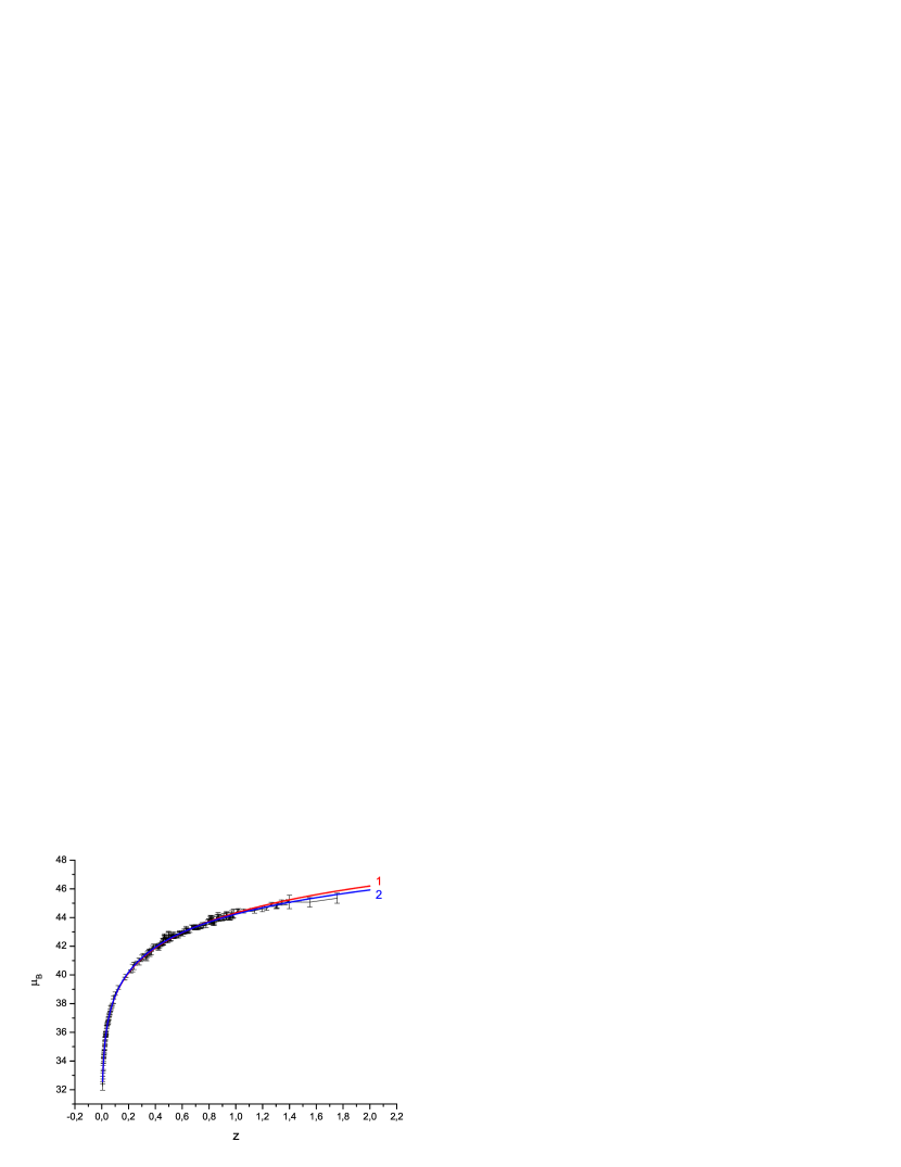
Figure 2: Distant modulii of supernovae SNIa. Smoothed observational data — 211 points. Fitting curves: 1 — $\Lambda$CDM model (IX.16), (IX.17); 2 — $\Lambda$GCDM model (IX.19), (IX.20).

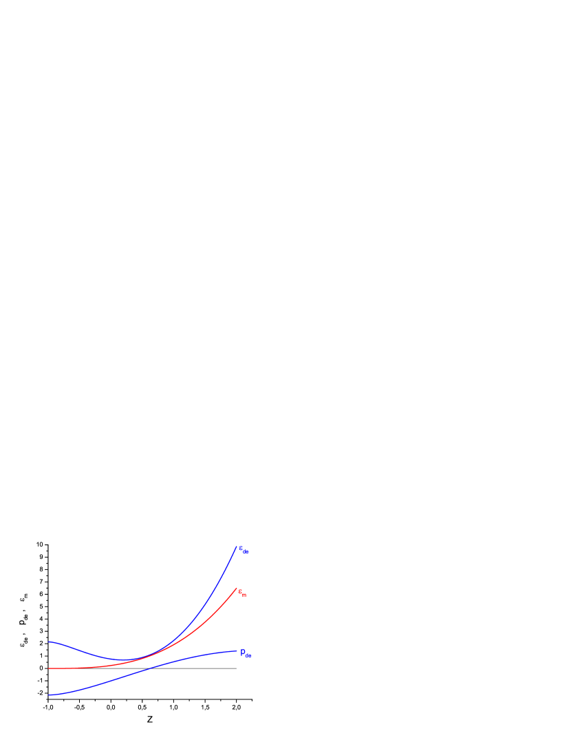
Figure 3: Density and pressure of Dark Energy and density of non–relativistic matter in the region of observations of SNIa and in the future Universe.

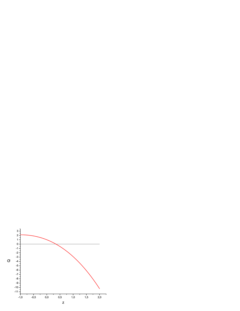
Figure 4: Acceleration of cosmological expansion in the region of observations of SNIa and in the future Universe.

Comparing the results (IX.9) and (IX.16), belonging to $\Lambda$CDM model with the results (IX.12), (IX.13) and (IX.18), (IX.19), belonging to the $\Lambda$GCDM model, it is easy to see that in the framework of the given model the values of parameters obtained from the fits of the original and smoothed data, are statistically equivalent. This fact is not something amazing because the smoothing procedure and the fitting are mathematically related. The use of smoothed data is motivated by the necessity to compare and make a preliminary choice between two different models using the criterion of statistical likelihood.

When the two models are compared, two facts appear. First, the application of the $\chi^{2}$–criterion to the smoothed data of the $\Lambda$GCDM model shows that the model gains a more significant advantage. Second, comparison of (IX.17) and (IX.20) shows that on the smoothed data the intervals of statistical sums are not overlapping, with the lesser value of the statistical sum belonging to the $\Lambda$GCDM model. Therefore, by statistical criteria obtained from the smoothed Hubble diagram for supernovae SNIa, the $\Lambda$GCDM model has an advantage.

In addition to the Hubble diagram for supernovae SNIa, the information about Dark Energy is contained in the Hubble diagram for radio–galaxies RG and gamma–ray bursts GB . It is also contained in the cosmological parameters extracted from the CMB data and correlation functions characterizing the large scale structure of the Universe. Results of processing of the full data set will be reported in a separate paper. Because of big statistical errors of appropriate data, we believe that the use of Hubble diagrams for radio–galaxies and gamma–ray bursts is to no purpose in this work where we discuss statistical criteria to choose between $\Lambda$CDM and $\Lambda$GCDM models. As to the third type of data (following from CMB and correlation functions), we would like to mention the following. Information about the density of Dark Energy on the cosmological scale from the instant of the last scattering $Z_{ls}$ up to the present time is contained in the shift parameter 31

$$\mathcal{R}=\sqrt{\Omega_{{\scriptscriptstyle M}}}\int\limits_{0}^{Z_{ls}}\frac{dz}{\tilde{H}(z)}=1.716\pm 0.062\ .$$ (IX.21)

The (IX.21) parameter can be used under condition that the Dark Energy model, used for the interpretation of SNIa data in the $0<z<2$ interval, can be extrapolated up to $z\sim 1000$. In our view, such an extrapolation (three orders of magnitude for redshifts and nine orders of magnitude for curvature and energy density) looks improbable. In any case, the interpolation $\Lambda$GCDM model is not allowed to be extrapolated in such a way as can be seen from the algorithm of its construction (see Section VIII.2). This is the reason why we do not discuss constraints following from (IX.21). The parameter $\mathcal{A}$ extracted from the acoustic peak data is of a different status. Acoustic oscillations in the photon–baryon plasma prior to recombination give rise to a pick in the correlation function of galaxies. This effect was recently been measured in a sample of luminous red galaxies and leads to the value CMB2

$$\mathcal{A}=\frac{\sqrt{\Omega_{{\scriptscriptstyle M}}}}{Z_{\scriptscriptstyle L\scriptscriptstyle R\scriptscriptstyle G}}\left[\frac{Z_{\scriptscriptstyle L\scriptscriptstyle R\scriptscriptstyle G}}{\tilde{H}(Z_{\scriptscriptstyle L\scriptscriptstyle R\scriptscriptstyle G})}\left(\int\limits_{0}^{Z_{\scriptscriptstyle L\scriptscriptstyle R\scriptscriptstyle G}}\frac{dz}{\tilde{H}(z)}\right)^{2}\right]^{1/3}=0.469\left(\frac{n}{0.98}\right)^{-0.35}\pm 0.017\ ,$$ (IX.22)

where $Z_{\scriptscriptstyle L\scriptscriptstyle R\scriptscriptstyle G}=0.35$ is the redshift at which the acoustic scale has been measured and $n=0.961$ is the spectral index of the primordial power spectrum.

The $\Lambda$GCDM model with the (IX.19) parameters, which were determined from the SNIa data, predicts the following interval for the allowed values of the $\mathcal{A}$ parameter $0.413<\mathcal{A}<0.479$ if the parameter $\Omega_{\scriptscriptstyle M}$ is taken from the allowed interval $0.20<\Omega_{\scriptscriptstyle M}<0.27$. The $\Lambda$GCDM model, which is precisely consistent with the value $\mathcal{A}=0.472$, is as follows

$$\begin{array}[]{c}\displaystyle\chi^{2}/dof=0.93\ ,\qquad\mathcal{M}=43.32\pm 0.02\ ,\qquad 1+z_{0}=1.34\pm 0.03\ ,\\[14.22636pt] \displaystyle\Omega_{\scriptscriptstyle M}=0.26\pm 0.01:\qquad\Omega_{\Lambda}=2.15\pm 0.27\ ,\qquad\Omega_{g}=2.04\pm 0.40\ ,\qquad a_{0}=0.50\pm 0.02\ .\end{array}$$ (IX.23)

The procedure of noise reduction in the Hubble diagram and the obtained results bear, of course, an illustrative character. In fact, we have demonstrated only the near term possibilities of the experiment: i.e. possibility to get the variable component of the Dark Energy and compare the results of the measurements with the prediction of the $\Lambda$GCDM model derived from the exact results of one–loop quantum gravity.

The density and pressure of the Dark Energy and the energy density of non–relativistic matter are plotted in Figure 3. The graphs are calculated by the formulas of $\Lambda$GCDM model (IX.2) with parameters corresponding to $\Omega_{\scriptscriptstyle M}=0.240$ in (IX.19). The acceleration of the Universe, calculated by the formula (IX.1) with the same parameters, is shown in Figure 4. Two features on the graphs in Figure 3 are of special interest: (i) in the entire area of observation of SNIa the density of non–relativistic matter and Dark Energy are compatible in their values; (ii) the density of Dark Energy first decreases with decreasing $z$, and then increases, starting approximately from $z\sim 0.2$. Let us mention the astrophysical aspect of these predictions of the $\Lambda$GCDM model: (i) at the epoch of creation of large scale structures in the Universe, Dark Energy has played a quantitatively important role in the global cosmological dynamics; (ii) the area of relatively small values of redshifts represents significant interest for the observations, because in that area the reconstruction of the graviton–ghost condensate is happening: pre–asymptotic state of the condensate with constant conformal wavelength is transforming into the asymptotic state of the condensate with the constant physical wavelength. With the increasing accuracy of experiments, it is possible that in this area, the nonlinear fluctuations of Dark Energy could be discovered (see SectionV.4).

X Conclusion

From the formal mathematical point of view, the above theory is identical to transformations of equations, determined by the original gauged path integral (II.1), leading to exact solutions for the model of self–consistent theory of gravitons in the isotropic Universe. To assess the validity of the theory, it is useful to discuss again but briefly the three issues of the theory that are missing in the original path integral.

(i) The hypothesis of the existence of classic spacetime with deterministic, but self–consistent geometry is introduced into the theory. It is not necessary to discuss in detail this hypothesis because it simply reflects the obvious experimental fact (region of Planck curvature and energy density is not a subject of study in the theory under discussion). Note, however, that the introduction of this hypothesis into the formalism of the theory leads to a rigorous mathematical consequence: the strict definition of the operation of separation of classical and quantum variables uniquely captures the exponential parameterization of the metric.

(ii) The transfer to the one–loop approximation is conducted in the self–consistent classical and quantum system of equations. Formally, this approximation is of a technical nature because the equations of the theory are simplified only in order to obtain specific approximate solutions. After classical and quantum variables are identified, the procedure of transition to the one–loop approximation is of a standard and known character 7 . In reality, of course, the situation in the theory is much more complex and paradoxical. On the one hand, the quantum theory of gravity is a non–renormalized theory (see, e.g. 36 ). Specific quantitative studies of effects off one–loop approximation are simply impossible. On the other hand, the quantum theory of gravity without fields of matter is finite in the one–loop approximation 3 . The latter means that the results obtained in the framework of one–loop quantum gravity pose limits to its applicability that is mathematically clear and physically significant. The existence of a range of validity for the one–loop quantum gravity without fields of matter is a consequence of two facts. First, there are supergravity theories with fields of matter which are finite beyond the limits of one–loop approximation. Second, the quantum graviton field is the only physical field with a unique combination of such properties as conformal non–invariance and zero rest mass. For this field only there is no threshold for the vacuum polarization and particle creation in the isotropic Universe. Therefore, in the stages of evolution of the Universe, where $H^{2},\ |\dot{H}|\ll m^{2}$ ($m$ is mass of any of the elementary particles), quantum gravitational effects can occur only in the subsystem of gravitons. It is also clear that in any future theory that unifies gravity with other physical interactions, equations of theory of gravitons in one–loop approximation will not be different from those we discuss in this work. Therefore the self–consistent theory of gravitons has the right to lay claim be a reliable description of the most significant quantum gravity phenomena in the isotropic Universe.

(iii) Dynamic properties of ghost fields are captured by the condition of one–loop finiteness of the theory off mass shell of gravitons and ghosts. The class of legitimate gauges picked out by this condition includes gauges that are form–invariant with respect to transformation of the symmetry group of the background geometry. This point is the most nontrivial part of the theory because it is essentially an additional mathematical condition on the theory ensuring its internal consistency. The condition of one–loop finiteness off the mass shell largely determines the mathematical and physical content of the theory. Given that the main results of this work are exact solutions and exact transformations, the evaluation of he proposed approach is reduced to a discussion of this point of the theory. Let us enumerate once more logical and mathematical reasons, forcing us to include the condition of one–loop finiteness off the mass shell into the structure of the theory.

a) Future theory that will unify quantum gravity with the theory of other physical interactions may not belong to renormalizability theories. If such a theory exists, it may only be a finite theory. One–loop finiteness of quantum gravity with no fields of matter that is fixed on the mass shell 3 can be seen as the prototype of properties of the future theory.

b) Because of their conformal non–invariance and zero rest mass, gravitons and ghosts fundamentally can not be located exactly on the mass shell in the real Universe. Therefore, the problem of one–loop finiteness off the mass shell is contained in the internal structure of the theory.

c) In formal schemes, which do not meet the one–loop finiteness, divergences arise in terms of macroscopic physical quantities. To eliminate these divergences, one needs to modify the Lagrangian of the gravity theory, entering quadratic invariants. This, in turn, leads to abandonment of the original definition of the graviton field that generates these divergences. The logical inconsistency of such a formal scheme is obvious. (The mathematical proof of this claim is contained at Appendix XII.2.)

d) In the self–consistent theory of gravitons, one–loop finiteness off the mass shell can be achieved only through mutual compensation of divergent graviton and ghost contributions in macroscopic quantities. The existence of gauges, automatically providing such a compensation, is an intrinsic property of the theory.

From our perspective, the properties of the theory identified in points a), b), c) and d), clearly dictate the need to use only the formulation of self–consistent theory of gravitons, in which the condition of one–loop finiteness off the mass shell (the condition of internal consistency of the theory) is performed automatically. We also want to emphasize that, as it seems to us, the scheme of the theory given below has no alternative both logically and mathematically.

Gauged path integral $\Longrightarrow$ factorization of classic and quantum variables, which ensures the existence of a self–consistent system of equations $\Longrightarrow$ transition to the one–loop approximation, taking into account the fundamental impossibility of removing the contributions of ghost fields to observables $\Longrightarrow$ choice of the ghost sector, satisfying the condition of one–loop finiteness off the mass shell — appears to us logically and mathematically as the only choice.

As part of the theories preserving macroscopic spacetime being clearly one of its components, we see two topics for further discussions. The first of these is the replication of the results of this work by mathematically equivalent formalisms of one–loop quantum gravity. Here we can note that, for example, in the formalism of the extended phase space with BRST symmetry, our results are reproduced, even though the mathematical formalism is more cumbersome. The second topic is the reproduction of our results in more general theories than the one–loop quantum gravity without fields of matter. Here is meant a step beyond the limits of one–loop approximation as well as a description of quantum processes involving gravitons, while taking into account the existence of other quantum fields of spin $J\leqslant 3/2$. In the framework of discussion on this topic, we can make only one assertion: in the one–loop $N=1$ supergravity containing graviton field and one gravitino field, the results of our work are fully retained. This is achieved by two internal properties of $N=1$ supergravity: (i) The sector of gravitons and graviton ghosts in this theory is exactly the same as in the one–loop quantum gravity without fields of matter; (ii) The physical degrees of freedom of gravitino with chiral $h=\pm 3/2$ in the isotropic Universe are dynamically separated from the non–physical degrees of freedom and are conformally invariant; (iii) The gauge of gravitino field can be chosen in such a way that the gravitino ghosts automatically provide one–loop finiteness of $N=1$ supergravity. As for multi–loop calculations in the $N=1$ supergravity and more advanced theoretical models, we have not explored the issue.

Of course, a rather serious problem of the physical nature of ghosts remains. The present work makes use in practice only of formal properties of quantum gravity of Faddeev–Popov–De Witt, which point to the impossibility in principle of removing contributions of ghosts to observable quantities off the mass shell. A deeper analysis undoubtedly will address the foundations of quantum theory. In particular, one should point out the fact that the formalism of the path integral of Faddeev–Popov–De Witt is mathematically equivalent to the assumption that observable quantities can be expressed through derivatives of operator–valued functions defined on the classical spacetime of a given topology. On the other hand, finiteness of physical quantities is ensured in the axiomatic quantum field theory by invoking limited field operators smoothed over certain small areas of spacetime. Extrapolation of this idea to quantum theory of gravity immediately brings up the question on the role of spacetime foam 37 (fluctuations of topology on the microscopic level) in the formation of smoothed operators, and consequently, observable quantities. To make this problem more concrete, a question can be posed on collective processes in a system of topological fluctuations that form the foam. It is not excluded that the non–removable Faddeev–Popov ghosts in ensuring the one–loop finiteness of quantum gravity are at the same time a phenomenological description of processes of this kind.

Study of equations of self–consistent theory of gravitons, automatically satisfying the condition of one–loop finiteness, leads to the discovery of a new class of physical phenomena which are macroscopic effects of quantum gravity. Like the other two macroscopic quantum phenomena of superconductivity and superfluidity, macroscopic effects of quantum gravity occur on the macroscopic scale of the system as a whole, in this case, on the horizon scale of the Universe. Interpretation of these effects is made in terms of gravitons–ghost condensates arising from the interference of quantum coherent states. Each of coherent states is a state of gravitons (or ghosts) with a certain wavelength of the order of the distance to the horizon and a certain occupation number. The vector of the physical state is a coherent superposition of vectors with different occupation numbers.

A key part in the formalism of self–consistent theory of gravitons is played by the BBGKY chain for the spectral function of gravitons, renormalized by ghosts. It is important that equations of the chain may be introduced at an axiomatic level without specifying explicitly field operators and state vectors. It is only necessary to assume the preservation of the structure of the chain equations in the process of elimination of divergences of the moments of the spectral function. Three exact solutions of one–loop quantum gravity are found in the framework of BBGKY formalism. The invariance of the theory with respect to the Wick rotation is also shown. This means that the solutions of the chain equations, in principle, cover two types of condensates: condensates of virtual gravitons and ghosts and condensates of instanton fluctuations.

All exact solutions, originally found in the BBGKY formalism, are reproduced at the level of exact solutions for field operators and state vectors. It was found that exact solutions correspond to various condensates with different graviton–ghost microstructure. Each exact solution we found is compared to a phase state of graviton–ghost medium; quantum–gravity phase transitions are introduced.

We suspect that the manifold of exact solutions of one–loop quantum gravity is not exhausted by three solutions described in this paper. Search for new exact solutions and development of algorithms for that search, respectively, is a promising research topic within the proposed theory. Of great interest will also be approximate solutions, particularly those that describe non–equilibrium and unstable graviton–ghost and instanton configurations.

Self–consistent theory of gravitons allows an easy generalization that takes into account participation of non–relativistic matter in the formation of common self–consistent gravitational field. From the equations of this theory it follows that the era of dominance of non–relativistic matter should be replaced by an era of dominance of graviton–ghost condensate. This result is of direct relevance to the physics of Dark Energy. The pre–asymptotic condition of Dark Energy is interpreted as a condensate of virtual gravitons and ghosts of a constant conformal wavelength. As an asymptotic condition, the theory predicts self–polarized graviton–ghost condensate of constant physical wavelength in the De Sitter space.

The view of the nature of Dark Energy is formulated in the form $\Lambda$GCDM model which interpolates exact solutions of the one–loop quantum gravity. The proposed theory is consistent with existing observational data on Dark Energy extracted from the Hubble diagram for supernovae SNIa. According to the criteria for statistical reliability, the $\Lambda$GCDM model has certain advantages over the $\Lambda$CDM model. A graviton–ghost condensate lays claim to being a variable component of Dark Energy. Result of observational data processing suggests that during the era of large–scale structure formation in the universe, a graviton–ghost condensate played a measurably significant part in shaping global cosmological dynamics.

Further applications of our theory to the physics of Dark Energy will be to conduct numerical experiments with the BBGKY chain, taking into account the non–relativistic matter. The results of these experiments may be able to explain the finer details of the Hubble diagram for supernovae SNIa, which will be identified with increasing completeness and accuracy of observation data. Future observations, in our view, must focus on the variable component of Dark Energy. For reliable identification of this component it is necessary, first move as far as possible into the area of large redshift, and second to explore in detail the area of small red shift, in which, quite possibly, there is a transition from the pre–asymptotic state of graviton–ghost condensate to its asymptotic state.

ACKNOWLEDGMENT. We would like to express our deep appreciation to our friend and colleague Dr. Walter Sadowski for invaluable advise and help in the preparation of the manuscript.

XI APPENDIX I. Cosmological Constant as Energy Density of Equilibrium Vacuum

The cosmological constant in Einstein equations does not contradict the general principles of geometrized gravity theory. Moreover, the gravity theory which includes the $\Lambda$–term looks more natural than a theory without $\Lambda$–term. According to Zeldovitch 20 , $\Lambda$–term is interpreted as the energy density of the vacuum. Today, that definition should be ”updated” a little bit: the subject is the energy density of the equilibrium vacuum subsystems of non–gravitational origin in 4–D space–time: $\varepsilon_{vac}^{(0)}=\Lambda$. The calculation of $\varepsilon_{vac}^{(0)}$ is the task of the future ”Theory of Everything” , based, possibly, on the superstring theory. The existing experimentally verified theory (the Standard Model of quark and leptons interactions) allows making some general conclusions. The most important of these is the fact that for every fundamental physical interaction there is an associated vacuum subsystem with non–zero energy density. They are well–known Higgs condensate in the theory of electro–week interaction and quark–gluon condensate in Quantum Chromodynamics.

The Higgs condensate is forming as a result of spontaneous breaking of electro–week symmetry $U(1)\times SU_{L}(2)$ down to the electromagnetic symmetry $U_{em}(1)$. The energy density of Higgs condensate can be estimated as (in that section $\hbar=1$):

$$\begin{array}[]{c}\displaystyle\varepsilon_{e{\scriptscriptstyle W}}=-\frac{M^{2}_{\scriptscriptstyle H}M^{2}_{\scriptscriptstyle W}}{2g^{2}}-\frac{1}{128\pi^{2}}\left(M^{4}_{\scriptscriptstyle H}+3M^{4}_{\scriptscriptstyle Z}+6M^{4}_{\scriptscriptstyle W}-12M^{4}_{t}\right)\ ,\end{array}$$ (XI.1)

where $M_{\scriptscriptstyle H},\ M_{\scriptscriptstyle Z},\ M_{\scriptscriptstyle W},\ M_{t}$ are masses of Higgs boson, intermediate vector bosons and $t$–quark; $g^{2}=4\pi/29$ is the gauge constant of $SU_{L}(2)$ group on $W$-boson mass–shell. The first term in (XI.1) is the energy density of spatially homogeneous (vacuum) component of the scalar Higgs field $\langle 0|H|0\rangle=v/\sqrt{2}$; the second term is the change of the energy of zero–fluctuations of quantum fields, which have obtained nonzero rest mass from the interaction with the vacuum field $v=246\ \text{GeV}$. Masses of all particles $M\sim v$, therefore

$$\begin{array}[]{c}\displaystyle\varepsilon_{e{\scriptscriptstyle W}}(v)=-\frac{1}{4}\lambda v^{4}\simeq-(120\ \text{GeV})^{4}\ ,\end{array}$$ (XI.2)

where $\lambda$ is a constant or (if high radiation corrections are taken into account) is a very slow function of vacuum field. The numerical value used in (XI.2) corresponds to the mass of Higgs boson $M_{\scriptscriptstyle H}=2M_{\scriptscriptstyle W}\simeq 160\ \text{GeV}$. There is no doubt in the existence of the electro–week vacuum subsystem at the scale $\lambda_{e{\scriptscriptstyle W}}\sim 120\ \text{GeV}$, however a fact that this subsystem is specifically formed by the Higgs mechanism, is not yet experimentally confirmed. A decisive step in that direction would be experimental discovery of the Higgs boson by the LHC.

The quark–gluon condensate is a system of mutually correlated non–perturbative fluctuations, arising during quantum–topological tunnel transitions between degenerated states of gluon vacuum. Energy density of the condensate is

$$\begin{array}[]{c}\displaystyle\varepsilon_{{\scriptscriptstyle Q}{\scriptscriptstyle C}{\scriptscriptstyle D}}=-\frac{b}{32}\langle 0|\frac{\alpha_{s}}{\pi}G_{ik}^{a}G^{ik}_{a}|0\rangle\ ,\\[14.22636pt] \displaystyle b\simeq 9+8T_{g}(m_{u}+m_{d}+0.8m_{s})\simeq 9.6\ ,\end{array}$$ (XI.3)

where

$$\langle 0|\frac{\alpha_{s}}{\pi}G_{ik}^{a}G^{ik}_{a}|0\rangle=u^{4}\simeq(360\ \text{MeV})^{4}$$ (XI.4)

is the main energy–momentum parameter of the quark–gluon condensate; $T_{g}\simeq(1.5\ \text{GeV})^{-1}$ is a characteristic spacetime scale of fluctuations; $m_{u},\ m_{d},\ m_{s}$ are the masses of light quarks. According to the modern paradigm, the quark–gluon condensate has several phase states, in each of which the fluctuations have there own specific microstructure. The value of the parameter, used in (XI.4), refers to the confinement phase of the out–of–hadron vacuum. In that case

$$\varepsilon_{{\scriptscriptstyle Q}{\scriptscriptstyle C}{\scriptscriptstyle D}}(u)=-\frac{b}{32}u^{4}\simeq-(265\ \text{MeV})^{4}$$ (XI.5)

As follows from (XI.2) and (XI.5), the scale of the electro–week vacuum is of the order of $M_{e{\scriptscriptstyle W}}\sim 120\ \text{GeV}$, and the QCD scale is $M_{{\scriptscriptstyle Q}{\scriptscriptstyle C}{\scriptscriptstyle D}}\simeq 265\ \text{MeV}$. The scale $M_{{\scriptscriptstyle D}{\scriptscriptstyle E}}\sim 10^{-12}\ \text{GeV}$, corresponding to the current density of the Dark Energy $\varepsilon_{{\scriptscriptstyle D}{\scriptscriptstyle E}}\sim M^{4}_{{\scriptscriptstyle D}{\scriptscriptstyle E}}$, is not on a pair with $M_{e{\scriptscriptstyle W}},\ M_{{\scriptscriptstyle Q}{\scriptscriptstyle C}{\scriptscriptstyle D}}$. It means that for the high–energy expansions of the Standard Model, the vacuum is of a more complicated structure. First, there should be vacuum subsystems with positive energy density; Second, the theory should contain mechanisms of mutual compensation of the contributions from different vacuum subsystems to the full energy density of the equilibrium vacuum.

The Standard Model, when applied to the description of the cosmological vacuum and cosmological plasma of elementary particles, forecasts that the vacuum subsystems (XI.1), (XI.3) are of evolutionary origin. The energy density of these subsystems is not constant by the definition. Higgs’ and quark–gluon condensates appear in the early Universe in the processes of relativistic phase transitions. The energy density of the vacuum is a functional of non–equilibrium parameters $\mathcal{V}\neq v$, $\mathcal{U}\neq u$:

$$\varepsilon_{vac}(\mathcal{V},\mathcal{U})=\Lambda_{0}+\varepsilon_{e{\scriptscriptstyle W}}(\mathcal{V})+\varepsilon_{{\scriptscriptstyle Q}{\scriptscriptstyle C}{\scriptscriptstyle D}}(\mathcal{U})\ ,$$ (XI.6)

where $\Lambda_{0}=const$ is the energy density of the vacuum at the evolutionary stage before the electro–week transition. In the areas of phase transitions, functions $\varepsilon_{e{\scriptscriptstyle W}}(\mathcal{V})$ and $\varepsilon_{{\scriptscriptstyle Q}{\scriptscriptstyle C}{\scriptscriptstyle D}}(\mathcal{U})$ are changing from zero values to equilibrium values given in (XI.2) and (XI.5). The characteristic transition times and the times of relaxations of vacuum subsystems to the equilibrium states are incommensurably shorter than the characteristic times of the Universe evolution. By that reason, almost immediately after the phase transition, one might talk about the contributions of the respective condensates of the Standard Model to the cosmological constant. After the quark–hadron transition, we have the current value of the non–gravitational contributions to $\Lambda$–term:

$$\Lambda=\Lambda_{0}+\varepsilon_{e{\scriptscriptstyle W}}(v)+\varepsilon_{{\scriptscriptstyle Q}{\scriptscriptstyle C}{\scriptscriptstyle D}}(u)\ .$$ (XI.7)

Thus, the theory of fundamental interactions, particularly, the Standard Model, leads to the conclusion that the treatment of the cosmological constant as an energy density of the equilibrium vacuum, is related to the late stages of the Universe evolution, situated on the cosmological scale after all the relativistic phase transitions in the vacuum and in the plasma of elementary particles are completed.

Inevitability of the ”fine tuning” of different vacuum subsystems, with the result that the asymptotical value of the cosmological constant (XI.7) turns out to be very small or even equal to zero, is actually the experimental fact, resulting from the very existence of the modern Universe. Actually, without the ”fine tuning” any of the phase transitions from the Standard Model will lead either to the collapse of the Universe, or to the exponential inflation, preventing the formation of large–scale structures. At the same time, strong inequality $|\varepsilon_{e{\scriptscriptstyle W}}(v)|\gg|\varepsilon_{{\scriptscriptstyle Q}{\scriptscriptstyle C}{\scriptscriptstyle D}}(u)|$ forces us to consider separately the problem of the ”fine tuning” at the electro–week and QCD scales.

The compensation of the energy of the Higgs condensate (XI.1) at the fundamental level can, in principle, be provided by the supersymmetry of particles and interactions. Unfortunately, in the superstring scenarios of the ”Theory of everything” , the effective algorithms to develop that kind of theory are absent at the present time. The supersymmetry, if it actually exists in Nature, is strongly broken, but the mechanisms of destruction, it seems, are not spontaneous and 4–D spacetime is not an arena of an action of these mechanisms. It is not excluded, that the reduction of the ”Theory of Everything” to the low–energy Standard Model is provided by physical phenomena working in the extra spatial dimensions. Experimental test of the supersymmetry, as a realistic concept of the elementary particle physics, will be conducted at LHC. The discussion about the compensation mechanisms for the energy density of Higgs condensate (XI.1) should continue after the results of the experiments start arriving.

Supersymmetry has no relation to the problem of compensation of the quark–gluon condensate (XI.3). We think the problem should be solved in the framework of low–energy physics of strong interactions. One of the possible approaches is to assume that at the QCD scale there are additional contributions to (XI.3), and the sum turns to zero due to the tuning of QCD parameters. The discussion of these scenarios is out of the scope of the current work.

The hypothesis about the mutual compensations of non–gravitational contributions to the $\Lambda$–term do not remove the questions regarding the final value of $\Lambda\neq 0$, which is in agreement with observed data. At the order–of–value estimations, $\Lambda$–term, with its value equal to the modern Dark Energy density, satisfies Zeldovitch’s relationship 22 with the Kardashev’s modification 38

$$\varepsilon_{{\scriptscriptstyle D}{\scriptscriptstyle E}}\sim\Lambda=\frac{m_{\pi}^{6}}{(2\pi)^{4}M_{Pl}^{2}}=3\times 10^{-47}\ \text{GeV}^{4}\ ,$$ (XI.8)

where $m_{\pi}=138\ \text{MeV}$ — pion mass; $M_{Pl}=1.22\cdot 10^{19}\ \text{GeV}$ — Planck mass. As it is known, the pion mass is an object of non–perturbative QCD. Therefore, in formula (XI.8) the observed density of Dark Energy is expressed only via the combination of minimal $\Lambda_{{\scriptscriptstyle Q}{\scriptscriptstyle C}{\scriptscriptstyle D}}\simeq 2m_{\pi}$ and maximal scales $M_{Pl}$ of the elementary particle physics. Adopting also the Sakharov’s idea of Einstein equations modification by the effect of gravitational exchange interaction of identity particles 39 , we may suggest that the energy density of vacuum (XI.8) is formed by the gravitational exchange interaction of quantum–topological fluctuations in the hadron vacuum. This idea leads to a formula

$$\varepsilon^{(grav)}_{{\scriptscriptstyle Q}{\scriptscriptstyle C}{\scriptscriptstyle D}}\sim\Lambda=\frac{\pi T_{g}^{2}}{2M_{Pl}^{2}}|\varepsilon_{{\scriptscriptstyle Q}{\scriptscriptstyle C}{\scriptscriptstyle D}}|^{2}\ln^{2}\frac{T_{g}^{-1}}{\Lambda_{{\scriptscriptstyle Q}{\scriptscriptstyle C}{\scriptscriptstyle D}}}=4\times 10^{-43}\ \text{GeV}^{4}\ .$$ (XI.9)

The difference of four orders between values (XI.8) and (XI.9) is no any longer a catastrophe for the theory (see formula (XI.10) below).

The nature of the cosmological constant discussed above, (more precisely, the contributions to the energy density of the vacuum controlled by the modern theory of elementary particles), suggests a set of interesting analogies. First, because the vacuum subsystems of electromagnetic, week and strong interactions are known from experiments, it is appropriate to ask a question: what is the vacuum subsystem connected with the fundamental gravitational interaction? We hope that an answer is provided in our work: the existence of the graviton–ghost condensate, i.e. the Dark Energy, is a direct consequence of applying the first principles of quantum theory of gravitation. The second analogy is in the fact that all vacuum subsystems are the subjects of evolution as Universe progresses, and the asymptotical states appear as results of relativistic phase transitions. From the evolutional criterion, the difference between graviton–ghost vacuum subsystem and non–gravitational vacuum subsystems is of a quantitative character only. Non–gravitational vacuum subsystems relax on the respective characteristic scales of elementary particle physics, while due to the weakness of gravitational interaction, the graviton–ghost condensate relaxation takes place at the time intervals which are of the order the age of the Universe. Finally, the third general property of all vacuum subsystems is that the vacuum energy density in the asymptotical (equilibrium) state acquires a constant value. It is worth mentioning that the graviton–ghost condensate in its equilibrium state, as well the vacuum of QCD, is of the instanton microstructure.

Of course, the problem of mutual compensation of different contributions to the energy density of non–gravitational vacuum subsystems remains unsolved. However, we believe that the consideration of the graviton–ghost component of the physical vacuum somewhat reduces the magnitude of the problem. Actually, as shown at the end of the section VI.2, the mathematical structure of the self–consistent theory of gravitons itself possesses an effective renormalization procedure applied to the energy density of non–gravitational vacuum by virtue of the graviton–ghost contributions. The possibility of such renormalization is here regardless of the sign of the $\Lambda$–term. Particularly, the renormalization of $\Lambda$–term (XI.9), formed by the gravitational exchange interactions of non-perturbative quark–gluon fluctuations, is conducted by formula (VI.34) and leads to the result:

$$\varepsilon^{(\infty)}_{vac}=\sqrt{\frac{3\pi}{4|N_{g}|}}T_{g}M_{Pl}|\varepsilon_{{\scriptscriptstyle Q}{\scriptscriptstyle C}{\scriptscriptstyle D}}|\ln\frac{T_{g}^{-1}}{\Lambda_{{\scriptscriptstyle Q}{\scriptscriptstyle C}{\scriptscriptstyle D}}}=\frac{10^{17}}{\sqrt{N_{g}}}\ \text{GeV}^{4}\ .$$ (XI.10)

As follows from (XI.10), $\varepsilon^{(\infty)}_{vac}\sim 10^{-46}\ \text{GeV}^{4}$ with $|N_{g}|\sim 10^{126}$. Unfortunately, the question regarding the concordance of the graviton–ghost condensate’s parameter $|N_{g}|$ with the numerical values of parameters of a different physical nature (example (XI.10), with QCD parameters), remains open. But in that case one always may appeal to the anthropic principle.

XII APPENDIX II. Renormalizations and Anomalies

The problem of calculating the anomalies in the energy-momentum tensor of gravitons (quantum field with spin $J=2$) was discussed in 37 ; 46 ; 47 . A large number of works are devoted to the study of graviton quantum field in De Sitter space. Here we provide only some links. In some works 48 ; 49 the non–ghost models were considered; in other works 50 ; 51 the ghost fields with harmonic gauge were taken into account. Common feature of all known versions of quantum theory of gravitons in the isotropic Universe is the lack of one–loop finiteness off the mass shell.

In Sections XII.1, XII.2 we discuss a self–consistent theory of gravitons in isotropic Universe with the ghost sector not taken into account. As has been repeatedly stated, we believe that such a model is not mathematically sound. Gauges, completely removing the degeneracy, are absent in the theory of gravity. Thus, in the self–consistent theory of gravitons the ghost sector is inevitable present. Now, however, let us assume for the moment that the self–consistent theory of gravitons without ghosts is worth at least as a model of mathematical physics. The purpose of this Section is to get the properties of this model and to show that it is mathematically and physically internally inconsistent. Note also that the self–consistent theory of gravitons in the harmonic gauge (III.79) has qualitatively the same status as the non–ghost model: the one–loop non–renormalizability is hindering the attempts to obtain definitive results within this theory.

XII.1 Gravitons with no Ghosts. Vacuum Einstein Equations with Quantum Logarithmic Corrections

It clear from the outset that in the non–ghost model the calculation of observables will be accompanied by the emergence of divergences. It is therefore necessary to formulate the theory in such a way that the regularization and renormalization operations are to be contained in its mathematical structure from the very beginning. We talk here about changes in the mathematical formulation of the theory. The relevant operations should be introduced into the theory with care: first, in the amended theory, coexistence of classical and quantum equations should be ensured automatically; second, the enhanced theory should not contain objects initially missing from the theory of gravity.

The dimensional regularization satisfies both above–mentioned conditions. Important, however, is the following fact: the use of dimensional regularization suggests that the self–consistent theory of gravitons in the isotropic Universe is originally formulated in a spacetime of dimension $D=1+d$, where $1$ is the dimension of time; $d=3-2\varepsilon$ is the dimension of space. The special status of the time is due to the two factors: (i) all the events in the Universe, regardless of its actual dimension, are ordered along the one–dimensional temporal axis; (ii) the canonical quantization of the graviton field in terms of the commutation relations for generalized coordinates and generalized momenta also presuppose the existence of the one–dimensional time. As for the space dimension, the limit transition to the true dimension $d=3$ is implemented after the regularization and renormalization.

Thus, we are working in a space with a metric

$$\begin{array}[]{c}\displaystyle ds^{2}=a^{2}(\eta)(d\eta^{2}-\gamma_{\alpha\beta}dx^{\alpha}dx^{\beta})\ ,\qquad\gamma^{\alpha\beta}\gamma_{\alpha\beta}=d\ ,\\[14.22636pt] \displaystyle\sqrt{|g_{(d)}|}=a^{d+1}\ ,\qquad R_{(d)}=-\frac{d}{a^{2}}\left(2\frac{a^{\prime\prime}}{a}+(d-3)\frac{a^{{}^{\prime}2}}{a^{2}}\right)\ .\end{array}$$ (XII.1)

To avoid mathematical contradictions that could arise at the limit $d\to 3$, Einstein equations in $D$-dimensional spacetime should be written down in exactly the form in which they were obtained from the variational principle:

$$\begin{array}[]{c}\displaystyle\frac{1}{\varkappa_{d}}\sqrt{|g_{(d)}|}\left(R_{0(d)}^{0}-\frac{1}{2}R_{(d)}\right)\equiv\\[14.22636pt] \displaystyle\frac{1}{2\varkappa_{d}}d(d-1)a^{d-3}{a^{\prime}}^{2}=\frac{1}{8\varkappa_{d}}a^{d-1}\sum_{{{\bf k}\sigma}}\langle\Psi_{g}|\hat{\psi}_{{\bf k}\sigma}^{+^{\prime}}\hat{\psi}^{\prime}_{{\bf k}\sigma}+k^{2}\hat{\psi}_{{\bf k}\sigma}^{+}\hat{\psi}_{{\bf k}\sigma}|\Psi_{g}\rangle\ ,\\[14.22636pt] \displaystyle-\frac{d-1}{2\varkappa_{d}}\sqrt{|g_{(d)}|}R_{(d)}\equiv\\[14.22636pt] \displaystyle\frac{1}{2\varkappa_{d}}d(d-1)\left[2a^{d-2}{a^{\prime\prime}}+(d-3)a^{d-3}{a^{\prime}}^{2}\right]=-\frac{d-1}{8\varkappa_{d}}a^{d-1}\sum_{{{\bf k}\sigma}}\langle\Psi_{g}|\hat{\psi}_{{\bf k}\sigma}^{+^{\prime}}\hat{\psi}^{\prime}_{{\bf k}\sigma}-k^{2}\hat{\psi}_{{\bf k}\sigma}^{+}\hat{\psi}_{{\bf k}\sigma}|\Psi_{g}\rangle\ ,\end{array}$$ (XII.2)

$$\hat{\psi}^{\prime\prime}_{{\bf k}\sigma}+(d-1)\frac{a^{\prime}}{a}\hat{\psi}^{\prime}_{{\bf k}\sigma}+k^{2}\hat{\psi}_{{\bf k}\sigma}=0\ .$$ (XII.3)

Here $\varkappa_{d}$ is the Einstein gravitational constant in $D$–dimensional spacetime. (Dimension $[\varkappa_{d}\hbar]=[l]^{D-2}$.) The left hand sides of equations (XII.2) satisfy the Bianchi identity:

$$\begin{array}[]{c}\displaystyle\frac{1}{2\varkappa_{d}}d(d-1)\left[a^{d-3}{a^{\prime}}^{2}\right]^{\prime}-\frac{1}{2\varkappa_{d}}d(d-1)\frac{a^{\prime}}{a}\left[2a^{d-2}{a^{\prime\prime}}+(d-3)a^{d-3}{a^{\prime}}^{2}\right]\equiv 0\ .\end{array}$$ (XII.4)

In the right hand side of equations (XII.2), the identity (XII.4) generates condition of the graviton EMT conservation that satisfies if the equations of motion (XII.3) are taken into account. Regarding the origin of the system of equations (XII.2) and (XII.3), we should make the following comment. In this case it is inappropriate to invoke the reference to the path integral and factorization of its measures because the path integral inevitably leads to the theory of ghosts interacting with the macroscopic gravity. We can only mention a heuristic recipe: one should refer to the density of Einstein equations with mixed indices, define the exponential parameterization of the metric, and expand the equations into a series of metric fluctuations with an accuracy of the second–order terms. Deviations from this recipe (for example, linear parameterization $\hat{g}_{ik}=g_{ik}+\hat{h}_{ik}$) lead to a system of inconsistent classical and quantum equations. To remove this sort of inconsistency, one is forced to use artificial transactions outside the formalism of the theory (see, for example, 42 ).

While working with the system of equations (XII.2), (XII.3), we face with two mathematical problems. The first problem is that in the framework of that system of equations, except in very special cases, it is impossible to formulate the dynamics of operators on a given background that is to get the solution of the equation (XII.3) as an accurate operator function of time. This is due to the fact that formulae of (XII.2) in reality are not yet specific equations. They are only a layout of Einstein equations with radiation corrections. These equations can only be obtained after regularization and renormalizations of the ultraviolet divergences. In addition, the functional form of equations depends on which quantum gravitational effects are to be taken into account outside the sector of vacuum (i.e. zero) fluctuations of the graviton field. The only possible way to study the system of equations (XII.2) and (XII.3) is (i) to obtain the solution of operator equation (XII.3) in a form of a functional of the scale factor without specifying the dependence on $a(\eta)$ with a clear emphasis on zero fluctuations in this functional, (ii) to substitute the obtained functional in (XII.2) under certain assumptions about the state vector; (iii) to regularize and renormalize and finally (iv) to solve the macroscopic Einstein equations, obtained after these operations. Implementation of the program, an essential element of which is the allocation of zero fluctuations generating ultraviolet divergences, is possible only when using the method of asymptotic expansions of solutions of operator equation in the square of wavelength of the graviton modes. Thus, the problem of the lack of macroscopic Einstein equations in the original formulation of this theory with divergences limits the methods of this theory to the short–wave approach. Note that this fact was clearly indicated by DeWitt 7 .

The second problem is related to the infrared instability of the theory, with the object of the theory being a conformal non–invariant massless quantum field. The problem is due to the fact that not every representation of the asymptotic series can be substituted into energy–momentum tensor to perform the summation over the wave numbers. For example, if in the explicit form, a term in the asymptotic series contains a large parameter $k^{2n}$ in the denominator, then starting from $n=2$ in the integration over the wave numbers the infrared divergences will appear. Such an asymptotic series can not be used even for the renormalization of ultraviolet divergences, because when it is used in the space of the physical dimension $d=3$, the logarithmic divergences arise simultaneously at the ultraviolet and the infrared limits. In the method of dimensional regularization the problem is reduced to the fact that it is impossible to choose an interim dimension $d$ in a way such that the integral exists at both limits.

Formally, the technical problem described above is partly solved by reformatting the asymptotic series. In particular, the following method will be used, in which parameter of the asymptotic expansion is the effective frequency

$$\omega_{k}^{2}=k^{2}+\rho\ ,\qquad\rho=\frac{d-1}{4d}a^{2}R_{(d)}=-\frac{d-1}{4}\left[2\frac{a^{\prime\prime}}{a}+(d-3)\frac{a^{{}^{\prime}2}}{a^{2}}\right]\ .$$ (XII.5)

In this method, the integrals over the wave numbers can be defined in terms of the principal value. Contributions of the poles at $k=\sqrt{-\rho}$ can not be mathematically verified if only because there are such contributions from each term of the infinite asymptotic series. The inability to describe infrared effects is the principal disadvantage of a theory with divergences, which uses only asymptotic expansions with respect to the wavelength. Meanwhile, as general considerations and the results of this work show, in the physics of conformal non–invariant massless field the most interesting and innovative effects occur in the infrared spectrum. The method of describing these effects, based on the exact BBGKY chain, can not be used in the theory with divergences, because a method regularizing the infinite chain of moments of the spectral function does not exist.

The above problems automatically reduces the interest toward the theory with divergences. However, given that all previous works in this area have been implemented in the framework of regularization and renormalization, let us conduct our analysis to the end. In calculations, it is enough to consider the equation for the convolution. After identity transformations, using the equation of motion (XII.3), we get

$$\begin{array}[]{c}\displaystyle\frac{1}{2\varkappa_{d}}d(d-1)\left[2a^{d-2}{a^{\prime\prime}}+(d-3)a^{d-3}{a^{\prime}}^{2}\right]=-\frac{d-1}{16\varkappa_{d}}\sum_{{{\bf k}\sigma}}\left(W^{\prime}_{{\bf k}\sigma}a^{d-1}\right)^{\prime}\ ,\end{array}$$ (XII.6)

where

$$W_{{\bf k}\sigma}=\langle\Psi_{g}|\hat{\psi}_{{\bf k}\sigma}^{+}\hat{\psi}_{{\bf k}\sigma}|\Psi_{g}\rangle$$

is the spectral function of gravitons. The calculation of the spectral function by the method of asymptotic expansion with respect to the square of wavelength was described in Section IV.1. Now we need to repeat this calculation excluding the ghosts, but with input from zero fluctuations in the spacetime of dimension $D=d+1$. The relevant calculations do not require additional comments. A spectral function is represented as:

$$W_{{\bf k}\sigma}=W^{(vac)}_{{\bf k}\sigma}+W^{(exc)}_{{\bf k}\sigma}\ ,$$ (XII.7)

where $W^{(vac)}_{{\bf k}\sigma}$ is the vacuum component of the spectral function and $W^{(exc)}_{{\bf k}\sigma}$ is the spectral function of excitations. After passage to the limit $d\to 3$, the contribution of $W^{(exc)}_{{\bf k}\sigma}$ to the EMT of short gravitons is exactly the same as (IV.9), (IV.10). In the future, we discuss only the contribution from vacuum components of the spectral function. In the calculations, we must keep in mind that in the $d$–dimensional space the number of internal degrees of freedom of transverse gravitons is $w_{g}=(d+1)(d-2)/2$. The solution for the vacuum spectral function is expressed in terms of the functional (IV.4):

$$\sum_{\sigma}W^{(vac)}_{{\bf k}\sigma}=\frac{4\varkappa_{d}\hbar}{a^{d-1}}\cdot\frac{(d+1)(d-2)}{4\epsilon_{k}}=\frac{4\varkappa_{d}\hbar}{a^{d-1}}\cdot\frac{(d+1)(d-2)}{4\omega_{k}}\sum_{s=0}^{\infty}(-1)^{s}\hat{J}_{k}^{s}\cdot 1\ ,$$ (XII.8)

The powers of operator $\hat{J}_{k}^{s}\cdot 1$ are defined by formulas (IV.5), in which $\omega_{k}^{2}$ has the form (XII.5). After substitution of (XII.8) into (XII.6), the zero–term in the asymptotic expansion creates an integral, calculated by the rules of dimensional regularization:

$$\sum_{{\bf k}}\frac{1}{\omega_{k}}=\frac{1}{(2\pi)^{d}}\frac{2\pi^{d/2}}{\Gamma(d/2)}\int\limits_{0}^{\infty}\frac{k^{d-1}dk}{(k^{2}+\rho)^{1/2}}=\frac{\displaystyle\Gamma\left[(3-d)/2\right]}{\displaystyle 2^{d-1}\pi^{(d+1)/2}(1-d)}\rho^{(d-1)/2}\ .$$ (XII.9)

The $\Gamma-$function in (XII.9) diverges for $d\to 3$. Therefore, calculation of the integral (XII.9) and transformation of expressions with $\Gamma-$functions are carried out with those values of $d$ which provide the existence of the integral and $\Gamma-$functions. At the final stage, the result of these calculations is analytically continued to the vicinity $d=3$. All other terms of the asymptotic expansion (XII.8) generate finite integrals and do not require a dimensional regularization. For reasons of heuristic rather than mathematical nature, it is considered that these terms are negligible compared to the contribution of the principal term of the asymptotic expansion (see below the effective Lagrangian (XII.19)). Convolution of $D$–dimensional Einstein’s equations (XII.6), containing the main term of the vacuum EMT of gravitons, has the form:

$$\begin{array}[]{c}\displaystyle\frac{1}{2\varkappa_{d}}d(d-1)\left[2a^{d-2}{a^{\prime\prime}}+(d-3)a^{d-3}{a^{\prime}}^{2}\right]=\frac{\hbar(d+1)(d-2)}{2^{d+3}\pi^{(d+1)/2}}\Gamma\left(\frac{3-d}{2}\right)\left[\left(\frac{\rho^{(d-1)/2}}{a^{d-1}}\right)^{\prime}a^{d-1}\right]^{\prime}\ .\end{array}$$ (XII.10)

Other Einstein equations can be obtained using the Bianchi identities. A complete system of Einstein vacuum equations is written in $D$–covariant form:

$$\begin{array}[]{c}\displaystyle R_{i(d)}^{k}-\frac{1}{2}\delta_{i}^{k}R_{(d)}+\\[14.22636pt] \displaystyle+\frac{\varkappa_{d}\hbar(d+1)(d-2)(d-1)^{\frac{d-1}{2}}}{2^{2d+2}(d\pi)^{\frac{d+1}{2}}}\Gamma\left(\frac{3-d}{2}\right)\left[\left(R_{(d)}^{\frac{d-1}{2}}\right)^{;k}_{;i}-\delta_{i}^{k}\left(R_{(d)}^{\frac{d-1}{2}}\right)^{;l}_{;l}-\left(R_{i(d)}^{k}-\frac{1}{d+1}\delta_{i}^{k}R_{(d)}\right)R_{(d)}^{\frac{d-1}{2}}\right]=0\ .\end{array}$$ (XII.11)

Equation (XII.11) are obtained by the variation of action

$$\begin{array}[]{c}\displaystyle S_{vac}=\int\sqrt{|g_{(d)}|}d^{\scriptscriptstyle D}x\left[-\frac{1}{2\varkappa_{d}}R_{(d)}+\frac{\hbar(d-2)(d-1)^{\frac{d-1}{2}}}{2^{2d+2}(d\pi)^{\frac{d+1}{2}}}\Gamma\left(\frac{3-d}{2}\right)R_{(d)}^{\frac{d+1}{2}}\right]\ .\end{array}$$ (XII.12)

It is obvious from (XII.11), (XII.12) that the method of dimensional regularization retains overall covariance of the theory. Of course, quantum corrections, appearing in (XII.11), satisfy the condition of conservation.

Renormalization and removal of regularization (limit $d\to 3$) are held at the level of action. A parameter with the dimension of length, which will eventually acquire the status of renormalization scale, is contained within the theory. This parameter, referred to as $L_{g}$, is appears in the $D$–dimensional constant of gravity:

$$\varkappa_{d}=\varkappa\cdot L_{g}^{d-3}\ .$$ (XII.13)

The technique of removal the regularization assumes conservation of dimensionality for those objects in which the limit operation is performed. There are two such objects: the measure of integration $d\mu$ and the density of the Lagrangian $\mathcal{L}$. As can be seen from (XII.12), (XII.13), the first (Einstein) term of the action is written down as

$$\begin{array}[]{c}\displaystyle S^{(1)}_{vac}=\int\mathcal{L}^{(1)}d\mu\ ,\\[14.22636pt] \displaystyle\mathcal{L}^{(1)}=-\frac{1}{2\varkappa}R_{(d)}\ ,\qquad d\mu=\sqrt{|g_{(d)}|}L_{g}^{4-D}d^{D}x\ ,\end{array}$$ (XII.14)

where $D$–dimensional objects $\mathcal{L}$ and $d\mu$ have the same dimensions as the corresponding 4–dimensional objects. In this sector of the theory the limit transition is trivial: $R_{(d)}\to R$, $d\mu\to\sqrt{-g}d^{4}x$. In the sector of quantum corrections to the Einstein theory, we introduce the same measure and obtain the density of the Lagrangian:

$$\mathcal{L}^{(2)}=\frac{\hbar L_{g}^{d-3}(d-2)(d-1)^{\frac{d-1}{2}}}{2^{2d+2}(d\pi)^{\frac{d+1}{2}}}\Gamma\left(\frac{3-d}{2}\right)R_{(d)}^{\frac{d+1}{2}}$$ (XII.15)

It is necessary to emphasize that the operations of renormalizations and removal of regularization have to be mathematically well–defined and generally–covariant. The condition of mathematical certainty assumes that the renormalization is conducted before the lifting of regularization. At the same time, the general–covariance of the procedure is automatically fulfilled if the counter–terms imposed in the Lagrangian are the $D$–dimensional invariants. Note also that if the mathematical value is finite at $d=3$, then the above formulated conditions do not prevent the expansion of this quantity in a Taylor series over the parameter $(3-d)/2$. In particular, we can write:

$$\begin{array}[]{c}\displaystyle L_{g}^{d-3}R_{(d)}^{\frac{d+1}{2}}\equiv R_{(d)}^{2}\left(L_{g}^{2}R_{(d)}\right)^{\frac{d-3}{2}}=R_{(d)}^{2}\left(1+\frac{3-d}{2}\ln\frac{\mu_{g}^{2}}{R_{(d)}}+...\right)\ ,\end{array}$$ (XII.16)

where $\mu_{g}=1/L_{g}$; ellipsis designate the terms which do not contribute to the final result. The substitution (XII.16) in (XII.15) provides:

$$\mathcal{L}^{(2)}=\frac{\hbar(d-2)(d-1)^{\frac{d-1}{2}}}{2^{2d+2}(d\pi)^{\frac{d+1}{2}}}\Gamma\left(\frac{3-d}{2}\right)R_{(d)}^{2}+\frac{\hbar(d-2)(d-1)^{\frac{d-1}{2}}}{2^{2d+2}(d\pi)^{\frac{d+1}{2}}}\Gamma\left(\frac{5-d}{2}\right)R_{(d)}^{2}\ln\frac{\mu_{g}^{2}}{R_{(d)}}+...\ .$$ (XII.17)

According to (XII.17), the source Lagrangian of the theory requires a $D$–invariant counter–term, which removes the contribution proportional to the diverging $\Gamma$–function:

$$\mathcal{L}_{0}^{(2)}=-\frac{\hbar(d-2)(d-1)^{\frac{d-1}{2}}}{2^{2d+2}(d\pi)^{\frac{d+1}{2}}}\Gamma\left(\frac{3-d}{2}\right)R_{(d)}^{2}+\frac{\hbar}{4f^{2}}R_{(d)}^{2}\ .$$ (XII.18)

In (XII.18), there is a new finite constant of the theory of gravity $1/f^{2}$. The removal of the regularization in the renormalized Lagrangian is conducted by the regular transition:

$$\begin{array}[]{c}\displaystyle\mathcal{L}_{ren}=\lim_{d\to 3}\left(\mathcal{L}^{(1)}+\mathcal{L}^{(2)}+\mathcal{L}^{(2)}_{0}\right)=\\[14.22636pt] \displaystyle=-\frac{1}{2\varkappa}R+\frac{\hbar}{4f^{2}}R^{2}+\frac{\hbar}{1152\pi^{2}}R^{2}\ln\frac{\mu_{g}^{2}}{R}=-\frac{1}{2\varkappa}R+\frac{\hbar}{1152\pi^{2}}R^{2}\ln\frac{\lambda_{g}^{2}}{R}\ ,\end{array}$$ (XII.19)

where

$$\lambda_{g}^{2}=\mu_{g}^{2}\exp\frac{288\pi^{2}}{f^{2}}$$

is the renorm–invariant scale. There is a heuristic argument allowing to use the obtained expression: quantum corrections in the Lagrangian ( ref (12.19)) dominate over all other neglected terms of the asymptotic series over The logarithmic parameter $\ln(\lambda_{g}^{2}/R)\gg 1$.

The renormalized Einstein vacuum equations with quantum corrections obtained from the Lagrangian (XII.19) are as follows:

$$\begin{array}[]{c}\displaystyle R_{i}^{k}-\frac{1}{2}\delta_{i}^{k}R+\\[14.22636pt] \displaystyle+\frac{\varkappa\hbar}{288\pi^{2}}\left\{\left[R\ln\frac{\lambda_{g}^{2}}{R}\right]_{;i}^{;k}-\delta_{i}^{k}\left[R\ln\frac{\lambda_{g}^{2}}{R}\right]_{;l}^{;l}-\left(RR_{i}^{k}-\frac{1}{4}\delta_{i}^{k}R^{2}\right)\ln\frac{\lambda_{g}^{2}}{R}-\frac{1}{8}\delta_{i}^{k}R^{2}\right\}=0\ .\end{array}$$ (XII.20)

Note that exactly the same equations are obtained from $D$–dimensional equations (XII.11), provided that the operations are performed in the same sequence: first a renormalization with the introduction of $D$–covariant counter–terms is conducted, and then a limit transition to the physical dimension is performed.

XII.2 Intrinsic Contradiction of Theory with no Ghosts: Impossibility of One-Loop Renormalization

We are still discussing a formal model — self–consistent theory of gravitons with no ghosts. In the previous section it was shown that the renormalization of divergences, that inevitably arise in this model, requires the imposition of an additional term quadratic in the curvature in the Lagrangian. It is now necessary to draw attention to two mathematical facts: (i) the need for a modification of Einstein theory is caused by quantum effects contained in the Lifshitz operator equation (XII.3); (ii) the original Lagrangian and operator equations of the modified theory have the form:

$$\begin{array}[]{c}\displaystyle\mathcal{L}=\int\left(-\frac{1}{2\varkappa}\hat{R}+\frac{\hbar}{4f^{2}}\hat{R}^{2}\right)\sqrt{-\hat{g}}d^{4}x\ ,\end{array}$$ (XII.21)

$$\begin{array}[]{c}\displaystyle\sqrt{-\hat{g}}\left[\frac{1}{\varkappa}\left(\hat{R}_{i}^{k}-\frac{1}{2}\delta_{i}^{k}\hat{R}\right)+\frac{\hbar}{f^{2}}\left(\hat{D}_{i}\hat{D}^{k}\hat{R}-\delta_{i}^{k}\hat{D}_{l}\hat{D}^{l}\hat{R}-\hat{R}\hat{R}_{i}^{k}+\frac{1}{4}\delta_{i}^{k}\hat{R}^{2}\right)\right]=0\ ,\end{array}$$ (XII.22)

where $\hat{D}_{i}$ is a covariant derivative in a space with the operator metric $\hat{g}_{ik}$. It is quite obvious that these facts contradict each other: the quantum effects in the Lifshitz equation lead to a theoretical model that contradicts the Lifshitz equation. Let us demonstrate that the contradiction is a direct consequence of the non–renormalizability of the model (XII.21) off the graviton mass shell.

Equations (XII.22), after their linearization describe quantized waves of two types — tensor and scalar. It makes sense to discuss the problem of the scalar modes only in the event that at least preliminary criteria for consistency of modified theory will be obtained. Therefore, first of all, we should reveal properties of the tensor modes. Here is an expression for the Lagrangian of a system consisting of self–consistent cosmological field and tensor gravitons:

$$\begin{array}[]{c}\displaystyle S=\int dtNa^{3}\left\{-\frac{3}{\varkappa N^{2}}\frac{{\dot{a}}^{2}}{a^{2}}+\frac{9\hbar}{f^{2}N^{4}}\left(\frac{\ddot{a}}{a}-\frac{\dot{N}}{N}\frac{\dot{a}}{a}+\frac{{\dot{a}}^{2}}{a^{2}}\right)^{2}+\right.\\[14.22636pt] \displaystyle\left.+\frac{1}{8}\left[\frac{1}{\varkappa}+\frac{6\hbar}{N^{2}f^{2}}\left(\frac{\ddot{a}}{a}-\frac{\dot{N}}{N}\frac{\dot{a}}{a}+\frac{{\dot{a}}^{2}}{a^{2}}\right)\right]\sum_{{{\bf k}\sigma}}\left(\frac{1}{N^{2}}\frac{d{\hat{\psi}}_{{\bf k}\sigma}^{+}}{dt}\frac{d{\hat{\psi}}_{{\bf k}\sigma}}{dt}-\frac{k^{2}}{a^{2}}\hat{\psi}_{{\bf k}\sigma}^{+}\hat{\psi}_{{\bf k}\sigma}\right)\right\}\ .\end{array}$$ (XII.23)

The equation for gravitons is produced either by the linearization of the equation (XII.22), or from (XII.23) by the variation procedure:

$$\begin{array}[]{c}\displaystyle\left(1-\frac{\varkappa\hbar}{f^{2}}R\right)\left(\hat{\psi}^{\prime\prime}_{{\bf k}\sigma}+2\frac{a^{\prime}}{a}\hat{\psi}^{\prime}_{{\bf k}\sigma}+k^{2}\hat{\psi}_{{\bf k}\sigma}\right)-\frac{\varkappa\hbar}{f^{2}}R^{\prime}\hat{\psi}^{\prime}_{{\bf k}\sigma}=0\ .\end{array}$$ (XII.24)

Please note that the last term in (XII.24) makes it impossible to retain the Lifshitz equation. After the transformation

$$\hat{\psi}_{{\bf k}\sigma}=a^{-1}\left(1-\varkappa\hbar R/f^{2}\right)^{-1/2}\hat{\varphi}_{{\bf k}\sigma}$$

equation (XII.24) has a form

$$\begin{array}[]{c}\displaystyle\hat{\varphi}^{\prime\prime}_{{\bf k}\sigma}+\left[k^{2}+a^{2}\left(\frac{R}{6}+P\right)\right]\hat{\varphi}_{{\bf k}\sigma}=0\ .\end{array}$$ (XII.25)

In (XII.25), the deviation from the Lifshitz equation is manifested in the effective frequency of gravitons — the latter contains an additional function of curvature’s derivatives

$$\begin{array}[]{c}\displaystyle P=-\frac{1}{2}\left[\ln\left(1-\varkappa\hbar R/f^{2}\right)\right]^{;l}_{;l}-\frac{1}{4}\left[\ln\left(1-\varkappa\hbar R/f^{2}\right)\right]^{;l}\left[\ln\left(1-\varkappa\hbar R/f^{2}\right)\right]_{;l}\ .\end{array}$$ (XII.26)

When calculating quantum corrections to the macroscopic equations, the modification of the effective frequency leads to additional divergences. Averaged vacuum equations (XII.22), after their polynomial expansion in powers of curvature, look as follows (finite logarithmic corrections are omitted):

$$\begin{array}[]{c}\displaystyle R_{i}^{k}-\frac{1}{2}\delta_{i}^{k}R+\varkappa\hbar\left(\frac{\Gamma(\varepsilon)}{288\pi^{2}}+\frac{1}{f_{0}^{2}}\right)\left(R_{;i}^{;k}-\delta_{i}^{k}R_{;l}^{;l}-RR_{i}^{k}+\frac{1}{4}\delta_{i}^{k}R^{2}\right)+\\[14.22636pt] \displaystyle+(\varkappa\hbar)^{2}\frac{\Gamma(\varepsilon)}{48\pi^{2}f_{0}^{2}}\left(R_{\;;l;i}^{;l\;\;\;;k}-\delta_{i}^{k}R_{\;;l;m}^{;l\;\;\;;m}-R_{i}^{k}R_{;l}^{;l}+\frac{1}{2}R_{;i}R^{;k}-\frac{1}{4}\delta_{i}^{k}R_{;l}R^{;l}\right)=0\ .\end{array}$$ (XII.27)

Here $\Gamma(\varepsilon)\sim 1/\varepsilon$ is a divergent $\Gamma$–function obtained by dimensional regularization; $1/f_{0}^{2}$ is a seed constant of a theory with quadratic invariant. The complete quantum Lagrangian corresponding to equations (XII.27) has the form:

$$\begin{array}[]{c}\displaystyle\mathcal{L}=\int\left[-\frac{1}{2\varkappa}\hat{R}+\hbar\left(\frac{\Gamma(\varepsilon)}{1152\pi^{2}}+\frac{1}{4f_{0}^{2}}\right)\hat{R}^{2}+\varkappa\hbar^{2}\frac{\Gamma(\varepsilon)}{192\pi^{2}f_{0}^{2}}\hat{R}^{;l}\hat{R}_{;l}\right]\sqrt{-\hat{g}}d^{4}x\ .\end{array}$$ (XII.28)

Renormalization of the second term in (XII.28) is performed by selecting the seed constant:

$$\frac{1}{f_{0}^{2}}=-\frac{\Gamma(\varepsilon)}{288\pi^{2}}+\frac{1}{f^{2}}\ .$$

However, a divergent coefficient forms before the third term. To overcome this divergence, it is necessary to introduce a new seeding ”fundamental” constant of the modified theory of gravity $1/h_{0}^{2}$ with a renormalization rule:

$$\displaystyle\frac{1}{h_{0}^{2}}=\frac{\Gamma(\varepsilon)}{48\pi^{2}}\left(\frac{\Gamma(\varepsilon)}{288\pi^{2}}-\frac{1}{f^{2}}\right)+\frac{1}{h^{2}}\ .$$

Further actions are obvious and pointless: Lifshitz equation is the subject of the next modification; quantum corrections generate another new divergence; to renormalize the new divergence a new theory of gravity is introduced, etc. The only conclusion to be drawn from this procedure is that based on the criteria of quantum field theory, the one–loop self–consistent theory of gravitons in the isotropic Universe, and not possessing the property of one–loop finiteness outside of mass shell, does not exists as a mathematical model. In such a theory it is impossible to quantitatively analyze any physical effect. The theory of gravitons without ghosts is non–renormalizable even in the one–loop approximation. It is also important to stress that the correct alternative to a non–renormalizable theory is only a finite theory with the graviton–ghost compensation of divergences.

In the future, from our perspective, the method of regularization and renormalization in general will be excluded from the arsenal of quantum theory of gravity, including one from the theory of one–loop quantum effects involving matter fields. Correct alternatives to existing methods of analysis of these effects to be found in extended supergravities, finite at least in one–loop approximation.

The situation prevailing in the scientific literature is a paradoxical one. On the one hand, inadequate nature of the regularization and renormalization methods in the quantum theory of gravity should be obvious from the latest development trends in the theories of supergravity and superstrings. On the other hand, however, in all works we know on cosmological applications of one–loop quantum gravity theoretical models are used, which, according to the criteria of quantum field theory, do not exist. We cannot comment on the specific results obtained in these models by the reasons clear from the content of this Section. Once again we should emphasize that the self–consistent theory of gravitons, if it exists as a theoretical model, must be finite outside the mass shell of gravitons. Effects arising in the finite theory are described in the main text of this work.

XII.3 Dimensional Transmutation of Finite Theory

One–loop finiteness is the central important feature of the quantum theory of gravity, defining its mathematical structure and the algorithms of concrete calculations. Nevertheless, one should bear in mind that in the calculations we are dealing with, compensation of divergences comes from the graviton and ghost sectors. Therefore, the question arises: how are the structure and the results of the theory changed when an intermediate regularization of divergences is applied? Comparison of results obtained by different methods of computation will allow us to judge the stability or volatility of the results of one–loop quantum gravity with respect to the intermediate regularization.

We will continue to use the method of dimensional regularization. The passage to the limit $D=4$ will be applied only in the final expressions. General considerations show that after the transition to $D=4$ in the expressions for the observed values, some terms may appear, whose mathematical structure has no analogues in the equations of the original theory. In such cases we are forced to talk about quantum anomalies that have arisen as a result of dimensional transmutation. If there are no such terms, the theory is stable with respect to the dimensional transmutation, and has no anomalies. Here we show that one–loop quantum gravity (without the matter fields) not only finite, but is void of anomalies.

Let us turn to the convolutions of Einstein equations, assuming that the latter are written exactly in the form in which they were obtained from the path integral:

$$-\frac{1}{2\varkappa_{(d)}}(d-1)\sqrt{|g_{(d)}|}R_{(d)}=\sqrt{|g_{(d)}|}\langle\Psi|T_{(d)}|\Psi\rangle\ .$$ (XII.29)

In the study of dimensional transmutation, one can not divide the left and right hand sides of equation (XII.29) by the common multiplier $\sqrt{|g_{(d)}|}$, because the limit $d\to 3$ on the left hand side is a regular one, but on the right hand side the same limit applies under conditions of compensation of divergences. In carrying out the operations in the right hand side, one must take into account the total dependence on the parameter $d$.

The metric of $d$–dimensional isotropic Universe and its scalar curvature are represented in the form of (XII.1). A theory of gravitons formulated in that spacetime has undergone a preliminary investigation. In doing so, it was established that (i) the ghost sector still consists of one complex Grassmann field, satisfying the Klein-Gordon-Fock equation in the space with a metric (XII.1). Thus, the number of internal degrees of freedom of the ghost field is $w_{gh}=2$; (ii) the number of $d-$tensor gauge invariant degrees of freedom (the number of transverse polarizations) of the graviton field does not match the number of internal degrees of freedom of ghosts:

$$\sum_{\sigma}\equiv w_{g}=\frac{1}{2}\left(d^{2}-d-2\right)=2+\frac{1}{2}\left(d+2\right)\left(d-3\right)\ ;$$ (XII.30)

(iii) the equations for the wave functions of gravitons and ghosts have the same form:

$$\psi^{\prime\prime}_{{\bf k}\sigma}+(d-1)\frac{a^{\prime}}{a}\psi^{\prime}_{{\bf k}\sigma}+k^{2}\psi_{{\bf k}\sigma}=0\ ,\qquad\theta^{\prime\prime}_{{\bf k}}+(d-1)\frac{a^{\prime}}{a}\theta^{\prime}_{{\bf k}}+k^{2}\theta_{{\bf k}}=0\ ;$$ (XII.31)

(iv) the trace of the energy-momentum tensor of gravitons and ghosts in (XII.29) is as follows:

$$\sqrt{|g_{(d)}|}\langle\Psi|T_{(d)}|\Psi\rangle=-\frac{d-1}{16\varkappa_{(d)}}\left\{a^{d-1}\sum_{{\bf k}}\left[\sum_{\sigma}\langle\Psi_{g}|\psi^{+}_{{\bf k}\sigma}\psi_{{\bf k}\sigma}|\Psi_{g}\rangle-2\langle\Psi_{gh}|\bar{\theta}_{{\bf k}}\theta_{{\bf k}}|\Psi_{gh}\rangle\right]^{\prime}\right\}^{\prime}\ .$$ (XII.32)

Each of two terms on the right hand side (XII.32) contains the contribution of zero fluctuations of quantum fields, which, because (XII.31), give rise to divergences of the same type. With $d=3$ these divergences exactly cancel out each other out, because $w_{g}=w_{gh}=2$ — this comes from the nature of one–loop finiteness of the quantum theory of gravitons in the isotropic Universe. However, at $d=3-2\varepsilon$ there is no exact compensation: as seen from (XII.30), $w_{g}-w_{gh}=(d+2)(d-3)/2\simeq 5\varepsilon$. The difference in the numbers of internal degrees of freedom is multiplied by a divergent coefficient proportional to $1/\varepsilon$. As a result, in the limit of $d\to 3$, a conformal anomaly arises, caused by the spontaneous dimensional transmutation in the theory of gravitons and ghosts.

The goal is to calculate the conformal anomaly as a functional of the spacetime metric. Clearly, this requires solutions of operator equations (XII.32) in the form functionals of the same–type. As we know, when examining the zero fluctuations by the methods of regularization and renormalization, it is enough to have the solutions in the form of asymptotic expansion in powers of curvature. Virtually all the computations coincide with the computations already described in Section XII.1 down to the formula (XII.10) — with the only difference being that it is now necessary to take into account the additive contributions of gravitons and ghosts. The trace of the energy–momentum tensor (XII.32) is divided into two terms:

$$\sqrt{|g_{(d)}|}\langle\Psi|T_{(d)}|\Psi\rangle=\sqrt{|g_{(d)}|}T^{(vac)}_{(d)}+\sqrt{|g_{(d)}|}\langle\Psi|T^{(exc)}_{(d)}|\Psi\rangle.$$ (XII.33)

The first of these contributors describes zero vacuum fluctuations, ”deformed” by the self–consistent gravitational field, with the graviton–ghost compensation (which is incomplete with $d\neq 3$) taken into account:

$$\sqrt{|g_{(d)}|}T^{(vac)}_{(d)}=-\frac{\hbar}{16}(d-1)(d+2)(d-3)\left\{\sum_{{\bf k}}a^{d-1}\left[\frac{1}{\omega_{k}a^{d-1}}\left(1+\sum_{s=1}^{\infty}(-1)^{s}\hat{J}_{k}^{s}\cdot 1\right)\right]^{\prime}\right\}^{\prime}\ .$$ (XII.34)

Note that the relation (XII.30) was used to obtain (XII.34). The second term in (XII.33) is a trace of energy–momentum tensor of the excitations. Because of the obvious limitations on the range of excitations, the term has no divergent integrals, so the limit is taken in the regular manner. In doing so, of course, an expression is obtained that exactly coincides with the trace of the energy–momentum tensor in 4–dimensional finite theory not containing the contribution of zero fluctuations:

$$\sqrt{-g}\langle\Psi|T^{(exc)}|\Psi\rangle=-\frac{1}{8\varkappa}\sqrt{-g}D\ ,$$ (XII.35)

where $D$ is a function appearing in the 4–dimensional finite BBGKY chain (V.7) — (V.9).

Note that previous calculations in this section and further operations with the expression (XII.34) are formally accurate. As for the (IV.5), we should notice that all integrals of expression

$$\frac{1}{\omega_{k}}\sum_{s=1}^{\infty}(-1)^{s}\hat{J}_{k}^{s}\cdot 1$$

have regular limit at $d\to 3$, so the multiplication of these integrals by the factor $d-3$, would provide zero. The effect of dimensional transmutation is contained entirely in the expression

$$\sqrt{-g}T^{(vac)}=-\lim_{n\to 3}\frac{\hbar}{16}(n-1)(n+2)(n-3)\left[a^{d-1}\left(\sum_{{\bf k}}\frac{1}{\omega_{k}a^{d-1}}\right)^{\prime}\right]^{\prime}\ .$$ (XII.36)

The integral in $d-$dimensional space of wave numbers is defined in (XII.9). Substituting this expression into (XII.36), we get the final result:

$$\begin{array}[]{c}\displaystyle\sqrt{-g}T^{(vac)}=-\lim_{d\to 3}\frac{\hbar(d+2)\Gamma\left[(5-d)/2\right]}{2^{d+2}\pi^{(d+1)/2}}\left(\frac{d-1}{4d}\right)^{(d-1)/2}\left[a^{d-1}\left(R_{(d)}^{(d-1)/2}\right)^{\prime}\right]^{\prime}=-\frac{5\hbar}{192\pi^{2}}\sqrt{-g}R^{;l}_{;l}\ .\end{array}$$ (XII.37)

From (XII.37), using the Bianchi identities, one can reconstruct all components of the anomalous energy–momentum tensor of gravitons and ghosts:

$$T_{i}^{k(vac)}=\frac{5\hbar}{576\pi^{2}}\left(R_{;i}^{;k}-\delta_{i}^{k}R_{;l}^{;l}-RR_{i}^{k}+\frac{1}{4}\delta_{i}^{k}R^{2}\right)\ .$$ (XII.38)

Expression (XII.38) describes a concrete quantum effects, which is the deformation of the spectrum of zero fluctuations of gravitons and ghosts in the self–consistent classical gravitational field. In obtaining (XII.38), the renormalization with the removal of divergences by introducing the counter–terms was not used. The existence of this effect does not require modification of the original quantum Lagrangian.

In an isotropic space with the metric (XII.1), two types of conformal anomalies of the energy–momentum tensor of quantum fields were repeatedly discussed:

$$T^{k(1)}_{iJ}=\frac{C_{J}^{(1)}\hbar}{2880\pi^{2}}\left(R_{;i}^{;k}-\delta_{i}^{k}R_{;l}^{;l}-RR_{i}^{k}+\frac{1}{4}\delta_{i}^{k}R^{2}\right)\ ,$$ (XII.39)

$$T^{k(2)}_{iJ}=\frac{C_{J}^{(2)}\hbar}{2880\pi^{2}}\left[R_{i}^{l}R_{l}^{k}-\frac{2}{3}RR_{i}^{k}-\frac{1}{2}\delta_{i}^{k}\left(R_{l}^{m}R_{m}^{l}-\frac{1}{2}R^{2}\right)\right]\ .$$ (XII.40)

(Numerical coefficients $C_{J}^{(1)}$ and $C_{J}^{(2)}$ for the fields for the fields with spin $J=0,\ 1/2,\ 1$ are given, for example, in the monograph 52 .) The anomaly of second type has exited an interest, in particular because the quantum corrections (XII.40), added to the Einstein equation, are capable of providing a self–consistent De Sitter solution in the vicinity of the Plank’s values of the curvature 53 . As we can see from (XII.38), the dimensional transmutation of the finite theory of gravitons and ghosts generates only the first type anomaly in the energy–momentum tensor. The anomaly of the second type simply does not arise under the dimensional transmutation. It means that in the one–loop quantum gravity (without matter fields) the effects of zero fluctuations are not able to sustain an inflationary expansion with the constant parameter of inflation. In the finite theory, the De Sitter solution can be formed only by the graviton–ghost condensate.

The last question is this: does the emergence of anomalies (XII.38) change of the mathematical structure of the system of equations of the theory consisting of the BBGKY chain (V.7) — (V.9) and the macroscopic Einstein’s equations (V.10)? The answer is negative. The fact is that the BBGKY chain (V.7) — (V.9) is form–invariant with respect to the additive transformation of the moments of the spectral function:

$$W_{n}\to W_{n}+\frac{b\hbar(-1)^{n}}{2\pi^{2}a^{2n+2}}\hat{K}_{\rho}^{n+1}\cdot 1\ ,\qquad n=0,\ 1,\ 2,\ ...,\ \infty\ ,$$ (XII.41)

where $b$ is an arbitrary numerical parameter; $\hat{K}_{\rho}$ is an integral–differential operator, functionally dependent on $\rho=-a^{\prime\prime}/a$. The operator is defined as follows:

$$\begin{array}[]{c}\displaystyle\hat{K}_{\rho}\cdot f=\frac{1}{4}\left(\frac{d^{2}}{d\eta^{2}}f+2\rho f+2\int\limits_{-\infty}^{\eta}d\eta\rho\frac{d}{d\eta}f\right)\ ,\\[14.22636pt] \displaystyle\hat{K}_{\rho}\cdot 1=\frac{1}{2}\rho\ ,\qquad\hat{K}^{2}_{\rho}\cdot 1=\frac{3}{8}\left(\rho^{2}+\frac{1}{3}\rho^{\prime\prime}\right)\ ,\\[14.22636pt] \displaystyle\hat{K}^{3}_{\rho}\cdot 1=\frac{5}{16}\left(\rho^{3}+\frac{1}{2}\rho^{\prime 2}+\rho\rho^{\prime\prime}+\frac{1}{10}\rho^{\prime\prime\prime\prime}\right)\ ,\qquad...\ ,\qquad\hat{K}^{n+1}_{\rho}\cdot 1=\hat{K}_{\rho}\cdot\left(\hat{K}_{\rho}^{n}\cdot 1\right)\ .\end{array}$$ (XII.42)

The transformation (XII.41) can be seen as a trace of renorm–group symmetry of a theory with the quadratic invariant — the divergences have disappeared, but their existence in the graviton and ghost sectors was separately recorded in the symmetry properties of the BBGKY chain. This transformation leaves the chain (V.7) — (V.9) unchanged, but the same transformation $D$ and $W_{1}$ with a coefficient $b=-5$ eliminates the conformal anomaly from Einstein equations (V.10). Thus, a simple renaming of the moments of the spectral function returns the system of equations to its former view. The result means that the one–loop quantum gravity not only finite, but anomaly–free as well.

The anomaly (XII.38) is contained within the BBGKY chain along with all other quantum gravitational effects. In the general solution, the relative role of the anomaly is exclusively governed by the initial conditions. Of course, the particular solution of the chain (i.e. a solution containing only the anomaly) also has a meaning. In that particular solution, the value $b=5$, obtained by the method of dimensional transmutation, is not a special one. In examining particular solutions of this type in the vacuum energy–momentum tensor (XII.38), the coefficient $5$ should be replaced by an arbitrary constant $b_{0}$. Different values of the constant $b_{0}$ physically correspond to different versions of incomplete compensation of energy of zero–fluctuations of gravitons and ghosts. The solution of such vacuum equations at $b_{0}<0$ (”physics of the scalarons” ) was discussed in 53 .

References

- (1) B.L. Hu, Int. J. Theor. Phys. 44, 1785 (2005).
- (2) I. Antoniadis, P.O. Mazur, E. Mottola, New J. Phys. 9, 11 (2007).
- (3) A.G. Riese et al., Astron. J. 116, 1009 (1998).
- (4) S. Perlmutter et al., Astrophys. J. 517, 565 (1999).
- (5) G. t’Hooft, M. Veltman, Ann. Inst. Henri Poincare, 20, 69 (1974).
- (6) N. D. Birrell and P. C. W. Davies. Quantum Fields in Curved Space. Cambridge University Press, Cambridge (1982).
- (7) E. M. Lifshitz, JETP 16, 587 (1946).
- (8) L.P. Grishchuk, Sov. Phys. JETP 40, 409 (1975).
- (9) R.A. Isaakson, Phys. Rev. 166, 1263 (1968); Phys. Rev. 166, 1272 (1968).
- (10) L.S. Marochnik, N.V. Pelikhov and G.M. Vereshkov, Astrophys. Space Sci. 34, 249 (1975); Astrophys. Space Sci. 34, 281 (1975).
- (11) L. R. W. Abramo, R. H. Brandenberger and V. F. Mukhanov, Phys. Rev. D 56, 3248 (1997).
- (12) L. R. W. Abramo, Phys. Rev. D 60, 064004 (1999).
- (13) V. Moncrief, Phys. Rev. D 18, 983 (1978).
- (14) L.H. Ford, L. Parker, Phys. Rev. 16, 1601 (1977).
- (15) B. L. Hu and L. Parker, Phys. Lett. A 63, 217 (1977).
- (16) Ya. B. Zeldovich and A. Starobinsky, JETP Lett. 26, 252 (1977).
- (17) B.S. DeWitt. Quantum gravity: a new synthesis. In General Relativity, ed. by S.W. Hawking and W. Israel, Cambridge University Press, p. 680 (1979).
- (18) S.W. Hawking. The path-integral approach to quantum gravity. In General Relativity, ed. by S.W. Hawking and W. Israel, Cambridge University Press, p. 746 (1979).
- (19) L. Marochnik, D. Usikov and G. Vereshkov, Found. Phys. 38, 546 (2008).
- (20) L.H. Ford, Phys. Rev. D 31, 710 (1985).
- (21) F. Finelli, G. Marozzi, G. P. Vacca and G. Venturi, Phys. Rev. D 71, 023522 (2005).
- (22) N. C. Tsamis and R. P. Woodard, Annals Phys. 321, 875 (2006).
- (23) J. Garriga and T. Tanaka, Phys. Rev. D 77, 024021 (2008).
- (24) N. C. Tsamis and R. P. Woodard Phys. Rev. D 78, 028501 (2008).
- (25) E. Mottola and R. Vaulin, Phys. Rev. D 74, 064004 (2006).
- (26) L.D. Faddeev and V. N. Popov, Phys. Lett. B 25, 30 (1967).
- (27) B.S. DeWitt, Phys.Rev. 160, 1113 (1967); Phys.Rev. 162, 1195, 1239 (1967).
- (28) N. N. Bogolyubov, A. A. Logunov, A.I. Oksak, and I.T. Todorov. General principles of quantum field theory, Kluwer (1990).
- (29) E.S. Fradkin, G.A. Vilkovisky, Phys.Rev. D 8, 4241 (1974).
- (30) N.P. Konopleva, V. N. Popov, and N.M. Queen, Gauge Fields, Harwood Acad. Publishers (1981).
- (31) A. B. Borisov and V. I. Ogievetsky, Theor. Math. Physics 21, 1179 (1975).
- (32) J. Bardeen, Phys. Rev. D 22, 1882 (1980).
- (33) A. Ishibashi and R.Wald, Class. Quantum Grav. 23, 235 (2006).
- (34) N. N. Bogolyubov, D. V. Shirkov. The Theory of Quantum Fields, Interscience (1959)
- (35) Ya. B. Zeldovich and A. Starobinsky, Sov. Phys. JETP 34, 1159 (1972).
- (36) N. Arkani-Hamed, H.-C. Cheng, M. A. Luty, and S. Mukohyama, J. High Energy Phys. 05 (2004) 074.
- (37) N. Arkani-Hamed, H. C. Cheng, M. A. Luty, S. Mukohyama, and T. Wiseman, J. High Energy Phys. 01 (2007) 036.
- (38) E.I. Buchbinder, J. Khoury, and B.A. Ovrut, Phys. Rev. D 76, 123503 (2007).
- (39) D. Krotov, C. Rebbi, V.A. Rubakov, V. Zakharov, Phys. Rev. D 71,045014 (2005).
- (40) P. J. Steinhardt and N. Turok, Phys. Rev. D 65, 126003 (2002).
- (41) Ya. B. Zeldovich, JETP Lett. 6, 1345 (1967).
- (42) S. Weinberg, Rev. Mod. Phys., 61, 1 (1989).
- (43) S. Nobbenhuis Ph.D. Thesis, gr-qc/0609011 (2006).
- (44) A. D. Dolgov, in: Proceedings of the Nuffield Workshop ”The very early universe”, Eds. G. W. Gibbons, S. W. Hawking, S. T. C. Siklos, Cambridge University Press, p. 449 (1983).
- (45) L.H. Ford, Phys. Rev. D 35, 2339 (1987).
- (46) L.H. Ford, gr-qc/0210096v1 (2002).
- (47) V.A. Rubakov, Phys. Rev. D 61, 061501 (2000).
- (48) P.J. Steinhardt, N. Turok, Science 312, 1180 (2006).
- (49) R. Rajaraman. Solitons and Instantons. An Introduction to Solitons and Instantons in Quantum Field Theory. North–Holland Publishing Company. Amsterdam – New York – Oxford (1982).
- (50) A. Belavin and A. M. Polyakov, JETP Lett. 22, 245 (1975).
- (51) G. t’Hooft, Phys. Rev. Lett. 37, 8 (1976).
- (52) C.G.Jr. Callan, R.F. Dashen, D.J. Gross, Phys. Lett. B 63, 334 (1976).
- (53) R. Jackiw, C. Rebbi, Phys. Rev. Lett. 36, 1119 (1976); Phys. Rev. Lett. 37, 172 (1976).
- (54) M.A. Shifman (ed.). Instantons in gauge theories. Singapore: World Scientific (1994) 488 p.
- (55) V.A. Rubakov, P.G. Tinyakov, Phys. Lett. B 214, 334 (1988).
- (56) V.A. Rubakov, P.G. Tinyakov, JETP Lett. 48, 327 (1988).
- (57) V.A. Rubakov, JETP Lett. 39, 107 (1984).
- (58) D. N. Spergel et al. (WMAP ), Astrophys. J. Suppl. Ser. 170, 377 (2007).
- (59) JDEM-project: [http://universe.nasa.gov/program/probes/jdem.html].
- (60) M. Szydlowski, A. Kurek and A. Krawiec, Phys. Lett. B, 642, 121 (2006).
- (61) B. Ratra and P. J. E. Peebles, Phys. Rev. D 37, 3406 (1988).
- (62) R. Caldwell, R. Dave and P. J. Steinhart, Phys. Rev. Lett., 80, 1582 (1998).
- (63) I. Zlatev, L. Wang and P. J. Steinhardt, Phys. Rev. Lett. 82, 896 (1999).
- (64) S. Dodelson, M. Kaplinghat, E. Stewart. Phys. Rev. Lett. 85, 5276 (2000).
- (65) C. Armendariz-Picon, V. Mukhanov, and P. J. Steinhardt, Phys. Rev. D 63, 103510 (2001).
- (66) L. Parker and A. Raval, Phys. Rev. Lett. 86, 749 (2001).
- (67) R. R. Caldwell, Phys. Lett. B 545, 23 (2002).
- (68) M.P. Dabrowski, T. Stachowiak, and M. Szydlowski, Phys. Rev. D 68, 103519 (2003).
- (69) A. Y. Kamenshchik, U. Moschella, and V. Pasquier, Phys. Lett. B 511, 265 (2001).
- (70) M. Ishak, Found. Phys., 37, 1470 (2007).
- (71) P. Singh and K. Vandersloot, Phys. Rev. D 72, 084004 (2005).
- (72) G. R. Dvali, G. Gabadadze, and M. Porrati, Phys. Lett. B 485, 208 (2000).
- (73) C. Deffayet, Phys. Lett. B 502, 199 (2001).
- (74) L. Randall and R. Sundrum, Phys. Rev. Lett. 83, 3370 (1999).
- (75) Y. V. Shtanov, hep-th/0005193 (2000).
- (76) E.J. Copeland, M. Sami and S. Tsujikawa, Int. J. Mod. Phys. D 15, 1753 (2006).
- (77) A. Chernin, Soviet Phys. Usp. 51, 253 (2008).
- (78) S. Weinberg, Cosmolgy, Oxford Univ. Press (2008).
- (79) J. A. Frieman, M. S. Turner and D. Huterer, Arxiv: 0803.0982 (2008).
- (80) A. Riess et al. Astrophys. J. 659, 98 (2007).
- (81) T.M. Davis et al. astro-ph/0701510 (2007).
- (82) W.M. Wood-Vasey et al. Astrophys. J. 666, 674 (2007).
- (83) M. Hicken et al., arXiv 0901.4787 [astro-ph. CO].
- (84) M. Hicken et al., arXiv 0901.4804 [astro-ph. CO].
- (85) FoM SWG Summary, http://jdem.gsfc.nasa.gov/swg.html.
- (86) R. A. Daly, S. G. Djorgovski, Astrophys.J. 612, 652 (2004).
- (87) B.E. Schaefer, Astrophys. J. 659, 98 (2007).
- (88) D.J. Eisenstein et al., Astrophys. J. 633, 560 (2005).
- (89) M.H. Goroff and A. Sagnotti, Phys. Lett.B 160, 81 (1985).
- (90) N. S. Kardashev, Astron. Zh. 74, 803 (1997).
- (91) A. D. Sakharov, JETP Lett. 22, 241 (1966); JETP Lett. 5, 24 (1967).
- (92) S.M. Christensen, M.J. Duff, Nucl. Phys. B154, 301 (1979).
- (93) S.M. Christensen, M.J. Duff, Nucl. Phys. B170 FSI, 480 (1980).
- (94) A.A. Starobinsky Phys. Lett. B 91, 99 (1980).