Scattering of slow-light gap solitons with charges in a two-level medium

Abstract

The Maxwell-Bloch system describes a quantum two-level medium interacting with a classical electromagnetic field by mediation of the the population density. This population density variation is a purely quantum effect which is actually at the very origin of nonlinearity. The resulting nonlinear coupling possesses particularly interesting consequences at the resonance (when the frequency of the excitation is close to the transition frequency of the two-level medium) as e.g. slow-light gap solitons that result from the nonlinear instability of the evanescent wave at the boundary. As nonlinearity couples the different polarizations of the electromagnetic field, the slow-light gap soliton is shown to experience effective scattering whith charges in the medium, allowing it for instance to be trapped or reflected. This scattering process is understood qualitatively as being governed by a nonlinear Schrödinger model in an external potential related to the charges (the electrostatic permanent background component of the field).

I Introduction

In the field or interaction of radiation with matter, the resonant scattering of an electromagnetic pulse with a structure imprinted in a medium (as a periodic grating) has become widely studied for its rich and novel nonlinear mechanismsYeh1 . Such studies have been developped in nonlinear optics where the medium is a periodic arrangement of dielectrics (Bragg medium) and where the nonlinearity results from Kerr effectAgrawal , or in Bose-Einstein condensates where the periodic structure is produced by external applied field (thus called an optical lattice)Morsh ; Meacher , or else in photorefractive media where an externally applied electric potential modifies locally the index valueYeh2 .

In a Bragg medium, the underlying model is the Maxwell equation for the electromagnetic field where the optical index varies along the propagation direction and where the constitutive equations (relating field and polarization) take into account the third order suceptibility. A simplified model is obtained then in the slowly varying envelope approximation: the nonlinear Schrödinger equation embedded in a potential which represents the structure of the medium. In a Bose-Einstein condensate, the model is the Gross-Pitaevskii equation which is again a nonlinear Schrödinger equation in an external potential representing the optically generated structure (the optical grating). Last, in a photorefractive medium, the variations of the applied electrostatic field induce a local variation of the optical index, and possibly also of the group velocity dispersion, which eventually results again in a NLS like model with variable coefficients.

It is remarkable that these situations share the same model and that it is precisely the simplest nonlinear version of the paradigm model for wave scattering, the Schrödinger equation of quantum mechanics, namely

$$i\frac{\partial\psi}{\partial t}+\frac{\partial^{2}\psi}{\partial z^{2}}+|\psi|^{2}\psi-V\,\psi=0$$ (I.1)

where the wave function $\psi=\psi(z,t)$ is submitted both to self-interaction (nonlinearity) and to scattering with the external potential $V$ (depending on space $z$ and possibly also on time $t$).

In fact the common original mechanism is the coupling of an electromagnetic radiation of a given frequency $\omega$, to a quantum two-level system whose transition frequency $\Omega$ is close to $\omega$. The interaction is then mediated by the variation of the population densities of the levels which makes it a nonlinear process. The semi-classical model of such a process is the Maxwell-Bloch (MB) system which can be written Fain ; Allen ; Kaplan ; Pantell

$$\frac{\partial^{2}{\bf P}}{\partial t^{2}}+\Omega^{2}{\bf P}=-\left[\frac{2}{\hbar}\Omega\Lambda|\vec{\mu}_{12}|^{2}\right]\,N\,{\bf E},$$ (I.2)

$$\hbar\Omega\frac{\partial N}{\partial t}=2\Lambda{\bf E}\cdot\frac{\partial{\bf P}}{\partial t},$$ (I.3)

$$\nabla\!\times\!\nabla\!\times\!{\bf E}+\frac{\eta^{2}}{c^{2}}\frac{\partial^{2}{\bf E}}{\partial t^{2}}=-\mu_{0}\Lambda\frac{\partial^{2}{\bf P}}{\partial t^{2}}.$$ (I.4)

in the case when the dipolar momentum $\vec{\mu}_{12}$ is assumed to be parallel to the applied electric field $\bf E$ (at least in average). The constant $\Lambda=(\eta^{2}+2)/3$ is the Lorentz local field correction, $\eta$ is the optical index of the medium and $\Omega$ the transition frequency. The dynamical variables are the real valued 3-vectors $\bf E$ (electric field) and $\bf P$ (polarization source), and the inversion of population density $N$. The above first two equations are a convenient rewriting of the Bloch equation of quantum mechanics for the density matrix $\rho$ where one defines

$${\bf P}=N_{0}(\rho_{21}\vec{\mu}_{12}+\rho_{12}\vec{\mu}_{21}),\quad N=N_{0}(\rho_{22}-\rho_{11}),$$ (I.5)

with $N_{0}$ being the density of state of active elements (note that hermiticity guaranties that $N$ and ${\bf P}$ are real valued). To be complete, the vector $\vec{\mu}_{12}$ is defined from the two eigenstates $|u_{i}\rangle$ of the unperturbed Hamiltonian $H_{0}$ by

$$\vec{\mu}_{12}=\left\langle u_{1}|e\vec{r}|u_{2}\right\rangle,\quad H_{0}u_{i}={\cal E}_{i}u_{i},\quad{\cal E}_{2}-{\cal E}_{1}=\hbar\Omega,$$ (I.6)

when the electric dipolar Hamiltonian is $H_{0}-e\vec{r}\cdot\vec{E}$.

In the above MB system, the variations of the dynamical variable $N$ (inversion of population density) is on the one side a purely quantum effect and on the other side the very mechanism of nonlinearity. Indeed, the linear limit (small field values) comes from assuming $N$ constant (in fact $N=-N_{0}$ if the medium is in the ground state), and MB reduces to the Lorentz classical linear model (equation (II.9) below). Moreover, the structure of equation (I.3) implies effective coupling of all 3 components of the field, a property which will allow us to couple a polarized tranverse electromagnetic component to the longitudinal electrostatic one.

Inclusion of a particular physical situation consists for the MB system in a convenient choice of the set of initial and boundary values for a particular structure of the fields (as e.g. a propagation in one given direction). The freedom in such choices makes the MB system a very rich model that has not finished to offer interesting results. Many different limits of MB have been studied, for instance the case of a weak coupling (under-dense media) allows for self-induced transparency (SIT) of a light pulse whose peak frequency is tuned to the resonant value $\Omega$, when a linear theory would predict total absorption machan sit-rep . The limit model in the slowly varying envelope approximation results to be integrable lamb and to have the mathematical property of transparency: any fired pulse having an area above a threshold evolves to a soliton, plus an asymptotically vanishing background abkane . Description of SIT process within the inverse spectral transform is fruitful here because the incident pulse, which is physically represented by a boundary datum, maps to an initial value problem on the infinite time line.

Away from the resonance and for dense media, a widely used approach models the dynamical nonlinear properties of pulse propagation by selecting propagation in one direction. The resulting reduced Maxwell-Bloch system has again the nice property of being integrable eilbeck ; sasha (also when detuning and permanent dipole are included moloney ). As a consequence the properties of the gap soliton such as pulse reshaping, pulse slowing, pulse-pulse interactions, are fairly well understood, more especially as the reduced MB system possesses explicit N-soliton solutions hynne . Others interesting features include pulse velocity selection branis . However, unlike the SIT model, the reduced MB system happens to be integrable for an initial pulse profile which makes it almost useless to study the scattering of an incident light pulse.

To describe explicit scattering process, the reduced MB equation was replaced by the coupled-mode Maxwell-Bloch system where the electric field envelope contains both right-going and left-going slowly varying components mantsyzov . Although the adequation of the model to the physical situation is a very difficult question often left apart, the approach allowed to prove of existence of gap 2$\pi$-pulses in the presence of inhomogeneous broadening, and to discover “optical zoomerons”. Moreover numerical simulations have demonstrated the possibility of “storage of ultrashort optical pulses” xiao . This storage can moreover be externally managed to release the stored pulse and thus create a “gap soliton memory” with a two-level medium melnikov .

The coupled-mode approach has been also applied to understand the properties of resonantly absorbing Bragg reflectors introduced in kozekin and further studied in malomed ; sjohn , which consist in periodic arrays of dielectric films separated by layers of a two-level medium. Very recently, the coupled-mode MB system has been used to model “plasmonic Bragg gratings” Raether in nanocomposite materials where a dielectric is imbedded in a periodic structure of thin films made of metallic nanoparticules ildar .

Beyond such a set of approximations, the Maxwell-Bloch system offers a natural intrinsic nonlinear coupling of the various field components. It has been demonstrated for instance that, for a uni-directional propagation, the coupling of two transverse electromagnetic components can be described in the slowly varying envelope approximation by a (non-integrable) set of two coupled nonlinear Schrödinger equations gino . Thus the question of the analytic expression of the fundamental soliton solution is still open. However such a coupling process allows to conceive a method to manipulate light pulses with light by propagating a pulse on a background made of a stationary wave, when wave and pulse are orthogonally polarized ramaz-prl .

The problem of the generation of a pulse living in the stop gap of the two-level medium has been solved in gap-sol-pra by exciting the medium at one end with a cavity standing wave. As the frequency is in the stop gap, the result is an evanescent wave, at least at the linear level. It happens that the evanescent wave is nonlinearly unstable, which results in the nonlinear supratransmission process nst-prl that generates gap solitons propagating in the two-level medium at a fraction of light velocity.

We demonstrate here that the effective coupling of a tranverse electromagnetic (polarized) field to a longitudinal electrostatic component having a permanent background (representing local charges) allows to scatter a slow light gap soliton (SLGS) and to trap it in the medium or to make it move backward. This result is obtained by first studying the MB system in a particular situation of a propagation in a given direction (say $z$) of a field which is linearly polarized in the tranverse direction (say $x$) and which interacts, through the variations of the population density, with a longitudinal component. Then by appropriate boundary values for the tranverse component and initial data for the longitudinal one, we perform numerical simulations that show the propagation and scattering of the SLGS.

We thus demonstrate that the presence of charges in a definite region of space (obtained for example by an applied electrostatic potential or with a doped semiconductor, or else with inclusion of metallic nanoparticles) produces a dynamical interaction with an electromagnetic radiation by means of a nonlinear coupling through the plasma wave field component (spontaneously generated out of the permanent electrostatic background). It is worth mentionning that this work makes use of the results of gap-sol-pra where a SLGS is generated in homogeneous two-level media and that the perturbative asymptotic analysis follows gino and will not be detailed (see the appendix). Last, another way of manipulating light pulses have been proposed in ramaz-prl by creating in the two-level medium a standing electromanetic field background (inside the passing band) which is a completely different physical process.

The scattering is finally given a simple meaning by writing a nonlinear Schrödinger model for the envelope of the electromagnetic field in an external potential resulting from the electrostatic permanent background. Interestingly enough, the usual asymptotic perturbative analysis of the system leads to a deformed nonlinear Schrödinger system which allows to calculate the correct expression of the initial vacuum. However the model does not furnish an accurate description of the dynamical properties of the SLGS. This is the result of the intrinsic nature of the method which separates the orders of perturbation when the original model naturally couples them.

II The model

II.1 Dimensionless form.

The system (I.2-I.4) can be written under a dimensionless form by defining first the new space-time variables

$$\vec{r}\,^{\prime}=\frac{\eta}{c}\Omega\,\vec{r},\quad t^{\prime}=\Omega t$$ (II.1)

and the new field variables

$${\bf E}^{\prime}=\sqrt{\frac{\epsilon}{W_{0}}}\,{\bf E},\quad{\bf P}^{\prime}=\Lambda\sqrt{\frac{1}{\epsilon W_{0}}}\,{\bf P},\quad N^{\prime}=\frac{N}{N_{0}},\quad\vec{\mu}_{12}\,^{\prime}=\frac{\vec{\mu}_{12}}{\mu}$$ (II.2)

where by definition of the optical index $\epsilon=\epsilon_{0}\eta^{2}$, and where

$$W_{0}=N_{0}\hbar\Omega/2,\quad\mu^{2}=\vec{\mu}_{12}^{*}\cdot\vec{\mu}_{12}$$ (II.3)

Note that $W_{0}$ is a reference energy density. Then the MB system eventually reads (forgetting the primes)

$$\frac{\partial^{2}{\bf P}}{\partial t^{2}}+{\bf P}=-\alpha N\,{\bf E},$$

$$\frac{\partial N}{\partial t}={\bf E}\cdot\frac{\partial{\bf P}}{\partial t},$$ (II.4)

$$\nabla\!\times\!\nabla\!\times\!{\bf E}+\frac{\partial^{2}{\bf E}}{\partial t^{2}}=-\frac{\partial^{2}{\bf P}}{\partial t^{2}}.$$

We check that the unique remaining coupling constant $\alpha$, defined by

$$\alpha=\frac{2N_{0}}{\hbar\Omega}\,\frac{\mu^{2}}{\epsilon}\,\Lambda^{2}.$$ (II.5)

is indeed dimensionless. The length $\mu$ of the dipolar moment is in units of $C\cdot m$, the energy $\hbar\Omega$ in $J$ while the permittivity $\epsilon$ can be expressed in $C^{2}\cdot J^{-1}\cdot m^{-1}$. Using finally that $N_{0}$ is a density in $m^{-3}$ effectively leads to a dimensionless $\alpha$. The actual dynamical variables are the dimensionless quantities ${\bf E}(\vec{r},t)$, ${\bf P}(\vec{r},t)$ and $N(\vec{r},t)$, namely 7 scalar real variables, fully determined by the MB system (II.4) with convenient initial boundary value data. Note that the scaled inversion of population density $N$ now varies from $N=-1$ (fundamental) to $N=1$ (excited).

II.2 Polarized waves.

We restrict our study to unidirectional propagation for a field which possesses a linearly polarized electromagnetic component $E(z,t)$ and a longitudinal component $F(z,t)$. Namely we assume the following structure

$${\bf E}=\left(\begin{array}[]{c}E(z,t)\\ 0\\ F(z,t)\end{array}\right)\quad\Rightarrow\quad{\bf P}=\left(\begin{array}[]{c}P(z,t)\\ 0\\ Q(z,t)\end{array}\right),$$ (II.6)

for which the system (II.4) reads

$$P_{tt}+P=\alpha(1-n)E,\quad Q_{tt}+Q=\alpha(1-n)F,$$

$$E_{tt}-E_{zz}=-P_{tt},\quad F_{tt}=-Q_{tt},$$ (II.7)

$$n_{t}=EP_{t}+FQ_{t}.$$

where we have defined the scaled density of excited states

$$n(z,t)=1+N(z,t),$$ (II.8)

The compatibility of the chosen structure with the MB model can be demonstrated at the linear level obtained for $N=-1$ (or $n=0$)

$$\frac{\partial^{2}{\bf P}}{\partial t^{2}}+{\bf P}=\alpha\,{\bf E},\quad\nabla\!\times\!\nabla\!\times\!{\bf E}+\frac{\partial^{2}{\bf E}}{\partial t^{2}}=-\frac{\partial^{2}{\bf P}}{\partial t^{2}}.$$ (II.9)

which is nothing but the Lorentz model. The general fundamental solution possessing the structure (II.6) can be written

$${\bf E}=\left(\begin{array}[]{c}E_{0}\\ 0\\ 0\end{array}\right)e^{i(\omega t-kz)}+\left(\begin{array}[]{c}0\\ 0\\ f(z)\end{array}\right)e^{i\omega_{0}t}+\left(\begin{array}[]{c}0\\ 0\\ F_{0}(z)\end{array}\right),$$ (II.19)

$${\bf P}=\frac{\omega_{0}^{2}-1}{1-\omega^{2}}\left(\begin{array}[]{c}E_{0}\\ 0\\ 0\end{array}\right)e^{i(\omega t-kz)}+\left(\begin{array}[]{c}0\\ 0\\ -f(z)\end{array}\right)e^{i\omega_{0}t}+\left(\begin{array}[]{c}0\\ 0\\ \alpha F_{0}(z)\end{array}\right).$$ (II.29)

The above fields are constituted of 3 basic parts: the first one is the tranverse electromagnetic component where $k$ is given by the dispersion relation (plotted on fig.1)

$$k^{2}=\omega^{2}\,\frac{\omega^{2}-\omega_{0}^{2}}{\omega^{2}-1},\quad\omega_{0}^{2}=1+\alpha,$$ (II.30)

the second one is the plasma wave of frequency $\omega_{0}$ and arbitrary $z$-dependent amplitude $f(z)$, the third one is the electrostatic field $F_{0}(z)$ that represents the permanent charges. Indeed the Gaus theorem relates $F_{0}$ to the (dimensionless) charge density $\rho$ by $\nabla\cdot({\bf E}+{\bf P})=\rho=(1+\alpha)\partial_{z}F_{0}(z)$.

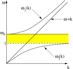
Figure 1: Plot of the linear dispersion relation of Maxwell-Bloch for $\alpha=1$. The two curves are the two solutions $\omega_{1}(k)$ and $\omega_{2}(k)$ of expression (II.30). We have also plotted the plasma frequency $\omega_{0}$ and the free photon line $\omega=k$. Solitons will be generated in the forbidden band gap $]1,\,\omega_{0}]$.

II.3 Initial data.

The above structure of the linear solution shows that it is possible to eliminate the variable $Q(z,t)$ by integrating one equation in the system (II.7). Actually the equation $F_{tt}=-Q_{tt}$ results from the original equation $\nabla\!\times\!{\bf H}=\partial_{t}{\bf D}$ (no current of charges). As the propagation is along $z$, the third component of the curl vanishes, therefore $(\partial_{t}{\bf D})_{z}=0=\partial_{t}(F+Q)$, which allows to express $Q(z,t)$ as $Q(z,t)=-F(z,t)+C(z)$, where the integration constant $C(z)$ remains to be computed. It is naturally determined from the initial conditions. We consider here a situation where the presence of stationary charges produces a permanent electrostatic component $F_{0}(z)$, namely when

$$F(z,t)=\phi(z,t)+F_{0}(z),\quad\phi(z,0)=0.$$ (II.31)

Then the structure (II.19) of the linear solution then implies the following expression for the longitudinal component of the polarization

$$Q(z,t)=\alpha F_{0}(z)-\phi(z,t),$$ (II.32)

where, in the absence of initial electromagnetic irradiation, we have the initial conditions $\{n(z,0)=0,\,\phi(z,0)=0\}$. We now demonstrate that the initial vacuum $\{E=P=0,n=0,\phi=0\}$ and $\{F=F_{0}(z),Q=\alpha F_{0}(z)\}$ is nonlinearly stable as soon as $F_{0}$ is below some threshold.

II.4 Nonlinear stability.

The stability of the initial vacuum is proved for the dynamical variable $\phi(z,t)$ without applied external electromagnetic field $E(z,t)$ (the $x$-component). Replacing expressions (II.31) and (II.32) in the system (II.7), the equation for the electrostatic wave $\phi(z,t)$ becomes

$$\phi_{tt}+\omega_{0}^{2}\phi=\alpha n(\phi+F_{0}).$$ (II.33)

Without applied electromagnetic wave ($E=P=0$), the equation for $n(z,t)$ (the density of population of the excited state) can be integrated taking into account $n(z,0)=0$ and $\phi(z,0)=0$ to give

$$n=-\frac{1}{2}\phi^{2}-\phi F_{0},$$ (II.34)

which, in the evolution for $\phi$, provides the closed equation

$$\phi_{tt}+(\omega_{0}^{2}+\alpha F_{0}^{2})\phi+\frac{\alpha}{2}\phi^{2}(\phi+3F_{0})=0.$$ (II.35)

This is an equation for an anharmonic oscillator whose frequency depends on the parameter $F_{0}(z)$. The solution corresponding to $\phi(z,0)=0$ and $\phi_{t}(z,0)=0$ is obviously $\phi(z,t)=0$, which shows that the initial conditions are consistent. To study the stability, we rewrite the above oscillator as

$$\frac{d}{dt}\left[\frac{1}{2}\phi_{t}^{2}+{\cal E}_{p}\right]=0,\quad{\cal E}_{p}=\frac{1}{2}(\omega_{0}^{2}+\alpha F_{0}^{2})\phi^{2}+\frac{\alpha}{2}F_{0}\,\phi^{3}+\frac{\alpha}{8}\,\phi^{4}.$$

The condition of nonlinear stability is reached when the function ${\cal E}_{p}(\phi)$ has one single minimum in $\phi=0$ (initial condition). The derivative

$$\frac{d{\cal E}_{p}}{d\phi}=\frac{\alpha}{2}\,\phi\left[\phi^{2}+3F_{0}\phi+2(\frac{\omega_{0}^{2}}{\alpha}+F_{0}^{2})\right].$$

vanishes always at $\phi=0$, and there will be no other solutions as soon as $\max_{z}\{F_{0}^{2}\}<8(1+\alpha)/\alpha$ (in our case $\alpha=1$, i.e. $8(1+\alpha)/\alpha=16$). With a single root at $\phi=0$, the potential ${\cal E}_{p}(\phi)$ has a single minimum in $\phi=0$. However, when $\max_{z}\{|F_{0}|\}$ exceeds the threshold value (namely the value 4 with $\alpha=1$), the potential ${\cal E}_{p}(\phi)$ becomes a double well with a local maximum at point $\phi=0$ which is thus unstable (and might be of interest to study). Thus here we shall consider values of $F_{0}$ such that $\max_{z}\{|F_{0}|\}<4$ such that nonlinear stability condition be always satisfied.

Thus we have obtained the initial state reached by the medium submitted to electrical potential (charges), namely to a permanent longitudinal component $F_{0}(z)$ which has been shown to generate a permanent polarization $\alpha F_{0}(z)$ accordingly with (II.32). These data constitute then the initial condition (initial equilibrium ground state) that is now inserted in the model itself.

II.5 Final model.

The model studied from now on eventually reads

$$P_{tt}+P=\alpha(1-n)E,\quad \phi_{tt}+\omega_{0}^{2}\phi=\alpha n(\phi+F_{0}),$$

$$E_{tt}-E_{zz}=-P_{tt},\quad n_{t}=EP_{t}-(\phi+F_{0})\phi_{t},$$ (II.36)

and it is completed by the following initial values (ground state at rest)

$$E(z,0)=0,\quad E_{t}(z,0)=0,\quad P(z,0)=0,\quad P_{t}(z,0)=0,$$

$$\phi(z,0)=0,\quad\phi_{t}(z,0)=0,\quad n(z,0)=0.$$ (II.37)

Two boundary values for the electromagnetic components are now needed, chosen following gap-sol-pra as representing an electromagnetic cavity coupled to the two-level medium by using its stop gap as one side mirror (the cavity works at frequency $\omega$ in the gap). We then assume an open end $z=L$ (vanishing of the magnetic component), therefore we set

$$E(0,t)=a\,\sin(\omega t),\quad E_{z}(L,t)=0,$$ (II.38)

with $\omega\in[1,\,\omega_{0}]$. Last, $F_{0}(z)$ is a given function that results from the presence of charges, (created e.g. with a doped smiconductor, an applied static electric potential, inclusion of metallic nanoparticles,…), and that needs to be evaluated in a given physical context. We present in fig.2 the scheme of principle of the device that corresponds to our problem.

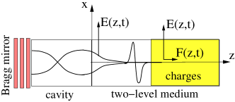
Figure 2: Principle of a situation where the tranverse generated electromagnetic gap soliton would scatter with a permanent longitudinal background $F_{0}(z)$ created by a region with charges (doped smiconductor, applied static electric potential, inclusion of metallic nanoparticles…) where a longitudinal component $F(z,t)$ is generated by nonlinear coupling.

III Numerical simulations

Our purpose is simply here to show that a given function $F_{0}(z)$ acts as a scattering potential on the dynamics of the slow light gap soliton. To that end one needs first to generate the SLGS. It is done by applying the principle of nonlinear supratransmission nst-prl to the MB system as described in gap-sol-pra . There it is proved that the boundary value (II.38) at a frequency in the stop gap, which would linearly produce an evanescent wave in the medium, is actually unstable above a threshold $a_{s}$ given by

$$a_{s}=4\sqrt{2\omega_{0}\,\frac{\omega_{0}-\omega}{\omega_{0}^{2}+3}}$$ (III.1)

where $\omega$ is the driving frequency in the stop gap $[1,\,\omega_{0}]$.

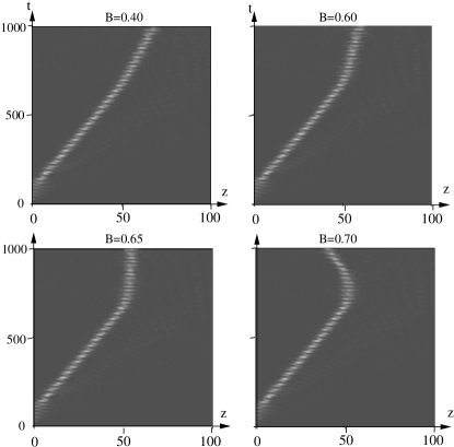
Figure 3: Scattering of the SLGS generated by the boundary (II.38) with $a=0.4$ and $\omega=1.4$ onto the step function $F_{0}(z)$ of (III.2) with $z_{0}=50$ and values of step height $B$ as indicated. These are intensity plots of the energy density flux $-EP/2$ where the brightest regions have value $0.3$.

Let us simply mention that the threshold of nonlinear supratransmission is obtained from the nonlinear Schrödinger limit of MB by assuming a driving frequency close to the gap edge $\omega_{0}$. For instance it is shown in gap-sol-pra this threshold is correct to a high precision close to the edge (typically for $\omega=1.4$ with the edge $\omega_{0}=\sqrt{2}$), precision that decreases to $15\%$ at the frequency $1.2$. But the very question is not the value of the threshold but its existence, source of gap soliton generation. Note that one needs to ensure compatibility of boundary values (II.38) with initial data (II.37) and thus we always start the boundary driving smoothly at $t>0$ such that $E(0,0)=0$. Note also the the stability of the static solution is used to determine a stable vacuum solution inside the region with charges, which is disconnected from the instability of the evanescent wave living in the region without charges.

We display in fig.3 the result of the scattering of a SLGS onto a step potential

$$F_{0}(z)=B\,\theta(z-z_{0}),$$ (III.2)

where $\theta$ is the Heaviside function. We have used as boundary (II.38) the following driving (at frequency $\omega=1.4$)

$$E(0,t)=0.2[\tanh(0.2(t-20))-\tanh(0.5(t-150))]\cos(\omega t),$$ (III.3)

The scattering mechanism will be analyzed in the next section, let us simply mention here that the SLGS is very robust and has been checked to (almost) maintain its amplitude and frequency across the step, the only varying parameter being its velocity. This property will allow us to understand the existence of a threshold step height above which the SLGS is reflected. Below this threshold the SLGS simply slows down to ajust to a different medium.

IV A phenomenological model

IV.1 The NLS model

To describe the gap soliton scattering in a simple and efficient way, we propose here the following model

$$-2i\omega_{0}\psi_{t}+\frac{\omega_{0}^{2}-1}{\omega_{0}^{2}}\,\psi_{zz}+\frac{1}{2}(\omega_{0}^{2}+3)|\psi|^{2}\psi=V(z)\,\psi.$$ (IV.1)

similar to (I.1) and obtained from (A.31) by replacing the action of $\varphi$ by that of an external potential $V(z)$. The related initial-boundary value problem is naturally deduced from relation (A.18) and boundary value (II.38) as

$$\psi(z,0)=0,\quad\psi(0,t)=-i\frac{a}{2}e^{i(\omega-\omega_{0})t}.$$ (IV.2)

This constitutes a phenomenological model where value of the applied potential $V(z)$ is obtained by comparing numerical simulations of the above equation with those of the Maxwell-Bloch system (II.36). We have obtained that

$$V(z)=\frac{1}{2}\,\frac{(\omega_{0}^{2}-1)^{2}}{\omega_{0}^{2}+4}F_{0}(z)^{2},$$ (IV.3)

provides a quite accurate description of the scattering process. The above particular form has been inspired by the nature of the asymptotic expansion in eq.(A.27) with the structure (A.29), especially for the dependence in $F_{0}^{2}$, but the precise expression has been worked out to generate scattering processes similar to those obtained from Maxwell-Bloch. This is illustrated by fig.4 obtained by solving (IV.1) with the above potential and boundary value. Then to compare to the plots of fig.3, we contruct the electromagnetic energy density flux $-EP/2$ which from (A.18) is given by

$$-\frac{1}{2}EP\simeq\frac{1}{2}\left(\psi\,e^{i\omega_{0}t}+\bar{\psi}\,e^{-i\omega_{0}t}\right)^{2}.$$ (IV.4)

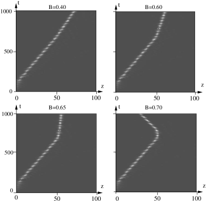
Figure 4: Test of the soliton scattering by use of the NLS model (IV.1) with boundary driving (IV.2) where $a=0.4$ and $\omega=1.4$, and with $V(z)$ given by (IV.3) where $F_{0}(z)=B\,\theta(z-40)$. We have plotted the energy flux density $-EP/2$ given here by (IV.4), which concur with simulations of Maxwell-Bloch of fig.3.

IV.2 Scattering simple rules

The interest of having such a simplified model is to derive explicit formulae for the scattered gap soliton. The NLS equation in a potential has been widely studied, e.g. by use of the inverse spectral theory balak , and especially when the potential is a Dirac delta function representing a local inhomogeneity newell boris holmer , which has also been done for discrete systems peyrard . An interesting application is the study, with a stochastic series of delta functions, of the competition between disorder and nonlinearity kivshar Flach . In our case the step (or barrier) height is not small compared to soliton amplitude ($V_{0}$ is of the order of $max|\psi|^{2}$) and one cannot call to perturbative approach to get analytical description of the scattering process. However, we shall obtain by quite elementary arguments, an expression of the scattered soliton velocity in terms of the incident velocity and the parameters of the medium.

We are interested in potentials $V(z)$ piecewise constant (in regions sufficiently larger than the soliton extension) for which the NLS equation (IV.1) possesses approximate soliton solution in each region, far enough from the discontinuities. The soliton solution of (IV.1) for any $V(z)=V_{0}$ constant is given by

$$\psi_{s}(z,t)=\frac{Ae^{i(\beta z-\mu t)}}{\cosh[\gamma(z-vt)]}$$ (IV.5)

with the following 3 relations linking the 5 coefficients $A$ (amplitude), $\beta$ (wave number), $\mu$ (frequency), $\gamma$ (stiffness) and $v$ (velocity). These are

$$\beta=-\frac{\omega_{0}^{3}}{\omega_{0}^{2}-1}\,v,$$ (IV.6)

$$\gamma^{2}=\frac{A^{2}}{4}(\omega_{0}^{2}+3)\frac{\omega_{0}^{2}}{\omega_{0}^{2}-1},$$ (IV.7)

$$V_{0}=(\gamma^{2}-\beta^{2})\frac{\omega_{0}^{2}-1}{\omega_{0}^{2}}-2\mu\omega_{0}.$$ (IV.8)

One important consequence of the above relations is obtained by elimination of $\beta$ and $\gamma$ and writes

$$v^{2}\frac{\omega_{0}^{4}}{\omega_{0}^{2}-1}=\frac{A^{2}}{4}(\omega_{0}^{2}+3)-2\omega_{0}\mu-V_{0},$$ (IV.9)

which furnishes the soliton velocity from its amplitude $A$ and carrier frequency $\mu$. Note that the solution is a gap soliton which means $\mu>0$.

Now we assume, accordingly with observations of a number of numerical simulations, that the amplitude $A$ and the frequency $\mu$ do not change across a step from a region 1 where $V=0$ to a region 2 where $V=V_{0}$. The soliton is produced in region 1 by the boundary driving and are measured for each numerical experiment as in gap-sol-pra (it is actually easier to measure $v$ and $\mu$ and to deduce $A$). Then the scattering process is understood in a quite simple manner. First formula (IV.9) immediately implies the existence of a particular threshold value of the constant $V_{0}$ for which the velocity in region 2 would vanish and above which this soliton is not a solution. This threshold, called $V_{th}$, is thus obtained by setting $v=0$ in (IV.9) and reads

$$V_{th}=\frac{A^{2}}{4}(\omega_{0}^{2}+3)-2\omega_{0}\mu.$$ (IV.10)

To be clear, this threshold indicates that the NLS equation (IV.1) with $V_{0}>V_{th}$ does not support a soliton solution with the given parameters $A$ and $\mu$. So we expect a reflection on the step of height $V_{0}$ as soon as $V_{0}>V_{th}$.

Below the threshold, the velocity $v^{\prime}$ in region 2 is deduced from (IV.9) and (IV.10) as

$$V_{0}<V_{th}\quad:\quad{v^{\prime}}^{2}=v^{2}-V_{0}\frac{\omega_{0}^{2}-1}{\omega_{0}^{4}},\quad V_{th}=v^{2}\,\frac{\omega_{0}^{4}}{\omega_{0}^{2}-1}.$$ (IV.11)

Here the threshold value $V_{th}$ given in (IV.10) is written in terms of the emitted SLGS velocity $v$ only by computing hereabove the value of $V_{0}$ for which $v^{\prime}=0$.

IV.3 Step potential

In the case of the one-step potential (III.2) we have

$$z>z_{0}\,:\quad V_{0}=\frac{1}{2}\,\frac{(\omega_{0}^{2}-1)^{2}}{\omega_{0}^{2}+4}\,B^{2},$$ (IV.12)

and the velocity $v^{\prime}$ reads from (IV.11)

$${v^{\prime}}^{2}=v^{2}-\frac{B^{2}}{2\omega_{0}^{4}}\,\frac{(\omega_{0}^{2}-1)^{3}}{\omega_{0}^{2}+4}.$$ (IV.13)

As a consequence the threshold amplitude $B_{th}$ of the electrostatic permanent background $F_{0}(z)=B\theta(z-z_{0})$ can be written

$$B_{th}=v\,\omega_{0}^{2}\sqrt{2}\,\frac{(\omega_{0}^{2}+4)^{1/2}}{(\omega_{0}^{2}-1)^{3/2}}.$$ (IV.14)

Figure 5: Soliton velocity $v^{\prime}$ beyond the step location $z_{0}$ in terms of the step height $B$ according to formula (IV.13) plotted as the continuous curve, and measured from simulations of Maxwell-Bloch (points).

We have tested these formulae against numerical simulations of the Maxwell-Bloch system (not simply the NLS model), which is summarized in figure 5. Clearly the small discrepancy between soliton scattering and elementary formula (IV.13) comes on the one side from the assumptions of conservation of shape across the step, on the other side from losses by phonon emission. Note that formula (IV.13) relates the kinetic energy of the soliton in the two media through the potential energy $V_{0}$ of the obstacle. Another interesting aspect of this formula is the fact that the scattered velocity $v^{\prime}$ depends only on the incident velocity $v$, once the step height $V_{0}$ and the coupling constant $\alpha=\omega_{0}^{2}-1$ have been fixed.

Such an expression can be confronted to numerical simulations of Maxwell-Bloch for different values of the coupling parameter $\alpha$ and different incident SLGS velocities $v$ (obtained by varying the driving amplitude).

$$\begin{array}[]{|c|c|c|c|c|c|}\hline\cr\alpha&\omega&a&v&B_{th}&B\\ \hline\cr 1&1.40&0.40&0.088&0.61&0.65\\ \hline\cr 1&1.40&0.42&0.111&0.77&0.72\\ \hline\cr 1&1.40&0.44&0.133&0.92&0.90\\ \hline\cr 1&1.40&0.46&0.154&1.07&1.00\\ \hline\cr 2&1.70&0.60&0.175&0.69&0.70\\ \hline\cr 3&1.95&0.70&0.14&0.45&0.50\\ \hline\cr 4&2.18&0.72&0.15&0.40&0.42\\ \hline\cr 5&2.40&0.70&0.22&0.53&0.54\\ \hline\cr 10&3.25&0.70&0.18&0.34&0.38\\ \hline\cr\end{array}$$ (IV.15)

Some results are presented in table IV.15 where $\alpha$ is the coupling parameter, $a$ and $\omega$ are the chosen driving amplitude and frequency for Maxwell-Bloch as defined in (II.38). Then $v$ is the measured soliton velocity and $B_{th}$ the theoretical threshold for soliton reflection as given by (IV.14). The effective threshold $B$ is then obtained by multiple simulations of Maxwell-Bloch where $F_{0}(z)=B\theta(z-z_{0})$ varying the value of $B$. Such a result shows that the empirical formula (IV.3) for the potential $V(z)$ entering the nonlinear Schrödinger model correctly describes the scattering process within the chosen parameter range.

Conclusion and comments

The main result we wish to emphasize is the demonstration that a slow light gap soliton in a two-level medium can be manipulated by use of a permanent electrostatic background field. Such a property may have interesting applications as it is quite generic and fundamental: a two-level medium constitutes the basic model for any medium submitted to monochromtic radiation close to one transition frequency.

One interesting open problem is the description of the interaction process through the method of perturbative asymptotic expansion. We have indeed discovered that it is the interaction of processes of different orders which is fundamental in the coupling of the electromagnetic field with the electrostatic component. We have not been able to include such interaction in the perturbative asymptotic method as by nature it decouples the different orders. Although the simple nonlinear Schrödinger model (IV.1) describes quite well the SLGS scattering of Maxwell-Bloch, one would appreciate to obtain it by some limit procedure. Actually the NLS equation is a natural limit, it is the expression of the external potential (IV.3) representing the electrostatic permanent background that should be rigorously derived.

One may of course play with different types of potentials, as for instance a barrier of height $B$ and width $D$. In that case at a given height, and a given incident soliton velocity, we observe tunnelling when the width value is below a threshold (e.g. we have obtained tunnelling with parameters of fig.3 at height $B=0.8$ for a width $D<4.5$). This is an interesting problem, obviously related with the delta-function case boris , that will be considered in future studies.

Note finally that the soliton is generated from the boundary driving (II.38) by the nonlinear supratransmission mechanism which is an instability of the evanescent wave leon-instab . As a consequence, the soliton characteristics are quite sensitive to the driving parameters: frequency, amplitude, and shape. The fig.3 has been obtained for the particular boundary value (III.3) and the soliton is generated at a velocity $v=0.88$. A different shape of that driving, keeping same amplitude and frequency, may generate a SLGS with a slightly different velocity. Note that the fundamental question of the relation between soliton characteristics and driving parameters is also an open problem.

Appendix A Perturbative asymptotic analysis

The purpose of this appendix is to provide usefull expressions for the asymptotic model derived from Maxwell-Bloch as in gino but here with non-vanishing permanent fields. Although computations are lengthly, they are standard and we list here only the relevant results.

General expressions

It is actually convenient to consider the full 3-vector case and to reduce it to our particular interest at the very end. The dimensionless Maxwell-Bloch system (II.4) reduced to a propagation in the $z$-direction becomes

$$\partial^{2}_{t}{\bf P}+{\bf P}-\alpha{\bf E}=-\alpha n{\bf E},\quad\partial_{t}n={\bf E}\cdot\partial_{t}{\bf P},$$

$$\left(\partial^{2}_{t}-\sigma\partial^{2}_{z}\right){\bf E}=-\partial^{2}_{t}{\bf P},$$ (A.1)

where the singular matrix $\sigma$ is defined by

$$\sigma=\left(\begin{array}[]{ccc}1&0&0\\ 0&1&0\\ 0&0&0\end{array}\right).$$ (A.2)

The reductive perturbative expansion is a method to extract information about the variations at first order of a formal expansion of the fields in terms of new slow variables, see e.g. the tutorial paper leblond and the refrences therein. We seek slowly varying envelope approximation solutions (SVEA) for a carrier wave at frequency $\omega$ very close to $\omega_{0}$ (and in the gap: $\omega<\omega_{0}$), thus we assume the expansion

$${\bf E}=\sum_{j=1}^{\infty}\epsilon^{j}\sum_{m=-j}^{+j}{\bf E}_{j}^{m}(\xi,\tau)e^{im\omega_{0}t},$$

$${\bf P}=\sum_{j=1}^{\infty}\epsilon^{j}\sum_{m=-j}^{+j}{\bf P}_{j}^{m}(\xi,\tau)e^{im\omega_{0}t},$$ (A.3)

$$n=\sum_{j=1}^{\infty}\epsilon^{j}\sum_{m=-j}^{+j}N_{j}^{m}(\xi,\tau)e^{in\omega_{0}t},$$

in which the reality condition implies

$${\bf E}_{j}^{-m}=\bar{\bf E}_{j}^{m},\quad{\bf P}_{j}^{-m}=\bar{\bf P}_{j}^{m},\quad N_{j}^{-m}=\bar{N}_{j}^{m}.$$ (A.4)

An important issue is to include in the expansion the description of the permanent background $F_{0}(z)$. Then we must assume that ${\bf E}$ and ${\bf P}$ do possess zero-frequency modes, namely that ${\bf E}_{j}^{0}\neq 0$ and ${\bf P}_{j}^{0}\neq 0$. We shall find that these quantities must obey some general constraint but are not governed by an equation (this is the reason why in general they are assumed to vanish) which will allow us to fix them as external data (scattering potential). The slow variables $\xi$ and $\tau$ are here

$$\xi=\epsilon z,\quad\tau=\epsilon^{2}t.$$ (A.5)

Indeed, the natural space variable is usually $\xi=\epsilon(z-vt)$ where $v$ is the group velocity at the frequency of the carrier. Here this frequency is $\omega_{0}$ for which the group velocity vanishes, as implied by the dispersion relation (II.30). Note that this property ensures that the boundary-value problem in the physical space maps effectively to a boundary value problem in the slow space.

Inserting the infinite series expansion (A.3) into the system (A.1) we obtain, after careful (tedious) algebraic computations, the following closed form system at order $\epsilon^{3}$ (remember ${\bf E}_{1}^{-1}=\overline{{\bf E}_{1}^{1}}$)

$$-2i\frac{\omega_{0}}{\alpha}\partial_{\tau}{\bf E}_{1}^{1}+\frac{\sigma}{\omega_{0}^{2}}\partial_{\xi}^{2}{\bf E}_{1}^{1}=-N_{2}^{0}{\bf E}_{1}^{1}+({\bf E}_{1}^{1}\cdot{\bf E}_{1}^{0}){\bf E}_{1}^{0}+\frac{1}{2}({\bf E}_{1}^{1}\cdot{\bf E}_{1}^{1}){\bf E}_{1}^{-1},$$

$$\partial_{\tau}N_{2}^{0}=\partial_{\tau}\left(\frac{\alpha}{2}{\bf E}_{1}^{0}\cdot{\bf E}_{1}^{0}+\frac{\omega_{0}^{2}+1}{\omega_{0}^{2}-1}{\bf E}_{1}^{1}\cdot{\bf E}_{1}^{-1}\right),$$ (A.6)

together with the following constraints on the backgroung field ${\bf E}_{1}^{0}$

$$\left(\begin{array}[]{ccc}\partial_{\xi}^{2}&0&0\\ 0&\partial_{\xi}^{2}&0\\ 0&0&\partial_{\tau}^{2}\end{array}\right){\bf E}_{1}^{0}=0.$$ (A.7)

The principle of the method is then to express all relevant quantities in terms of the solution of the nonlinear evolution (A.6). These are given by

$${\bf E}= \epsilon\left({\bf E}_{1}^{0}+{\bf E}_{1}^{1}e^{i\omega_{0}t}+{\bf E}_{1}^{-1}e^{i\omega_{0}t}\right)+{\cal O}(\epsilon^{2})$$ (A.8)

$${\bf P}= \epsilon\left(\alpha{\bf E}_{1}^{0}-{\bf E}_{1}^{1}e^{i\omega_{0}t}-{\bf E}_{1}^{-1}e^{-i\omega_{0}t}\right)+{\cal O}(\epsilon^{2})$$ (A.9)

$$n= \epsilon^{2}(N_{2}^{0}-{\bf E}_{1}^{1}\cdot{\bf E}_{1}^{0}e^{i\omega_{0}t}-\frac{1}{2}{\bf E}_{1}^{1}\cdot{\bf E}_{1}^{1}e^{2i\omega_{0}t}-{\bf E}_{1}^{-1}\cdot{\bf E}_{1}^{0}e^{-i\omega_{0}t}$$

$$-\frac{1}{2}{\bf E}_{1}^{-1}\cdot{\bf E}_{-1}^{1}e^{-2i\omega_{0}t})+{\cal O}(\epsilon^{3}),$$ (A.10)

where ${\bf E}_{1}^{1}$ and $N_{2}^{0}$ are given in equations (A.6). The structure of the external datum ${\bf E}_{1}^{0}$ resulting from the constraint (A.7) reads

$${\bf E}_{1}^{0}=\left(\begin{array}[]{c}E_{1x}^{0}(\tau)\\ E_{1y}^{0}(\tau)\\ E_{1z}^{0}(\xi)\end{array}\right).$$ (A.11)

where the dependences can be arbitrarily fixed.

Electrostatic potential

By inverse scaling we may come back to the original physical variables $z$ and $t$, and we restrict our study to the case (II.6) where the longitudinal component $F(z,t)=\phi(z,t)+F_{0}(z)$. Rewriting then expressions (A.8)-(A.10) in physical variables, we get at first order (namely $\epsilon$ for ${\bf E}$ and ${\bf P}$, $\epsilon^{2}$ for $n$)

$${\bf E}=\left(\begin{array}[]{c}0\\ 0\\ F_{0}(z)\end{array}\right)+\left[\left(\begin{array}[]{c}\psi(z,t)\\ 0\\ \varphi(z,t)\end{array}\right)e^{i\omega_{0}t}+c.c.\right],$$ (A.18)

$${\bf P}=\left(\begin{array}[]{c}0\\ 0\\ \alpha F_{0}(z)\end{array}\right)-\left[\left(\begin{array}[]{c}\psi(z,t)\\ 0\\ \varphi(z,t)\end{array}\right)e^{i\omega_{0}t}+c.c.\right],$$ (A.25)

$$n=\nu-\left[F_{0}\varphi\,e^{i\omega_{0}t}+\frac{1}{2}(\psi^{2}+\varphi^{2})\,e^{2i\omega_{0}t}+c.c.\right]$$ (A.26)

where we rename $(E_{1}^{1})_{x}=\psi$, $(E_{1}^{1})_{z}=\varphi$ and $N_{2}^{0}=\nu$. The corresponding evolutions (A.6) eventually read

$$-2i\omega_{0}\psi_{t}+\frac{\omega_{0}^{2}-1}{\omega_{0}^{2}}\,\psi_{zz}=-\alpha\nu\psi+\frac{\alpha}{2}(\psi^{2}+\varphi^{2})\bar{\psi},$$ (A.27)

$$-2i\omega_{0}\varphi_{t}-\alpha(F_{0})^{2}\varphi=-\alpha\nu\varphi+\frac{\alpha}{2}(\psi^{2}+\varphi^{2})\bar{\varphi},$$ (A.28)

$$\nu_{t}=\partial_{t}\left(\frac{\alpha}{2}(F_{0})^{2}+\frac{\omega_{0}^{2}+1}{\omega_{0}^{2}-1}(|\psi|^{2}+|\varphi|^{2})\right).$$ (A.29)

Thanks to the initial data (II.37), namely here to $\psi(z,0)=0$, $\varphi(z,0)=0$ and $\nu(z,0)=0$, we may integrate now the evolution of $\nu$ to get

$$\nu=\frac{\omega_{0}^{2}+1}{\omega_{0}^{2}-1}(|\psi|^{2}+|\varphi|^{2}).$$ (A.30)

Inserted in the equations for $\psi$ and $\varphi$ it gives the final NLS-like system

$$-2i\omega_{0}\psi_{t}+ \frac{\omega_{0}^{2}-1}{\omega_{0}^{2}}\,\psi_{zz}+\frac{1}{2}(\omega_{0}^{2}+3)|\psi|^{2}\psi=$$

$$\frac{1}{2}(\omega_{0}^{2}-1)\varphi^{2}\bar{\psi}-(\omega_{0}^{2}+1)|\varphi|^{2}\psi,$$ (A.31)

$$-2i\omega_{0}\varphi_{t}- \alpha(F_{0})^{2}\varphi+\frac{1}{2}(\omega_{0}^{2}+3)|\varphi|^{2}\varphi=$$

$$\frac{1}{2}(\omega_{0}^{2}-1)\psi^{2}\bar{\varphi}-(\omega_{0}^{2}+1)|\psi|^{2}\varphi.$$ (A.32)

The equation (A.31) is a nonlinear Schrödinger equation for $\psi$ (envelope of the tranverse electromagnetic component) in some external potential created by $\varphi$, the envelope of the plasma wave. The applied permanent background $F_{0}(z)$ does not act directly on $\psi$ but through the plasma wave $\varphi$ according to the dynamical equation (A.32).

The above asymptotic analysis has allowed to demonstrate that the elimination of the variable $Q(z,t)$ by equations (II.31) and (II.32), namely by comes naturally as the first order solution. Then the initial condition $\phi(z,0)=n(z,0)=0$ was shown to be stable in the absence of applied electromagnetic transverse component. By means of (A.18), such a set of initial data maps to $\varphi(z,0)=0$. The problem is that the evolution (A.32) has the unique solution $\varphi(z,t)=0$ for initial data $\varphi(z,0)=0$ and $\varphi_{t}(z,0)=0$ (representing an initial equilibrium state). Thus we are not able to use the system of NLS-like equations (A.31)(A.32) to describe the gap soliton scattering with purely vanishing initial data.

This comes from the fact that the scattering process in Maxwell-Bloch is initiated at higher orders by nonlinear coupling. Indeed, considering the MB system (II.36) with initial-boundary value problem (II.37)(II.38), it is clear that the interaction of $E$ (electromagnetic component) with the permanent electrostatic background $F_{0}(z)$ works with the birth of the plasma wave $\phi$. And $\phi$ grows on an initial vacuum by mediation of the normalized density $n$ of population of the excited level, which is an effect of second order (see the time evolution of $n(z,t)$). But the method of multiscale asymptotic series separates the orders as indeed, at each order $\epsilon^{n}$ an equation is obtained (independent of $\epsilon$). We thus cannot expect the method to describe correctly such a situation.

We have pursued the series to order $\epsilon^{5}$ to check that indeed no source term appear. As expected from the method, we got a linear system for the next order expansion with the variable coefficients $\varphi$ and $\psi$, given from the preceding order. This confirms that the method does not allow feedback interaction of higher orders to the fundamental one $\{\psi,\varphi\}$.

Aknowledgements. This work has been done as part of the programm GDR 3073 Nonlinear Photonics and Microstructured Media.

References

- (1) P. Yeh (2005) Optical waves in layered media, Wiley-Interscience (Hoboken, New Jersey)
- (2) Y.S. Kivshar, G.P. Agrawall, Optical Solitons: From Fibers to Photonic Crystals, Academic Press, San Diego, CA (2003)
- (3) O. Morsch, J. H. M ller, M. Cristiani, D. Ciampini, E. Arimondo, Phys Rev Lett 87 (2001) 140402
- (4) D.R. Meacher, Contemp. Phys. 39 (1998) 329
- (5) P. Yeh (1993) Introduction to photorefractive nonlinear optics, Wiley (New-York).
- (6) V.M. Fain and Ya.I. Khanin (1969) Quantum Electronics, Pergamon (Oxford, UK)
- (7) L.C. Allen, J.H. Eberly (1987) Optical Resonance and Two-Level Atoms (Dover, New York)
- (8) V.S. Butylkin, A.E. Kaplan, Yu.G. Khronopulo and E.I. Yakubovich (1989) Resonant nonlinear interactions of light with matter, Springer (Heidelberg, Germany)
- (9) R.H. Pantell, H.E. Puthoff (1969) Fundamentals of Quantum Electronics (Wiley, New York)
- (10) S.L. Mac Call, E.L. Hahn, Phys Rev 183 (1969)457
- (11) A.I. Maimistov, A.M. Basharov, S.O. Elyutin, Yu. M. Sklyarov, Phys Reports 191 (1990) 1-108
- (12) G.L. Lamb Jr, Phys Rev A 9 (1974) 422
- (13) M.J. Ablowitz, D.J. Kaup, A.C. Newell, J Math Phys 15 (1974) 1852
- (14) J.D. Gibbon, P.J. Caudrey, R.K. Bullough, J.C. Eilbeck, Lett Nuovo Cimento 8 (1973) 775
- (15) I.R. Gabitov, V.E. Zakharov, A.V. Mikhailov, Theor Math Phys 63 (1985) 328
- (16) M. Agrotis, N.M. Ercolani, S.A. Glasgow, J.V. Moloney, Physica D 138 (2000) 134
- (17) F. Hynne, R.K. Bullough, Phil Trans R Soc London A 330 (1990) 253
- (18) S.V. Branis, O. Martin, J.L. Birman, Phys Rev Lett 65 (1990) 2638
- (19) B.I. Mantsyzov, R.N. Kuz’min, Sov Phys JETP 64 (1986) 37; B.I. Mantsyzov, Phys Rev A51 (1995) 4939; B.I. Mantsyzov, R.A. Silnikov, J Opt Soc Amer B19 (2002) 2203; B.I. Mantsyzov, JETP lett 82 (2005) 253
- (20) W. Xiao, J. Zhou, J. Prineas, Optics Express 11 (2003) 3277
- (21) I.V. Mel’nikov, J.S. Aitchison, Appl Phys Lett 87 (2005) 201111
- (22) A.E. Kozhekin, G. Kurizki, Phys Rev Lett 74 (1995) 5020
- (23) A.E. Kozhekin, G. Kurizki, B. Malomed, Phys Rev Lett 81 (1998) 3647
- (24) N. Aközbek, S. John, Phys Rev E 58 (1998) 3876
- (25) H. Raether (1988) Surface plasmons on smooth and rough surfaces and on gratings, Springer (Berlin)
- (26) I.R. Gabitov, A.O. Korotkevitch, A.I. Maimistov, J.B. McMahon, Appl Phys A: Materials Science & Processing 89 (2007) 277
- (27) F. Ginovart, J. Leon, J Phys A: Math Gen 27 (1994) 3955
- (28) R. Khomeriki, J. Leon, Phys Rev Lett 99 (2007) 183601
- (29) J. Leon, Phys Rev A 75 (2007) 06811
- (30) F. Geniet, J. Leon, Phys Rev Lett 89 (2002) 134102
- (31) H. Leblond, J Phys B: At Mol Opt Phys 41 (2008) 043001
- (32) R. Balakrishnan, Phys Rev A 32 (1985) 1144
- (33) A.C. Newel, J Math Phys 19 (1978) 1126
- (34) X.D. Cao, B.A Malomed, Phys Lett A 206 (1995) 177
- (35) J. Holmer, J. Marzuola, M. Zworski, Comm Math Phys 274 (2007) 187
- (36) K. Forinash, M. Peyrard, B. Malomed, Phys Rev E 49 (1994) 3400
- (37) Yu.S. Kivshar, S.A. Gredeskul, A. Sanchez, L. Vazquez, Phys Rev Lett 64 (1990) 1693
- (38) R.A. Vicencio, S. Flach, Control of wavepacket spreading in nonlinear finite disordered lattices, http://arxiv.org/abs/0809.2115
- (39) J. Leon, Phys Lett A 319 (2003) 130