Partial Correlation Estimation by Joint Sparse Regression Models

Abstract

In this paper, we propose a computationally efficient approach —space(Sparse PArtial Correlation Estimation)— for selecting non-zero partial correlations under the high-dimension-low-sample-size setting. This method assumes the overall sparsity of the partial correlation matrix and employs sparse regression techniques for model fitting. We illustrate the performance of space by extensive simulation studies. It is shown that space performs well in both non-zero partial correlation selection and the identification of hub variables, and also outperforms two existing methods. We then apply space to a microarray breast cancer data set and identify a set of hub genes which may provide important insights on genetic regulatory networks. Finally, we prove that, under a set of suitable assumptions, the proposed procedure is asymptotically consistent in terms of model selection and parameter estimation.

key words: concentration network, high-dimension-low-sample-size, lasso, shooting, genetic regulatory network

1 INTRODUCTION

There has been a large amount of literature on covariance selection: the identification and estimation of non-zero entries in the inverse covariance matrix (a.k.a. concentration matrix or precision matrix) starting from the seminal paper by Dempster1972. Covariance selection is very useful in elucidating associations among a set of random variables, as it is well known that non-zero entries of the concentration matrix correspond to non-zero partial correlations. Moreover, under Gaussianity, non-zero entries of the concentration matrix imply conditional dependency between corresponding variable pairs conditional on the rest of the variables edward. Traditional methods does not work unless the sample size ($n$) is larger than the number of variables ($p$) Whittaker1990,edward. Recently, a number of methods have been introduced to perform covariance selection for data sets with $p>n$, for example, see meinshausen, Yuan, Li, SchaferStrimmer07.

In this paper, we propose a novel approach using sparse regression techniques for covariance selection. Our work is partly motivated by the construction of genetic regulatory networks (GRN) based on high dimensional gene expression data. Denote the expression levels of $p$ genes as $y_{1},\cdots,y_{p}$. A concentration network is defined as an undirected graph, in which the $p$ vertices represent the $p$ genes and an edge connects gene $i$ and gene $j$ if and only if the partial correlation $\rho^{ij}$ between $y_{i}$ and $y_{j}$ is non-zero. Note that, under the assumption that $y_{1},\cdots,y_{p}$ are jointly normal, the partial correlation $\rho^{ij}$ equals to ${\rm Corr}(y_{i},y_{j}|y_{-(i,j)})$, where $y_{-(i,j)}=\{y_{k}:1\leq k\not=i,j\leq p\}$. Therefore, $\rho^{ij}$ being nonzero is equivalent to $y_{i}$ and $y_{j}$ being conditionally dependent given all other variables $y_{-(i,j)}$. The proposed method is specifically designed for the high-dimension-low-sample-size scenario. It relies on the assumption that the partial correlation matrix is sparse (under normality assumption, this means that most variable pairs are conditionally independent), which is reasonable for many real life problems. For instance, it has been shown that most genetic networks are intrinsically sparse gardner,jeong,tegner. The proposed method is also particularly powerful in the identification of hubs: vertices (variables) that are connected to (have nonzero partial correlations with) many other vertices (variables). The existence of hubs is a well known phenomenon for many large networks, such as the internet, citation networks, and protein interaction networks newman. In particular, it is widely believed that genetic pathways consist of many genes with few interactions and a few hub genes with many interactions barabasi.

Another contribution of this paper is to propose a novel algorithm active-shooting for solving penalized optimization problems such as lasso Ti96. This algorithm is computationally more efficient than the original shooting algorithm, which was first proposed by Fu1998shooting and then extended by many others including Genkin07 and Tibshirani2007PathCO. It enables us to implement the proposed procedure efficiently, such that we can conduct extensive simulation studies involving $\sim 1000$ variables and hundreds of samples. To our knowledge, this is the first set of intensive simulation studies for covariance selection with such high dimensions.

A few methods have also been proposed recently to perform covariance selection in the context of $p\gg n$. Similar to the method proposed in this paper, they all assume sparsity of the partial correlation matrix. meinshausen introduced a variable-by-variable approach for neighborhood selection via the lasso regression. They proved that neighborhoods can be consistently selected under a set of suitable assumptions. However, as regression models are fitted for each variable separately, this method has two major limitations. First, it does not take into account the intrinsic symmetry of the problem (i.e., $\rho^{ij}=\rho^{ji}$). This could result in loss of efficiency, as well as contradictory neighborhoods. Secondly, if the same penalty parameter is used for all $p$ lasso regressions as suggested by their paper, more or less equal effort is placed on building each neighborhood. This apparently is not the most efficient way to address the problem, unless the degree distribution of the network is nearly uniform. However, most real life networks have skewed degree distributions, such as the power-law networks. As observed by SchaferStrimmer07, the neighborhood selection approach limits the number of edges connecting to each node. Therefore, it is not very effective in hub detection. On the contrary, the proposed method is based on a joint sparse regression model, which simultaneously performs neighborhood selection for all variables. It also preserves the symmetry of the problem and thus utilizes data more efficiently. We show by intensive simulation studies that our method performs better in both model selection and hub identification. Moreover, as a joint model is used, it is easier to incorporate prior knowledge such as network topology into the model. This is discussed in Section 2.1.

Besides the regression approach mentioned above, another class of methods employ the maximum likelihood framework. Yuan proposed a penalized maximum likelihood approach which performs model selection and estimation simultaneously and ensures the positive definiteness of the estimated concentration matrix. However, their algorithm can not handle high dimensional data. The largest dimension considered by them is $p=10$ in simulation and $p=5$ in real data. TiSparse07 proposed an efficient algorithm glasso to implement this method, such that it can be applied to problems with high dimensions. We show by simulation studies that, the proposed method performs better than glasso in both model selection and hub identification. rothman08 proposed another algorithm to implement the method of Yuan. The computational cost is on the same order of glasso, but in general not as efficient as glasso. Li introduced a threshold gradient descent (TGD) regularization procedure. SchaferStrimmer07 proposed a shrinkage covariance estimation procedure to overcome the ill-conditioned problem of sample covariance matrix when $p>n$. There are also a large class of methods covering the situation where variables have a natural ordering, e.g., longitudinal data, time series, spatial data, or spectroscopy. See wu03, BickelLevina08, huang06 and levina_zhu06, which are all based on the modified Cholesky decomposition of the concentration matrix. In this paper, we, however, focus on the general case where an ordering of the variables is not available.

The rest of the paper is organized as follows. In Section 2, we describe the joint sparse regression model, its implementation and the active-shooting algorithm. In Section 3, the performance of the proposed method is illustrated through simulation studies and compared with that of the neighborhood selection approach and the likelihood based approach glasso. In Section 4, the proposed method is applied to a microarray expression data set of $n=244$ breast cancer tumor samples and $p=1217$ genes. In Section 5, we study the asymptotic properties of this procedure. A summary of the main results are given in Section 6. Technique details are provided in the Supplemental Material.

2 METHOD

2.1 Model

In this section, we describe a novel method for detecting pairs of variables having nonzero partial correlations among a large number of random variables based on i.i.d. samples. Suppose that, $(y_{1},\cdots,y_{p})^{T}$ has a joint distribution with mean $0$ and covariance $\mathbf{\Sigma}$, where $\mathbf{\Sigma}$ is a $p$ by $p$ positive definite matrix. Denote the partial correlation between $y_{i}$ and $y_{j}$ by $\rho^{ij}$ ($1\leq i<j\leq p$). It is defined as ${\rm Corr}(\epsilon_{i},\epsilon_{j})$, where $\epsilon_{i}$ and $\epsilon_{j}$ are the prediction errors of the best linear predictors of $y_{i}$ and $y_{j}$ based on $y_{-(i,j)}=\{y_{k}:1\leq k\not=i,j\leq p\}$, respectively. Denote the concentration matrix $\mathbf{\Sigma}^{-1}$ by $(\sigma^{ij})_{p\times p}$. It is known that, $\rho^{ij}=-\frac{\sigma^{ij}}{\sqrt{\sigma^{ii}\sigma^{jj}}}$. Let $y_{-i}:=\{y_{k}:1\leq k\not=i\leq p\}$. The following well-known result (Lemma 1) relates the estimation of partial correlations to a regression problem.

Lemma 1

: For $1\leq i\leq p$, $y_{i}$ is expressed as $y_{i}=\sum_{j\not=i}\beta_{ij}y_{j}+\epsilon_{i}$, such that $\epsilon_{i}$ is uncorrelated with $y_{-i}$ if and only if $\beta_{ij}=-\frac{\sigma^{ij}}{\sigma^{ii}}=\rho^{ij}\sqrt{\frac{\sigma^{jj}}{\sigma^{ii}}}$. Moreover, for such defined $\beta_{ij}$, ${\rm Var}(\epsilon_{i})=\frac{1}{\sigma^{ii}},{\rm Cov}(\epsilon_{i},\epsilon_{j})=\frac{\sigma^{ij}}{\sigma^{ii}\sigma^{jj}}$.

Note that, under the normality assumption, $\rho^{ij}={\rm Corr}(y_{i},y_{j}|y_{-(i,j)})$ and in Lemma 1, we can replace “uncorrelated” with “independent”. Since $\rho^{ij}={\rm sign}(\beta_{ij})\sqrt{\beta_{ij}\beta_{ji}}$, the search for non-zero partial correlations can be viewed as a model selection problem under the regression setting. In this paper, we are mainly interested in the case where the dimension $p$ is larger than the sample size $n$. This is a typical scenario for many real life problems. For example, high throughput genomic experiments usually result in data sets of thousands of genes for tens or at most hundreds of samples. However, many high-dimensional problems are intrinsically sparse. In the case of genetic regulatory networks, it is widely believed that most gene pairs are not directly interacting with each other. Sparsity suggests that even if the number of variables is much larger than the sample size, the effective dimensionality of the problem might still be within a tractable range. Therefore, we propose to employ sparse regression techniques by imposing the $\ell_{1}$ penalty on a suitable loss function to tackle the high-dimension-low-sample-size problem.

Suppose $\mathbf{Y}^{k}=(y^{k}_{1},\cdots,y^{k}_{p})^{T}$ are i.i.d. observations from $(0,\mathbf{\Sigma})$, for $k=1,\cdots,n$. Denote the sample of the $i$th variable as $\mathbf{Y}_{i}=(y^{1}_{i},\cdots,y^{n}_{i})^{T}$. Based on Lemma 1, we propose the following joint loss function

$$L_{n}(\mathbf{\theta},\mathbf{\sigma},\mathbf{Y}) = \frac{1}{2}\Bigl{(}\sum_{i=1}^{p}w_{i}||\mathbf{Y}_{i}-\sum_{j\not=i}\beta_{ij}\mathbf{Y}_{j}||^{2}\Bigr{)}$$ (1)

$$= \frac{1}{2}\Bigl{(}\sum_{i=1}^{p}w_{i}||\mathbf{Y}_{i}-\sum_{j\not=i}\rho^{ij}\sqrt{\frac{\sigma^{jj}}{\sigma^{ii}}}\mathbf{Y}_{j}||^{2}\Bigr{)},$$

where $\mathbf{\theta}=(\rho^{12},\cdots,\rho^{(p-1)p})^{T}$, $\mathbf{\sigma}=\{\sigma^{ii}\}_{i=1}^{p}$; $\mathbf{Y}=\{\mathbf{Y}^{k}\}_{k=1}^{n}$; and $w=\{w_{i}\}_{i=1}^{p}$ are nonnegative weights. For example, we can choose $w_{i}=1/{\rm Var}(\epsilon_{i})=\sigma^{ii}$ to weigh individual regressions in the joint loss function according to their residual variances, as is done in regression with heteroscedastic noise. We propose to estimate the partial correlations $\mathbf{\theta}$ by minimizing a penalized loss function

$$\mathcal{L}_{n}(\mathbf{\theta},\mathbf{\sigma},\mathbf{Y})=L_{n}(\mathbf{\theta},\mathbf{\sigma},\mathbf{Y})+\mathcal{J}(\mathbf{\theta}),$$ (2)

where the penalty term $\mathcal{J}(\mathbf{\theta})$ controls the overall sparsity of the final estimation of $\theta$. In this paper, we focus on the $\ell_{1}$ penalty Ti96:

$${\mathcal{J}}(\mathbf{\theta})=\lambda||\mathbf{\theta}||_{1}=\lambda\sum_{1\leq i<j\leq p}|\rho^{ij}|.$$ (3)

The proposed joint method is referred to as space (Sparse PArtial Correlation Estimation) hereafter. It is related to the neighborhood selection approach by meinshausen (referred to as MB hereafter), where a lasso regression is performed separately for each variable on the rest of the variables. However, space has several important advantages.

1. In space, sparsity is utilized for the partial correlations $\theta$ as a whole view. However, in the neighborhood selection approach, sparsity is imposed on each neighborhood. The former treatment is more natural and utilizes the data more efficiently, especially for networks with hubs. A prominent example is the genetic regulatory network, where master regulators are believed to exist and are of great interest.

2. According to Lemma 1, $\beta_{ij}$ and $\beta_{ji}$ have the same sign. The proposed method assures this sign consistency as it estimates $\{\rho^{ij}\}$ directly. However, when fitting $p$ separate (lasso) regressions, it is possible that ${\rm sign}(\widehat{\beta}_{ij})$ is different from ${\rm sign}(\widehat{\beta}_{ji})$, which may lead to contradictory neighborhoods.

3. Furthermore, the utility of the symmetric nature of the problem allows us to reduce the number of unknown parameters in the model by almost half ($p(p+1)/2$ for space vs. $(p-1)^{2}$ for MB), and thus improves the efficiency.

4. Finally, prior knowledge of the network structure are often available. The joint model is more flexible in incorporating such prior knowledge. For example, we may assign different weights $w_{i}$ to different nodes according to their “importance”. We have already discussed the residual variance weights, where $w_{i}=\sigma^{ii}$. We can also consider the weight that is proportional to the (estimated) degree of each variable, i.e., the estimated number of edges connecting with each node in the network. This would result in a preferential attachment effect which explains the cumulative advantage phenomena observed in many real life networks including GRNs barabasiAlbert.

These advantages help enhance the performance of space. As illustrated by the simulation study in Section 3, the proposed joint method performs better than the neighborhood selection approach in both non-zero partial correlation selection and hub detection.

As compared to the penalized maximum likelihood approach glasso TiSparse07, the simulation study in Section 3 shows that space also outperforms glasso in both edge detection and hub identification under all settings that we have considered. In addition, space has the following advantages.

1. The complexity of glasso is $O(p^{3})$, while as discussed in Section 2.2, the space algorithm has the complexity of $\min(O(np^{2}),O(p^{3}))$, which is much faster than the algorithm of Yuan and in general should also be faster than glasso when $n<p$, which is the case in many real studies.

2. As discussed in Section 6, space allows for trivial generalizations to other penalties of the form of $|\rho^{ij}|^{q}$ rather than simply $|\rho^{ij}|$, which includes ridge and bridge [FuFu1998] or other more complicated penalties like SCAD [Fan and LiFan and Li2001]. The glasso algorithm, on the other hand, is tied to the lasso formulation and cannot be extended to other penalties in a natural manner.

3. In Section 5, we prove that our method consistently identifies the correct network neighborhood when both $n$ and $p$ go to $\infty$. As far as we are aware, no such theoretical results have been developed for the penalized maximum likelihood approach.

Note that, in the penalized loss function (2), $\mathbf{\sigma}$ needs to be specified. We propose to estimate $\mathbf{\theta}$ and $\mathbf{\sigma}$ by a two-step iterative procedure. Given an initial estimate $\mathbf{\sigma}^{(0)}$ of $\mathbf{\sigma}$, $\mathbf{\theta}$ is estimated by minimizing the penalized loss function (2), whose implementation is discussed in Section 2.2. Then given the current estimates $\mathbf{\theta}^{(c)}$ and $\mathbf{\sigma}^{(c)}$, $\mathbf{\sigma}$ is updated based on Lemma 1: $1/\widehat{\sigma}^{ii}=\frac{1}{n}||\mathbf{Y}_{i}-\sum_{j\not=i}\widehat{\beta}^{(c)}_{ij}\mathbf{Y}_{j}||^{2}$, where $\widehat{\beta}^{(c)}_{ij}=(\rho^{ij})^{(c)}\sqrt{\frac{(\sigma^{jj})^{(c)}}{(\sigma^{ii})^{(c)}}}$. We then iterate between these two steps until convergence. Since $1/\sigma^{ii}\leq{\rm Var}(y_{i})=\sigma_{ii}$, we can use $1/\widehat{\sigma}_{ii}$ as the initial estimate of $\sigma^{ii}$, where $\widehat{\sigma}_{ii}=\frac{1}{n-1}\sum_{k=1}^{n}(y^{k}_{i}-\bar{y}_{i})^{2}$ is the sample variance of $y_{i}$. Our simulation study shows that, it usually takes no more than three iterations for this procedure to stabilize.

2.2 Implementation

In this section, we discuss the implementation of the space procedure: that is, minimizing (2) under the $\ell_{1}$ penalty (3). We first re-formulate the problem, such that the loss function (1) corresponds to the $\ell_{2}$ loss of a “regression problem.” We then use the active-shooting algorithm proposed in Section 2.3 to solve this lasso regression problem efficiently.

Given $\mathbf{\sigma}$ and positive weights $w$, let $\mathcal{Y}=(\tilde{\mathbf{Y}}_{1}^{T},...,\tilde{\mathbf{Y}}_{p}^{T})^{T}$ be a $np\times 1$ column vector, where $\tilde{\mathbf{Y}}_{i}=\sqrt{w_{i}}\mathbf{Y}_{i}$ ($i=1,\cdots,p$); and let $\mathcal{X}=(\tilde{\mathcal{X}}_{(1,2)},\cdots,\tilde{\mathcal{X}}_{(p-1,p)})$ be a $np$ by $p(p-1)/2$ matrix, with

$$\begin{array}[]{ccccc}\tilde{\mathcal{X}}_{(i,j)}=(0,...,0,&\sqrt{\frac{\tilde{\sigma}^{jj}}{\tilde{\sigma}^{ii}}}\tilde{\mathbf{Y}}_{j}^{T},&0,...,0,&\sqrt{\frac{\tilde{\sigma}^{ii}}{\tilde{\sigma}^{jj}}}\tilde{\mathbf{Y}}_{i}^{T},&0,...,0)^{T}\\ &\uparrow&&\uparrow&\\ &i^{th}\textrm{block}&&j^{th}\textrm{block}&\end{array},$$

where $\tilde{\sigma}^{ii}=\sigma^{ii}/w_{i}$ ($i=1,\cdots,p$). Then it is easy to see that the loss function (1) equals to $\frac{1}{2}||\mathcal{Y}-\mathcal{X}\mathbf{\theta}||_{2}^{2}$, and the corresponding $\ell_{1}$ minimization problem is equivalent to: $\min_{\mathbf{\theta}}\frac{1}{2}||\mathcal{Y}-\mathcal{X}\mathbf{\theta}||_{2}^{2}+\lambda||\mathbf{\theta}||_{1}$. Note that, the current dimension $\tilde{n}=np$ and $\tilde{p}=p(p-1)/2$ are of a much higher order than the original $n$ and $p$. This could cause serious computational problems. Fortunately, $\mathcal{X}$ is a block matrix with many zero blocks. Thus, algorithms for lasso regressions can be efficiently implemented by taking into consideration this structure (see the Supplemental Material for the detailed implementation). To further decrease the computational cost, we develop a new algorithm active-shooting (Section 2.3) for the space model fitting. Active-shooting is a modification of the shooting algorithm, which was first proposed by Fu1998shooting and then extended by many others including Genkin07 and Tibshirani2007PathCO. Active-shooting exploits the sparse nature of sparse penalization problems in a more efficient way, and is therefore computationally much faster. This is crucial for applying space for large $p$ and/or $n$. It can be shown that the computational cost of space is $\min(O(np^{2}),O(p^{3}))$, which is the same as applying $p$ individual lasso regressions as in the neighborhood selection approach. We want to point out that, the proposed method can also be implemented by lars lars. However, unless the exact whole solution path is needed, compared with shooting type algorithms, lars is computationally less appealing Tibshirani2007PathCO. (Remark by the authors: after this paper was submitted, recently the active-shooting idea was also proposed by Friedman08.)

Finally, note that the concentration matrix should be positive definite. In principle, the proposed method (or more generally, the regression based methods) does not guarantee the positive definiteness of the resulting estimator, while the likelihood based method by Yuan and TiSparse07 assures the positive definiteness. While admitting that this is one limitation of the proposed method, we argue that, since we are more interested in model selection than parameter estimation in this paper, we are less concerned with this issue. Moreover, in Section 5, we show that the proposed estimator is consistent under a set of suitable assumptions. Therefore, it is asymptotically positive definite. Indeed, the space estimators are rarely non-positive-definite under the high dimensional sparse settings that we are interested in. More discussions on this issue can be found in Section 3.

2.3 Active Shooting

In this section, we propose a computationally very efficient algorithm active-shooting for solving lasso regression problems. Active-shooting is motivated by the shooting algorithm Fu1998shooting, which solves the lasso regression by updating each coordinate iteratively until convergence. Shooting is computationally very competitive compared with the well known lars procedure lars. Suppose that we want to minimize an $\ell_{1}$ penalized loss function with respect to $\beta$

$$f(\beta)=\frac{1}{2}||\mathbf{Y}-\mathbf{X}\mathbf{\beta}||_{2}^{2}+\gamma\sum_{j}|\beta_{j}|,$$

where $\mathbf{Y}=(y_{1},\cdots,y_{n})^{T}$, $\mathbf{X}=(x_{ij})_{n\times p}=(\mathbf{X}_{1}:\cdots:\mathbf{X}_{p})$ and $\mathbf{\beta}=(\beta_{1},\cdots,\beta_{p})^{T}$. The shooting algorithm proceeds as follows:

• Initial step: for $j=1,\cdots,p,$

  $$\begin{array}[]{rl}\beta_{j}^{(0)}&=~{}\textrm{arg}\min_{\beta_{j}}\{\frac{1}{2}||\mathbf{Y}-\beta_{j}\mathbf{X}_{j}||^{2}+\gamma|\beta_{j}|\}\\ &=~{}\textrm{sign}(\mathbf{Y}^{T}\mathbf{X}_{j})\frac{(|\mathbf{Y}^{T}\mathbf{X}_{j}|-\gamma)_{+}}{\mathbf{X}_{j}^{T}\mathbf{X}_{j}},\end{array}$$ (4)

  where $(x)_{+}=xI_{(x>0)}$.

• For $j=1,...,p$, update $\beta^{(old)}\longrightarrow\beta^{(new)}:$

  $$\begin{array}[]{rl}\beta^{(new)}_{i}&=~{}\beta^{(old)}_{i},i\neq j;\\ \beta^{(new)}_{j}&=~{}\textrm{arg}\min_{\beta_{j}}{\frac{1}{2}\left\|\mathbf{Y}-\sum_{i\neq j}\beta_{i}^{(old)}\mathbf{X}_{i}-\beta_{j}\mathbf{X}_{j}\right\|^{2}+\gamma|\beta_{j}|}\\ &=~{}\textrm{sign}\left(\frac{(\mathbf{\epsilon}^{(old)})^{T}\mathbf{X}_{j}}{\mathbf{X}^{T}_{j}\mathbf{X}_{j}}+\beta_{j}^{(old)}\right)\left(\left|\frac{(\mathbf{\epsilon}^{(old)})^{T}\mathbf{X}_{j}}{\mathbf{X}^{T}_{j}\mathbf{X}_{j}}+\beta^{(old)}_{j}\right|-\frac{\gamma}{\mathbf{X}^{T}_{j}\mathbf{X}_{j}}\right)_{+},\end{array}$$ (5)

  where $\mathbf{\epsilon}^{(old)}=\mathbf{Y}-\mathbf{X}\mathbf{\beta}^{(old)}$.

• Repeat step $2$ until convergence.

At each updating step of the shooting algorithm, we define the set of currently non-zero coefficients as the active set. Since under sparse models, the active set should remain small, we propose to first update the coefficients within the active set until convergence is achieved before moving on to update other coefficients. The active-shooting algorithm proceeds as follows:

• Initial step: same as the initial step of shooting.

• Define the current active set $\Lambda=\{k:\hbox{current}~{}\beta_{k}\neq 0\}$.

  • For each $k\in\Lambda$, update $\beta_{k}$ with all other coefficients fixed at the current value as in equation (5);

  • Repeat (2.1) until convergence is achieved on the active set.

• For $j=1$ to $p$, update $\beta_{j}$ with all other coefficients fixed at the current value as in equation (5). If no $\beta_{j}$ changes during this process, return the current $\beta$ as the final estimate. Otherwise, go back to step 2.

Table 1: The numbers of iterations required by the shooting algorithm and the active-shooting algorithm to achieve convergence ($n=100$, $\lambda=2$). “coef. $\#$” is the number of non-zero coefficients

$p$	coef. $\#$	shooting	active-shooting
200	14	29600	4216
500	25	154000	10570
1000	28	291000	17029

The idea of active-shooting is to focus on the set of variables that is more likely to be in the model, and thus it improves the computational efficiency by achieving a faster convergence. We illustrate the improvement of the active-shooting over the shooting algorithm by a small simulation study of the lasso regression (generated in the same way as in Section 5.1 of Tibshirani2007PathCO). The two algorithms result in exact same solutions. However, as can be seen from Table 1, active-shooting takes much fewer iterations to converge (where one iteration is counted whenever an attempt to update a $\beta_{j}$ is made). In particular, it takes less than $30$ seconds (on average) to fit the space model by active-shooting (implemented in c code) for cases with $1000$ variables, $200$ samples and when the resulting model has around $1000$ non-zero partial correlations on a server with two Dual/Core, CPU 3 GHz and 4 GB RAM. This great computational advantage enables us to conduct large scale simulation studies to examine the performance of the proposed method (Section 3).

Remark 1

: In the initial step, instead of using the univariate soft-shrinkage estimate, we can use a previous estimate as the initial estimate if such a thing is available. For example, when iterating between $\{\rho^{ij}\}$ and $\{\sigma^{ii}\}$, we can use the previous estimate of $\{\rho^{ij}\}$ in the current iteration as the initial value. This can further improve the computational efficiency of the proposed method, as a better initial value implies a faster convergence. Moreover, in practice, often estimates are desired for a series of tuning parameters $\lambda$, whether it is for data exploration or for the selection of $\lambda$. When this is the case, a decreasing-lambda approach can be used to facilitate computation. That is, we start with the largest $\lambda$ (which results in the smallest model), then use the resulting estimate as the initial value when fitting the model under the second largest $\lambda$ and continue in this manner until all estimates are obtained.

2.4 Tuning

The choice of the tuning parameter $\lambda$ is of great importance. Since the space method uses a lasso criterion, methods that have been developed for selecting the tuning parameter for lasso can also be applied to space, such as the GCV in Ti96, the CV in Fan2001SCAD, the AIC in Buhlmann06 and the BIC in ZouEtAl07. Several methods have also been proposed for selecting the tuning parameter in the setting of covariance estimation, for example, the MSE based criterion in SchaferStrimmer07, the likelihood based method in huang06 and the cross-validation and bootstrap methods in Li. In this paper, we propose to use a “BIC-type” criterion for selecting the tuning parameter mainly due to its simplicity and computational easiness. For a given $\lambda$, denote the space estimator by $\widehat{\theta}_{\lambda}=\{\widehat{\rho}_{\lambda}^{ij}:1\leq i<j\leq p\}$ and $\widehat{\sigma}_{\lambda}=\{\widehat{\sigma}_{\lambda}^{ii}:1\leq i\leq p\}$. The corresponding residual sum of squares for the $i$-th regression: $y_{i}=\sum_{j\not=i}\beta_{ij}y_{j}+\epsilon_{i}$ is

$$RSS_{i}(\lambda)=\sum_{k=1}^{n}\left(y^{k}_{i}-\sum_{j\not=i}\widehat{\rho}_{\lambda}^{ij}\sqrt{\frac{\widehat{\sigma}_{\lambda}^{jj}}{\widehat{\sigma}_{\lambda}^{ii}}}y^{k}_{j}\right)^{2}.$$

We then define a “BIC-type” criterion for the $i$-th regression as

$$BIC_{i}(\lambda)=n\times\log(RSS_{i}(\lambda))+\log n\times\#\{j:j\not=i,\widehat{\rho}_{\lambda}^{ij}\not=0\}.$$ (6)

Finally, we define $BIC(\lambda):=\sum_{i=1}^{p}BIC_{i}(\lambda)$ and select $\lambda$ by minimizing $BIC(\lambda)$. This method is referred to as space.joint hereafter.

In Yuan, a BIC criterion is proposed for the penalized maximum likelihood approach. Namely

$$BIC(\lambda):=n\times\left[-\log|\widehat{\mathbf{\Sigma}}_{\lambda}^{-1}|+\rm{trace}(\widehat{\mathbf{\Sigma}}_{\lambda}^{-1}\mathbf{S})\right]+\log n\times\#\{(i,j):1\leq i\leq j\leq p,\widehat{\sigma}_{\lambda}^{ij}\not=0\},$$ (7)

where $\mathbf{S}$ is the sample covariance matrix, and $\widehat{\mathbf{\Sigma}}_{\lambda}^{-1}=(\widehat{\mathbf{\sigma}}_{\lambda}^{ij})$ is the estimator under $\lambda$. In this paper, we refer to this method as glasso.like. For the purpose of comparison, we also consider the selection of the tuning parameter for MB. Since MB essentially performs $p$ individual lasso regressions, the tuning parameter can be selected for each of them separately. Specifically, we use criterion (6) (evaluated at the corresponding MB estimators) to select the tuning parameter $\lambda_{i}$ for the $i$-th regression. We denote this method as MB.sep. Alternatively, as suggested by meinshausen, when all $Y_{i}$ are standardized to have sample standard deviation one, the same $\lambda(\alpha)=\sqrt{n}\Phi^{-1}(1-\frac{\alpha}{2p^{2}})$ is applied to all regressions. Here, $\Phi$ is the standard normal c.d.f.; $\alpha$ is used to control the false discovery rate and is usually taken as $0.05$ or $0.1$. We denote this method as MB.alpha. These methods are examined by the simulation studies in the next section.

3 SIMULATION

In this section, we conduct a series of simulation experiments to examine the performance of the proposed method space and compare it with the neighborhood selection approach MB as well as the penalized likelihood method glasso. For all three methods, variables are first standardized to have sample mean zero and sample standard deviation one before model fitting. For space, we consider three different types of weights: (1) uniform weights: $w_{i}=1$; (2) residual variance based weights: $w_{i}=\widehat{\sigma}^{ii}$; and (3) degree based weights: $w_{i}$ is proportional to the estimated degree of $y_{i}$, i.e., $\#\{j:\widehat{\rho}^{ij}\not=0,j\not=i\}$. The corresponding methods are referred as space, space.sw and space.dew, respectively. For all three space methods, the initial value of $\sigma^{ii}$ is set to be one. Iterations are used for these space methods as discussed in Section 2.1. For space.dew and space.sw, the initial weights are taken to be one (i.e., equal weights). In each subsequent iteration, new weights are calculated based on the estimated residual variances (for space.sw) or the estimated degrees (for space.dew) of the previous iteration. For all three space methods, three iterations (that is updating between $\{\sigma^{ii}\}$ and $\{\rho^{ij}\}$) are used since the procedure converges very fast and more iterations result in essentially the same estimator. For glasso, the diagonal of the concentration matrix is not penalized.

We simulate networks consisting of disjointed modules. This is done because many real life large networks exhibit a modular structure comprised of many disjointed or loosely connected components of relatively small size. For example, experiments on model organisms like yeast or bacteria suggest that the transcriptional regulatory networks have modular structures Lee2002. Each of our network modules is set to have $100$ nodes and generated according to a given degree distribution, where the degree of a node is defined as the number of edges connecting to it. We mainly consider two different types of degree distributions and denote their corresponding networks by Hub network and Power-law network (details are given later). Given an undirected network with $p$ nodes, the initial “concentration matrix” $(\tilde{\sigma}^{ij})_{p\times p}$ is generated by

$$\tilde{\sigma}^{ij}=\left\{\begin{array}[]{cc}1,&i=j;\\ 0,&i\neq j\ \hbox{and no edge between nodes $i$ and $j$};\\ \sim Uniform([-1,-0.5]\cup[0.5,1]),&i\neq j\ \hbox{ and an edge connecting nodes $i$ and $j$}.\\ \end{array}\right.$$ (11)

We then rescale the non-zero elements in the above matrix to assure positive definiteness. Specifically, for each row, we first sum the absolute values of the off-diagonal entries, and then divide each off-diagonal entry by $1.5$ fold of the sum. We then average this re-scaled matrix with its transpose to ensure symmetry. Finally the diagonal entries are all set to be one. This process results in diagonal dominance. Denote the final matrix as $\mathbf{A}$. The covariance matrix $\mathbf{\Sigma}$ is then determined by

$$\mathbf{\Sigma}(i,j)=\mathbf{A}^{-1}(i,j)/\sqrt{\mathbf{A}^{-1}(i,i)\mathbf{A}^{-1}(j,j)}.$$

Finally, i.i.d. samples $\{\mathbf{Y}^{k}\}_{k=1}^{n}$ are generated from ${\rm Normal}(0,\mathbf{\Sigma})$. Note that, $\mathbf{\Sigma}(i,i)=1$, and $\mathbf{\Sigma}^{-1}(i,i)=\sigma^{ii}\geq 1$.

Simulation Study I

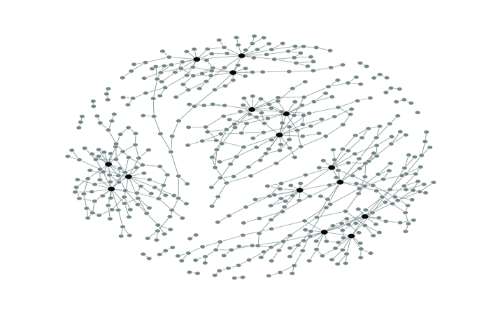
(a) Hub network: 500 nodes and 568 edges. 15 nodes (in black) have degrees of around 15.

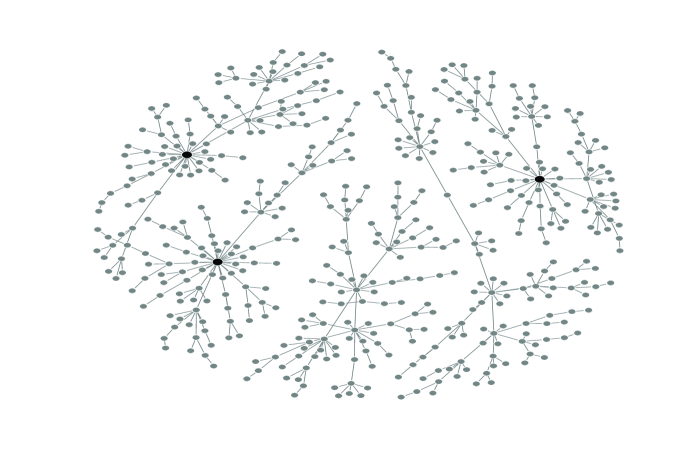
(b) Power-law network: 500 nodes and 495 edges. 3 nodes (in black) have degrees at least 20.

Figure 1: Topology of simulated networks.

Hub networks  In the first set of simulations, module networks are generated by inserting a few hub nodes into a very sparse graph. Specifically, each module consists of three hubs with degrees around $15$, and the other $97$ nodes with degrees at most four. This setting is designed to mimic the genetic regulatory networks, which usually contains a few hub genes plus many other genes with only a few edges. A network consisting of five such modules is shown in Figure 1(a). In this network, there are $p=500$ nodes and $568$ edges. The simulated non-zero partial correlations fall in $(-0.67,-0.1]\cup[0.1,0.67)$, with two modes around -0.28 and 0.28. Based on this network and the partial correlation matrix, we generate $50$ independent data sets each consisting of $n=250$ i.i.d. samples.

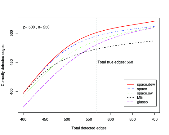
(a) x-axis: the number of total detected edges(i.e., the total number of pairs $(i,j)$ with $\widehat{\rho}^{ij}\not=0$); y-axis: the number of correctly identified edges. The vertical grey line corresponds to the number of true edges.

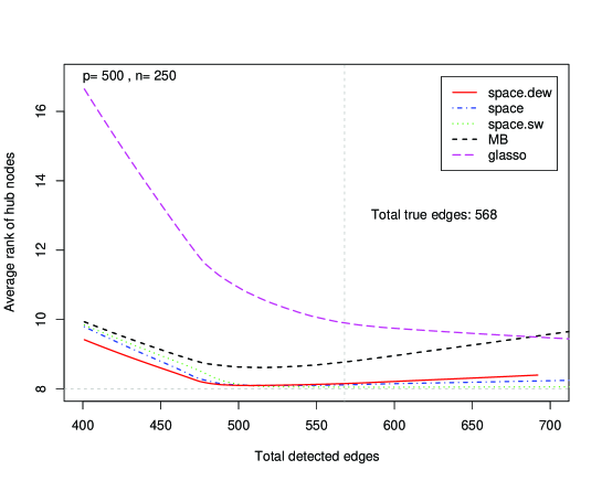
(b) x-axis: the number of total detected edges; y-axis: the average rank of the estimated degrees of the 15 true hub nodes.

Figure 2: Simulation results for Hub network.

We then evaluate each method at a series of different values of the tuning parameter $\lambda$. The number of total detected edges ($N_{t}$) decreases as $\lambda$ increases. Figure 2(a) shows the number of correctly detected edges ($N_{c}$) vs. the number of total detected edges ($N_{t}$) averaged across the $50$ independent data sets for each method. We observe that all three space methods (space, space.sw and space.dew) consistently detect more correct edges than the neighborhood selection method MB (except for space.sw when $N_{t}<470$) and the likelihood based method glasso. MB performs favorably over glasso when $N_{t}$ is relatively small (say less than $530$), but performs worse than glasso when $N_{t}$ is large. Overall, space.dew is the best among all methods. Specifically, when $N_{t}=568$ (which is the number of true edges), space.dew detects $501$ correct edges on average with a standard deviation $4.5$ edges. The corresponding sensitivity and specificity are both $88\%$. Here, sensitivity is defined as the ratio of the number of correctly detected edges to the total number of true edges; and specificity is defined as the ratio of the number of correctly detected edges to the number of total detected edges. On the other hand, MB and glasso detect $472$ and $480$ correct edges on average, respectively, when the number of total detected edges $N_{t}$ is $568$.

In terms of hub detection, for a given $N_{t}$, a rank is assigned to each variable $y_{i}$ based on its estimated degree (the larger the estimated degree, the smaller the rank value). We then calculate the average rank of the $15$ true hub nodes for each method. The results are shown in Figure 2(b). This average rank would achieve the minimum value $8$ (indicated by the grey horizontal line), if the $15$ true hubs have larger estimated degrees than all other non-hub nodes. As can be seen from the figure, the average rank curves (as a function of $N_{t}$) for the three space methods are very close to the optimal minimum value $8$ for a large range of $N_{t}$. This suggests that these methods can successfully identify most of the true hubs. Indeed, for space.dew, when $N_{t}$ equals to the number of true edges ($568$), the top $15$ nodes with the highest estimated degrees contain at least $14$ out of the $15$ true hub nodes in all replicates. On the other hand, both MB and glasso identify far fewer hub nodes, as their corresponding average rank curves are much higher than the grey horizontal line.

Table 2: Power (sensitivity) of space.dew , MB and glasso in identifying correct edges when FDR is controlled at 0.05.

Network	$p$	$n$	space.dew	MB	glasso
Hub-network	500	250	0.844	0.784	0.655
		200	0.707	0.656	0.559
Hub-network	1000	300	0.856	0.790	0.690
		500	0.963	0.894	0.826
Power-law network	500	250	0.704	0.667	0.580

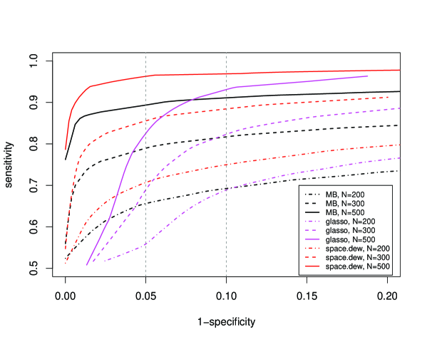
Figure 3: Hub network: ROC curves for different samples sizes ($p=1000$).

To investigate the impact of dimensionality $p$ and sample size $n$, we perform simulation studies for a larger dimension with $p=1000$ and various sample sizes with $n=200,300$ and $500$. The simulated network includes ten disjointed modules of size $100$ each and has $1163$ edges in total. Non-zero partial correlations form a similar distribution as that of the $p=500$ network discussed above. The ROC curves for space.dew, MB and glasso resulted from these simulations are shown in Figure 3. When false discovery rate (=1-specificity) is controlled at $0.05$, the power (=sensitivity) for detecting correct edges is given in Table 2. From the figure and the table, we observe that the sample size has a big impact on the performance of all methods. For $p=1000$, when the sample size increases from $200$ to $300$, the power of space.dew increases more than $20\%$; when the sample size is $500$, space.dew achieves an impressive power of $96\%$. On the other hand, the dimensionality seems to have relatively less influence. When the total number of variables is doubled from $500$ to $1000$, with only $20\%$ more samples (that is $p=500,n=250$ vs. $p=1000,n=300$), all three methods achieve similar powers. This is presumably because the larger network ($p=1000$) is sparser than the smaller network ($p=500$) and also the complexity of the modules remains unchanged. Finally, it is obvious from Figure 3 that, space.dew performs best among the three methods.

Table 3: Edge detection under the selected tuning parameter $\lambda$. For average rank, the optimal value is $15.5$. For MB.alpha, $\alpha=0.05$ is used.

Sample size	Method	Total edge detected	Sensitivity	Specificity	Average rank
	space.joint	1357	0.821	0.703	28.6
$n=200$	MB.sep	1240	0.751	0.703	57.5
	MB.alpha	404	0.347	1.00	175.8
	glasso.like	1542	0.821	0.619	35.4
	space.joint	1481	0.921	0.724	18.2
$n=300$	MB.sep	1456	0.867	0.692	30.4
	MB.alpha	562	0.483	1.00	128.9
	glasso.like	1743	0.920	0.614	21
	space.joint	1525	0.980	0.747	16.0
$n=500$	MB.sep	1555	0.940	0.706	16.9
	MB.alpha	788	0.678	1.00	52.1
	glasso.like	1942	0.978	0.586	16.5

We then investigate the performance of these methods at the selected tuning parameters (see Section 2.4 for details). For the above Hub network with $p=1000$ nodes and $n=200,300,500$, the results are reported in Table 3. As can be seen from the table, BIC based approaches tend to select large models (compared to the true model which has $1163$ edges). space.joint and MB.sep perform similarly in terms of specificity, and glasso.like works considerably worse than the other two in this regard. On the other hand, space.joint and glasso.like performs similarly in terms of sensitivity, and are better than MB.sep on this aspect. In contrast, MB.alpha selects very small models and thus results in very high specificity, but very low sensitivity. In terms of hub identification, space.joint apparently performs better than other methods (indicated by a smaller average rank over $30$ true hub nodes). Moreover, the performances of all methods improve with sample size.

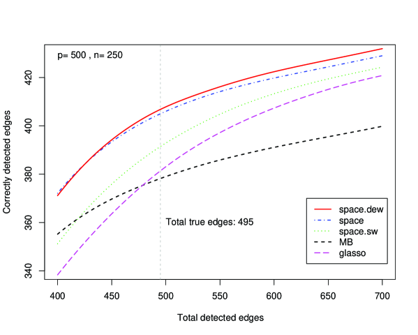
Figure 4: Simulation results for Power-law network. x-axis: the number of total detected edges; y-axis: the number of correctly identified edges. The vertical grey line corresponds to the number of true edges.

Power-law networks   Many real world networks have a power-law (also a.k.a scale-free) degree distribution with an estimated power parameter $\alpha=2\sim 3$ newman. Thus, in the second set of simulations, the module networks are generated according to a power-law degree distribution with the power-law parameter $\alpha=2.3$, as this value is close to the estimated power parameters for biological networks newman. Figure 1(b) illustrates a network formed by five such modules with each having $100$ nodes. It can be seen that there are three obvious hub nodes in this network with degrees of at least $20$. The simulated non-zero partial correlations fall in the range $(-0.51,-0.08]\cup[0.08,0.51)$, with two modes around -0.22 and 0.22. Similar to the simulation done for Hub networks, we generate $50$ independent data sets each consisting of $n=250$ i.i.d. samples. We then compare the number of correctly detected edges by various methods. The result is shown in Figure 4. On average, when the number of total detected edges equals to the number of true edges which is $495$, space.dew detects $406$ correct edges, while MB detects only $378$ and glasso detects only $381$ edges. In terms of hub detection, all methods can correctly identify the three hub nodes for this network.

Summary   These simulation results suggest that when the (concentration) networks are reasonably sparse, we should be able to characterize their structures with only a couple-of-hundreds of samples when there are a couple of thousands of nodes. In addition, space.dew outperforms MB by at least $6\%$ on the power of edge detection under all simulation settings above when FDR is controlled at $0.05$, and the improvements are even larger when FDR is controlled at a higher level say $0.1$ (see Figure 3). Also, compared to glasso, the improvement of space.dew is at least $15\%$ when FDR is controlled at $0.05$, and the advantages become smaller when FDR is controlled at a higher level (see Figure 3). Moreover, the space methods perform much better in hub identification than both MB and glasso.

Simulation Study II

In the second simulation study, we apply space, MB and glasso on networks with nearly uniform degree distributions generated by following the simulation procedures in meinshausen; as well as on the AR network discussed in Yuan and TiSparse07. For these cases, space performs comparably, if not better than, the other two methods. However, for these networks without hubs, the advantages of space become smaller compared to the results on the networks with hubs. The results are summarized below.

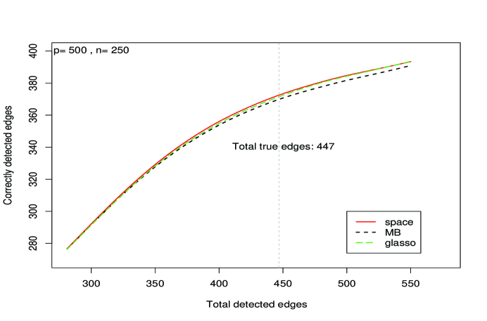
(b) Simulation results for Uniform network. x-axis: the total number of edges detected; y-axis: the total number of correctly identified edges. The vertical grey line corresponds to the number of true edges.

Figure 5: Simulation results for Uniform networks.

Uniform networks   In this set of simulation, we generate similar networks as the ones used in meinshausen. These networks have uniform degree distribution with degrees ranging from zero to four. Figure 5(a) illustrates a network formed by five such modules with each having $100$ nodes. There are in total $447$ edges. Figure 5(b) illustrates the performance of $\texttt{MB},\texttt{space}$ and glasso over $50$ independent data sets each having $n=250$ i.i.d. samples. As can be been from this figure, all three methods perform similarly. When the total number of detected edges equals to the total number of true edges ($447$), space detects $372$ true edges, MB detects $369$ true edges and glasso $371$ true edges.

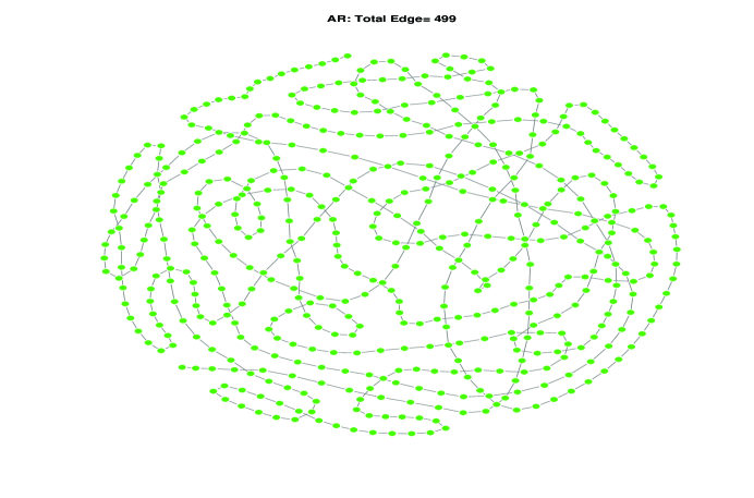
(a) AR network: 500 nodes and 499 edges.

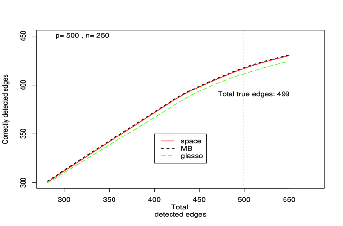
(b) Simulation results for AR network. x-axis: the total number of edges detected; y-axis: the total number of correctly identified edges. The vertical grey line corresponds to the number of true edges.

Figure 6: Simulation results for AR networks.

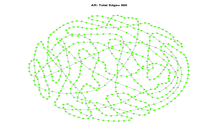
(a) Big-circle network: 500 nodes and 500 edges.

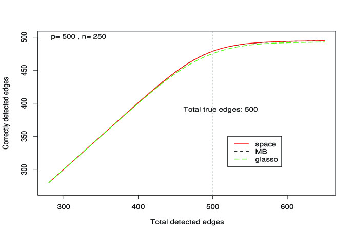
(b) Simulation results for Circle network. x-axis: the total number of edges detected; y-axis: the total number of correctly identified edges. The vertical grey line corresponds to the number of true edges.

Figure 7: Simulation results for Circle networks.

AR networks   In this simulation, we consider the so called AR network used in Yuan and TiSparse07. Specifically, we have $\sigma^{ii}=1$ for $i=1,\cdots p$ and $\sigma^{i-1,i}=\sigma^{i,i-1}=0.25$ for $i=2,\cdots,p$. Figure 6(a) illustrates such a network with $p=500$ nodes and thus $499$ edges. Figure 6(b) illustrates the performance of $\texttt{MB},\texttt{space}$ and glasso over $50$ independent data sets each having $n=250$ i.i.d. samples. As can be been from this figure, all three methods again perform similarly. When the total number of detected edges equals to the total number of true edges ($499$), space detects $416$ true edges, MB detects $417$ true edges and glasso $411$ true edges. As a slight modification of the AR network, we also consider a big circle network with: $\sigma^{ii}=1$ for $i=1,\cdots p$; $\sigma^{i-1,i}=\sigma^{i,i-1}=0.3$ for $i=2,\cdots,p$ and $\sigma^{1,p}=\sigma^{p,1}=0.3$. Figure 7(a) illustrates such a network with $p=500$ nodes and thus $500$ edges. Figure 7(b) compares the performance of the three methods. When the total number of detected edges equals to the total number of true edges ($500$), space, MB and glasso detect $478$, $478$ and $475$ true edges, respectively.

We also compare the mean squared error (MSE) of estimation of $\{\sigma^{ii}\}$. For the uniform network, the median (across all samples and $\lambda$) of the square-root MSE is $0.108,0.113,0.178$ for MB, space and glasso. These numbers are $0.085,0.089,0.142$ for the AR network and $0.128,0.138,0.233$ for the circle network. It seems that MB and space work considerably better than glasso on this aspect.

Comments

We conjecture that, under the sparse and high dimensional setting, the superior performance in model selection of the regression based method space over the penalized likelihood method glasso is partly due to its simpler quadratic loss function. Moreover, since space ignores the correlation structure of the regression residuals, it amounts to a greater degree of regularization, which may render additional benefits under the sparse and high dimensional setting.

In terms of parameter estimation, we compare the entropy loss of the three methods. We find that, they perform similarly when the estimated models are of small or moderate size. When the estimated models are large, glasso generally performs better in this regard than the other two methods. Since the interest of this paper lies in model selection, detailed results of parameter estimation are not reported here.

As discussed earlier, one limitation of space is its lack of assurance of positive definiteness. However, for simulations reported above, the corresponding estimators we have examined (over $3000$ in total) are all positive definite. To further investigate this issue, we design a few additional simulations. We first consider a case with a similar network structure as the Hub network, however having a nearly singular concentration matrix (the condition number is $16,240$; as a comparison, the condition number for the original Hub network is $62$). For this case, the estimate of space remains positive definite until the number of total detected edges increases to $50,000$; while the estimate of MB remains positive definite until the number of total detected edges is more than $23,000$. Note that, the total number of true edges of this model is only $568$, and the model selected by space.joint has $791$ edges. In the second simulation, we consider a denser network ($p=500$ and the number of true edges is $6,188$) with a nearly singular concentration matrix (condition number is $3,669$). Again, we observe that, the space estimate only becomes non-positive-definite when the estimated models are huge (the number of detected edges is more than $45,000$). This suggests that, for the regime we are interested in in this paper (the sparse and high dimensional setting), non-positive-definiteness does not seem to be a big issue for the proposed method, as it only occurs when the resulting model is huge and thus very far away from the true model. As long as the estimated models are reasonably sparse, the corresponding estimators by space remain positive definite. We believe that this is partly due to the heavy shrinkage imposed on the off-diagonal entries in order to ensure sparsity.

Finally, we investigate the performance of these methods when the observations come from a non-normal distribution. Particularly, we consider the multivariate $t_{df}$-distribution with $df=3,6,10$. The performances of all three methods deteriorate compared to the normal case, however the overall picture in terms of relative performance among these methods remains essentially unchanged (Table 4).

Table 4: Sensitivity of different methods under different $t_{df}$-distributions when FDR is controlled at 0.05

		Sensitivity
df	Method	Hub	Power-law
	space	0.369	0.286
3	MB	0.388	0.276
	glasso	0.334	0.188
	space	0.551	0.392
6	MB	0.535	0.390
	glasso	0.471	0.293
	space	0.682	0.512
10	MB	0.639	0.518
	glasso	0.598	0.345

4 APPLICATION

More than 500,000 women die annually of breast cancer world wide. Great efforts are being made to improve the prevention, diagnosis and treatment for breast cancer. Specifically, in the past couple of years, molecular diagnostics of breast cancer have been revolutionized by high throughput genomics technologies. A large number of gene expression signatures have been identified (or even validated) to have potential clinical usage. However, since breast cancer is a complex disease, the tumor process cannot be understood by only analyzing individual genes. There is a pressing need to study the interactions between genes, which may well lead to better understanding of the disease pathologies.

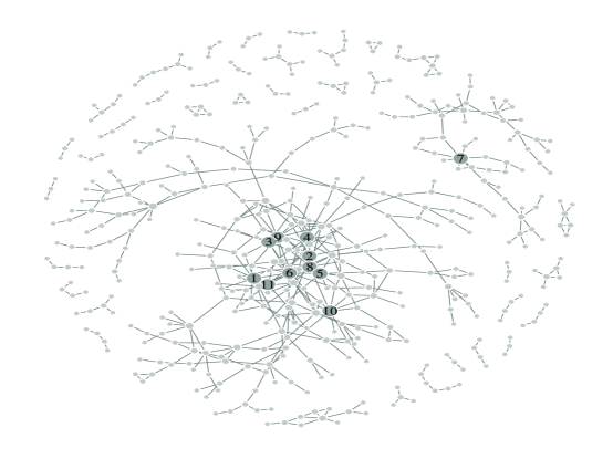
(a) Network inferred from the real data (only showing components with at least three nodes). The gene annotation of the hub nodes (numbered) are given in Table 5.

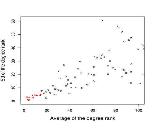
(b) Degree ranks (for the 100 genes with highest degrees). Different circles represent different genes. Solid circles: the 11 genes with highest degrees. Circles: the other genes. The sd(rank) of the top 11 genes are all smaller than $4.62$ ($4.62$ is the $1\%$ quantile of sd(rank) among all the 1217 genes), and thus are identified as hub nodes.

Figure 8: Results for the breast cancer expression data set.

In a recent breast cancer study, microarray expression experiments were conducted for $295$ primary invasive breast carcinoma samples Chang2005,VanDe2002. Raw array data and patient clinical outcomes for $244$ of these samples are available on-line and are used in this paper. Data can be downloaded at http://microarray-pubs.stanford.edu/wound_NKI/explore.html . To globally characterize the association among thousands of mRNA expression levels in this group of patients, we apply the space method on this data set as follows. First, for each expression array, we perform the global normalization by centering the mean to zero and scaling the median absolute deviation to one. Then we focus on a subset of $p=1217$ genes/clones whose expression levels are significantly associated with tumor progression ($p$-values from univariate Cox models $<$ 0.0008, corresponding FDR $=0.01$). We estimate the partial correlation matrix of these $1217$ genes with space.dew for a series of $\lambda$ values. The degree distribution of the inferred network is heavily skewed to the right. Specifically, when $629$ edges are detected, $598$ out of the $1217$ genes do not connect to any other genes, while five genes have degrees of at least 10. The power-law parameter of this degree distribution is $\alpha=2.56$ , which is consistent with the findings in the literature for GRNs  newman. The topology of the inferred network is shown in Figure 8(a), which supports the statement that genetic pathways consist of many genes with few interactions and a few hub genes with many interactions.

We then search for potential hub genes by ranking nodes according to their degrees. There are 11 candidate hub genes whose degrees consistently rank the highest under various $\lambda$ [see Figure 8(b)]. Among these 11 genes, five are important known regulators in breast cancer. For example, HNF3A (also known as FOXA1) is a transcription factor expressed predominantly in a subtype of breast cancer, which regulates the expression of the cell cycle inhibitor $p27kip1$ and the cell adhesion molecule E-cadherin. This gene is essential for the expression of approximately $50\%$ of estrogene-regulated genes and has the potential to serve as a therapeutic target Nakshatri2007. Except for HNF3A, all the other 10 hub genes fall in the same big network component related to cell cycle/proliferation. This is not surprising as it is well-agreed that cell cycle/proliferation signature is prognostic for breast cancer. Specifically, KNSL6, STK12, RAD54L and BUB1 have been previously reported to play a role in breast cancer: KNSL6 (also known as KIF2C) is important for anaphase chromosome segregation and centromere separation, which is overexpressed in breast cancer cells but expressed undetectably in other human tissues except testis Shimo2007; STK12 (also known as AURKB) regulates chromosomal segregation during mitosis as well as meiosis, whose LOH contributes to an increased breast cancer risk and may influence the therapy outcome Tchatchou2007; RAD54L is a recombinational repair protein associated with tumor suppressors BRCA1 and BRCA2, whose mutation leads to defect in repair processes involving homologous recombination and triggers the tumor development Matsuda1999; in the end, BUB1 is a spindle checkpoint gene and belongs to the BML-1 oncogene-driven pathway, whose activation contributes to the survival life cycle of cancer stem cells and promotes tumor progression. The roles of the other six hub genes in breast cancer are worth of further investigation. The functions of all hub genes are briefly summarized in Table 5.

Table 5: Annotation of hub genes

Index	Gene Symbol	Summary Function (GO)
1	CENPA	Encodes a centromere protein (nucleosome assembly)
2	NA.	Annotation not available
3	KNSL6	Anaphase chromosome segregation (cell proliferation)
4	STK12	Regulation of chromosomal segregation (cell cycle)
5	NA.	Annotation not available
6	URLC9	Annotation not available (up-regulated in lung cancer)
7	HNF3A	Transcriptional factor activity (epithelial cell differentiation)
8	TPX2	Spindle formation (cell proliferation)
9	RAD54L	Homologous recombination related DNA repair (meiosis)
10	ID-GAP	Stimulate GTP hydrolysis (cell cycle)
11	BUB1	Spindle checkpoint (cell cycle)

5 ASYMPTOTICS

In this section, we show that under appropriate conditions, the space procedure achieves both model selection consistency and estimation consistency. Use $\overline{\theta}$ and $\overline{\sigma}$ to denote the true parameters of $\theta$ and $\sigma$. As discussed in Section 2.1, when $\sigma$ is given, $\theta$ is estimated by solving the following $\ell_{1}$ penalization problem:

$$\widehat{\theta}^{\lambda_{n}}(\sigma)={\rm arg}\min_{\theta}L_{n}(\theta,\sigma,\mathbf{Y})+\lambda_{n}||\theta||_{1},$$ (12)

where the loss function $L_{n}(\theta,\sigma,\mathbf{Y}):=\frac{1}{n}\sum_{k=1}^{n}L(\theta,\sigma,\mathbf{Y}^{k}),$ with, for $k=1,\cdots,n$

$$L(\theta,\sigma,\mathbf{Y}^{k}):=\frac{1}{2}\sum_{i=1}^{p}w_{i}(y_{i}^{k}-\sum_{j\not=i}\sqrt{\sigma^{jj}/\sigma{ii}}\rho^{ij}y_{j}^{k})^{2}.$$ (13)

Throughout this section, we assume $\mathbf{Y}^{1},\cdots,\mathbf{Y}^{n}$ are i.i.d. samples from $N_{p}(0,\mathbf{\Sigma})$. The Gaussianity assumption here can be relaxed by assuming appropriate tail behaviors of the observations. The assumption of zero mean is simply for exposition simplicity. In practice, in the loss function (12), $\mathbf{Y}^{k}$ can be replaced by $\mathbf{Y}^{k}-\overline{\mathbf{Y}}$ where $\overline{\mathbf{Y}}=\frac{1}{n}\sum_{k=1}^{n}\mathbf{Y}^{k}$ is the sample mean. All results stated in this section still hold under that case.

We first state regularity conditions that are needed for the proof. Define $\mathcal{A}=\{(i,j):\overline{\rho}^{ij}\not=0\}$.

• The weights satisfy $0<w_{0}\leq\min_{i}\{w_{i}\}\leq\max_{i}\{w_{i}\}\leq w_{\infty}<\infty$

• There exist constants $0<\Lambda_{\min}(\overline{\theta})\leq\Lambda_{\max}(\overline{\theta})<\infty$, such that the true covariance $\overline{\mathbf{\Sigma}}=\overline{\mathbf{\Sigma}}(\overline{\theta},\overline{\sigma})$ satisfies: $0<\Lambda_{\min}(\overline{\theta})\leq\lambda_{\min}(\overline{\mathbf{\Sigma}})\leq\lambda_{\max}(\overline{\mathbf{\Sigma}})\leq\Lambda_{\max}(\overline{\theta})<\infty,$ where $\lambda_{\min}$ and $\lambda_{\max}$ denote the smallest and largest eigenvalues of a matrix, respectively.

• There exist a constant $\delta<1$ such that for all $(i,j)\notin\mathcal{A}$

  $$\left|\overline{L}^{\prime\prime}_{ij,\mathcal{A}}(\overline{\theta},\overline{\sigma})\left[\overline{L}^{\prime\prime}_{\mathcal{A},\mathcal{A}}(\overline{\theta},\overline{\sigma})\right]^{-1}{\rm sign}(\overline{\theta}_{\mathcal{A}})\right|\leq\delta(<1),$$

  where for $1\leq i<j\leq p,1\leq t<s\leq p$,

  $$\overline{L}^{\prime\prime}_{ij,ts}(\overline{\theta},\overline{\sigma}):=E_{(\overline{\theta},\overline{\sigma})}\left(\frac{\partial^{2}L(\theta,\sigma,Y)}{\partial\rho^{ij}\partial\rho^{ts}}\Bigl{|}_{\theta=\overline{\theta},\sigma=\overline{\sigma}}\right).$$

Condition C0 says that the weights are bounded away from zero and infinity. Condition C1 assumes that the eigenvalues of the true covariance matrix $\overline{\mathbf{\Sigma}}$ are bounded away from zero and infinity. Condition C2 corresponds to the incoherence condition in meinshausen, which plays a crucial role in proving model selection consistency of $\ell_{1}$ penalization problems.

Furthermore, since $\overline{\sigma}$ is usually unknown, it needs to be estimated. Use $\widehat{\sigma}=\widehat{\sigma}_{n}=\{\widehat{\sigma}^{ii}\}_{i=1}^{p}$ to denote one estimator. The following condition says

• : For any $\eta>0$, there exists a constant $C>0$, such that for sufficiently large $n$, $\max_{1\leq i\leq p}|\widehat{\sigma}^{ii}-\overline{\sigma}^{ii}|\leq C(\sqrt{\frac{\log n}{n}})$ holds with probability at least $1-O(n^{-\eta})$.

Note that, the theorems below hold even when $\widehat{\sigma}$ is obtained based on the same data set from which $\theta$ is estimated as long as condition D is satisfied. The following proposition says that, when $p<n$, we can get an estimator of $\sigma$ satisfying condition D by simply using the residuals of the ordinary least square fitting.

Proposition 1

Suppose $\mathbf{Y}=[\mathbf{Y}^{1}:\cdots:\mathbf{Y}^{n}]$ is a $p\times n$ data matrix with i.i.d. columns $\mathbf{Y}^{i}\sim N_{p}(0,\mathbf{\Sigma})$. Further suppose that $p=p_{n}$ such that $p/n\leq 1-\delta$ for some $\delta>0$; and $\mathbf{\Sigma}$ has a bounded condition number (that is assuming condition C1). Let $\overline{\sigma}^{ii}$ denote the $(i,i)$-th element of $\mathbf{\Sigma}^{-1}$; and let $\mathbf{e}_{i}$ denote the residual from regressing $\mathbf{Y}^{i}$ on to $\mathbf{Y}_{(-i)}:=[\mathbf{Y}^{1}:\cdots:\mathbf{Y}^{i-1}:\mathbf{Y}^{i+1}:\cdots:\mathbf{Y}^{n}]$, that is

$$\mathbf{e}_{i}=\mathbf{Y}^{i}-\mathbf{Y}_{(-i)}^{T}(\mathbf{Y}_{(-i)}\mathbf{Y}_{(-i)}^{T})^{-1}\mathbf{Y}_{(-i)}\mathbf{Y}^{i}.$$

Define $\widehat{\sigma}^{ii}=1/\widehat{\sigma}_{ii,-(i)}$, where

$$\widehat{\sigma}_{ii,-(i)}=\frac{1}{n-p-1}\mathbf{e}_{i}^{T}\mathbf{e}_{i},$$

then condition D holds for $\{\widehat{\sigma}^{ii}\}_{i=1}^{p}$.

The proof of this proposition is omitted due to space limitation.

We now state notations used in the main results. Let $q_{n}=|\mathcal{A}|$ denote the number of nonzero partial correlations (of the underlying true model) and let $\{s_{n}\}$ be a positive sequence of real numbers such that for any $(i,j)\in\mathcal{A}$: $|\overline{\rho}^{ij}|\geq s_{n}.$ Note that, $s_{n}$ can be viewed as the signal size. We follow the similar strategy as in meinshausen and Massam2007 in deriving the asymptotic result: (i) First prove estimation consistency and sign consistency for the restricted penalization problem with $\theta_{\mathcal{A}^{c}}=0$ (Theorem 1). We employ the method of the proof of Theorem 1 in Fan2004; (ii) Then we prove that with probability tending to one, no wrong edge is selected (Theorem 2); (iii) The final consistency result then follows (Theorem 3).

Theorem 1

(consistency of the restricted problem) Suppose that conditions C0-C1 and D are satisfied. Suppose further that $q_{n}\sim o(\sqrt{\frac{n}{\log n}}),\ \lambda_{n}\sqrt{\frac{n}{\log n}}\rightarrow\infty$ and $\sqrt{q_{n}}\lambda_{n}\sim o(1)$, as $n\rightarrow\infty$. Then there exists a constant $C(\overline{\theta})>0$, such that for any $\eta>0$, the following events hold with probability at least $1-O(n^{-\eta})$:

• there exists a solution $\widehat{\theta}^{\mathcal{A},\lambda_{n}}=\widehat{\theta}^{\mathcal{A},\lambda_{n}}(\widehat{\sigma})$ of the restricted problem:

  $$\min_{\theta:\theta_{\mathcal{A}^{c}}=0}L_{n}(\theta,\widehat{\sigma},\mathbf{Y})+\lambda_{n}||\theta||_{1},$$ (14)

  where the loss function $L_{n}$ is defined via (13).

• (estimation consistency) any solution $\widehat{\theta}^{\mathcal{A},\lambda_{n}}$ of the restricted problem (14) satisfies:

  $$||\widehat{\theta}^{\mathcal{A},\lambda_{n}}-\overline{\theta}_{\mathcal{A}}||_{2}\leq C(\overline{\theta})\sqrt{q_{n}}\lambda_{n}.$$

• (sign consistency) if further assume that the signal sequence satisfies: $\frac{s_{n}}{\sqrt{q_{n}}\lambda_{n}}\rightarrow\infty,\ n\rightarrow\infty$, then ${\rm sign}(\widehat{\theta}^{\mathcal{A},\lambda_{n}}_{ij})={\rm sign}(\overline{\theta}_{ij})$, for all $1\leq i<j\leq p$.

Theorem 2

Suppose that conditions C0-C2 and D are satisfied. Suppose further that $p=O(n^{\kappa})$ for some $\kappa\geq 0$; $q_{n}\sim o(\sqrt{\frac{n}{\log n}}),\ \sqrt{\frac{q_{n}\log n}{n}}=o(\lambda_{n}),\ \lambda_{n}\sqrt{\frac{n}{\log n}}\rightarrow\infty$ and $\sqrt{q_{n}}\lambda_{n}\sim o(1)$, as $n\rightarrow\infty$. Then for any $\eta>0$, for $n$ sufficiently large, the solution of (14) satisfies

$$P_{(\overline{\theta},\overline{\sigma})}\left(\max_{(i,j)\in\mathcal{A}^{c}}|L^{\prime}_{n,ij}(\widehat{\theta}^{\mathcal{A},\lambda_{n}},\widehat{\sigma},\mathbf{Y})|<\lambda_{n}\right)\geq 1-O(n^{-\eta}),$$

where $L^{\prime}_{n,ij}:=\frac{\partial L_{n}}{\partial\rho^{ij}}.$

Theorem 3

Assume the same conditions of Theorem 2. Then there exists a constant $C(\overline{\theta})>0$, such that for any $\eta>0$ the following events hold with probability at least $1-O(n^{-\eta})$:

• there exists a solution $\widehat{\theta}^{\lambda_{n}}=\widehat{\theta}^{\lambda_{n}}(\widehat{\sigma})$ of the $\ell_{1}$ penalization problem

  $$\min_{\theta}L_{n}(\theta,\widehat{\sigma},\mathbf{Y})+\lambda_{n}||\theta||_{1},$$ (15)

  where the loss function $L_{n}$ is defined via (13).

• (estimation consistency): any solution $\widehat{\theta}^{\lambda_{n}}$ of (15) satisfies:

  $$||\widehat{\theta}^{\lambda_{n}}-\overline{\theta}||_{2}\leq C(\overline{\theta})(\sqrt{q_{n}}\lambda_{n}).$$

• (Model selection consistency/sign consistency):

  $${\rm sign}(\widehat{\theta}^{\lambda_{n}}_{ij})={\rm sign}(\overline{\theta}_{ij}),\ \hbox{for all $1\leq i<j\leq p$}.$$

Proofs of these theorems are given in the Supplemental Material. Finally, due to exponential small tails of the probabilistic bounds, model selection consistency can be easily extended when the network consists of $N$ disjointed components with $N=O(n^{\alpha})$ for some $\alpha\geq 0$, as long as the size and the number of true edges of each component satisfy the corresponding conditions in Theorem 2.

Remark 2

The condition $\lambda_{n}\sqrt{\frac{n}{\log n}}\rightarrow\infty$ is indeed implied by the condition $\sqrt{\frac{q_{n}\log n}{n}}=o(\lambda_{n})$ as long as $q_{n}$ does not go to zero. Moreover, under the “worst case” scenario, that is when $q_{n}$ is almost in the order of $\sqrt{\frac{n}{\log n}}$, $\lambda_{n}$ needs to be nearly in the order of $n^{-1/4}$. On the other hand, for the“best case” scenario, that is when $q_{n}=O(1)$ (for example, when the dimension $p$ is fixed), the order of $\lambda_{n}$ can be nearly as small as $n^{-1/2}$ (within a factor of $\log n$). Consequently, the $\ell_{2}$-norm distance of the estimator from the true parameter is in the order of $\sqrt{\log n/n}$, with probability tending to one.

6 SUMMARY

In this paper, we propose a joint sparse regression model – space – for selecting non-zero partial correlations under the high-dimension-low-sample-size setting. By controlling the overall sparsity of the partial correlation matrix, space is able to automatically adjust for different neighborhood sizes and thus to utilize data more effectively. The proposed method also explicitly employs the symmetry among the partial correlations, which also helps to improve efficiency. Moreover, this joint model makes it easy to incorporate prior knowledge about network structure. We develop a fast algorithm active-shooting to implement the proposed procedure, which can be readily extended to solve some other penalized optimization problems. We also propose a “BIC-type” criterion for the selection of the tuning parameter. With extensive simulation studies, we demonstrate that this method achieves good power in non-zero partial correlation selection as well as hub identification, and also performs favorably compared to two existing methods. The impact of the sample size and dimensionality has been examined on simulation examples as well. We then apply this method on a microarray data set of $1217$ genes from $244$ breast cancer tumor samples, and find $11$ candidate hubs, of which five are known breast cancer related regulators. In the end, we show consistency (in terms of model selection and estimation) of the proposed procedure under suitable regularity and sparsity conditions.

The R package space – Sparse PArtial Correlation Estimation – is available on cran.

(a) Uniform network: 500 nodes and 447 edges.

Supplemental Material

Part I

In this section, we list properties of the loss function:

$$L(\theta,\sigma,Y)=\frac{1}{2}\sum_{i=1}^{p}w_{i}(y_{i}-\sum_{j\not=i}\sqrt{\sigma^{jj}/\sigma{ii}}\rho^{ij}y_{j})^{2}=\frac{1}{2}\sum_{i=1}^{p}\tilde{w}_{i}(\tilde{y}_{i}-\sum_{j\not=i}\rho^{ij}\tilde{y}_{j})^{2},$$ (S-1)

where $Y=(y_{1},\cdots,y_{p})^{T}$ and $\tilde{y}_{i}=\sqrt{\sigma^{ii}}y_{i}$,$\tilde{w}_{i}=w_{i}/\sigma^{ii}$. These properties are used for the proof of the main results. Note: throughout the supplementary material, when evaluation is taken place at $\sigma=\bar{\sigma}$, sometimes we omit the argument $\sigma$ in the notation for simplicity. Also we use $Y=(y_{1},\cdots,y_{p})^{T}$ to denote a generic sample and use $\mathbf{Y}$ to denote the $p\times n$ data matrix consisting of $n$ i.i.d. such samples: $\mathbf{Y^{1}},\cdots,\mathbf{Y^{n}}$, and define

$$L_{n}(\theta,\sigma,\mathbf{Y}):=\frac{1}{n}\sum_{k=1}^{n}L(\theta,\sigma,\mathbf{Y}^{k}).$$ (S-2)

• for all $\theta,\sigma$ and $Y\in\mathcal{R}^{p}$, $L(\theta,\sigma,Y)\geq 0.$

• for any $Y\in\mathcal{R}^{p}$ and any $\sigma>0$, $L(\cdot,\sigma,Y)$ is convex in $\theta$; and with probability one, $L(\cdot,\sigma,Y)$ is strictly convex.

• for $1\leq i<j\leq p$

  $$\overline{L}^{\prime}_{ij}(\bar{\theta},\bar{\sigma}):=E_{(\bar{\theta},\bar{\sigma})}\left(\frac{\partial L(\theta,\sigma,Y)}{\partial\rho^{ij}}\Bigl{|}_{\theta=\bar{\theta},\sigma=\bar{\sigma}}\right)=0.$$

• for $1\leq i<j\leq p$ and $1\leq k<l\leq p$,

  $$\overline{L}_{ij,kl}^{{}^{\prime\prime}}(\theta,\sigma):=E_{(\theta,\sigma)}\left(\frac{\partial^{2}L(\theta,\sigma,Y)}{\partial\rho^{ij}\rho^{kl}}\right)=\frac{\partial}{\partial\rho^{kl}}\left[E_{(\theta,\sigma)}\left(\frac{\partial L(\theta,\sigma,Y)}{\partial\rho^{ij}}\right)\right],$$

  and $\overline{L}^{{}^{\prime\prime}}(\bar{\theta},\bar{\sigma})$ is positive semi-definite.

If assuming C0-C1, then we have

• : There exist constants $0<\bar{\sigma}_{0}\leq\bar{\sigma}_{\infty}<\infty$ such that: $0<\bar{\sigma}_{0}\leq\min\{\bar{\sigma}^{ii}:1\leq i\leq p\}\leq\max\{\bar{\sigma}^{ii}:1\leq i\leq p\}\leq\bar{\sigma}_{\infty}$.

• : There exist constants $0<\Lambda^{L}_{\min}(\bar{\theta})\leq\Lambda^{L}_{\max}(\bar{\theta})<\infty$, such that

  $$0<\Lambda^{L}_{\min}(\bar{\theta})\leq\lambda_{min}(\overline{L}^{\prime\prime}(\bar{\theta}))\leq\lambda_{\max}(\overline{L}^{\prime\prime}(\bar{\theta}))\leq\Lambda^{L}_{\max}(\bar{\theta})<\infty$$

• : There exists a constant $K(\bar{\theta})<\infty$, such that for all $1\leq i<j\leq p$, $\overline{L}_{ij,ij}^{\prime\prime}(\bar{\theta})\leq K(\bar{\theta}).$

• : There exist constants $M_{1}(\bar{\theta}),M_{2}(\bar{\theta})<\infty$, such that for any $1\leq i<j\leq p$

  $${\rm Var}_{(\bar{\theta},\bar{\sigma})}(L^{\prime}_{ij}(\bar{\theta},\bar{\sigma},Y))\leq M_{1}(\bar{\theta}),\ {\rm Var}_{(\bar{\theta},\bar{\sigma})}(L^{\prime\prime}_{ij,ij}(\bar{\theta},\bar{\sigma},Y))\leq M_{2}(\bar{\theta}).$$

• : There exists a constant $0<g(\bar{\theta})<\infty$, such that for all $(i,j)\in\mathcal{A}$

  $$\overline{L}^{\prime\prime}_{ij,ij}(\bar{\theta},\bar{\sigma})-\overline{L}^{\prime\prime}_{ij,\mathcal{A}_{ij}}(\bar{\theta},\bar{\sigma})\left[\overline{L}^{\prime\prime}_{\mathcal{A}_{ij},\mathcal{A}_{ij}}(\bar{\theta},\bar{\sigma})\right]^{-1}\overline{L}^{\prime\prime}_{\mathcal{A}_{ij},ij}(\bar{\theta},\bar{\sigma})\geq g(\bar{\theta}),$$

  where $\mathcal{A}_{ij}=\mathcal{A}/\{(i,j)\}$.

• : There exists a constant $M(\bar{\theta})<\infty$, such that for any $(i,j)\in\mathcal{A}^{c}$

  $$||\overline{L}^{\prime\prime}_{ij,\mathcal{A}}(\bar{\theta})[\overline{L}^{\prime\prime}_{\mathcal{A}\mathcal{A}}(\bar{\theta})]^{-1}||_{2}\leq M(\bar{\theta}).$$

• There exists a constant $K_{1}(\bar{\theta})<\infty$, such that for any $1\leq i\leq j\leq p$, $||E_{\bar{\theta}}(\tilde{y}_{i}\tilde{y}_{j}\tilde{y}\tilde{y}^{T})||\leq K_{1}(\bar{\theta})$, where $\tilde{y}=(\tilde{y}_{1},\cdots,\tilde{y}_{p})^{T}$.

• If we further assume that condition $D$ holds for $\widehat{\sigma}$ and $q_{n}\sim o(\frac{n}{\log n})$, we have: for any $\eta>0$, there exist constants $C_{1,\eta},C_{2,\eta}>0$, such that for sufficiently large $n$

  $$\max_{1\leq i<k\leq p}\left|L^{\prime}_{n,ik}(\bar{\theta},\bar{\sigma},\mathbf{Y})-L^{\prime}_{n,ik}(\bar{\theta},\widehat{\sigma},\mathbf{Y})\right|\leq C_{1,\eta}(\sqrt{\frac{\log n}{n}}),$$

  $$\max_{1\leq i<k\leq p,1\leq t<s\leq p}\left|L^{\prime\prime}_{n,ik,ts}(\bar{\theta},\bar{\sigma},\mathbf{Y})-L^{\prime\prime}_{n,ik,ts}(\bar{\theta},\widehat{\sigma},\mathbf{Y})\right|\leq C_{2,\eta}(\sqrt{\frac{\log n}{n}}),$$

  hold with probability at least $1-O(n^{-\eta})$.

B0 follows from C1 immediately. B1.1–B1.4 are direct consequences of B1. B2 follows from B1 and Gaussianity. B3 follows from conditions C0-C1 and D.

proof of A1: obvious.
proof of A2: obvious.
proof of A3: denote the residual for the ith term by

$$e_{i}(\theta,\sigma)=\tilde{y}_{i}-\sum_{j\not=i}\rho^{ij}\tilde{y}_{j}.$$

Then evaluated at the true parameter values $(\bar{\theta},\bar{\sigma})$, we have $e_{i}(\bar{\theta},\bar{\sigma})$ uncorrelated with $\tilde{y}_{(-i)}$ and $E_{(\bar{\theta},\bar{\sigma})}(e_{i}(\bar{\theta},\bar{\sigma}))=0$. It is easy to show

$$\frac{\partial L(\theta,\sigma,Y)}{\partial\rho^{ij}}=-\tilde{w}_{i}e_{i}(\theta,\sigma)\tilde{y}_{j}-\tilde{w}_{j}e_{j}(\theta,\sigma)\tilde{y}_{i}.$$

This proves A3.
proof of A4: see the proof of B1.

proof of B1: Denote $\tilde{y}=(\tilde{y}_{1},\cdots,\tilde{y}_{p})^{T},$ and $\tilde{x}=(\tilde{x}_{(1,2)},\tilde{x}_{(1,3)},\cdots,\tilde{x}_{(p-1,p)})$ with $\tilde{x}_{(i,j)}=(0,\cdots,0,\tilde{y}_{j},\cdots,\tilde{y}_{i},0,\cdots,0)^{T}.$ Then the loss function (S-1) can be written as $L(\theta,\sigma,Y)=\frac{1}{2}||\tilde{w}(\tilde{y}-\tilde{x}\theta)||^{2}_{2},$ with $\tilde{w}=diag(\sqrt{\tilde{w}}_{1},\cdots,\sqrt{\tilde{w}}_{p})$. Thus $\overline{L}^{\prime\prime}(\theta,\sigma)=E_{(\theta,\sigma)}\left[\tilde{x}^{T}\tilde{w}^{2}\tilde{x}\right]$ (this proves A4). Let $d=p(p-1)/2$, then $\tilde{x}$ is a $p$ by $d$ matrix. Denote its $i$th row by $x_{i}^{T}$ ($1\leq i\leq p$). Then for any $a\in\mathcal{R}^{d}$, with $||a||_{2}=1$, we have

$$a^{T}\overline{L}^{\prime\prime}(\bar{\theta})a=E_{\bar{\theta}}(a^{T}\tilde{x}^{T}\tilde{w}^{2}\tilde{x}a)=E_{\bar{\theta}}\left(\sum_{i=1}^{p}\tilde{w}_{i}(x_{i}^{T}a)^{2}\right).$$

Index the elements of $a$ by $a=(a_{(1,2)},a_{(1,3)},\cdots,a_{(p-1,p)})^{T},$ and for each $1\leq i\leq p$, define $a_{i}\in\mathcal{R}^{p}$ by $a_{i}=(a_{(1,i)},\cdots,a_{(i-1,i)},0,a_{(i,i+1)},\cdots,a_{(i,p)})^{T}.$ Then by definition $x_{i}^{T}a=\tilde{y}^{T}a_{i}.$ Also note that $\sum_{i=1}^{p}||a_{i}||^{2}_{2}=2||a||^{2}_{2}=2.$ This is because, for $i\not=j$, the $jth$ entry of $a_{i}$ appears exactly twice in $a$. Therefore

$$a^{T}\overline{L}^{\prime\prime}(\bar{\theta})a=\sum_{i=1}^{p}\tilde{w}_{i}E_{\bar{\theta}}\left(a_{i}^{T}\tilde{y}\tilde{y}^{T}a_{i}\right)=\sum_{i=1}^{p}\tilde{w}_{i}a_{i}^{T}\tilde{\mathbf{\Sigma}}a_{i}\geq\sum_{i=1}^{p}\tilde{w}_{i}\lambda_{\min}(\tilde{\mathbf{\Sigma}})||a_{i}||^{2}_{2}\geq 2\tilde{w}_{0}\lambda_{\min}(\tilde{\mathbf{\Sigma}}),$$

where $\tilde{\mathbf{\Sigma}}={\rm Var}(\tilde{y})$ and $\tilde{w}_{0}=w_{0}/\bar{\sigma}_{\infty}$. Similarly $a^{T}\overline{L}^{\prime\prime}(\bar{\theta})a\leq 2\tilde{w}_{\infty}\lambda_{\max}(\tilde{\mathbf{\Sigma}}),$ with $\tilde{w}_{\infty}=w_{\infty}/\bar{\sigma}_{0}$. By C1, $\tilde{\mathbf{\Sigma}}$ has bounded eigenvalues, thus B1 is proved.

proof of B1.1: obvious.

proof of B1.2: note that ${\rm Var}_{(\bar{\theta},\bar{\sigma})}(e_{i}(\bar{\theta},\bar{\sigma}))=1/\bar{\sigma}^{ii}$ and ${\rm Var}_{(\bar{\theta},\bar{\sigma})}(\tilde{y}_{i})=\bar{\sigma}^{ii}$. Then for any $1\leq i<j\leq p$, by Cauchy-Schwartz

$${\rm Var}_{(\bar{\theta},\bar{\sigma})}(L^{\prime}_{n,ij}(\bar{\theta},\bar{\sigma},Y)) = {\rm Var}_{(\bar{\theta},\bar{\sigma})}(-\tilde{w}_{i}e_{i}(\bar{\theta},\bar{\sigma})\tilde{y}_{j}-\tilde{w}_{j}e_{j}(\bar{\theta},\bar{\sigma})\tilde{y}_{i})$$

$$\leq E_{(\bar{\theta},\bar{\sigma})}(\tilde{w}_{i}^{2}e_{i}^{2}(\bar{\theta},\bar{\sigma})\tilde{y}_{j}^{2})+E_{(\bar{\theta},\bar{\sigma})}(\tilde{w}_{j}^{2}e_{j}^{2}(\bar{\theta},\bar{\sigma})\tilde{y}_{i}^{2})$$

$$+ 2\sqrt{\tilde{w}_{i}^{2}\tilde{w}_{j}^{2}E_{(\bar{\theta},\bar{\sigma})}(e_{i}^{2}(\bar{\theta},\bar{\sigma})\tilde{y}_{j}^{2})E_{(\bar{\theta},\bar{\sigma})}(e_{j}^{2}(\bar{\theta},\bar{\sigma})\tilde{y}_{i}^{2})}$$

$$= \frac{w_{i}^{2}\bar{\sigma}^{jj}}{(\bar{\sigma}^{ii})^{3}}+\frac{w_{j}^{2}\bar{\sigma}^{ii}}{(\bar{\sigma}^{jj})^{3}}+2\frac{w_{i}w_{j}}{\bar{\sigma}^{ii}\bar{\sigma}^{jj}}.$$

The right hand side is bounded because of C0 and B0.

proof of B1.3: for $(i,j)\in\mathcal{A}$, denote

$$D:=\overline{L}^{\prime\prime}_{ij,ij}(\bar{\theta},\bar{\sigma})-\overline{L}^{\prime\prime}_{ij,\mathcal{A}_{ij}}(\bar{\theta},\bar{\sigma})\left[\overline{L}^{\prime\prime}_{\mathcal{A}_{ij},\mathcal{A}_{ij}}(\bar{\theta},\bar{\sigma})\right]^{-1}\overline{L}^{\prime\prime}_{\mathcal{A}_{ij},ij}(\bar{\theta},\bar{\sigma}).$$

Then $D^{-1}$ is the $(ij,ij)$ entry in $\left[\overline{L}_{\mathcal{A},\mathcal{A}}^{\prime\prime}(\bar{\theta})\right]^{-1}$. Thus by B1, $D^{-1}$ is positive and bounded from above, so $D$ is bounded away from zero.

proof of B1.4: note that $||\overline{L}^{\prime\prime}_{ij,\mathcal{A}}(\bar{\theta})[\overline{L}^{\prime\prime}_{\mathcal{A}\mathcal{A}}(\bar{\theta})]^{-1}||^{2}_{2}\leq||\overline{L}^{\prime\prime}_{ij,\mathcal{A}}(\bar{\theta})||^{2}_{2}\lambda_{\max}([\overline{L}^{\prime\prime}_{\mathcal{A}\mathcal{A}}(\bar{\theta})]^{-2})$. By B1, $\lambda_{\max}([\overline{L}^{\prime\prime}_{\mathcal{A}\mathcal{A}}(\bar{\theta})]^{-2})$ is bounded from above, thus it suffices to show that $||\overline{L}^{\prime\prime}_{ij,\mathcal{A}}(\bar{\theta})||^{2}_{2}$ is bounded. Since $(i,j)\in\mathcal{A}^{c}$, define $\mathcal{A}^{+}:=(i,j)\cup\mathcal{A}$. Then $\overline{L}^{\prime\prime}_{ij,ij}(\bar{\theta})-\overline{L}^{\prime\prime}_{ij,\mathcal{A}}(\bar{\theta})[\overline{L}^{\prime\prime}_{\mathcal{A}\mathcal{A}}(\bar{\theta})]^{-1}\overline{L}^{\prime\prime}_{\mathcal{A},ij}(\bar{\theta})$ is the inverse of the $(1,1)$ entry of $\overline{L}^{\prime\prime}_{\mathcal{A}^{+},\mathcal{A}^{+}}(\bar{\theta})$. Thus by B1, it is bounded away from zero. Therefore by B1.1, $\overline{L}^{\prime\prime}_{ij,\mathcal{A}}(\bar{\theta})[\overline{L}^{\prime\prime}_{\mathcal{A}\mathcal{A}}(\bar{\theta})]^{-1}\overline{L}^{\prime\prime}_{\mathcal{A},ij}(\bar{\theta})$ is bounded from above. Since $\overline{L}^{\prime\prime}_{ij,\mathcal{A}}(\bar{\theta})[\overline{L}^{\prime\prime}_{\mathcal{A}\mathcal{A}}(\bar{\theta})]^{-1}\overline{L}^{\prime\prime}_{\mathcal{A},ij}(\bar{\theta})\geq||\overline{L}^{\prime\prime}_{ij,\mathcal{A}}(\bar{\theta})||^{2}_{2}\lambda_{\min}([\overline{L}^{\prime\prime}_{\mathcal{A}\mathcal{A}}(\bar{\theta})]^{-1})$, and by B1, $\lambda_{\min}([\overline{L}^{\prime\prime}_{\mathcal{A}\mathcal{A}}(\bar{\theta})]^{-1})$ is bounded away from zero, we have $||\overline{L}^{\prime\prime}_{ij,\mathcal{A}}(\bar{\theta})||^{2}_{2}$ bounded from above.

proof of B2: the $(k,l)$-th entry of the matrix $\tilde{y}_{i}\tilde{y}_{j}\tilde{y}\tilde{y}^{T}$ is $\tilde{y}_{i}\tilde{y}_{j}\tilde{y}_{k}\tilde{y}_{l}$, for $1\leq k<l\leq p$. Thus, the $(k,l)$-th entry of the matrix $\mathbb{E}[\tilde{y}_{i}\tilde{y}_{j}\tilde{y}\tilde{y}^{T}]$ is $\mathbb{E}[\tilde{y}_{i}\tilde{y}_{j}\tilde{y}_{k}\tilde{y}_{l}]=\tilde{\sigma}_{ij}\tilde{\sigma}_{kl}+\tilde{\sigma}_{ik}\tilde{\sigma}_{jl}+\tilde{\sigma}_{il}\tilde{\sigma}_{jk}$. Thus, we can write

$$\mathbb{E}[\tilde{y}_{i}\tilde{y}_{j}\tilde{y}\tilde{y}^{T}]=\tilde{\sigma}_{ij}\tilde{\mathbf{\Sigma}}+\tilde{\sigma}_{i\cdot}\tilde{\sigma}_{j\cdot}^{T}+\tilde{\sigma}_{j\cdot}\tilde{\sigma}_{i\cdot}^{T},$$ (S-3)

where $\tilde{\sigma}_{i\cdot}$ is the $p\times 1$ vector $(\tilde{\sigma}_{ik})_{k=1}^{p}$. From (S-3), we have

$$\parallel\mathbb{E}[\tilde{y}_{i}\tilde{y}_{j}\tilde{y}\tilde{y}^{T}]\parallel \leq |\tilde{\sigma}_{ij}|\parallel\tilde{\mathbf{\Sigma}}\parallel+2\parallel\tilde{\sigma}_{i\cdot}\parallel_{2}\parallel\tilde{\sigma}_{j\cdot}\parallel_{2},$$ (S-4)

where $||\cdot||$ is the operator norm. By C0-C1, the first term on the right hand side is uniformly bounded. Now, we also have,

$$\tilde{\sigma}_{ii}-\tilde{\sigma}_{i\cdot}^{T}\tilde{\mathbf{\Sigma}}_{(-i)}^{-1}\tilde{\sigma}_{i\cdot}>0$$ (S-5)

where $\tilde{\mathbf{\Sigma}}_{(-i)}$ is the submatrix of $\tilde{\mathbf{\Sigma}}$ removing $i$-th row and column. From this, it follows that

$$\parallel\tilde{\sigma}_{i\cdot}\parallel_{2} = \parallel\tilde{\mathbf{\Sigma}}_{(-i)}^{1/2}\tilde{\mathbf{\Sigma}}_{(-i)}^{-1/2}\tilde{\sigma}_{i\cdot}\parallel_{2}$$ (S-6)

$$\leq \parallel\tilde{\mathbf{\Sigma}}_{(-i)}^{1/2}\parallel~{}\parallel\tilde{\mathbf{\Sigma}}_{(-i)}^{-1/2}\tilde{\sigma}_{i\cdot}\parallel_{2}$$

$$\leq \sqrt{\parallel\tilde{\mathbf{\Sigma}}\parallel}\sqrt{\tilde{\sigma}_{ii}},$$

where the last inequality follows from (S-5), and the fact that $\tilde{\mathbf{\Sigma}}_{(-i)}$ is a principal submatrix of $\tilde{\mathbf{\Sigma}}$. Thus the result follows by applying (S-6) to bound the last term in (S-4).

proof of B3:

$$L^{\prime}_{n,ik}(\bar{\theta},\sigma,\mathbf{Y}) = \frac{1}{n}\sum_{l=1}^{n}-w_{i}\left(y^{l}_{i}-\sum_{j\neq i}\sqrt{\frac{\sigma^{jj}}{\sigma^{ii}}}\rho^{ij}y^{l}_{j}\right)\sqrt{\frac{\sigma^{kk}}{\sigma^{ii}}}y^{l}_{k}$$

$$-w_{k}\left(y^{l}_{k}-\sum_{j\neq k}\sqrt{\frac{\sigma^{jj}}{\sigma^{kk}}}\rho^{kj}y^{l}_{j}\right)\sqrt{\frac{\sigma^{ii}}{\sigma^{kk}}}y^{l}_{i}.$$

Thus,

$$L^{\prime}_{n,ik}(\bar{\theta},\bar{\sigma},\mathbf{Y})-L^{\prime}_{n,ik}(\bar{\theta},\widehat{\sigma},\mathbf{Y})$$

$$= -w_{i}\left[\overline{y_{i}y_{k}}\left(\sqrt{\frac{\sigma^{kk}}{\sigma^{ii}}}-\sqrt{\frac{\widehat{\sigma}^{kk}}{\widehat{\sigma}^{ii}}}\right)-\sum_{j\neq i}\overline{y_{j}y_{k}}\rho^{ij}\left(\frac{\sqrt{\sigma^{jj}\sigma^{kk}}}{\sigma^{ii}}-\frac{\sqrt{\widehat{\sigma}^{jj}\widehat{\sigma}^{kk}}}{\widehat{\sigma}^{ii}}\right)\right]$$

$$-w_{k}\left[\overline{y_{i}y_{k}}\left(\sqrt{\frac{\sigma^{ii}}{\sigma^{kk}}}-\sqrt{\frac{\widehat{\sigma}^{ii}}{\widehat{\sigma}^{kk}}}\right)-\sum_{j\neq k}\overline{y_{j}y_{i}}\rho^{kj}\left(\frac{\sqrt{\sigma^{jj}\sigma^{ii}}}{\sigma^{kk}}-\frac{\sqrt{\widehat{\sigma}^{jj}\widehat{\sigma}^{ii}}}{\widehat{\sigma}^{kk}}\right)\right],$$

where for $1\leq i,j\leq p$, $\overline{y_{i}y_{j}}:=\frac{1}{n}\sum_{l=1}^{n}y^{l}_{i}y^{l}_{j}$. Let $\sigma_{ij}$ denote the $(i,j)$-th element of the true covariance matrix $\overline{\Sigma}$. By C1, $\{\sigma_{ij}:1\leq i,j\leq p\}$ are bounded from below and above, thus

$$\max_{1\leq i,j\leq p}|\overline{y_{i}y_{j}}-\sigma_{ij}|=O_{p}(\sqrt{\frac{\log n}{n}}).$$

(Throughout the proof, $O_{p}(\cdot)$ means that for any $\eta>0$, for sufficiently large $n$, the left hand side is bounded by the order within $O_{p}(\cdot)$ with probability at least $1-O(n^{-\eta})$.) Therefore

$$\sum_{j\neq i}|\overline{y_{j}y_{k}}-\sigma_{jk}||\rho^{ij}|\leq(\sum_{j\neq i}|\rho^{ij}|)\max_{1\leq i,j\leq p}|\overline{y_{i}y_{j}}-\sigma_{ij}|\leq(\sqrt{q_{n}\sum_{j\neq i}(\rho^{ij})^{2})}\max_{1\leq i,j\leq p}|\overline{y_{i}y_{j}}-\sigma_{ij}|=o(1),$$

where the last inequality is by Cauchy-Schwartz and the fact that, for fixed $i$, there are at most $q_{n}$ non-zero $\rho^{ij}$. The last equality is due to the assumption $q_{n}\sim o(\frac{n}{\log n})$, and the fact that $\sum_{j\neq i}(\rho^{ij})^{2}$ is bounded which is in turn implied by condition C1. Therefore,

$$|L^{\prime}_{n,ik}(\bar{\theta},\bar{\sigma},\mathbf{Y})-L^{\prime}_{n,ik}(\bar{\theta},\widehat{\sigma},\mathbf{Y})|$$

$$\leq (w_{i}|\sigma_{ik}|+w_{k}|\sigma_{ik}|)\max_{i,k}\left|\sqrt{\frac{\sigma^{kk}}{\sigma^{ii}}}-\sqrt{\frac{\widehat{\sigma}^{kk}}{\widehat{\sigma}^{ii}}}\right|+(w_{i}\tau_{ki}+w_{k}\tau_{ik})\max_{i,j,k}\left|\frac{\sqrt{\sigma^{jj}\sigma^{kk}}}{\sigma^{ii}}-\frac{\sqrt{\widehat{\sigma}^{jj}\widehat{\sigma}^{kk}}}{\widehat{\sigma}^{ii}}\right|+R_{n},$$

where $\tau_{ki}:=\sum_{j\neq i}|\sigma_{jk}\rho^{ij}|$, and the reminder term $R_{n}$ is of smaller order of the leading terms. Since C1 implies B0, thus together with condition D, we have

$$\max_{1\leq i,k\leq p}\left|\sqrt{\frac{\sigma^{ii}}{\sigma^{kk}}}-\sqrt{\frac{\widehat{\sigma}^{ii}}{\widehat{\sigma}^{kk}}}\right|=O_{p}(\sqrt{\frac{\log n}{n}}),$$

$$\max_{1\leq i,j,k\leq p}\left|\frac{\sqrt{\sigma^{jj}\sigma^{ii}}}{\sigma^{kk}}-\frac{\sqrt{\widehat{\sigma}^{jj}\widehat{\sigma}^{ii}}}{\widehat{\sigma}^{kk}}\right|=O_{p}(\sqrt{\frac{\log n}{n}}).$$

Moreover, by Cauchy-Schwartz

$$\tau_{ki}\leq\sqrt{\sum_{j}(\rho^{ij})^{2}}\sqrt{\sum_{j}(\sigma_{jk})^{2}},$$

and the right hand side is uniformly bounded (over $(i,k)$) due to condition C1. Thus by C0,C1 and D, we have showed

$$\max_{i,k}|L^{\prime}_{n,ik}(\bar{\theta},\bar{\sigma},\mathbf{Y})-L^{\prime}_{n,ik}(\bar{\theta},\widehat{\sigma},\mathbf{Y})|=O_{p}(\sqrt{\frac{\log n}{n}}).$$

Observe that, for $1\leq i<k\leq p,1\leq t<s\leq p$

$$L^{\prime\prime}_{n,ik,ts}=\left\{\begin{array}[]{ccc}\frac{1}{n}\sum_{l=1}^{n}w_{i}\frac{\sigma^{kk}}{\sigma^{ii}}y^{l}_{k}+w_{k}\frac{\sigma^{ii}}{\sigma^{kk}}y^{l}_{i}&,if&(i,k)=(t,s)\\ \frac{1}{n}\sum_{l=1}^{n}w_{i}\frac{\sqrt{\sigma^{kk}\sigma^{ss}}}{\sigma^{ii}}y^{l}_{s}y^{l}_{k},&if&i=t,k\neq s\\ \frac{1}{n}\sum_{l=1}^{n}w_{k}\frac{\sqrt{\sigma^{tt}\sigma^{ii}}}{\sigma^{kk}}y^{l}_{t}y^{l}_{i},&if&i\neq t,k=s\\ 0&if&otherwise.\end{array}\right.$$

Thus by similar arguments as in the above, it is easy to proof the claim.

Part II

In this section, we proof the main results (Theorems 1–3). We first give a few lemmas.

Lemma S-1

(Karush-Kuhn-Tucker condition) $\widehat{\theta}$ is a solution of the optimization problem

$${\rm arg}\min_{\theta:\theta_{\mathcal{S}^{c}}=0}L_{n}(\theta,\widehat{\sigma},\mathbf{Y})+\lambda_{n}||\theta||_{1},$$

where $\mathcal{S}$ is a subset of $\mathcal{T}:=\{(i,j):1\leq i<j\leq p\}$, if and only if

$$\begin{array}[]{ccccc}L^{\prime}_{n,ij}(\widehat{\theta},\widehat{\sigma},\mathbf{Y})&=&\lambda_{n}{\rm sign}(\widehat{\theta}_{ij}),&{\rm if}&\widehat{\theta}_{ij}\not=0\\ |L^{\prime}_{n,ij}(\widehat{\theta},\widehat{\sigma},\mathbf{Y})|&\leq&\lambda_{n},&{\rm if}&\widehat{\theta}_{ij}=0,\end{array}$$

for $(i,j)\in\mathcal{S}$. Moreover, if the solution is not unique, $|L^{\prime}_{n,ij}(\tilde{\theta},\widehat{\sigma},\mathbf{Y})|<\lambda_{n}$ for some specific solution $\tilde{\theta}$ and $L^{\prime}_{n,ij}(\theta,\widehat{\sigma},\mathbf{Y})$ being continuous in $\theta$ imply that $\widehat{\theta}_{ij}=0$ for all solutions $\widehat{\theta}$. (Note that optimization problem (9) corresponds to $\mathcal{S}=\mathcal{T}$ and the restricted optimization problem (11) corresponds to $\mathcal{S}=\mathcal{A}$.)

Lemma S-2

For the loss function defined by (S-2), if conditions C0-C1 hold and condition D holds for $\widehat{\sigma}$ and if $q_{n}\sim o(\frac{n}{\log n})$, then for any $\eta>0$, there exist constants $c_{0,\eta},c_{1,\eta},c_{2,\eta},c_{3,\eta}>0$, such that for any $u\in R^{q_{n}}$ the following hold with probability as least $1-O(n^{-\eta})$ for sufficiently large $n$:

$$||L^{\prime}_{n,\mathcal{A}}(\overline{\theta},\widehat{\sigma},\mathbf{Y})||_{2}\leq c_{0,\eta}\sqrt{\frac{q_{n}\log n}{n}}$$

$$|u^{T}L^{\prime}_{n,\mathcal{A}}(\overline{\theta},\widehat{\sigma},\mathbf{Y})|\leq c_{1,\eta}||u||_{2}(\sqrt{\frac{q_{n}\log n}{n}})$$

$$|u^{T}L^{\prime\prime}_{n,\mathcal{A}\mathcal{A}}(\overline{\theta},\widehat{\sigma},\mathbf{Y})u-u^{T}\overline{L}^{\prime\prime}_{\mathcal{A}\mathcal{A}}(\overline{\theta})u|\leq c_{2,\eta}||u||^{2}_{2}(q_{n}\sqrt{\frac{\log n}{n}})$$

$$||L^{\prime\prime}_{n,\mathcal{A}\mathcal{A}}(\overline{\theta},\widehat{\sigma},\mathbf{Y})u-\overline{L}^{\prime\prime}_{\mathcal{A}\mathcal{A}}(\overline{\theta})u||_{2}\leq c_{3,\eta}||u||_{2}(q_{n}\sqrt{\frac{\log n}{n}})$$

proof of Lemma S-2: If we replace $\widehat{\sigma}$ by $\bar{\sigma}$ on the left hand side, then the above results follow easily from Cauchy-Schwartz and Bernstein’s inequalities by using B1.2. Further observe that,

$$||L^{\prime}_{n,\mathcal{A}}(\overline{\theta},\widehat{\sigma},\mathbf{Y})||_{2}\leq||L^{\prime}_{n,\mathcal{A}}(\overline{\theta},\bar{\sigma},\mathbf{Y})||_{2}+||L^{\prime}_{n,\mathcal{A}}(\overline{\theta},\bar{\sigma},\mathbf{Y})-L^{\prime}_{n,\mathcal{A}}(\overline{\theta},\widehat{\sigma},\mathbf{Y})||_{2},$$

and the second term on the right hand side has order $\sqrt{\frac{q_{n}\log n}{n}}$, since there are $q_{n}$ terms and by B3, they are uniformly bounded by $\sqrt{\frac{\log n}{n}}$. The rest of the lemma can be proved by similar arguments.

The following two lemmas are used for proving Theorem 1.

Lemma S-3

Assuming the same conditions of Theorem 1. Then there exists a constant $C_{1}(\overline{\theta})>0$, such that for any $\eta>0$, the probability that there exists a local minima of the restricted problem (11) within the disc:

$$\{\theta:||\theta-\overline{\theta}||_{2}\leq C_{1}(\overline{\theta})\sqrt{q_{n}}\lambda_{n}\}.$$

is at least $1-O(n^{-\eta})$ for sufficiently large $n$.

proof of Lemma S-3: Let $\alpha_{n}=\sqrt{q_{n}}\lambda_{n},$ and $Q_{n}(\theta,\widehat{\sigma},\mathbf{Y},\lambda_{n})=L_{n}(\theta,\widehat{\sigma},\mathbf{Y})+\lambda_{n}||\theta||_{1}.$ Then for any given constant $C>0$ and any vector $u\in R^{p}$ such that $u_{\mathcal{A}^{c}}=0$ and $||u||_{2}=C$, by the triangle inequality and Cauchy-Schwartz inequality, we have

$$||\overline{\theta}||_{1}-||\overline{\theta}+\alpha_{n}u||_{1}\leq\alpha_{n}||u||_{1}\leq C\alpha_{n}\sqrt{q_{n}}.$$

Thus

$$Q_{n}(\overline{\theta}+\alpha_{n}u,\widehat{\sigma},\mathbf{Y},\lambda_{n})-Q_{n}(\overline{\theta},\widehat{\sigma},\mathbf{Y},\lambda_{n})$$

$$= \{L_{n}(\overline{\theta}+\alpha_{n}u,\widehat{\sigma},\mathbf{Y})-L_{n}(\overline{\theta},\widehat{\sigma},\mathbf{Y})\}-\lambda_{n}\{||\overline{\theta}||_{1}-||\overline{\theta}+\alpha_{n}u||_{1}\}$$

$$\geq \{L_{n}(\overline{\theta}+\alpha_{n}u,\widehat{\sigma},\mathbf{Y})-L_{n}(\overline{\theta},\widehat{\sigma},\mathbf{Y})\}-C\alpha_{n}\sqrt{q_{n}}\lambda_{n}$$

$$= \{L_{n}(\overline{\theta}+\alpha_{n}u,\widehat{\sigma},\mathbf{Y})-L_{n}(\overline{\theta},\widehat{\sigma},\mathbf{Y})\}-C\alpha_{n}^{2}.$$

Thus for any $\eta>0$, there exists $c_{1,\eta},c_{2,\eta}>0$, such that, with probability at least $1-O(n^{-\eta})$

$$L_{n}(\overline{\theta}+\alpha_{n}u,\widehat{\sigma},\mathbf{Y})-L_{n}(\overline{\theta},\widehat{\sigma},\mathbf{Y})=\alpha_{n}u_{\mathcal{A}}^{T}L^{\prime}_{n,\mathcal{A}}(\overline{\theta},\widehat{\sigma},\mathbf{Y})+\frac{1}{2}\alpha_{n}^{2}u_{\mathcal{A}}^{T}L^{\prime\prime}_{n,\mathcal{A}\mathcal{A}}(\overline{\theta},\widehat{\sigma},\mathbf{Y})u_{\mathcal{A}}$$

$$= \frac{1}{2}\alpha_{n}^{2}u_{\mathcal{A}}^{T}\overline{L}^{\prime\prime}_{\mathcal{A}\mathcal{A}}(\overline{\theta})u_{\mathcal{A}}+\alpha_{n}u_{\mathcal{A}}^{T}L^{\prime}_{n,\mathcal{A}}(\overline{\theta},\widehat{\sigma},\mathbf{Y})+\frac{1}{2}\alpha_{n}^{2}u_{\mathcal{A}}^{T}\left(L^{\prime\prime}_{n,\mathcal{A}\mathcal{A}}(\overline{\theta},\widehat{\sigma},\mathbf{Y})-\overline{L}^{\prime\prime}_{\mathcal{A}\mathcal{A}}(\overline{\theta})\right)u_{\mathcal{A}}$$

$$\geq \frac{1}{2}\alpha_{n}^{2}u_{\mathcal{A}}^{T}\overline{L}^{\prime\prime}_{\mathcal{A}\mathcal{A}}(\overline{\theta})u_{\mathcal{A}}-c_{1,\eta}(\alpha_{n}q_{n}^{1/2}n^{-1/2}\sqrt{\log n})-c_{2,\eta}(\alpha_{n}^{2}q_{n}n^{-1/2}\sqrt{\log n}).$$

In the above, the first equation is because the loss function $L(\theta,\sigma,Y)$ is quadratic in $\theta$ and $u_{\mathcal{A}^{c}}=0$. The inequality is due to Lemma S-2 and the union bound. By the assumption $\lambda_{n}\sqrt{\frac{n}{\log n}}\rightarrow\infty$, we have $\alpha_{n}q_{n}^{1/2}n^{-1/2}\sqrt{\log n}=o(\alpha_{n}\sqrt{q_{n}}\lambda_{n})=o(\alpha_{n}^{2})$. Also by the assumption that $q_{n}\sim o(\sqrt{n/\log n})$, we have $\alpha_{n}^{2}q_{n}n^{-1/2}\sqrt{\log n}=o(\alpha_{n}^{2})$. Thus, with $n$ sufficiently large

$$Q_{n}(\overline{\theta}+\alpha_{n}u,\widehat{\sigma},\mathbf{Y},\lambda_{n})-Q_{n}(\overline{\theta},\widehat{\sigma},\mathbf{Y},\lambda_{n})\geq\frac{1}{4}\alpha_{n}^{2}u_{\mathcal{A}}^{T}\overline{L}^{\prime\prime}_{\mathcal{A}\mathcal{A}}(\overline{\theta})u_{\mathcal{A}}-C\alpha_{n}^{2}$$

with probability at least $1-O(n^{-\eta})$. By B1, $u_{\mathcal{A}}^{T}\overline{L}^{\prime\prime}_{\mathcal{A}\mathcal{A}}(\overline{\theta})u_{\mathcal{A}}\geq\Lambda^{L}_{\min}(\bar{\theta})||u_{\mathcal{A}}||_{2}^{2}=\Lambda^{L}_{\min}(\bar{\theta})C^{2}.$ Thus, if we choose $C=4/\Lambda^{L}_{\min}(\bar{\theta})+\epsilon$, then for any $\eta>0$, for sufficiently large $n$, the following holds

$$\inf_{u:u_{\mathcal{A}^{c}}=0,||u||_{2}=C}Q_{n}(\overline{\theta}+\alpha_{n}u,\widehat{\sigma},\mathbf{Y},\lambda_{n})>Q_{n}(\overline{\theta},\widehat{\sigma},\mathbf{Y},\lambda_{n}),$$

with probability at least $1-O(n^{-\eta})$. This means that a local minima exists within the disc $\{\theta:||\theta-\overline{\theta}||_{2}\leq C\alpha_{n}=C\sqrt{q_{n}}\lambda_{n}\}$ with probability at least $1-O(n^{-\eta})$.

Lemma S-4

Assuming the same conditions of Theorem 1. Then there exists a constant $C_{2}(\overline{\theta})>0$, such that for any $\eta>0$, for sufficiently large $n$, the following holds with probability at least $1-O(n^{-\eta})$: for any $\theta$ belongs to the set $S=\{\theta:||\theta-\overline{\theta}||_{2}\geq C_{2}(\overline{\theta})\sqrt{q_{n}}\lambda_{n},\theta_{\mathcal{A}^{c}}=0\},$ it has $||L^{\prime}_{n,\mathcal{A}}(\theta,\widehat{\sigma},\mathbf{Y})||_{2}>\sqrt{q_{n}}\lambda_{n}$.

proof of Lemma S-4: Let $\alpha_{n}=\sqrt{q_{n}}\lambda_{n}$. Any $\theta$ belongs to $S$ can be written as: $\theta=\overline{\theta}+\alpha_{n}u$, with $u_{\mathcal{A}^{c}}=0$ and $||u||_{2}\geq C_{2}(\bar{\theta})$. Note that

$$L^{\prime}_{n,\mathcal{A}}(\theta,\widehat{\sigma},\mathbf{Y}) = L^{\prime}_{n,\mathcal{A}}(\overline{\theta},\widehat{\sigma},\mathbf{Y})+\alpha_{n}L^{\prime\prime}_{n,\mathcal{A}\mathcal{A}}(\overline{\theta},\widehat{\sigma},\mathbf{Y})u$$

$$= L^{\prime}_{n,\mathcal{A}}(\overline{\theta},\widehat{\sigma},\mathbf{Y})+\alpha_{n}(L^{\prime\prime}_{n,\mathcal{A}\mathcal{A}}(\overline{\theta},\widehat{\sigma},\mathbf{Y})-\overline{L}^{\prime\prime}_{\mathcal{A}\mathcal{A}}(\overline{\theta}))u+\alpha_{n}\overline{L}^{\prime\prime}_{\mathcal{A}\mathcal{A}}(\overline{\theta}))u.$$

By the triangle inequality and Lemma S-2, for any $\eta>0$, there exists constants $c_{0,\eta},c_{3,\eta}>0$, such that

$$||L^{\prime}_{n,\mathcal{A}}(\theta,\widehat{\sigma},\mathbf{Y})||_{2}\geq\alpha_{n}||\overline{L}^{\prime\prime}_{\mathcal{A}\mathcal{A}}(\overline{\theta}))u||_{2}-c_{0,\eta}(q_{n}^{1/2}n^{-1/2}\sqrt{\log n})-c_{3,\eta}||u||_{2}(\alpha_{n}q_{n}n^{-1/2}\sqrt{\log n})$$

with probability at least $1-O(n^{-\eta})$. Thus, similar as in Lemma S-3, for $n$ sufficiently large, $||L^{\prime}_{n,\mathcal{A}}(\theta,\widehat{\sigma},\mathbf{Y})||_{2}\geq\frac{1}{2}\alpha_{n}||\overline{L}^{\prime\prime}_{\mathcal{A}\mathcal{A}}(\overline{\theta}))u||_{2}$ with probability at least $1-O(n^{-\eta})$. By B1, $||\overline{L}^{\prime\prime}_{\mathcal{A}\mathcal{A}}(\overline{\theta}))u||_{2}\geq\Lambda^{L}_{\min}(\bar{\theta})||u||_{2}.$ Therefore $C_{2}(\overline{\theta})$ can be taken as $2/\Lambda^{L}_{\min}(\bar{\theta})+\epsilon$.

The following lemma is used in proving Theorem 2.

Lemma S-5

Assuming conditions C0-C1. Let $D_{\mathcal{A}\mathcal{A}}(\bar{\theta},Y)=L^{\prime\prime}_{1,\mathcal{A}\mathcal{A}}(\bar{\theta},Y)-\overline{L}^{\prime\prime}_{\mathcal{A}\mathcal{A}}(\bar{\theta})$. Then there exists a constant $K_{2}(\bar{\theta})<\infty$, such that for any $(k,l)\in\mathcal{A}$, $\lambda_{\max}({\rm Var}_{\bar{\theta}}(D_{\mathcal{A},kl}(\bar{\theta},Y)))\leq K_{2}(\bar{\theta})$.

proof of Lemma S-5: ${\rm Var}_{\bar{\theta}}(D_{\mathcal{A},kl}(\bar{\theta},Y))=E_{\bar{\theta}}(L^{\prime\prime}_{1,\mathcal{A},kl}(\bar{\theta},Y)L^{\prime\prime}_{1,\mathcal{A},kl}(\bar{\theta},Y)^{T})-\overline{L}^{\prime\prime}_{\mathcal{A},kl}(\bar{\theta})\overline{L}^{\prime\prime}_{\mathcal{A},kl}(\bar{\theta})^{T}.$ Thus it suffices to show that, there exists a constant $K_{2}(\bar{\theta})>0$, such that for all $(k,l)$

$$\lambda_{\max}(E_{\bar{\theta}}(L^{\prime\prime}_{1,\mathcal{A},kl}(\bar{\theta},Y)L^{\prime\prime}_{1,\mathcal{A},kl}(\bar{\theta},Y)^{T}))\leq K_{2}(\bar{\theta}).$$

Use the same notations as in the proof of B1. Note that $L_{1,\mathcal{A},kl}^{\prime\prime}(\overline{\theta},Y)=\tilde{x}^{T}\tilde{w}^{2}\tilde{x}_{(k,l)}=\tilde{w}_{k}\tilde{y}_{l}x_{k}+\tilde{w}_{l}\tilde{y}_{k}x_{l}.$ Thus

$$E_{\bar{\theta}}(L^{\prime\prime}_{1,\mathcal{A},kl}(\bar{\theta},Y)L^{\prime\prime}_{1,\mathcal{A},kl}(\bar{\theta},Y)^{T})=\tilde{w}_{k}^{2}\mathbb{E}[\tilde{y}_{l}^{2}x_{k}x_{k}^{T}]+\tilde{w}_{l}^{2}\mathbb{E}[\tilde{y}_{k}^{2}x_{l}x_{l}^{T}]+\tilde{w}_{k}\tilde{w}_{l}\mathbb{E}[\tilde{y}_{k}\tilde{y}_{l}(x_{k}x_{l}^{T}+x_{l}x_{k}^{T})],$$

and for $a\in\mathcal{R}^{p(p-1)/2}$

$$a^{T}E_{\bar{\theta}}(L^{\prime\prime}_{1,\,\mathcal{A},kl}(\bar{\theta},Y)L^{\prime\prime}_{1,\mathcal{A},kl}(\bar{\theta},Y)^{T})a$$

$$= \tilde{w}_{k}^{2}a_{k}^{T}\mathbb{E}[\tilde{y}_{l}^{2}\tilde{y}\tilde{y}^{T}]a_{k}+\tilde{w}_{l}^{2}a_{l}^{T}\mathbb{E}[\tilde{y}_{k}^{2}\tilde{y}\tilde{y}^{T}]a_{l}+2\tilde{w}_{k}\tilde{w}_{l}a_{k}^{T}\mathbb{E}[\tilde{y}_{k}\tilde{y}_{l}\tilde{y}\tilde{y}^{T}]a_{l}.$$

Since $\sum_{k=1}^{p}||a_{k}||_{2}^{2}=2||a||_{2}^{2}$, and by B2: $\lambda_{\max}(\mathbb{E}[\tilde{y}_{i}\tilde{y}_{j}\tilde{y}\tilde{y}^{T}])\leq K_{1}(\bar{\theta})$ for any $1\leq i\leq j\leq p$, the conclusion follows.

proof of Theorem 1: The existence of a solution of (11) follows from Lemma S-3. By the Karush-Kuhn-Tucker condition (Lemma S-1), for any solution $\widehat{\theta}$ of (11), it has $||L^{\prime}_{n,\mathcal{A}}(\widehat{\theta},\widehat{\sigma},\mathbf{Y})||_{\infty}\leq\lambda_{n}.$ Thus $||L^{\prime}_{n,\mathcal{A}}(\widehat{\theta},\widehat{\sigma},\mathbf{Y})||_{2}\leq\sqrt{q_{n}}||L^{\prime}_{n,\mathcal{A}}(\widehat{\theta},\widehat{\sigma},\mathbf{Y})||_{\infty}\leq\sqrt{q_{n}}\lambda_{n}$. Thus by Lemma S-4, for any $\eta>0$, for $n$ sufficiently large with probability at least $1-O(n^{-\eta})$, all solutions of (11) are inside the disc $\{\theta:||\theta-\overline{\theta}||_{2}\leq C_{2}(\overline{\theta})\sqrt{q_{n}}\lambda_{n}\}$. Since $\frac{s_{n}}{\sqrt{q_{n}}\lambda_{n}}\rightarrow\infty$, for sufficiently large $n$ and $(i,j)\in\mathcal{A}$: $\overline{\theta}_{ij}\geq s_{n}>2C_{2}(\overline{\theta})\sqrt{q_{n}}\lambda_{n}.$ Thus

$$1-O(n^{-\eta}) \leq P_{\overline{\theta}}\left(||\widehat{\theta}^{\mathcal{A},\lambda_{n}}-\overline{\theta}_{\mathcal{A}}||_{2}\leq C_{2}(\overline{\theta})\sqrt{q_{n}}\lambda_{n},\bar{\theta}_{ij}>2C_{2}(\overline{\theta})\sqrt{q_{n}}\lambda_{n},\ \hbox{for all}(i,j)\in\mathcal{A}\right)$$

$$\leq P_{\bar{\theta}}\left({\rm sign}(\widehat{\theta}^{\mathcal{A},\lambda_{n}}_{ij})={\rm sign}(\overline{\theta}_{ij}),\ \hbox{for all}(i,j)\in\mathcal{A}\right).$$

proof of Theorem 2: For any given $\eta>0$, let $\eta^{\prime}=\eta+\kappa$. Let $\mathcal{E}_{n}=\{{\rm sign}(\widehat{\theta}^{\mathcal{A},\lambda_{n}})={\rm sign}(\bar{\theta})\}$. Then by Theorem 1, $P_{\bar{\theta}}(\mathcal{E}_{n})\geq 1-O(n^{-\eta^{\prime}})$ for sufficiently large $n$. On $\mathcal{E}_{n}$, by the Karush-Kuhn-Tucker condition and the expansion of $L^{\prime}_{n,\mathcal{A}}(\widehat{\theta}^{\mathcal{A},\lambda_{n}},\widehat{\sigma},\mathbf{Y})$ at $\bar{\theta}$

$$-\lambda_{n}{\rm sign}(\bar{\theta}_{\mathcal{A}}) = L^{\prime}_{n,\mathcal{A}}(\widehat{\theta}^{\mathcal{A},\lambda_{n}},\widehat{\sigma},\mathbf{Y})=L^{\prime}_{n,\mathcal{A}}(\bar{\theta},\widehat{\sigma},\mathbf{Y})+L^{\prime\prime}_{n,\mathcal{A}\mathcal{A}}(\bar{\theta},\widehat{\sigma},\mathbf{Y})\nu_{n}$$

$$= \overline{L}^{\prime\prime}_{\mathcal{A}\mathcal{A}}(\bar{\theta})\nu_{n}+L^{\prime}_{n,\mathcal{A}}(\bar{\theta},\widehat{\sigma},\mathbf{Y})+\left(L^{\prime\prime}_{n,\mathcal{A}\mathcal{A}}(\bar{\theta},\widehat{\sigma},\mathbf{Y})-\overline{L}^{\prime\prime}_{\mathcal{A}\mathcal{A}}(\bar{\theta})\right)\nu_{n},$$

where $\nu_{n}:=\widehat{\theta}^{\mathcal{A},\lambda_{n}}_{\mathcal{A}}-\bar{\theta}_{\mathcal{A}}$. By the above expression

$$\nu_{n}=-\lambda_{n}[\overline{L}^{\prime\prime}_{\mathcal{A}\mathcal{A}}(\bar{\theta})]^{-1}{\rm sign}(\bar{\theta}_{\mathcal{A}})-[\overline{L}^{\prime\prime}_{\mathcal{A}\mathcal{A}}(\bar{\theta})]^{-1}[L^{\prime}_{n,\mathcal{A}}(\bar{\theta},\widehat{\sigma},\mathbf{Y})+D_{n,\mathcal{A}\mathcal{A}}(\bar{\theta},\widehat{\sigma},\mathbf{Y})\nu_{n}],$$ (S-8)

where $D_{n,\mathcal{A}\mathcal{A}}(\bar{\theta},\widehat{\sigma},\mathbf{Y})=L^{\prime\prime}_{n,\mathcal{A}\mathcal{A}}(\bar{\theta},\widehat{\sigma},\mathbf{Y})-\overline{L}^{\prime\prime}_{\mathcal{A}\mathcal{A}}(\bar{\theta})$. Next, fix $(i,j)\in\mathcal{A}^{c}$, and consider the expansion of $L^{\prime}_{n,ij}(\widehat{\theta}^{\mathcal{A},\lambda_{n}},\widehat{\sigma},\mathbf{Y})$ around $\bar{\theta}$:

$$L^{\prime}_{n,ij}(\widehat{\theta}^{\mathcal{A},\lambda_{n}},\widehat{\sigma},\mathbf{Y}) = L^{\prime}_{n,ij}(\bar{\theta},\widehat{\sigma},\mathbf{Y})+L^{\prime\prime}_{n,ij,\mathcal{A}}(\bar{\theta},\widehat{\sigma},\mathbf{Y})\nu_{n}.$$ (S-9)

Then plug in (S-8) into (S-9), we get

$$L^{\prime}_{n,ij}(\widehat{\theta}^{\mathcal{A},\lambda_{n}},\widehat{\sigma},\mathbf{Y})=-\lambda_{n}\overline{L}^{\prime\prime}_{ij,\mathcal{A}}(\bar{\theta})[\overline{L}^{\prime\prime}_{\mathcal{A}\mathcal{A}}(\bar{\theta})]^{-1}{\rm sign}(\bar{\theta}_{\mathcal{A}})-\overline{L}^{\prime\prime}_{ij,\mathcal{A}}(\bar{\theta})[\overline{L}^{\prime\prime}_{\mathcal{A}\mathcal{A}}(\bar{\theta})]^{-1}L^{\prime}_{n,\mathcal{A}}(\bar{\theta},\widehat{\sigma},\mathbf{Y})$$ (S-10)

$$+ L^{\prime}_{n,ij}(\bar{\theta},\widehat{\sigma},\mathbf{Y})+\left[D_{n,ij,\mathcal{A}}(\bar{\theta},\widehat{\sigma},\mathbf{Y})-\overline{L}^{\prime\prime}_{ij,\mathcal{A}}(\bar{\theta})[\overline{L}^{\prime\prime}_{\mathcal{A}\mathcal{A}}(\bar{\theta})]^{-1}D_{n,\mathcal{A}\mathcal{A}}(\bar{\theta},\widehat{\sigma},\mathbf{Y})\right]\nu_{n}.$$

By condition C2, for any $(i,j)\in\mathcal{A}^{c}$: $|\overline{L}^{\prime\prime}_{ij,\mathcal{A}}(\bar{\theta})[\overline{L}^{\prime\prime}_{\mathcal{A}\mathcal{A}}(\bar{\theta})]^{-1}{\rm sign}(\bar{\theta}_{\mathcal{A}})|\leq\delta<1$. Thus it suffices to prove that the remaining terms in (S-10) are all $o(\lambda_{n})$ with probability at least $1-O(n^{-\eta^{\prime}})$ (uniformly for all $(i,j)\in\mathcal{A}^{c}$). Then since $|\mathcal{A}^{c}|\leq p\sim O(n^{\kappa})$, by the union bound, the event $\max_{(i,j)\in\mathcal{A}^{c}}|L^{\prime}_{n,ij}(\widehat{\theta}^{\mathcal{A},\lambda_{n}},\widehat{\sigma},\mathbf{Y})|<\lambda_{n}$ holds with probability at least $1-O(n^{\kappa-\eta^{\prime}})=1-O(n^{-\eta})$, when $n$ is sufficiently large.

By B1.4, for any $(i,j)\in\mathcal{A}^{c}$: $||\overline{L}^{\prime\prime}_{ij,\mathcal{A}}(\bar{\theta})[\overline{L}^{\prime\prime}_{\mathcal{A}\mathcal{A}}(\bar{\theta})]^{-1}||_{2}\leq M(\bar{\theta})$. Therefore by Lemma S-2, for any $\eta>0$, there exists a constant $C_{1,\eta}>0$, such that

$$\max_{(i,j)\in\mathcal{A}^{c}}|\overline{L}^{\prime\prime}_{ij,\mathcal{A}}(\bar{\theta})[\overline{L}^{\prime\prime}_{\mathcal{A}\mathcal{A}}(\bar{\theta})]^{-1}L^{\prime}_{n,\mathcal{A}}(\bar{\theta},\widehat{\sigma},\mathbf{Y})|\leq C_{1,\eta}(\sqrt{\frac{q_{n}\log n}{n}})=(o(\lambda_{n}))$$

with probability at least $1-O(n^{-\eta})$. The claim follows by the assumption $\sqrt{\frac{q_{n}\log n}{n}}\sim o(\lambda_{n})$.

By B1.2, $||{\rm Var}_{\bar{\theta}}(L^{\prime}_{ij}(\bar{\theta},\bar{\sigma},\mathbf{Y}))||_{2}\leq M_{1}(\bar{\theta})$. Then similarly as in Lemma S-2, for any $\eta>0$, there exists a constant $C_{2,\eta}>0$, such that $\max_{i,j}|L^{\prime}_{n,ij}(\bar{\theta},\widehat{\sigma},\mathbf{Y})|\leq C_{2,\eta}(\sqrt{\frac{\log n}{n}})=(o(\lambda_{n}))$, with probability at least $1-O(n^{-\eta})$. The claims follows by the assumption that $\lambda_{n}\sqrt{\frac{n}{\log n}}\rightarrow\infty$.

Note that by Theorem 1, for any $\eta>0$, $||\nu_{n}||_{2}\leq C(\bar{\theta})\sqrt{q_{n}}\lambda_{n}$ with probability at least $1-O(n^{-\eta})$ for large enough $n$. Thus, similarly as in Lemma S-2, for any $\eta>0$, there exists a constant $C_{3,\eta}$, such $|D_{n,ij,\mathcal{A}}(\bar{\theta},\widehat{\sigma},\mathbf{Y})\nu_{n}|\leq C_{3,\eta}(\sqrt{\frac{q_{n}\log n}{n}}\sqrt{q_{n}}\lambda_{n})(=o(\lambda_{n}))$, with probability at least $1-O(n^{-\eta})$. The claims follows from the assumption $q_{n}\sim o(\sqrt{\frac{n}{\log n}})$.

Finally, let $b^{T}=|\overline{L}^{\prime\prime}_{ij,\mathcal{A}}(\bar{\theta})[\overline{L}^{\prime\prime}_{\mathcal{A}\mathcal{A}}(\bar{\theta})]^{-1}$. By Cauchy-Schwartz inequality

$$|b^{T}D_{n,\mathcal{A}\mathcal{A}}(\bar{\theta},\bar{\sigma},\mathbf{Y})\nu_{n}|\leq||b^{T}D_{n,\mathcal{A}\mathcal{A}}(\bar{\theta},\bar{\sigma},\mathbf{Y})||_{2}||\nu_{n}||_{2}\leq q_{n}\lambda_{n}\max_{(k,l)\in\mathcal{A}}|b^{T}D_{n,\mathcal{A},kl}(\bar{\theta},\bar{\sigma},\mathbf{Y})|.$$

In order to show the right hand side is $o(\lambda_{n})$ with probability at least $1-O(n^{-\eta})$, it suffices to show $\max_{(k,l)\in\mathcal{A}}|b^{T}D_{n,\mathcal{A},kl}(\bar{\theta},\bar{\sigma},\mathbf{Y})|=O(\sqrt{\frac{\log n}{n}})$ with probability at least $1-O(n^{-\eta})$, because of the the assumption $q_{n}\sim o(\sqrt{\frac{n}{\log n}})$. This is implied by

$$E_{\bar{\theta}}(|b^{T}D_{\mathcal{A},kl}(\bar{\theta},\bar{\sigma},Y)|^{2})\leq||b||^{2}_{2}\lambda_{\max}({\rm Var}_{\bar{\theta}}(D_{\mathcal{A},kl}(\bar{\theta},\bar{\sigma},Y)))$$

being bounded, which follows immediately from B1.4 and Lemma S-5. Finally, similarly as in Lemma S-2,

$$|b^{T}D_{n,\mathcal{A}\mathcal{A}}(\bar{\theta},\widehat{\sigma},\mathbf{Y})\nu_{n}|\leq|b^{T}D_{n,\mathcal{A}\mathcal{A}}(\bar{\theta},\bar{\sigma},\mathbf{Y})\nu_{n}|+|b^{T}(D_{n,\mathcal{A}\mathcal{A}}(\bar{\theta},\bar{\sigma},\mathbf{Y})-D_{n,\mathcal{A}\mathcal{A}}(\bar{\theta},\widehat{\sigma},\mathbf{Y}))\nu_{n}|,$$

where by B3, the second term on the right hand side is bounded by $O_{p}(\sqrt{\frac{\log n}{n}})||b||_{2}||\nu_{n}||_{2}$. Note that $||b||_{2}\sim\sqrt{q_{n}}$, thus the second term is also of order $o(\lambda_{n})$ by the assumption $q_{n}\sim o(\sqrt{\frac{n}{\log n}})$. This completes the proof.

proof of Theorem 3: By Theorems 1 and 2 and the Karush-Kuhn-Tucker condition, for any $\eta>0$, with probability at least $1-O(n^{-\eta})$, a solution of the restricted problem is also a solution of the original problem. On the other hand, by Theorem 2 and the Karush-Kuhn-Tucker condition, with high probability, any solution of the original problem is a solution of the restricted problem. Therefore, by Theorem 1, the conclusion follows.

Part III

In this section, we provide details for the implementation of space which takes advantage of the sparse structure of $\mathcal{X}$. Denote the target loss function as

$$f(\theta)=\frac{1}{2}\left\|\mathcal{Y}-\mathcal{X}\theta\right\|^{2}+\lambda_{1}\sum_{i<j}|\rho^{ij}|.$$ (S-11)

Our goal is to find $\widehat{\theta}=\textrm{argmin}_{\theta}f(\theta)$ for a given $\lambda_{1}$. We will employ active-shooting algorithm (Section 2.3) to solve this optimization problem.

Without loss of generality, we assume $\textrm{mean}(\mathbf{Y}_{i})=1/n\sum_{k=1}^{n}y^{k}_{i}=0$ for $i=1,\ldots,p$. Denote $\xi_{i}=\mathbf{Y}_{i}^{T}\mathbf{Y}_{i}$. We have

$$\mathcal{X}_{(i,j)}^{T}\mathcal{X}_{(i,j)}=\xi_{j}\frac{\sigma^{jj}}{\sigma^{ii}}+\xi_{i}\frac{\sigma^{ii}}{\sigma^{jj}};$$

$$\mathcal{Y}^{T}\mathcal{X}_{(i,j)}=\sqrt{\frac{\sigma^{jj}}{\sigma^{ii}}}\mathbf{Y}_{i}^{T}\mathbf{Y}_{j}+\sqrt{\frac{\sigma^{ii}}{\sigma^{jj}}}\mathbf{Y}_{j}^{T}\mathbf{Y}_{i}.$$

Denote $\rho^{ij}=\rho_{(i,j)}$. We now present details of the initialization step and the updating steps in the active-shooting algorithm.

1. Initialization
Let

$$\begin{array}[]{rl}\rho_{(i,j)}^{(0)}&=\frac{\left(|\mathcal{Y}^{T}\mathcal{X}_{(i,j)}|-\lambda_{1}\right)_{+}\cdot\textrm{sign}(\mathcal{Y}^{T}\mathcal{X}_{(i,j)})}{\mathcal{X}_{(i,j)}^{T}\mathcal{X}_{(i,j)}}\\ &=\frac{\left(\left|\sqrt{\frac{\sigma^{jj}}{\sigma^{ii}}}\mathbf{Y}_{i}^{T}\mathbf{Y}_{j}+\sqrt{\frac{\sigma^{ii}}{\sigma^{jj}}}\mathbf{Y}_{j}^{T}\mathbf{Y}_{i}\right|-\lambda_{1}\right)_{+}\cdot\textrm{sign}(\mathbf{Y}_{i}^{T}\mathbf{Y}_{j})}{\xi_{j}\frac{\sigma^{jj}}{\sigma^{ii}}+\xi_{i}\frac{\sigma^{ii}}{\sigma^{jj}}}.\end{array}$$ (S-12)

For $j=1,\ldots,p$, compute

$$\widehat{\mathbf{Y}}_{j}^{(0)}=\left(\sqrt{\frac{\sigma^{11}}{\sigma^{jj}}}\mathbf{Y}_{1},...,\sqrt{\frac{\sigma^{pp}}{\sigma^{jj}}}\mathbf{Y}_{p}\right)\cdot\left(\begin{array}[]{c}\rho_{(1,j)}^{(0)}\\ \vdots\\ \rho_{(p,j)}^{(0)}\end{array}\right),$$ (S-13)

and

$$E^{(0)}=\mathcal{Y}-\widehat{\mathcal{Y}}^{(0)}=\left((E^{(0)}_{1})^{T},...,(E^{(0)}_{p})^{T}\right),$$ (S-14)

where $E^{(0)}_{j}=\mathbf{Y}_{j}-\widehat{\mathbf{Y}}_{j}^{(0)}$, for $1\leq j\leq p$.

2. Update $\rho_{(i,j)}^{(0)}\longrightarrow\rho_{(i,j)}^{(1)}$
Let

$$A_{(i,j)}=(E^{(0)}_{j})^{T}\cdot\sqrt{\frac{\sigma^{ii}}{\sigma^{jj}}}\mathbf{Y}_{i},$$ (S-15)

$$A_{(j,i)}=(E^{(0)}_{i})^{T}\cdot\sqrt{\frac{\sigma^{jj}}{\sigma^{ii}}}\mathbf{Y}_{j}.$$ (S-16)

We have

$$\begin{array}[]{rl}(E^{(0)})^{T}\mathcal{X}_{(i,j)}&=(E^{(0)}_{i})^{T}\cdot\sqrt{\frac{\sigma^{jj}}{\sigma^{ii}}}\mathbf{Y}_{j}+(E^{(0)}_{j})^{T}\cdot\sqrt{\frac{\sigma^{ii}}{\sigma^{jj}}}\mathbf{Y}_{i}\\ &=A_{(j,i)}+A_{(i,j)}.\end{array}$$ (S-17)

It follows

$$\begin{array}[]{rl}\rho^{(1)}_{(i,j)}&=\textrm{sign}\left(\frac{(E^{(0)})^{T}\mathcal{X}_{{}_{(}i,j)}}{\mathcal{X}^{T}_{(i,j)}\mathcal{X}_{(i,j)}}+\rho^{(0)}_{(i,j)}\right)\left(\left|\frac{(E^{(0)})^{T}\mathcal{X}_{{}_{(}i,j)}}{\mathcal{X}^{T}_{(i,j)}\mathcal{X}_{(i,j)}}+\rho^{(0)}_{(i,j)}\right|-\frac{\lambda_{1}}{\mathcal{X}^{T}_{(i,j)}\mathcal{X}_{(i,j)}}\right)_{+}\\ &=\textrm{sign}\left(\frac{A_{(j,i)}+A_{(i,j)}}{\xi_{j}\frac{\sigma^{jj}}{\sigma^{ii}}+\xi_{i}\frac{\sigma^{ii}}{\sigma^{jj}}}+\rho^{(0)}_{(i,j)}\right)\left(\left|\frac{A_{(j,i)}+A_{(i,j)}}{\xi_{j}\frac{\sigma^{jj}}{\sigma^{ii}}+\xi_{i}\frac{\sigma^{ii}}{\sigma^{jj}}}+\rho^{(0)}_{(i,j)}\right|-\frac{\lambda_{1}}{\xi_{j}\frac{\sigma^{jj}}{\sigma^{ii}}+\xi_{i}\frac{\sigma^{ii}}{\sigma^{jj}}}\right)_{+}.\end{array}$$ (S-18)

3. Update $\rho^{(t)}\longrightarrow\rho^{(t+1)}$
From the previous iteration, we have

• $E^{(t-1)}$: residual in the previous iteration ($np\times 1$ vector).

• $(i_{0},j_{0})$: index of coefficient that is updated in the previous iteration.

• $\rho^{(t)}_{(i,j)}=\left\{\begin{array}[]{ll}\rho^{(t-1)}_{(i,j)}&\textrm{ if }(i,j)\neq(i_{0},j_{0}),\textrm{ nor }(j_{0},i_{0})\\ \rho^{(t-1)}_{(i,j)}-\Delta&\textrm{ if }(i,j)=(i_{0},j_{0}),\textrm{ or }(j_{0},i_{0})\end{array}\right.$

Then,

$$\begin{array}[]{rl}E^{(t)}_{k}&=E^{(t-1)}_{k}\textrm{ for }k\neq i_{0},j_{0};\\ E^{(t)}_{j_{0}}&=E^{(t-1)}_{j_{0}}+\widehat{\mathbf{Y}}^{(t-1)}_{j_{0}}-\widehat{\mathbf{Y}}^{(t)}_{j_{0}}\\ &=E^{(t-1)}_{j_{0}}+\sum_{i=1}^{p}\sqrt{\frac{\sigma^{ii}}{\sigma^{j_{0}j_{0}}}}\mathbf{Y}_{i}(\rho^{(t-1)}_{(i,j_{0})}-\rho^{(t)}_{(i,j_{0})})\\ &=E^{(t-1)}_{j_{0}}+\sqrt{\frac{\sigma^{i_{0}i_{0}}}{\sigma^{j_{0}j_{0}}}}\mathbf{Y}_{i_{0}}\cdot\Delta;\\ E^{(t)}_{i_{0}}&=E^{(t-1)}_{i_{0}}+\sqrt{\frac{\sigma^{j_{0}j_{0}}}{\sigma^{i_{0}i_{0}}}}\mathbf{Y}_{j_{0}}\cdot\Delta.\end{array}$$ (S-19)

Suppose the index of the coefficient we would like to update in this iteration is $(i_{1},j_{1})$, then let

$$A_{(i_{1},j_{1})}=(E^{(t)}_{j_{1}})^{T}\cdot\sqrt{\frac{\sigma^{i_{1}i_{1}}}{\sigma^{j_{1}j_{1}}}}\mathbf{Y}_{i_{1}},$$

$$A_{(j_{1},i_{1})}=(E^{(t)}_{i_{1}})^{T}\cdot\sqrt{\frac{\sigma^{j_{1}j_{1}}}{\sigma^{i_{1}i_{1}}}}\mathbf{Y}_{j_{1}}.$$

We have

$$\begin{array}[]{ll}\rho^{(t+1)}_{(i,j)}=&\textrm{sign}\left(\frac{A_{(j_{1},i_{1})}+A_{(i_{1},j_{1})}}{\xi_{j}\frac{\sigma^{j_{1}j_{1}}}{\sigma^{i_{1}i_{1}}}+\xi_{i_{1}}\frac{\sigma^{i_{1}i_{1}}}{\sigma^{j_{1}j_{1}}}}+\rho^{(t)}_{(i_{1},j_{1})}\right)\\ &\times\left(\left|\frac{A_{(j_{1},i_{1})}+A_{(i_{1},j_{1})}}{\xi_{j}\frac{\sigma^{j_{1}j_{1}}}{\sigma^{i_{1}i_{1}}}+\xi_{i_{1}}\frac{\sigma^{i_{1}i_{1}}}{\sigma^{j_{1}j_{1}}}}+\rho^{(t)}_{(i_{1},j_{1})}\right|-\frac{\lambda_{1}}{\xi_{j}\frac{\sigma^{jj}}{\sigma^{ii}}+\xi_{i}\frac{\sigma^{ii}}{\sigma^{jj}}}\right)_{+}.\end{array}$$ (S-20)

Using the above steps 1–3, we have implemented the active-shooting algorithm in c, and the corresponding R package space to fit the space model is available on cran.

References

- [\citeauthoryearBarabasi and AlbertBarabasi and Albert1999] Barabasi, A. L., and Albert, R. (1999), “Emergence of Scaling in Random Networks,” Science, 286, 509–512.
- [\citeauthoryearBarabasi and OltvaiBarabasi and Oltvai2004] Barabasi, A. L., and Oltvai, Z. N. (2004), “Network Biology: Understanding the Cell s Functional Organization,” Nature Reviews Genetics, 5, 101–113.
- [\citeauthoryearBickel and LevinaBickel and Levina2008] Bickel, P.J., and Levina, E. (2008), “Regularized Estimation of Large Covariance Matrices,” Annals of Statistics, 36, 199–227.
- [\citeauthoryearBuhlmannBuhlmann2006] Buhlmann, P. (2006), “Boosting for High-dimensional Linear Models,” Annals of Statistics, 34, 559–583.
- [\citeauthoryear Chang, Nuyten, Sneddon, Hastie, Tibshirani, Sorlie, Dai, He, van’t Veer, Bartelink, and et al.Chang et al.2005] Chang, H. Y., Nuyten, D. S. A., Sneddon, J. B., Hastie, T., Tibshirani, R., Sorlie, T., Dai, H., He,Y., van’t Veer, L., Bartelink, H., and et al. (2005), “Robustness, Scalability, and Integration of a Wound Response Gene Expression Signature in Predicting Survival of Human Breast Cancer Patients,” Proceedings of the National Academy of Sciences, 8;102(10): 3738-43.
- [\citeauthoryearDempsterDempster1972] Dempster, A. (1972), “Covariance Selection,” Biometrics, 28, 157–175.
- [\citeauthoryearEdwardEdward2000] Edward, D. (2000), Introduction to Graphical Modelling (2nd ed.), New York: Springer.
- [\citeauthoryearEfron, Hastie, Johnstone, and TibshiraniEfron et al.2004] Efron, B., Hastie, T., Johnstone, I., and Tibshirani, R. (2004), “Least Angle Regression,” Annals of Statistics, 32, 407–499.
- [\citeauthoryearFan and LiFan and Li2001] Fan, J., and Li, R. (2001), “Variable Selection via Nonconcave Penalized Likelihood and Its Oracle Properties,” Journal of the American Statistical Association, 96, 1348–1360.
- [\citeauthoryearFan and PengFan and Peng2004] Fan, J., and Peng, H. (2004), “Nonconcave Penalized Likelihood with a Diverging Number of Paramters,” Annals of statistics, 32(3), 928–961.
- [\citeauthoryearFriedman, Hastie, Hofling, and TibshiraniFriedman et al.2007a] Friedman, J., Hastie, T., Hofling, H., and Tibshirani, R. (2007a), “Pathwise Coordinate Optimization,” Annals of Applied Statistics, 1(2), 302-332.
- [\citeauthoryearFriedman, Hastie, and TibshiraniFriedman et al.2007b] Friedman, J., Hastie, T., and Tibshirani, R. (2007b), “Sparse Inverse Covariance Estimation with the Graphical Lasso,” Biostatistics doi:10.1093/biostatistics/kxm045.
- [\citeauthoryearFriedman, Hastie, and TibshiraniFriedman et al.2008] Friedman, J., Hastie, T., and Tibshirani, R. (2008), “Regularization Paths for Generalized Linear Models via Coordinate Descent,” Technical report: http://www-stat.stanford.edu/ jhf/ftp/glmnet.pdf.
- [\citeauthoryearFuFu1998] Fu, W. (1998), “Penalized Regressions: the Bridge vs the Lasso,” Journal of Computational and Graphical Statistics, 7(3), 397–416.
- [\citeauthoryearGardner, DI Bernardo, Lorenz, and CollinsGardner et al.2003] Gardner, T. S., Bernardo, D. di, Lorenz, D., and Collins, J. J. (2003), “Inferring Genetic Networks and Identifying Compound Mode of Action via Expression Profiling,” Science, 301, 102–105.
- [\citeauthoryearGenkin, Lewis, Madigan Genkin et al.2007] Genkin, A., Lewis, D. D, and Madigan, D. (2007), “Large-Scale Bayesian Logistic Regression for Text Categorization,” Technometrics, 49, 291–304.
- [\citeauthoryearHuang, Liu, Pourahmadi, and LiuHuang et al.2006] Huang, J., Liu, N., Pourahmadi, M., and Liu, L. (2006), “Covariance Matrix Selection and Estimation via Penalised Normal Likelihood,” Biometrika, 93, 85–98.
- [\citeauthoryearJeong, Mason, Barabasi, and OltvaiJeong et al.2001] Jeong, H., Mason, S. P., Barabasi, A. L., and Oltvai, Z. N. (2001), “Lethality and Centrality in Protein Networks,” Nature, 411, 41–42.
- [\citeauthoryearLee, Rinaldi, Robert, Odom, Bar-Joseph, Gerber, Harbison, Thompson, Simon, Zeitlinger, and et al.Lee et al.2002] Lee, T. I., Rinaldi, N. J., Robert, F., Odom, D. T., Bar-Joseph, Z., Gerber, G. K., Hannett, N. M., Harbison, C. T., Thompson, C. M., Simon, I., Zeitlinger, J., and et al. (2002), “Transcriptional Regulatory Networks in Saccharomyces Cerevisiae,” Science, 298, 799–804.
- [\citeauthoryearLevina, Rothman and ZhuLevina et al2006] Levina, E. and Rothman, A. J. and Zhu, J. (2006), “Sparse Estimation of Large Covariance Matrices via a Nested Lasso Penalty,” Biometrika, 90, 831–844.
- [\citeauthoryearLi and GuiLi and Gui2006] Li, H., and Gui, J. (2006), “Gradient Directed Regularization for Sparse Gaussian Concentration Graphs, with Applications to Inference of Genetic Networks,” Biostatitics, 7(2) ,302–317.
- [\citeauthoryearMassam, Paul, and Rajaratnam.Massam et al.2007] Massam, H., Paul, D., and Rajaratnam, B. (2007), “Penalized Empirical Risk Minimization Using a Convex Loss Function and Penalty,” Unpublished Manuscript.
- [\citeauthoryearMatsuda, Miyagawa, Takahashi, Fukuda, Kataoka, Asahara, Inui, Watatani, Yasutomi, Kamada, Dohi, and KamiyaMatsuda et al.1999] Matsuda, M., Miyagawa, K., Takahashi, M., Fukuda, T., Kataoka, T., Asahara, T., Inui, H., Watatani, M., Yasutomi, M., Kamada, N., Dohi, K., and Kamiya, K. (1999), “Mutations in the Rad54 Recombination Gene in Primary Cancers,” Oncogene, 18, 3427–3430.
- [\citeauthoryearMeinshausen and BuhlmannMeinshausen and Buhlmann2006] Meinshausen, N., and Buhlmann, P. (2006), “High Dimensional Graphs and Variable Selection with the Lasso,” Annals of Statistics, 34, 1436-1462.
- [\citeauthoryearNakshatri and BadveNakshatri and Badve2007] Nakshatri, H., and Badve, S. (2007), “FOXA1 as a Therapeutic Target for Breast Cancer,” Expert Opinion on Therapeutic Targets, 11, 507–514.
- [\citeauthoryearNewmanNewman2003] Newman, M. (2003), “The Structure and Function of Complex Networks,” Society for Industrial and Applied Mathematics, 45(2), 167–256.
- [\citeauthoryearRothman, Bickel, Levina and ZhuRothman et al2008] Rothman, A. J. and Bickel, P. J. and Levina, E. and Zhu, J. (2008), “Sparse permutation invariant covariance estimation,” Electronic Journal of Statistics, 2, 494–515.
- [\citeauthoryearSchafer and StrimmerSchafer and Strimmer2007] Schafer, J., and Strimmer, K. (2007), “A Shrinkage Approach to Large-Scale Covariance Matrix Estimation and Implications for Functional Genomics,” Statistical Applications in Genetics and Molecular Biology, 4(1), Article 32.
- [\citeauthoryearShimo, Tanikawa, Nishidate, Lin, Matsuda, Park, Ueki, Ohta, Hirata, Fukuda, Nakamura, and KatagiriShimo et al.2008] Shimo, A., Tanikawa, C., Nishidate, T., Lin, M., Matsuda, K., Park, J., Ueki, T., Ohta, T., Hirata, K., Fukuda, M., Nakamura, Y., and Katagiri, T. (2008), “Involvement of Kinesin Family Member 2C/Mitotic Centromere-Associated Kinesin Overexpression in Mammary Carcinogenesis,” Cancer Science, 99(1), 62–70.
- [\citeauthoryearTchatchou, Wirtenberger, Hemminki, Sutter, Meindl, Wappenschmidt, Kiechle, Bugert, Schmutzler, Bartram, and BurwinkelTchatchou et al.2007] Tchatchou, S., Wirtenberger, M., Hemminki, K., Sutter, C., Meindl, A., Wappenschmidt, B., Kiechle, M., Bugert, P., Schmutzler, R., Bartram, C., and Burwinkel, B. (2007), “Aurora Kinases A and B and Familial Breast Cancer Risk,” Cancer Letters, 247(2), 266–272.
- [\citeauthoryearTegner, Yeung, Hasty, and CollinsTegner et al.2003] Tegner, J., Yeung, M. K., Hasty, J., and Collins, J. J. (2003), “Reverse Engineering Gene Networks: Integrating Genetic Perturbations with Dynamical Modeling,” Proceedings of the National Academy of Sciences USA, 100, 5944–5949.
- [\citeauthoryearTibshiraniTibshirani1996] Tibshirani, R. (1996), “Regression Shrinkage and Selection via the Lasso,” Journal of the Royal Statistical Society, Series B, 58, 267–288.
- [\citeauthoryearvan de Vijver, He, van t Veer, Dai, Hart, Voskuil, Schreiber, Peterse, Roberts, Marton, and et al.van de Vijver et al.2002] van de Vijver, M. J., He, Y. D., van ′t Veer, L. J., Dai, H., Hart, A. A.M., Voskuil, D. W., Schreiber, G. J., Peterse, J. L., Roberts, C., Marton, M. J., and et al. (2002), “A Gene-Expression Signature as a Predictor of Survival in Breast Cancer,” New England Journal of Medicine, 347, 1999–2009.
- [\citeauthoryearWhittakerWhittaker1990] Whittaker, J. (1990), Graphical Models in Applied Mathematical Multivariate Statistics, Wiley.
- [\citeauthoryearWu and PourahmadiWu and Pourahmadi2003] Wu, W. B. and Pourahmadi, M. (2003), “Nonparametric estimation of large covariance matrices of longitudinal data,” Annals of Applied Statistics, 2, 245–263.
- [\citeauthoryearYuan and LinYuan and Lin2007] Yuan, M., and Lin, Y. (2007), “Model Selection and Estimation in the Gaussian Graphical Model,” Biometrika, 94(1), 19–35.
- [\citeauthoryearZou, Hasite and TibshiraniZou et al.2007] Zou, H., Hasite, T., and Tibshirani, R. (2007), “On the Degrees of Freedom of the Lasso,” Annals of Statistics, 35, 2173–2192.