Pairing in hot rotating nuclei

Abstract

Nuclear pairing properties are studied within an approach that includes the quasiparticle-number fluctuation (QNF) and coupling to the quasiparticle-pair vibrations at finite temperature and angular momentum. The formalism is developed to describe non-collective rotations about the symmetry axis. The numerical calculations are performed within a doubly-folded equidistant multilevel model as well as several realistic nuclei. The results obtained for the pairing gap, total energy and heat capacity show that the QNF smoothes out the sharp SN phase transition and leads to the appearance of a thermally assisted pairing gap in rotating nuclei at finite temperature. The corrections due to the dynamic coupling to SCQRPA vibrations and particle-number projection are analyzed. The effect of backbending of the momentum of inertia as a function of squared angular velocity is also discussed.

I INTRODUCTION

Thermal effect on pairing correlations has been extensively studied within the Bardeen-Cooper-Schrieffer (BCS) theory BCS at finite temperature $T$ (FTBCS theory). The FTBCS theory predicts a destruction of pairing correlation at a critical temperature $T_{\rm c}\simeq 0.568\Delta(0)$ [$\Delta(0)$ is the pairing gap at zero temperature], resulting in a sharp transition from the superfluid phase to normal one (the SN phase transition) in good agreement with the experimental findings in macroscopic systems such as metallic superconductors. However, the BCS theory is valid only when the assumption on the quasiparticle mean field is good, i.e. when the difference between the pair correlator $P_{k\sigma}^{\dagger}\equiv a_{k\sigma}^{\dagger}a_{k-\sigma}^{\dagger}$ and its expectation value $\langle P_{k\sigma}^{\dagger}\rangle$ is small so that the quadratic term $(P_{k\sigma}^{\dagger}-\langle P_{k\sigma}^{\dagger}\rangle)^{2}$ is negligible, where $a_{k\sigma}^{\dagger}$ is the operator that creates a particle with angular momentum $k$ and spin $\sigma$. For small systems such as underdoped cuprates, where the coherence lengths (the Cooper-pair sizes) are very short, the fluctuations $(P_{k\sigma}^{\dagger}-\langle P_{k\sigma}^{\dagger}\rangle)^{2}$ are no longer small, which invalidate the quasiparticle mean-field assumption, and break down the BCS theory. As the result, the gap evolves continuously across $T_{\rm c}$, and persists well above $T_{\rm c}$ Ding .

Various theoretical studies have been undertaken in the last three decades to study the effects of thermal fluctuations on pairing in atomic nuclei. Pioneer papers by Moretto MorettoPLB40 employed the macroscopic Landau theory of phase transition to treat thermal fluctuations in the pairing field as those occurring around the most probable value of the pairing gap. The results of calculations within the uniform model carried out in Ref. MorettoPLB40 show that the average pairing gap does not collapse as predicted by the FTBCS theory, but decreases monotonously with increasing $T$, smearing out the sharp SN phase transition. This approach was later used by Goodman to include the effects of thermal fluctuations in the Hartree-Fock-Bogoliubov (HFB) theory at finite temperature GoodmanPRC29 . The static-path approximation (SPA), which takes into account thermal fluctuations by averaging over all static paths around the mean field, also shows the non-collapsing pairing gap at finite temperature DangPLB297 ; DangPRC47 . The recent microscopic approach called the modified BCS (MBCS) theory DangPRC64 ; DangPRC67 ; DangNPA784 is based on the secondary Bogoliubov transformation from quasiparticles to the modified ones to restore the unitary relation for the generalized particle-density matrix at $T\neq$ 0. The MBCS theory, for the first time, points out the quasiparticle-number fluctuation (QNF) as the microscopic origin that causes the non-collapsing thermal pairing gap in finite small systems. The predictions of these approaches are in qualitative agreements with the experimental findings of pairing gaps and heat capacities measured in underdoped cuprates Ding and extracted from nuclear level densities Schiller .

While quasiparticles are regarded as independent in all above-mentioned approaches, the recently proposed FTBCS1 theory with corrections coming from the QNF and self-consistent quasiparticle random-phase approximation (SCQRPA) at finite temperature DangHungPRC2008 calculates the quasiparticle occupation numbers from a set of FTBCS1+SCQRPA equations. Within this approach, which is called the FTBCS1+SCQRPA and is an extension of the BCS1+SCQRPA developed in Ref. HungDangPRC76 to finite temperature, the QNF and quantal fluctuations caused by coupling to SCQRPA vibrations are included into the equations for the pairing gap and particle number. Under the influence of these SCQRPA corrections, the temperature functional of the quasiparticle occupation number deviates from the Fermi-Dirac distribution of independent quasiparticles. The results obtained within the FTBCS1+SCQRPA for the total energies and heat capacities agree fairly well with the exact solutions of the Richardson model Richardson ; Volya at finite temperature, and those obtained within the finite-temperature quantum Monte Carlo method for the realistic ⁵⁶Fe nucleus QMC .

The positive results of the FTBCS1+SCQRPA encourage a further extension of this approach to include the effect of angular momentum on nuclear pairing so that it can be applied to study hot rotating nuclei. The rotational phase of nucleus as a whole, such as that present in spherical nuclei, or that about the axis of symmetry in deformed nuclei, is known to affect nuclear level densities. The relationship between this noncollective rotation and pairing correlations has been the subjects of many theoretical studies. The effect of thermal pairing on the angular momentum at finite temperature was first examined by Kammuri in Ref. Kammuri , who included in the FTBCS equations the effect caused by the projection $M$ of the total angular momentum operator on the $z$-axis of the laboratory system (or nuclear symmetry axis in the case of deformed nuclei). It has been pointed out in Ref. Kammuri that, at finite angular momentum, a system can turn into the superconducting phase at some intermediate excitation energy (temperature), whereas it remains in the normal phase at low and high excitation energies. This effect was later confirmed by Moretto in Refs. MorettoPLB35 ; MorettoNPA185 by applying the FTBCS at finite angular momentum to the uniform model. It has been shown in these papers that, apart from the region where the pairing gap decreases with increasing both temperature $T$ and angular momentum $M$, and vanishes at a given critical values $T_{\rm c}$ and $M_{\rm c}$, there is a region of $M$, whose values are slightly higher than $M_{\rm c}$, where the pairing gap reappears at $T=T_{1}$, increases with $T$ at $T>T_{1}$ to reach a maximum, then decreases again to vanish at $T\geq T_{2}$. This effect is called anomalous pairing or thermally assisted pairing correlation. In the recent study of the projected gaps for even or odd number of particles in ultra-small metallic grains in Ref. BalianPR317 a similar reappearance of pairing correlation at finite temperature was also found, which is referred to as the reentrance effect. Recently, this phenomenon was further studied in Refs. FrauendorfPRB68 ; SheikhPRC72 by performing the calculations using the exact pairing eigenvalues embedded in the canonical ensemble at finite temperature and rotational frequency. The results of Refs. FrauendorfPRB68 ; SheikhPRC72 also show a manifestation of the reentrance of pairing correlation at finite temperature. However, different from the results of the FTBCS theory, the reentrance effect shows up in such a way that the pairing gap reappears at a given $T=T_{1}$ and remains finite at $T>T_{1}$ due to the strong fluctuations of the order parameters.

The aim of the present study is to extend the FTBCS1 (FTBCS1+SCQRPA) theory of Ref. DangHungPRC2008 to finite angular momentum so that both the effects of angular momentum as well as QNF on nuclear pairing correlation can be studied simultaneously in a microscopic way. The formalism is applied to a doubly degenerate equidistant model with a constant pairing interaction $G$ and some realistic nuclei, namely ²⁰O, ²²Ne, and ⁴⁴Ca.

The paper is organized as follows. The FTBCS1+SCQRPA theory is extended to include a specified projection $M$ of the total angular momentum on the axis of quantization in Sec. II. The results of numerical calculations are discussed in Sec. III. The last section summarizes the paper, where conclusions are drawn.

II FORMALISM

II.1 Model Hamiltonian

We consider a system of $N$ particles interacting via a pairing force with the parameter $G$, and rotating about the symmetry axis (noncollective rotation) at an angular velocity (rotational frequency) $\gamma$ with a fixed projection $M$ (or $K$) of the total angular momentum operator along this axis. For a spherically symmetric system, it is always possible to make the laboratory-frame $z$ axis, taken as the axis of quantization, coincide with the body-fixed one, which is aligned within the quantum mechanical uncertainty with the direction of the total angular momentum, so that the latter is completely determined by its $z$-axis projection $M$ alone. As for deformed systems, where the axis symmetry is the principal (body-fixed) axis, this noncollective motion is known as the “single-particle” rotation, which takes place when the angular momenta of individual nucleons are aligned parallel to the symmetry axis, resulting in an axially symmetric oblate shape rotating about this axis. Such noncollective motion is also possible in high-$K$ isomers BM , which have many single-particle orbitals near the Fermi surface with a large and approximately conserved projection $K$ of individual nucleonic angular momenta along the symmetry axis. Therefore, without losing generality, further derivations are carried out below for the pairing Hamiltonian of a spherical system rotating about the $z$ axis Kammuri ; MorettoPLB35 ; MorettoNPA185 , namely

$$H=H_{P}-\lambda\hat{N}-\gamma\hat{M}~{},$$ (1)

where $H_{P}$ is the well-known pairing Hamiltonian

$$H_{P}=\sum_{k}\epsilon_{k}(N_{k}+N_{-k})-G\sum_{k,k^{\prime}}P_{k}^{\dagger}P_{k^{\prime}}~{},\hskip 14.22636ptN_{\pm k}=a_{\pm k}^{\dagger}a_{\pm k}~{},\hskip 14.22636ptP_{k}^{\dagger}=a_{k}^{\dagger}a_{-k}^{\dagger}~{},$$ (2)

with $a_{\pm k}^{\dagger}$ ($a_{\pm k}$) denoting the operator that creates (annihilates) a particle with angular momentum $k$, spin projection $\pm m_{k}$, and energy $\epsilon_{k}$. For simplicity, the subscripts $k$ are used to label the single-particle states $|k,m_{k}\rangle$ in the deformed basis with the positive single-particle spin projections $m_{k}$, whereas the subscripts $-k$ denote the time-reversal states $|k,-m_{k}\rangle$ ($m_{k}>$ 0). The particle number operator $\hat{N}$ and angular momentum $\hat{M}$ can be expressed in terms of a summation over the single-particle levels:

$$\hat{N}=\sum_{k}(N_{k}+N_{-k})~{},\hskip 14.22636pt\hat{M}=\sum_{k}m_{k}(N_{k}-N_{-k})~{},$$ (3)

whereas the chemical potential $\lambda$ and angular velocity $\gamma$ are two Lagrangian multipliers to be determined. For deformed and axially symmetric systems, the $z$-projection $M$ and spin projections $m_{k}$ should be identified with the projection $K$ along the body-fixed symmetry axis and spin projections $\Omega_{k}$, respectively, which are good quantum numbers MorettoNPA185 .

By using the Bogoliubov transformation from particle operators, $a_{k}^{\dagger}$ and $a_{k}$, to quasiparticle ones, $\alpha_{k}^{\dagger}$ and $\alpha_{k}$,

$$a_{k}^{\dagger}=u_{k}\alpha_{k}^{\dagger}+v_{k}\alpha_{-k}~{},\hskip 14.22636pta_{-k}=u_{k}\alpha_{-k}-v_{k}\alpha_{k}^{\dagger}~{},$$ (4)

the Hamiltonian (1) is transformed into the quasiparticle Hamiltonian as

$$\mathcal{H}=a+\sum_{k}{b_{k}^{+}\mathcal{N}_{k}^{+}}+\sum_{-k}{b_{k}^{-}\mathcal{N}_{k}^{-}}+\sum_{k}{c_{k}(\mathcal{A}_{k}^{\dagger}+\mathcal{A}_{k}})+\sum_{kk^{\prime}}{d_{kk^{\prime}}\mathcal{A}_{k}^{\dagger}\mathcal{A}_{k^{\prime}}}+\sum_{kk^{\prime}}{g_{k}(k^{\prime})(\mathcal{A}_{k^{\prime}}^{\dagger}\mathcal{N}_{k}+\mathcal{N}_{k}\mathcal{A}_{k^{\prime}})}$$

$$+\sum_{kk^{\prime}}{h_{kk^{\prime}}(\mathcal{A}_{k}^{\dagger}\mathcal{A}_{k^{\prime}}^{\dagger}+\mathcal{A}_{k^{\prime}}\mathcal{A}_{k})}+\sum_{kk^{\prime}}{q_{kk^{\prime}}\mathcal{N}_{k}\mathcal{N}_{k^{\prime}}}~{},$$ (5)

where $\mathcal{N}_{k}^{+}$ and $\mathcal{N}_{k}^{-}$ are the quasiparticle-number operators, whereas $\mathcal{A}_{k}^{\dagger}$ and $\mathcal{A}_{k}$ are the creation and destruction operators of a pair of time-conjugated quasiparticles, respectively:

$$\mathcal{N}_{k}^{+}=\alpha_{k}^{\dagger}\alpha_{k}~{},\hskip 14.22636pt\mathcal{N}_{k}^{-}=\alpha_{-k}^{\dagger}\alpha_{-k}~{},\hskip 14.22636pt\mathcal{N}_{k}=\mathcal{N}_{k}^{+}+\mathcal{N}_{k}^{-}~{},$$ (6)

$$\mathcal{A}_{k}^{\dagger}=\alpha_{k}^{\dagger}\alpha_{-k}^{\dagger}~{},\hskip 14.22636pt\mathcal{A}_{k}=(\mathcal{A}_{k}^{\dagger})^{\dagger}~{}.$$ (7)

They obey the following commutation relations

$$[{\cal A}_{k}~{},~{}{\cal A}_{k^{\prime}}^{\dagger}]=\delta_{kk^{\prime}}{\cal D}_{k}~{},\hskip 5.69054pt{\rm where}\hskip 5.69054pt{\cal D}_{k}=1-{\cal N}_{k}~{},$$ (8)

$$[{\cal N}^{\pm}_{k}~{},~{}{\cal A}_{k^{\prime}}^{\dagger}]=\delta_{kk^{\prime}}{\cal A}_{k^{\prime}}^{\dagger}~{},\hskip 14.22636pt[{\cal N}^{\pm}_{k}~{},~{}{\cal A}_{k^{\prime}}]=-\delta_{kk^{\prime}}{\cal A}_{k^{\prime}}~{}.$$ (9)

The coefficients $b_{k}^{\pm}$ in Eq. (5) are given as

$$b_{k}^{\pm}\equiv b_{k}\mp\gamma m_{k}=(\epsilon_{k}-\lambda)(u_{k}^{2}-v_{k}^{2})+2Gu_{k}v_{k}\sum_{k^{\prime}}{u_{k^{\prime}}v_{k^{\prime}}}+Gv_{k}^{4}\mp\gamma m_{k}~{},$$ (10)

whereas the expressions for the other coefficients $a$, $b_{k}$, $c_{k}$, $d_{kk^{\prime}}$, $g_{k}(k^{\prime})$, $h_{kk^{\prime}}$, and $q_{kk^{\prime}}$ in Eqs. (5) and (10) can be found, e.g., in Refs. HungDangPRC76 ; HogaasenNP28 ; DangZPA335 .

II.2 Gap and number equations

We use the exact commutation relations (8) and (9), and follow the same procedure introduced in Ref. DangHungPRC2008 , which is based on the variational method

$$\frac{\partial\langle\mathcal{H}\rangle}{\partial u_{k}}+\frac{\partial\langle\mathcal{H}\rangle}{\partial v_{k}}\frac{\partial v_{k}}{\partial u_{k}}\equiv\langle[\mathcal{H},\mathcal{A}_{k}^{+}]\rangle=0~{},$$ (11)

to minimize the expectation value $\mathcal{H}$ of the pairing Hamiltonian (5) in the grand canonical ensemble,

$$\langle\hat{\cal O}\rangle\equiv\frac{{\rm Tr}[\hat{\cal O}e^{-\beta{\cal H}}]}{{\rm Tr}e^{-\beta{\cal H}}}~{},$$ (12)

with $\langle\hat{\cal O}\rangle$ denoting the ensemble or thermal average of the operator $\hat{\cal O}$. The following gap equation is obtained, which formally looks like the one derived in Refs. HungDangPRC76 ; DangHungPRC2008 , namely

$$\Delta_{k}=\frac{G}{\langle{\cal D}_{k}\rangle}{\sum_{k^{\prime}}\langle{\cal D}_{k}{\cal D}_{k^{\prime}}\rangle}u_{k^{\prime}}v_{k^{\prime}}~{}.$$ (13)

Here

$$u_{k}^{2}=\frac{1}{2}\bigg{(}1+\frac{\epsilon^{\prime}_{k}-Gv_{k}^{2}-\lambda}{E_{k}}\bigg{)}~{},\hskip 14.22636ptv_{k}^{2}=\frac{1}{2}\bigg{(}1-\frac{\epsilon^{\prime}_{k}-Gv_{k}^{2}-\lambda}{E_{k}}\bigg{)}~{},$$ (14)

with the quasiparticle energies $E_{k}$ defined as

$$E_{k}=\sqrt{(\epsilon^{\prime}_{k}-Gv_{k}^{2}-\lambda)^{2}+\Delta_{k}^{2}}~{},$$ (15)

where $\epsilon^{\prime}_{k}$ are the renormalized single particle energies:

$$\epsilon_{k}^{\prime}=\epsilon_{k}+\frac{G}{\langle{\cal D}_{k}\rangle}\sum_{k^{\prime}}(u_{k^{\prime}}^{2}-v_{k^{\prime}}^{2})\bigg{(}\langle{\cal A}_{k}^{\dagger}{\cal A}_{k^{\prime}\neq k}^{\dagger}\rangle+\langle{\cal A}_{k}^{\dagger}{\cal A}_{k^{\prime}}\rangle\bigg{)}~{}.$$ (16)

Notice that the diagonal elements $\langle{\cal A}_{k}^{\dagger}{\cal A}_{k}^{\dagger}\rangle$ are excluded from all calculations because of the Pauli’s principle. The Bogoliubov’s coefficients, $u_{k}$ and $v_{k}$, in Eq. (14) as well as the quasiparticle energy $E_{k}$ in Eq. (15) contain the self-energy correction $-Gv_{k}^{2}$. It describes the change of the single-particle energy $\epsilon_{k}$ as a function of the particle number starting from the constant Hartree-Fock single-particle energy as determined for a doubly-closed shell nucleus. This self-energy correction is usually discarded in many nuclear structure calculations, where experimental values or those obtained within a phenomenological potential such as the Woods-Saxon one are used for single-particle energies, on the ground that such self-energy correction is already taken care of in the experimental or phenomenological single-particle spectra. As all calculations in the present paper use the constant single-particle levels, determined at $T=$ 0 within the schematic doubly-folded multilevel equidistant model and within the Woods-Saxon potentials, we also choose to neglect, for simplicity, the self-energy correction $-Gv_{k}^{2}$ from the right-hand sides of Eqs. (14) and (15) in the numerical calculations.

The expectation values $\langle{\cal A}_{k}^{\dagger}{\cal A}_{k^{\prime}}^{\dagger}\rangle$ and $\langle{\cal A}_{k}^{\dagger}{\cal A}_{k^{\prime}}\rangle$ in Eq. (16) are called the screening factors. They are calculated by coupling to the SCQRPA vibrations in the next section. The quasiparticle-number fluctuation (QNF) is included into the gap equation following the exact treatment:

$$\langle{\cal D}_{k}{\cal D}_{k^{\prime}}\rangle=\langle{\cal D}_{k}\rangle\langle{\cal D}_{k^{\prime}}\rangle+\delta{\cal N}_{kk^{\prime}}~{},\hskip 14.22636pt{\rm with}\hskip 14.22636pt\delta{\cal N}_{kk^{\prime}}=\langle{\cal N}_{k}{\cal N}_{k^{\prime}}\rangle-\langle{\cal N}_{k}\rangle\langle{\cal N}_{k^{\prime}}\rangle~{}.$$ (17)

The term $\delta{\cal N}_{kk^{\prime}}$ can be evaluated by using the mean-field contraction as

$$\delta{\cal N}_{kk^{\prime}}\simeq\delta{\cal N}_{k}^{2}\delta_{kk^{\prime}}~{},$$ (18)

with

$$\delta{\cal N}_{k}^{2}=(\delta{\cal N}_{k}^{+})^{2}+(\delta{\cal N}_{k}^{-})^{2},\hskip 14.22636pt(\delta{\cal N}_{k}^{\pm})^{2}\equiv n_{k}^{\pm}(1-n_{k}^{\pm})~{},$$ (19)

being the QNF for the nonzero angular momentum. The quasiparticle occupation numbers $n_{k}^{\pm}$ are defined as

$$n_{k}^{\pm}=\langle{\cal N}_{k}^{\pm}\rangle~{}.$$ (20)

From here, one can rewrite the gap equation (13) as a sum of a level-independent part, $\Delta$, and a level-dependent part, $\delta\Delta_{k}$, namely

$$\Delta_{k}=\Delta+\delta\Delta_{k}~{},$$ (21)

where

$$\Delta=G\sum_{k^{\prime}}{u_{k^{\prime}}v_{k^{\prime}}\langle{\cal D}_{k^{\prime}}\rangle}~{},\hskip 14.22636pt\delta\Delta_{k}=G\frac{\delta\mathcal{N}_{k}^{2}}{\langle{\cal D}_{k}\rangle}u_{k}v_{k}~{},$$ (22)

with

$$\langle{\cal D}_{k}\rangle=1-n_{k}^{+}-n_{k}^{-}~{}.$$ (23)

Within the quasiparticle mean field, the quasiparticles are independent, therefore the quasiparticle-occupation numbers (20) can be approximated by the Fermi-Dirac distribution of non-interacting fermions in the following form

$$n_{k}^{\pm}=\frac{1}{{\rm exp}[\beta(E_{k}\mp\gamma m_{k})]+1}~{}.$$ (24)

The equations for particle number and total angular momentum are found by taking the average of the quasiparticle representation of Eq. (3) in the grand canonical ensemble (12). As the result we obtain

$$N\equiv\langle\hat{N}\rangle=2\sum_{k}\bigg{[}v_{k}^{2}\langle{\cal D}_{k}\rangle+\frac{1}{2}\big{(}1-\langle{\cal D}_{k}\rangle\big{)}\bigg{]}~{},$$ (25)

$$M\equiv\langle\hat{M}\rangle=\sum_{k}m_{k}(n_{k}^{+}-n_{k}^{-})~{}.$$ (26)

We call the set of equations (21), (25) and (26) as the FTBCS1 equations at finite angular momentum. By neglecting the QNF (19), as well as the screening factors $\langle{\cal A}^{\dagger}_{k}{\cal A}_{k^{\prime}}^{\dagger}\rangle$ and $\langle{\cal A}^{\dagger}_{k}{\cal A}_{k^{\prime}}\rangle$, i.e. setting $\epsilon_{k}^{\prime}=\epsilon_{k}$ in Eq. (16), one recovers from Eqs. (21), (25) and (26) the well-known FTBCS equations at finite angular momentum presented in Refs. Kammuri ; MorettoNPA185 .

II.3 Coupling to the SCQRPA vibrations

II.3.1 SCQRPA equations and screening factors

The derivation of the SCQRPA equations at finite temperature and angular momentum is carried out in the same way as that for $T=0$, and is formally identical to Eqs. (46), (56) and (57) of Ref. HungDangPRC76 . The only difference is the expressions for the screening factors $\langle\mathcal{A}_{k}^{+}\mathcal{A}_{k^{\prime}}^{+}\rangle$ and $\langle\mathcal{A}_{k}^{+}\mathcal{A}_{k^{\prime}}\rangle$ at the right-hand side of Eq. (16), which are now the functions of not only the SCQRPA amplitudes, but also of the expectation values $\langle Q_{\mu}^{+}Q_{\mu^{\prime}}\rangle$ and $\langle Q_{\mu}^{+}Q_{\mu^{\prime}}^{+}\rangle$ of the SCQRPA operators. As the details of the derivation are given in Ref. DangHungPRC2008 , only final expressions are quoted below. The screening factors are given as

$$x_{kk^{\prime}}\equiv\langle\bar{\cal A}_{k}^{\dagger}\bar{\cal A}_{k^{\prime}}\rangle=\sum_{\mu}{\cal Y}_{k}^{\mu}{\cal Y}_{k^{\prime}}^{\mu}+\sum_{\mu\mu^{\prime}}\bigg{(}U_{kk^{\prime}}^{\mu\mu^{\prime}}\langle{\cal Q}^{\dagger}_{\mu}{\cal Q}_{\mu^{\prime}}\rangle+Z_{kk^{\prime}}^{\mu\mu^{\prime}}\langle{\cal Q}^{\dagger}_{\mu}{\cal Q}_{\mu^{\prime}}^{\dagger}\rangle\bigg{)}~{},$$ (27)

$$y_{kk^{\prime}}\equiv\langle\bar{\cal A}_{k}^{\dagger}\bar{\cal A}_{k^{\prime}}^{\dagger}\rangle=\sum_{\mu}{\cal Y}_{k}^{\mu}{\cal X}_{k^{\prime}}^{\mu}+\sum_{\mu\mu^{\prime}}\bigg{(}U_{kk^{\prime}}^{\mu\mu^{\prime}}\langle{\cal Q}^{\dagger}_{\mu}{\cal Q}_{\mu^{\prime}}^{\dagger}\rangle+Z_{kk^{\prime}}^{\mu\mu^{\prime}}\langle{\cal Q}^{\dagger}_{\mu}{\cal Q}_{\mu^{\prime}}\rangle\bigg{)}~{},$$ (28)

where

$$\bar{\cal A}_{k}^{\dagger}=\frac{{\cal A}_{k}^{\dagger}}{\sqrt{\langle{\cal D}_{k}\rangle}}~{},\hskip 14.22636pt\bar{\cal A}_{k}=[\bar{\cal A}_{k}^{\dagger}]^{\dagger}~{},\hskip 14.22636pt{U}_{kk^{\prime}}^{\mu\mu^{\prime}}={\cal X}_{k}^{\mu}{\cal X}_{k^{\prime}}^{\mu^{\prime}}+{\cal Y}_{k^{\prime}}^{\mu}{\cal Y}_{k}^{\mu^{\prime}}~{},\hskip 14.22636pt{Z}_{kk^{\prime}}^{\mu\mu^{\prime}}={\cal X}_{k}^{\mu}{\cal Y}_{k^{\prime}}^{\mu^{\prime}}+{\cal Y}_{k}^{\mu^{\prime}}{\cal X}_{k^{\prime}}^{\mu}~{},$$ (29)

with ${\cal X}_{k}^{\mu}$ and ${\cal Y}_{k}^{\mu}$ being the amplitudes of the SCQRPA operators 

$${\cal Q}_{\mu}^{\dagger}=\sum_{k}({\cal X}_{k}^{\mu}\bar{\cal A}_{k}^{\dagger}-{\cal Y}_{k}^{\mu}\bar{\cal A}_{k})~{},\hskip 14.22636pt{\cal Q}_{\mu}=[{\cal Q}_{\mu}^{\dagger}]^{\dagger}~{}.$$ (30)

The expectation values of $\langle{\cal Q}_{\mu}^{\dagger}{\cal Q}_{\mu^{\prime}}\rangle$ and $\langle{\cal Q}_{\mu}^{\dagger}{\cal Q}_{\mu^{\prime}}^{\dagger}\rangle$ are found as

$$\langle{\cal Q}_{\mu}^{\dagger}{\cal Q}_{\mu^{\prime}}\rangle=\sum_{k}{\cal Y}_{k}^{\mu}{\cal Y}_{k}^{\mu^{\prime}}+\sum_{kk^{\prime}}(U_{kk^{\prime}}^{\mu\mu^{\prime}}x_{kk^{\prime}}-W_{kk^{\prime}}^{\mu\mu^{\prime}}y_{kk^{\prime}})~{},$$ (31)

$$\langle{\cal Q}_{\mu}^{\dagger}{\cal Q}_{\mu^{\prime}}^{\dagger}\rangle=-\sum_{k}{\cal Y}_{k}^{\mu}{\cal X}_{k}^{\mu^{\prime}}+\sum_{kk^{\prime}}(U_{kk^{\prime}}^{\mu\mu^{\prime}}y_{kk^{\prime}}-W_{kk^{\prime}}^{\mu\mu^{\prime}}x_{kk^{\prime}})~{},$$ (32)

where

$$W^{\mu\mu^{\prime}}_{kk^{\prime}}={\cal X}_{k}^{\mu}{\cal Y}_{k^{\prime}}^{\mu^{\prime}}+{\cal Y}_{k^{\prime}}^{\mu}{\cal X}_{k}^{\mu^{\prime}}~{}.$$ (33)

From Eqs. (27), (28), (31) and (32), the set of exact equations for the screening factors is obtained in the form

$$\sum_{k_{1}k^{\prime}_{1}}\bigg{[}\delta_{kk_{1}}\delta_{k^{\prime}k_{1}^{\prime}}-\sum_{\mu\mu^{\prime}}\big{(}U_{kk^{\prime}}^{\mu\mu^{\prime}}U_{k_{1}k_{1}^{\prime}}^{\mu\mu^{\prime}}-Z_{kk^{\prime}}^{\mu\mu^{\prime}}W_{k_{1}k_{1}^{\prime}}^{\mu\mu^{\prime}}\big{)}\bigg{]}x_{k_{1}k_{1}^{\prime}}+\sum_{k_{1}k_{1}^{\prime}\mu\mu^{\prime}}\big{(}U_{kk^{\prime}}^{\mu\mu^{\prime}}W_{k_{1}k_{1}^{\prime}}^{\mu\mu^{\prime}}-Z_{kk^{\prime}}^{\mu\mu^{\prime}}U_{k_{1}k_{1}^{\prime}}^{\mu\mu^{\prime}}\big{)}y_{k_{1}k_{1}^{\prime}}$$

$$=\sum_{\mu}{\cal Y}_{k}^{\mu}{\cal Y}_{k^{\prime}}^{\mu}+\sum_{k^{\prime\prime}\mu\mu^{\prime}}{\cal Y}_{k^{\prime\prime}}^{\mu}\big{(}U_{kk^{\prime}}^{\mu\mu^{\prime}}{\cal Y}_{k^{\prime\prime}}^{\mu^{\prime}}-Z_{kk^{\prime}}^{\mu\mu^{\prime}}{\cal X}_{k^{\prime\prime}}^{\mu^{\prime}}\big{)}~{},$$ (34)

$$\sum_{k_{1}k_{1}^{\prime}\mu\mu^{\prime}}\big{(}U_{kk^{\prime}}^{\mu\mu^{\prime}}W_{k_{1}k_{1}^{\prime}}^{\mu\mu^{\prime}}-Z_{kk^{\prime}}^{\mu\mu^{\prime}}U_{k_{1}k_{1}^{\prime}}^{\mu\mu^{\prime}}\big{)}x_{k_{1}k_{1}^{\prime}}+\sum_{k_{1}k^{\prime}_{1}}\bigg{[}\delta_{kk_{1}}\delta_{k^{\prime}k_{1}^{\prime}}-\sum_{\mu\mu^{\prime}}\big{(}U_{kk^{\prime}}^{\mu\mu^{\prime}}U_{k_{1}k_{1}^{\prime}}^{\mu\mu^{\prime}}-Z_{kk^{\prime}}^{\mu\mu^{\prime}}W_{k_{1}k_{1}^{\prime}}^{\mu\mu^{\prime}}\big{)}\bigg{]}y_{k_{1}k_{1}^{\prime}}$$

$$=\sum_{\mu}{\cal Y}_{k}^{\mu}{\cal X}_{k^{\prime}}^{\mu}+\sum_{k^{\prime\prime}\mu\mu^{\prime}}{\cal Y}_{k^{\prime\prime}}^{\mu}\big{(}Z_{kk^{\prime}}^{\mu\mu^{\prime}}{\cal Y}_{k^{\prime\prime}}^{\mu^{\prime}}-U_{kk^{\prime}}^{\mu\mu^{\prime}}{\cal X}_{k^{\prime\prime}}^{\mu^{\prime}}\big{)}~{}.$$ (35)

II.3.2 Quasiparticle occupation numbers

The quasiparticle occupation numbers (20) are calculated by coupling to the SCQRPA phonons making use of the method of double-time Green’s functions Bogoliubov ; Zubarev . By representing the Hamiltonian (5) in the effective form as

$$H_{eff}=\sum_{k}b_{k}^{+}{\cal N}_{k}^{+}+\sum_{-k}b_{k}^{-}{\cal N}_{k}^{-}+\sum_{k^{\prime}}q_{kk^{\prime}}{\cal N}_{k}{\cal N}_{k^{\prime}}+\sum_{\mu}\omega_{\mu}{\cal Q}_{\mu}^{\dagger}{\cal Q}_{\mu}+\sum_{k\mu}V_{k}^{\mu}{\cal N}_{k}({\cal Q}_{\mu}^{\dagger}+{\cal Q}_{\mu})~{}.$$ (36)

with $\omega_{\mu}$ denoting the phonon energies (eigenvalues of the SCQRPA equations) and the vertex $V_{k}^{\mu}$ given as

$$V_{k}^{\mu}=\sum_{k^{\prime}}g_{k}(k^{\prime})\sqrt{\langle{\cal D}_{k^{\prime}}\rangle}({\cal X}_{k^{\prime}}^{\mu}+{\cal Y}_{k^{\prime}}^{\mu})~{},$$ (37)

we introduce the following double-time Green’s functions for the quasiparticle propagations

$$G_{\pm k}(t-t^{\prime})=\langle\langle\alpha_{\pm k}(t);\alpha^{\dagger}_{\pm k}(t^{\prime})\rangle\rangle~{},$$ (38)

as well as those corresponding to quasiparticle$\otimes$phonon couplings

$${\Gamma}_{{\pm k}\mu}^{--}(t-t^{\prime})=\langle\langle\alpha_{\pm k}(t){\cal Q}_{\mu}(t);\alpha^{\dagger}_{\pm k}(t^{\prime})\rangle\rangle~{},\hskip 14.22636pt{\Gamma}_{{\pm k}\mu}^{-+}(t-t^{\prime})=\langle\langle\alpha_{\pm k}(t){\cal Q}_{\mu}^{\dagger}(t);\alpha^{\dagger}_{\pm k}(t^{\prime})\rangle\rangle~{}.$$ (39)

Following the same procedure in Ref. DangHungPRC2008 , we obtain the final equations for the quasiparticle Green’s functions $G_{\pm k}(E)$ in the following form

$$G_{\pm k}(E)=\frac{1}{2\pi}\frac{1}{E-E_{k}^{\pm}-M_{k}^{\pm}(E)}~{},$$ (40)

where

$$E_{k}^{\pm}=b_{k}^{\pm}+q_{kk}~{},$$ (41)

$$M_{k}^{\pm}(E=\omega\pm i\varepsilon)=M_{k}^{\pm}(\omega)\mp i\gamma_{k}^{\pm}(\omega)~{},$$ (42)

$$M_{k}^{\pm}(\omega)=\sum_{\mu}(V_{k}^{\mu})^{2}\bigg{[}\frac{(1-n_{k}^{\pm}+\nu_{\mu})(\omega-E_{k}^{\pm}-\omega_{\mu})}{(\omega-E_{k}^{\pm}-\omega_{\mu})^{2}+\varepsilon^{2}}+\frac{(n_{k}^{\pm}+\nu_{\mu})(\omega-E_{k}^{\pm}+\omega_{\mu})}{(\omega-E_{k}^{\pm}+\omega_{\mu})^{2}+\varepsilon^{2}}\bigg{]}~{},$$ (43)

$$\gamma_{k}^{\pm}(\omega)=\varepsilon\sum_{\mu}(V_{k}^{\mu})^{2}\bigg{[}\frac{1-n_{k}^{\pm}+\nu_{\mu}}{(\omega-E_{k}^{\pm}-\omega_{\mu})^{2}+\varepsilon^{2}}+\frac{n_{k}^{\pm}+\nu_{\mu}}{(\omega-E_{k}^{\pm}+\omega_{\mu})^{2}+\varepsilon^{2}}\bigg{]}~{}.$$ (44)

In Eqs. (42) – (44), the imaginary parts $\gamma^{\pm}_{k}(\omega)$ ($\omega$ real) of the analytic continuation of $M_{k}^{\pm}(E)$ into the complex energy describe the damping of quasiparticle excitations due to coupling to SCQRPA vibrations, $\nu_{\mu}=\langle{\cal Q}_{\mu}^{+}{\cal Q}_{\mu}\rangle$ is the phonon occupation number, and $\varepsilon$ is a sufficient small parameter. These results allow to find the spectral intensities $J_{k}^{\pm}(\omega)$ from the relations $J_{k}^{\pm}(\omega)=i[G_{\pm k}(\omega+i\varepsilon)-G_{\pm k}(\omega-i\varepsilon)]/[\exp(\beta\omega)+1]$ in the form

$$J_{k}^{\pm}(\omega)=\frac{1}{\pi}\frac{\gamma_{k}^{\pm}(\omega)(e^{\beta\omega}+1)^{-1}}{[\omega-E_{k}^{\pm}-M_{k}^{\pm}(\omega)]^{2}+[\gamma_{k}^{\pm}(\omega)]^{2}}~{},$$ (45)

and, finally, the quasiparticle occupation numbers (20) as

$$n_{k}^{\pm}=\int_{-\infty}^{\infty}J_{k}^{\pm}(\omega)d\omega~{}.$$ (46)

In the limit of quasiparticle damping $\gamma_{k}^{\pm}(\omega)\rightarrow 0$, $n_{k}^{\pm}$ can be approximated with the Fermi-Dirac distribution

$$n_{k}^{\pm}\simeq\frac{1}{{\rm exp}(\beta\widetilde{E}_{k}^{\pm})+1}~{},$$ (47)

where $\widetilde{E}_{k}^{\pm}$ are the solutions of the equations for the poles of the quasiparticle Green’s functions $G_{\pm k}(\omega)$ (40), namely

$$\widetilde{E}_{k}^{\pm}-E_{k}^{\pm}-M_{k}^{\pm}(\widetilde{E}_{k}^{\pm})=0~{}.$$ (48)

The particle-number violation inherent in the BCS-based theories still causes some quantal fluctuation of particle number starting from $T=$ 0. This defect can be removed by carrying out a proper particle-number projection (PNP). Among different methods of PNP, the Lipkin-Nogami (LN) prescription (LN-PNP) LN is widely used because of its simplicity. This method has been implemented into the FTBCS1 and FTBCS1+SCQRPA in Ref. DangHungPRC2008 , and the ensuing approaches are called the FTLN1 and FTLN1+SCQRPA, respectively. Their extension to $M\neq$ 0 is straightforward. It is easy to see that, in the nonrotating limit ($\gamma=$ 0), one has $b_{k}^{+}=b_{k}^{-}=b_{k}$ from Eq. (10), $n_{k}^{+}=n_{k}^{-}$ from Eqs. (46), and all above-derived formalism reduces to that presented in Ref. DangHungPRC2008 .

III NUMERICAL RESULTS

III.1 Ingredients of numerical calculations

The numerical calculations are carried out within a schematic model as well as several nuclei with realistic single-particle spectra. For the schematic model, we use the one with $N$ particles distributed over $\Omega=N$ doubly-folded equidistant levels. These levels interact via an attractive pairing force with the constant parameter $G$. When the interaction is switched off, all the lowest $\Omega/2$ levels are filled up with $N$ particles so that each of them is occupied by two particles with the spin projections equal to $\pm m_{k}$ ($k$=1,…, $\Omega$, and $m_{k}=$ 1/2, 3/2, … , $\Omega-1/2$). The single-particle energies $\epsilon_{k}$ are measured from the middle of the spectrum as $\epsilon_{k}=\epsilon[k-(\Omega+1)/2]$ so that the energies of the lower 5 levels are negative, whereas those of the upper 5 levels are positive. The results obtained for $N=$ 10, $\epsilon=$ 1 MeV, and $G=$ 0.5 MeV are analyzed in the present paper.

As for the realistic nuclei, we carry out the calculations for neutrons in ²⁰O and ⁴⁴Ca, whereas the contribution of proton and neutron components to nuclear pairing is studied for the well-deformed ²²Ne nucleus, where a backbending of moment of inertia as a function of the square of angular velocity was detected SzantoPRL42 . The calculations use the single-particle energies generated at $T=$ 0 within deformed Woods-Saxon potentials. For the slightly axially deformed ²⁰O, the multipole deformation parameters $\beta_{2}$, $\beta_{3}$, $\beta_{4}$, $\beta_{5}$, and $\beta_{6}$ are chosen to be equal to 0.03, 0.0, -0.108, 0.0, and -0.003, respectively. For ²²Ne, the axial deformation is rather strong with these parameters taking the values equal to 0.326, 0.0, 0.225, 0.0, and 0.011, respectively. For the spherical ⁴⁴Ca, all the deformation parameters $\beta_{i}$ are set to be equal to zero. Other parameters of Woods-Saxon potentials are taken from Table 1 of Ref. CwiokCPC46 . The neutron single-particle spectrum for ²⁰O includes all levels up to the shell closure with $N=$ 20 (between around -25.84 MeV and 0.49 MeV), from which two orbitals, $1d_{3/2}$ and $1d_{1/2}$, are unbound. These unbound states have been shown to have a large contribution to pairing correlations in ^20-22O isotopes BetanNPA771 . The neutron single-particle spectrum for ⁴⁴Ca include all bound states between around -35.6 MeV and -1.05 MeV, up to the $2p_{1/2}$ orbital of the closed shell with $N=$ 50. The single-particle spectra for ²²Ne consist of all 11 proton bound states between -30.23 $\leq\epsilon_{p}\leq$ -0.156 MeV, and 12 neutron ones between -29.834 $\leq\epsilon_{n}\leq$ -0.742 MeV. The values of pairing interaction parameter $G$ are chosen so that the pairing gaps $\Delta(T=0,M=0)$ obtained at zero temperature and zero angular momentum match the experimental values extracted from the odd-even mass differences for these nuclei, namely, $\Delta(0,0)\simeq$ 4 MeV for protons in ²²Ne, and 3, 2, and 3 MeV for neutrons in ²⁰O, ⁴⁴Ca, ²²Ne, respectively.

The numerical calculations are carried out within the FTBCS and FTBCS1 for the level-weighted pairing gap $\bar{\Delta}=\sum_{k}{\Delta_{k}}/\Omega$ as functions of temperature $T$, angular momentum $M$, and angular velocity $\gamma$. The effect caused by coupling to SCQRPA vibrations is analyzed by studying the total energy ${\cal E}=\langle H\rangle$ and heat capacity $C=\partial{\cal E}/\partial T$, whereas the backbending is studied by considering the momentum of inertia as a function of $\gamma^{2}$ as $T$ varies.

III.2 Results within the doubly-folded multilevel equidistant model

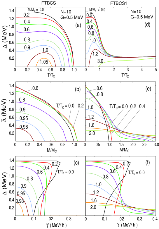
Figure 1: (Color online) Level-weighted pairing gaps $\bar{\Delta}$ as functions of $T$ at various $M$ [(a), (d)], and as functions of $M$ [(b), (e)] and $\gamma$ [(c), (f)] at several $T$ for $N$ = 10, $G$ = 0.5 MeV obtained within the FTBCS (left) and FTBCS1 (right).

Shown in Figs. 1 (a) and 1 (d) are the level-weighted pairing gaps $\bar{\Delta}$ as functions of $T$ at various $M$, whereas the dependence of $\bar{\Delta}$ on $M$ at several $T$ is displayed in Figs. 1 (b) and 1(e). Finally, Figs. 1 (c) and 1 (f) show the gaps $\bar{\Delta}$ as functions of the angular velocity $\gamma$ at various $T$. All the results are obtained for the system with $N$ = 10 and $G$ = 0.5 MeV, from which the left panels are the predictions by the FTBCS theory, whereas the right panels are those by the FTBCS1 one. It is clearly seen from Figs. 1 (a) and 1 (b) that the FTBCS gap decreases with increasing $T$ ($M$) at $M=$ 0 ($T=$ 0) up to a certain critical value $T_{\rm c}=$ 0.77 MeV ($M_{\rm c}=$ 8$\hbar$), where the FTBCS gap collapses. The collapse of the pairing gap at $M=M_{\rm c}$ (at $T=$ 0) was proposed by Mottelson and Valatin as being caused by the Coriolis force, which breaks the Cooper pairs MV . This feature remains with the FTBCS gap as a function of $M$, when $T\neq$ 0, but with decreasing $M_{\rm c}(T)<M_{\rm c}$ as $T$ increases beyond 0.6$T_{\rm c}$. As for the behavior of the FTBCS gap as a function of $T$, one notices that, at $M$ slightly larger than $M_{\rm c}$, the so-called thermally assisted pairing correlation takes place, in which the pairing gap is zero at $T\leq T_{1}$, increases at $T>T_{1}$ to reach a maximum, then decreases again to vanish at $T\geq T_{2}$ [See. Fig. 1 (a) for $M/M_{\rm c}\geq$ 1]. This interesting phenomenon was predicted and explained, for the first time, by Moretto in Refs. MorettoPLB35 ; MorettoNPA185 by applying the FTBCS to the uniform model. At $M/M_{\rm c}>$ 1.1, no FTBCS pairing gap remains.

Different from the FTBCS predictions, the results obtained within the FTBCS1 include the effect caused by the QNF. As one can see in Fig. 1 (d), while, in the region of low temperature $T<T_{\rm c}$, the FTBCS1 and FTBCS gaps for different $M$ are rather similar, they are qualitatively different at $T>T_{\rm c}$. Here, the QNF, which is rather strong at high $T$, causes a monotonous decrease of the FTBCS1 gap $\bar{\Delta}$ as $T$ increases. This FTBCS1 gap never collapses even at very high $T$. Instead all the values of the FTBCS1 gap obtained at various $M$ seem to saturate at a value of around 2.25 MeV at $T>$ 5 MeV. This feature shows that, the effect of angular momentum on reducing the pairing correlation is significant only at low $T$. In the high temperature region, the QNF leads to a persistence of the pairing correlation in a rotating system. Compared to the FTBCS theory, when the QNF is neglected, the effect of thermally assisted pairing correlation also takes place at $M/M_{\rm c}>1.1$. However, the FTBCS1 gap is now zero at $T\leq T_{1}$, reappears at $T=T_{1}$, and remains finite at $T>T_{1}$. This result is found in qualitative agreement with those obtained in the calculations of the canonical gap of in Ref. FrauendorfPRB68 , where the reappearance of the pairing gap at finite $T$ and $\gamma$ is related to the strong fluctuations of order parameter in the canonical ensemble of small systems such as metal clusters and nuclei. In the present paper, we point out the QNF as the microscopic origin of this effect. Comparisons between the FTBCS1 gaps and the canonical ones obtained at ($T\neq$ 0, $M=$ 0) and ($T=$ 0, $M$ and/or $\gamma\neq$ 0) are discussed later, in Sec. III.5.

The QNF has a similar effect on the behavior of the pairing gap $\bar{\Delta}$ as a function of angular momentum. As low $T$, when the QNF is still negligible, the FTBCS and FTBCS1 gaps as functions of $M$ are similar. They both decreases as $M$ increases, and collapse at $M=M_{\rm c}$ and at $M$ slightly higher than $M_{\rm c}$ for 0 $<T/T_{\rm c}\leq$ 0.2, contrary to the trend within the FTBCS theory, where $M_{\rm c}(T)$ decreases as $T/T_{\rm c}$ increases above 0.6 discussed above [Compare Figs. 1 (b) and 1 (e)]. At $T/T_{\rm c}=$ 0.8, e.g., the collapsing points of the FTBCS and FTBCS1 gaps are $M/M_{\rm c}\simeq$ 0.85, and 2.9, respectively.

The FTBCS and FTBCS1 pairing gaps are displayed in Figs. 1 (c) and 1 (f) as functions of angular velocity $\gamma$ at various $T$. For $T/T_{\rm c}\leq$ 0.2, the pairing gap undergoes a backbending, which will be discussed in the Sec. III.4. At $T/T_{\rm c}>$ 0.2 no backbending is seen for the pairing gaps. This result agrees with those obtained in calculations within the finite-temperature Hartree-Fock-Bogoliubov cranking (FTHFBC) theory, which is applied to the two-level model in Ref. GoodmanNPA352 . Within the FTBCS1, the pairing gaps at large $M$ become enhanced with $T$, in agreement with the results obtained within an exactly solvable model for a single $f_{7/2}$ shell in Ref. SheikhPRC72 .

III.3 Results for realistic nuclei

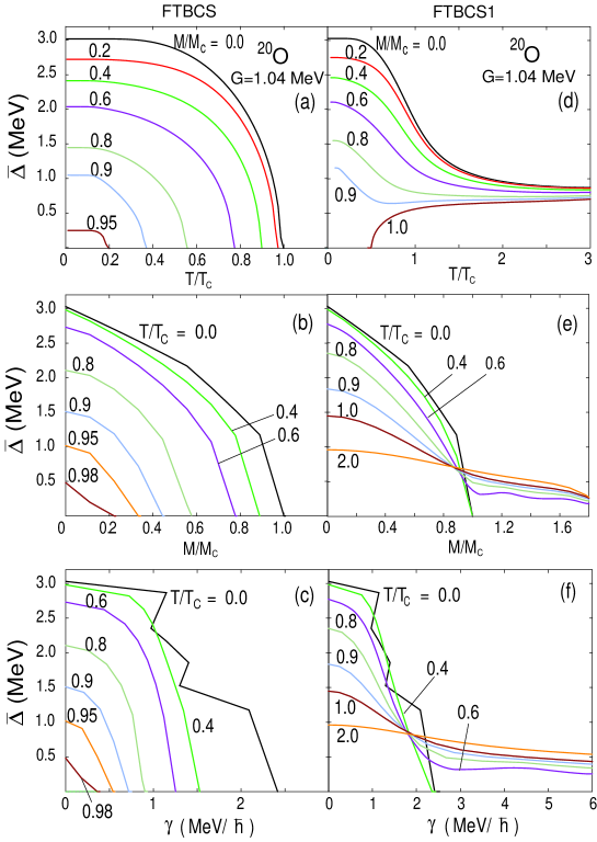
Figure 2: (Color online) Same as Fig. 1 but for neutrons in ²⁰O using $G=$ 1.04 MeV.

Shown in Fig. 2 are the level-weighted pairing gaps as functions of $T,M$ and $\gamma$ obtained within the FTBCS and FTBCS1 theories for neutrons in ²⁰O. The values of $T_{\rm c}$ (at $M=$ 0) and $M_{\rm c}$ (at $T=$ 0) are found equal to 1.57 MeV and 4$\hbar$, respectively. Compared to the case with schematic model discussed in the previous section, the difference is that no thermally assisted pairing correlation appears within the FTBCS for ²⁰O. All the FTBCS gaps behave similarly as functions of $T$ with increasing $M$. At a given value of $M$, they decrease with increasing both $T$, and collapse at some values $T_{\rm c}(M)<T_{\rm c}$. A similar behavior is seen for the gaps as functions of $M$ at a given value of $T$. Here the critical value $M_{\rm c}(T)$ for the angular momentum, at which the gap collapses is found decreasing with increasing $T$ so that $M_{\rm c}(T)<M_{\rm c}$ [See Figs. 2 (a) and 2 (b)]. Meanwhile, the temperature dependence of the FTBCS1 gap in Fig. 2 (d) shows a clear manifestation of the thermally assisted pairing gap. As $M$ increases up to $M/M_{\rm c}\simeq$ 0.8, the gap decreases monotonously with increasing $T$ up to $T\simeq$ 1.5$T_{\rm c}$, higher than which the gap seems to be rather stable against the variation of $T$. At $M/M_{\rm c}\geq$ 0.9, the reentrance of thermal pairing starts to show up as the enhancement of the tail at $T>T_{\rm c}$. When $M/M_{\rm c}$ becomes equal to or larger than 1, the gap completely vanishes at low $T$, but reappears starting from a certain value of $T$, above which the gap increases with $T$ and reach a saturation at high $T$. At $T\geq$ 3 MeV, all the gaps obtained at different values of $M$ seem to coalesce to limiting value around 0.7 – 0.8 MeV. At a given value of $T$ in the region $T/T_{\rm c}\leq$ 0.7, as shown in Fig. 2 (e), the pairing gaps decrease steeply with increasing $T$ and all collapse at the same value $M_{\rm c}$. This difference compared to the FTBCS theory comes from the presence of the QNF. At $T/T_{\rm c}\geq$ 0.8, the QNF becomes stronger, which pushes up the collapsing point to $M_{\rm c}(T)=2M_{\rm c}$. One can also sees some oscillation occurring in the region between 0.8 $\leq M/M_{\rm c}\leq$ 1.4 because of the shell structure. The collapsing point might be shifted even further to higher $M$ with increasing $T$, but at too high $T$ the temperature dependence of single-particle energies becomes significant so that the use of the spectrum obtained at $T=$ 0 is no longer valid BrackBonche .

The pairing gaps as functions of angular velocity $\gamma$ obtained at various $T$ within the FTBCS and FTBCS1 theories are plotted in Figs. 2 (c) and 2 (f), respectively. As $E_{k}$, $\gamma$ and $m_{k}$ are positive, at $T=0$, the quasiparticle occupation number $n_{k}^{-}$ is always zero, whereas $n_{k}^{+}$ is a step function of $E_{k}-\gamma m_{k}$, which is zero if $E_{k}>\gamma m_{k}$ and 1 if $E_{k}\leq\gamma m_{k}$. As the result, the FTBCS and FTBCS1 gaps decrease with increasing $\gamma$ in a stepwise manner up to a critical value $\gamma_{\rm c}$, where they vanish. At $T\neq$ 0, the Fermi-Dirac distribution replaces the step function, which washes out the stepwise manner in the behavior of the gaps as functions of the $\gamma$. Here again, once can see that, at $T/T_{\rm c}>$ 0.8, the QNF is so strong that the collapse of the FTBCS1 gap is completely smoothed out [Fig. 2 (f)].

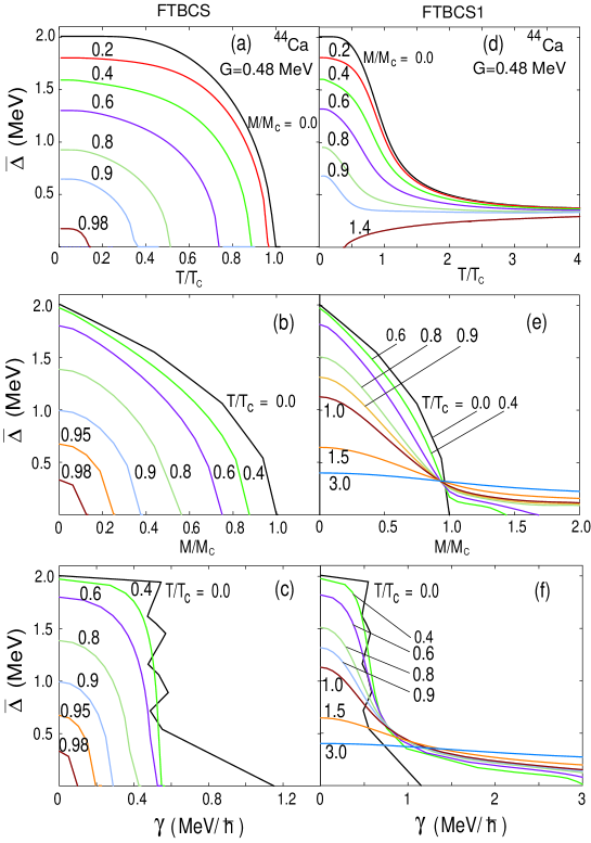
Figure 3: (Color online) Same as Fig. 1 but for neutrons in ⁴⁴Ca using $G=$ 0.48 MeV.

The level-weighted pairing gaps $\bar{\Delta}$ for neutrons in ⁴⁴Ca shown in Fig. 3 have a similar behavior as as functions of $T$, $M$ and $\gamma$ with the values of $T_{\rm c}$ and $M_{\rm c}$ are found to be 1.07 MeV and 8 $\hbar$, respectively. The thermally assisted pairing gap appears at $M/M_{\rm c}>$ 1.0 but the high-$T$ tail is much depleted due to a weaker QNF in a heavier system compared to that in ²⁰O.

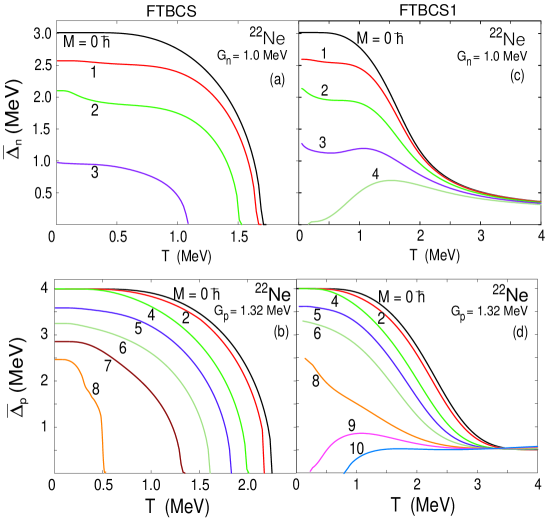
Figure 4: (Color online) Level-weighted pairing gaps as functions of $T$ at various $M$ obtained within the FTBCS (left) and FTBCS1 (right) for neutrons [(a), (c)], and protons [(b), (d)] in ²²Ne using $G_{n}=$ 1.0 MeV and $G_{p}=$ 1.32 MeV.

The well deformed nucleus ²²Ne has both neutron and proton open shells, therefore the gap and two number equations for protons ($p$) and neutrons ($n$) are simultaneously solved together with one equation for the total angular momentum $M=M_{p}+M_{n}$ to obtain the pairing gaps $\Delta_{p}$ and chemical potential $\lambda_{p}$ for protons, the corresponding quantities, $\Delta_{n}$ and $\lambda_{n}$, for neutrons, as well as the angular velocity $\gamma$ of the entire nucleus MorettoNPA216 . The level-weighted pairing gaps as functions of $T$ at several $M$ obtained for neutrons and protons in ²²Ne are shown in Fig. 4. The FTBCS neutron gaps become depleted with increasing $M$, and completely disappears at $M>3\hbar$. As a function of $T$, the FTBCS neutron gaps decrease as $T$ increases and collapse at $T_{\rm c}(M)$, which decreases from $T_{\rm c}(M=0)\simeq$ 1.7 MeV to $T_{\rm c}(M=3\hbar)\simeq$ 1.1 MeV. The FTBCS1 gaps obtained at $M<$ 3 $\hbar$ never collapse, but gradually decrease with increasing $T>T_{\rm c}(M=0)$, and remains a finite value of around 0.4 MeV at $T$ as high as 4 MeV. At $M=$ 4 $\hbar$, whereas there is no FTBCS gap, the thermally assisted pairing gap appears within the FTBCS1 theory at $T>$ 0, increases with $T$ to reach a maximum at $T\sim$ 1.5 MeV, then decreases slowly to reach the same high-$T$ limit of around 0.4 MeV at $T\simeq$ 4 MeV. The situation is the similar for the proton pairing gaps, where the effect of thermally assisted pairing correlation takes place at $M>$ 8 $\hbar$ with the rather stable values of the gap against $T>$ 3 MeV.

III.4 Backbending

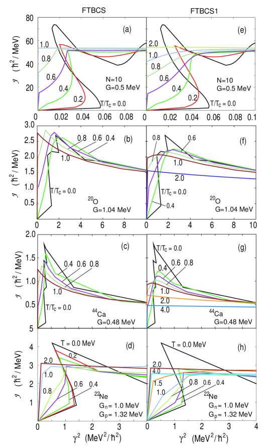
Figure 5: (Color online) Moment of inertia as a function of the square $\gamma^{2}$ of angular velocity $\gamma$ obtained within the FTBCS (left) and FTBCS1 (right) at various $T$ for $N=10$ [(a), e)], neutrons in ²⁰O [(b), (f)] and ⁴⁴Ca [(c), (g)], and the whole ²²Ne nucleus (including both proton and neutron gaps) [(d), (h)].

For an object that rotates about a fixed symmetry axis, its moment of inertia ${\cal J}$ is found as the total angular momentum $M$ divided by the angular velocity $\gamma$, i.e. ${\cal J}=M/\gamma$. The backbending phenomenon is most easily demonstrated by the behavior of ${\cal J}$ as a function of the square $\gamma^{2}$. This curve first increases with $\gamma^{2}$ up to a certain region of $\gamma^{2}$, where the increase suddenly becomes very steep, and the curve even bends backward. This phenomenon is understood as the consequence of the no-crossing rule in the region of band crossing LL . The SN phase transition has been suggested as one of microscopic interpretations of backbending MV .

The values of the moment of inertia ${\cal J}$, obtained at various $T$ within the schematic model as well as realistic nuclei, is plotted in Fig. 5. In the schematic model, one can see in Figs. 5 (a) and 5 (e) a sharp backbending, which takes place at very low temperatures, $T/T_{\rm c}\leq 0.2$. As the QNF is negligible in this temperature region, the predictions by the FTBCS and FTBCS1 theories are almost identical. As $T$ increases, the moment of inertia obtained within the FTBCS changes abruptly to reach the rigid-body value, generating a cusp, whereas, under the effect of QNF, the value obtained within the FTBCS1 theory gradually approaches the rigid-body value in such a way that the cusp is smoothed out. While no signature of backbending is seen in the results obtained in ²⁰O [Figs. 5 (c) and 5 (f)] and ⁴⁴Ca [Figs. 5 (d) and 5(g)], backbending can be seen in ²²Ne [Figs. 5 (d) and 5 (h)] at $T\leq$ 0.4 MeV in agreement with the experimental data reported in Ref. SzantoPRL42 .

III.5 Corrections due to SCQRPA and particle-number projection

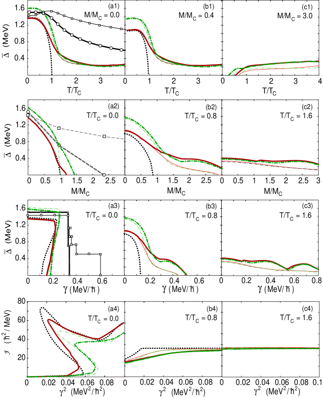
Figure 6: (Color online) Level-weighted pairing gap $\bar{\Delta}$ and moment of inertia ${\cal J}$ for $N=$ 10 with $G=$ 0.5 MeV [$\varepsilon=$ 0.1 MeV in Eqs. (43) and (44)]. (a1) – (c1): $\bar{\Delta}$ vs temperature $T$ at different angular momenta $M$. (a2) – (c4): Results obtained at different values of $T$, namely, (a2) – (c2): $\bar{\Delta}$ vs $M$; (a3) – (c3): $\bar{\Delta}$ vs angular velocity $\gamma$; (a4) – c4): ${\cal J}$ vs $\gamma^{2}$. The dotted, thin solid, thick solid, thin dash-dotted, thick dash-dotted lines are results obtained within the FTBCS, FTBCS1, FTBCS1+SCQRPA, FTLN1, FTLN1+SCQRPA, respectively. The solid lines with circles and boxes in (a1) and (a3) correspond to two definitions $\Delta_{\rm c}^{(1)}$ and $\Delta_{\rm c}^{(2)}$ of the canonical gaps at $T=0$, respectively (See Appendix A). In (a2) the dashed lines connecting the discrete values of the corresponding canonical gaps at $T=0$ are drawn to guide the eye.

Shown in Fig. 6 are the level-weighted pairing gaps and moment of inertia, obtained within the schematic model with $N=$ 10, where predictions offered by several approaches, namely the FTBCS, FTBCS1, FTBCS1 + SCQRPA, FTLN1, and FTLN1 + SCQRPA, are collected. In the same figure, the canonical gaps $\Delta_{\rm C}^{(1)}$ and $\Delta_{\rm C}^{(2)}$ obtained at ($T\neq$ 0, $M=$ 0) [Fig. 6 (a1)], ($T=0$, $M\neq$ 0) [Fig. 6 (a2)], and ($T=0$, $\gamma\neq$ 0) [Fig. 6 (a3)], are also shown (See Appendix A for the detailed discussion of the canonical results).

As seen from Figs. 6, the effect due to the SCQRPA corrections on the pairing gap increases with $M$. At $M/M_{\rm c}\leq$ 0.8 it is rather weak, causing only a slight enhancement of the gap at 1.2 $<T\leq$ 2 MeV as compared with the FTBCS1 results [Figs. 6 (a1) and 6 (b1)]. However, it becomes important at $M>1.2M_{\rm c}$ [Figs. 6 (c1), 6 (a2) – 6 (c2)], or $\gamma>$ 0.2 MeV$/\hbar$ (at $T\geq 0.8T_{\rm c}$) [Figs. 6 (b3) and 6 (c3)]. In particular, the reappearance of the thermal gap at $M\geq 1.1M_{\rm c}$ is significantly enhanced by the SCQRPA corrections [Figs. 6 (c1) and 6 (c2)]. For the moment of inertia [Figs. 6 (a4) – 6 (c4)], the SCQRPA corrections are important only at low $T$ and $\gamma<$ 0.25 MeV$/\hbar$. At $T>$ 1 MeV, the predictions by all the approximations for ${\cal J}$ saturate to the rigid-body value.

As compared to the predictions by the FTBCS1 and FTBCS1+SCQRPA, the corrections due to LN-PNP are important only at low $T$ and $M$. As the result, the gap is pushed up to be closer to the canonical results at $T\leq T_{\rm c}$ and $M=0$ [Fig. 6 (a1)]. This feature is well-known and has been discussed within the present approach at $M=$ 0 in Ref. DangHungPRC2008 . At $M\neq$ 0 ($\gamma\neq$ 0), the effect due to LN-PNP is noticeable in the gaps as functions of $M$ (or $\gamma$) only at [$M\leq$ 1.2$M_{\rm c}$ ($\gamma<$ 0.2 MeV$/\hbar$), $T<$ 1 MeV], otherwise the FTLN1 (FTLN1+SCQRPA) results are hardly distinguishable from the FTBCS1 (FTBCS1+SCQRPA) ones [Figs. 6 (b2), 6 (c2), 6 (b3), and 6 (c3)]. Consenquently, for the moment of inertia, the LN-PNP corrections to the FTBCS1 (FTBCS1+SCQRPA) results are important only at ($T<T_{\rm c}$, $\gamma<\gamma_{\rm c}$) [Figs. 6 (a4) – 6 (c4)]. In particular, the results at $T=$ 0 [Fig. 6 (a4)], where the BCS1 coincides with the BCS, show that, backbending becomes less pronounced within the SCQRPA and LN-SCQRPA. For this reason, the corrections due to LN-PNP are omitted in the results obtained for realistic nuclei below.

Shown in Figs. 7 and 8 are the pairing gaps, total energies and heat capacities as functions of $T$ obtained at $M/M_{\rm c}=$ 0, 0.4, and 0.8 within the FTBCS, FTBCS1 and FTBCS1 + SCQRPA for realistic nuclei, ²⁰O and ⁴⁴Ca. The SCQRPA corrections are significant for the total energy in the light nucleus, ²⁰O, due to the important contributions of the screening factors (27) and (28) HungDangPRC76 ; DangHungPRC2008 . In medium ⁴⁴Ca nucleus, the effect of SCQRPA corrections on the total energy is weaker. The corrections due to LN particle-number projection have a similar effect as that discussed above for the schematic model, but with much reduced magnitudes, so they are not shown in these figures. With increasing $M$ the pairing gap decreases. As the result, the total energy becomes larger but the relative effect of the SCQRPA correction does not change. For the heat capacity, as has been reported in Ref.  DangHungPRC2008 , the spike at $T_{\rm c}$ obtained within the FTBCS theory, which serves as the signature of the sharp SN phase transition, is smeared out within the FTBCS1 theory into a bump in the temperature region around $T_{\rm c}$. With increasing $M$, this bump becomes depleted further. Finally, the SQRPA corrections erase all the traces of the sharp SN phase transition in the model case as well as realistic nuclei.

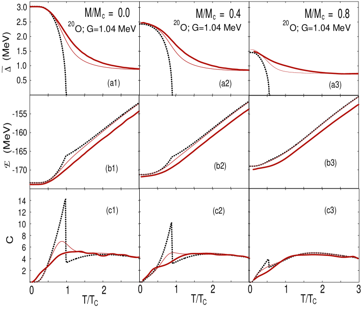
Figure 7: (Color online) Level-weighted pairing gaps $\bar{\Delta}$, total energies ${\cal E}$, and heat capacities $C$ as functions of temperature $T$ for three values of angular momentum $M$ obtained within the FTBCS (dotted lines), FTBCS1 (thin solid lines) and FTBCS1 + SCQRPA (thick solid lines) for neutrons in ²⁰O with $G=$ 1.04 MeV ($\varepsilon=$ 0.1 MeV).

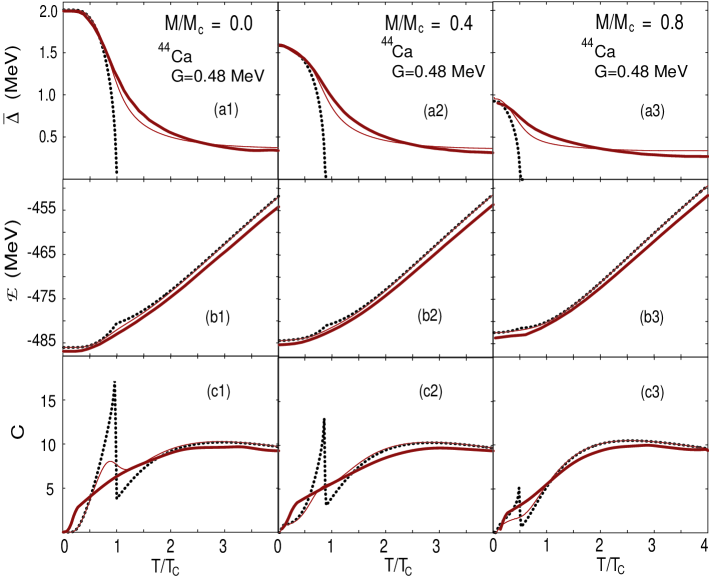
Figure 8: (Color online) Same as in Fig. 7 but for neutrons in ⁴⁴Ca with $G=$ 0.48 MeV ($\varepsilon=$ 0.1 MeV).

IV CONCLUSIONS

The present work extends the FTBCS1 (FTBCS1 + SCQRPA) theory to finite angular momentum to study the pairing properties of hot nuclei, which rotate noncollectively about the symmetry axis. The FTBCS1 theory includes the quasiparticle number fluctuation whereas the FTBCS1 + SCQRPA also takes into account the correction due to dynamic coupling to SCQRPA vibrations. The proposed extension is tested within the doubly degenerate equidistant model with $N=10$ particles as well as some realistic (spherical and deformed) nuclei, ²⁰O, ²²Ne, and ⁴⁴Ca. The numerical calculations were carried out within the FTBCS, FTBCS1, and FTBCS1 + SCQRPA for the pairing gap, total energy, and heat capacity as functions of temperature $T$, total angular momentum $M$, and angular velocity $\gamma$. The corrections due to the Lipkin-Nogami particle-number projection are also discussed. The analysis of the numerical results- allows us to draw the following conclusions:

1. The proposed approach is able to reproduce the effect of thermally assisted pairing correlation that takes place in the schematic model within the FTBCS theory, according to which a finite pairing gap can reappear within a given temperature interval, $T_{1}<T<T_{2}$ ($T_{1}>0$), while it is zero beyond this interval. However, this phenomenon does not show up in realistic nuclei under consideration.

2. Under the effect of QNF, the paring gaps obtained within the FTBCS1 at different values $M$ of angular momentum decrease monotonously as $T$ increases, and do not collapse even at hight $T$ in the schematic model as well as realistic nuclei. The effect of thermally assisted pairing correlation is seen in all the cases, but in such a way that the pairing gap reappears at a given $T_{1}>$ 0 and remains finite at $T>T_{1}$, in qualitative agreement with the canonical results of Ref. FrauendorfPRB68 .

3. The backbending of the moment of inertia is found in the schematic model and in ²²Ne in the low temperature region, whereas it is washed out with increasing temperature. This effect does not occur in ²⁰O and ⁴⁴Ca, in consistent with existing experimental data and results of other theoretical approaches.

4. The effect caused by the corrections due to the dynamic coupling to SCQRPA vibrations on the pairing gaps, total energies, and heat capacities is found to be significant in the region around the critical temperature $T_{\rm c}$ of the SN phase transition and/or at large angular momentum $M$ (or angular velocity $\gamma$). It is larger in lighter systems. As the result, all the signatures of the sharp SN phase transition are smoothed out in both schematic model and realistic nuclei. The SCQRPA corrections also significantly enhance the reappearance of the thermal gap at finite angular momentum. On the other hand, the effect caused by the corrections due to PNP is important only at temperatures below $T_{\rm c}$, and at quite low angular momentum. In particular, it makes backbending less pronoucned at $T=$ 0.

Still the fluctuations due to violation of angular-momentum conservation are not implemented in the present extension. We hope that further studies in this direction will shed light on this issue.

Appendix A On the comparison with canonical results

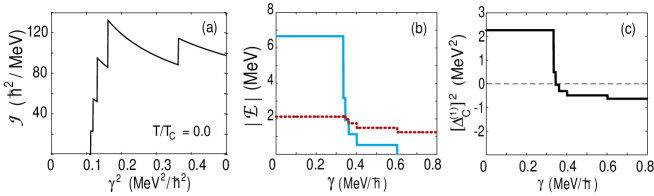
Figure 9: (Color online) (a) Canonical moment of inertia vs $\gamma^{2}$; (b): Absolute values $|\langle{\cal E}\rangle_{\rm C}-{\cal E}_{\rm m.f.}|$ (solid line) and $|{\cal E}_{\rm unc.}|$ (dotted line) vs $\gamma$; (c): $[\Delta_{\rm C}^{(1)}]^{2}$ vs $\gamma$ for the schematic model with $N=$ 10 and $G=$ 0.5 MeV at $T=$ 0.

It has been shown in Sec. III.2 that the FTBCS1 (FTBCS1+SCQRPA) produces results in qualitative agreement with the canonical ones of Ref. FrauendorfPRB68 , in particular, the reappearance of the thermal gap at $M\neq$ 0. However, it is important to make clear the difference between the predictions by BCS-based approaches and the canonical results. As a matter of fact, the $z$-projection $M$ of the total angular momentum within the FTBCS (FTBCS1) approach is temperature-independent. At $T$ varies, by solving the FTBCS (FTBCS1) equations, the angular velocity $\gamma$ is defined as a Lagrangian multiplier so that $M$, being the thermal average of the total angular momentum within the grand canonical ensemble (12), remains unchanged. In this way, within the FTBCS (FTBCS1), the angular velocity $\gamma$ varies with $T$, whereas $M$ does not. Similar to that for choosing the chemical potential $\lambda$ to preserve the (grand-canonical ensemble) average particle-number $N$, this contraint is physically reasonable when the total angular momentum is conserved as in the noncollective rotation of spherical systems or rotation of axially symmetric systems about the symmetry axis, as has been discussed in Sec. II.1.

On the contrary, the canonical results in Ref. FrauendorfPRB68 are obtained by embedding the eigenvalues $E_{\nu,i}(\gamma)=E_{\nu}-\gamma M_{\nu,i}$ in the canonical ensemble with the partition function

$$Z(\beta,\gamma)=\sum_{\nu,i}e^{-\beta E_{\nu,i}(\gamma)}~{}.$$ (49)

Here $E_{\nu}$ denote the eigenvalues of the $\nu$th state with seniority $\nu$ at $\gamma=$ 0, whereas $M_{\nu,i}$ are the z-projections of angular momenta of $\nu$ nucleons. While the eigenvalues $E_{\nu}$ are obtained by separately diagonalizing the pairing Hamiltonian $H_{P}$ in Eq. (2), the rotational part $\Phi_{\nu}=\sum_{i}\exp(\beta\gamma M_{\nu,i})$ of the partition function $Z(\beta,\gamma)$ is calculated following Ref. Kuzmenko . The resulting canonical average value $\langle M(\beta,\gamma)\rangle_{\rm C}=\beta Z(\beta,\gamma)^{-1}\partial{Z(\beta,\gamma)}/\partial{\gamma}$ of angular momentum, therefore, varies with $T$. On the other hand, the angular velocity $\gamma$ just plays the role of an independent parameter, therefore, does not depend on $T$. By the same reason, each canonical average value $\langle M(\beta,\gamma)\rangle_{\rm C}$ corresponds to a single value of $\gamma$, i.e. the canonical moment of inertia ${\cal J}_{\rm C}$ undergoes no backbending, as shown in Fig. 9 (a).

Because of this principal difference, a quantitative comparison between the FTBCS (FTBCS1) results, and the canonical ones as functions of $M$ (or $\gamma$) at $T\neq$ 0 unfortunately turns out to be impossible. To establish a meaningful correspondence, one needs to know the exact eigenvalues of the ground state as well as all excited states of the pairing problem described by Hamiltonian (1) so that, by embedding the eigenvalues in the grand canonical ensemble, $\gamma$ becomes a function of $T$ in such a way to keep $\langle M(\beta,\gamma)\rangle_{\rm C}$ always equal to $M$. To our knowledge, this problem still remains unsolved. One may also try to estimate the results within the microcanonical ensemble. However, here one faces a problem of extracting the nuclear temperature, which is rather ambiguous at low level density (small $N$) within the schematic model under consideration Sumaryada ; DangHung , whereas the extension of exact solution of the pairing problem to $T\neq$ 0 is unpracticable at $N\geq$ 16.

Therefore, in the present paper, we can only compare the predictions of our approach with the canonical results as functions of temperature $T$ at $M=$ 0, or as functions of $M$ (or angular velocity $\gamma$) at $T=$ 0. For this purpose, and given several definitions of the “effective” gaps existing in literature, we choose to employ in the present paper two definitions of the canonical gaps, $\Delta_{\rm C}^{(1)}$ and $\Delta_{\rm C}^{(2)}$. They should be understood as effective ones since a gap per se, which is a mean-field concept, does not exist in the exact solutions of the pairing problem.

The canonical gap $\Delta_{\rm C}^{(1)}$ is defined from the pairing energy ${\cal E}_{\rm pair}$ of the system as

$$[\Delta_{C}^{(1)}]^{2}={-G{\cal E}_{\rm pair}}~{},\hskip 8.53581pt{\cal E}_{\rm pair}\equiv\langle{\cal E}\rangle_{\rm C}-{\cal E}_{\rm m.f.}-{\cal E}_{\rm unc.}~{},\hskip 8.53581pt{\cal E}_{\rm m.f.}\equiv 2\sum_{k}\epsilon_{k}f_{k}~{},\hskip 8.53581pt{\cal E}_{\rm unc.}\equiv-{G}\sum_{k}f_{k}^{2}~{}.$$ (50)

Here $\langle{\cal E}\rangle_{\rm C}$ is the total energy within the canonical ensemble with the partition function $Z(\beta,\gamma)$ given by Eq. (49) of a system rotating at angular velocity $\gamma$, or with the partition function $Z(\beta,0)$ at $M=$ 0. The term ${\cal E}_{\rm m.f.}$ denotes the energy of the single-particle motion described by the first term at the right-hand side of the pairing Hamiltonian $H_{P}$ in Eq. (2). Functions $f_{k}$ are occupation numbers of $k$th orbitals within the canonical ensemble. The energy ${\cal E}_{\rm m.f.}$ becomes that of the mean-field once the single-particle occupation numbers $f_{k}$ are replaced with those describing the Fermi-Dirac distributions of independent particles. The energy ${\cal E}_{\rm unc.}$ comes from the uncorrelated single-particle configurations caused by the pairing interaction in Hamiltonian (2). Therefore, by subtracting the term ${\cal E}_{\rm m.f.}+{\cal E}_{\rm unc.}$ from the total energy $\langle{\cal E}\rangle_{\rm C}$, one obtains the result that corresponds to the energy due to pure pairing correlations. The definition (50) is very similar to that given in Ref. Delft . It is, however, different from the canonical gap $\Delta_{\rm C}^{(2)}$, which is used in Refs. FrauendorfPRB68 . The latter is defined as

$$[\Delta_{\rm C}^{(2)}]^{2}={-G\big{[}\langle{\cal E}\rangle_{\rm C}-\langle{\cal E}(G=0)\rangle_{\rm C}\big{]}}~{},$$ (51)

where $\langle{\cal E}(G=0)\rangle_{C}$ is the total canonical energy $\langle{\cal E}\rangle_{\rm C}$ at $G=$ 0.

The canonical gaps $\Delta_{\rm C}^{(1)}$ and $\Delta_{\rm C}^{(2)}$ are shown in Figs. 6 (a1), 6 (a2), and 6 (a3) as functions of temperature $T$ (at $M=$ 0), angular momentum $M$ (at $T=$ 0), and angular velocity $\gamma$ (at $T=$ 0), respectively. It is seen from these figures that the difference between the two canonical gaps $\Delta_{\rm C}^{(1)}$ and $\Delta_{\rm C}^{(2)}$ is rather significant at large $T$ for $M=$ 0, and at large $M$ (or $\gamma$) for $T=$ 0. The reason is rather simple since the definition (50) of $\Delta_{\rm C}^{(1)}$ is rather similar to that for the BCS gap. As a matter of fact, by replacing the canonical single-particle occupation numbers $f_{k}$ with the Bogoliubov’s coefficients $v_{k}^{2}$, and the total energy $\langle{\cal E}\rangle_{\rm C}$ with that obtained within the BCS theory, the gap $\Delta_{\rm C}^{(1)}$ reduces to the usual BCS gap. Meanwhile, by doing so with $\Delta_{\rm C}^{(2)}$, the energy $\langle{\cal E}(G=0)\rangle_{\rm C}$ just reduces to the Hartree-Fock energy, leaving the uncorrelated energy ${\cal E}_{\rm unc.}$ out of the definition. Consequently, as functions of $T$, the gaps predicted by the BCS-based approaches under consideration agree better with the canonical gap $\Delta_{\rm C}^{(1)}$ than with $\Delta_{\rm C}^{(2)}$ [Fig. 6 (a1)].

As functions of angular velocity $\gamma$, both the squared values (50) and (51) of the canonical gaps undergo a stepwise decrease with increasing $\gamma$. The step occurs whenever the state of the lowest energy changes from $\nu-2$ to $\nu$, causing a stepwise increase of $\langle M(\beta,\gamma)\rangle_{\rm C}$ FrauendorfPRB68 . Therefore, for $N=$ 10, the pairs are gradually broken in 5 steps with a corresponding stepwise increase of seniority $\nu$ from 0 to 10 by two units in each step. However, Fig. 9 (b) shows that the absolute value of the uncorrelated energy ${\cal E}_{\rm unc.}$, which enters in the definition (50) of the gap $\Delta_{\rm C}^{(1)}$, becomes larger than that of the difference ${\cal E}_{\rm C}-{\cal E}_{\rm m.f.}$ already at the second step, leading to $[\Delta_{\rm C}^{(1)}]^{2}<$ 0 [Fig. 9 (c)], i.e. an imaginary value for $\Delta_{\rm C}^{(1)}$. As the result, instead of collapsing as $\Delta_{\rm C}^{(2)}$ in 5 steps at a rather large value of $M$ (or $\gamma$), the canonical gap $\Delta_{\rm C}^{(1)}$ collapses in two steps at a value of $M$ (or $\gamma$) much closer to $M_{\rm c}$ (or $\gamma_{\rm c}$) for the BCS gap [Figs. 6 (a2) and 6 (a3)]. Once again, this makes the gaps predicted by the BCS-based approaches as functions of $M$ (or $\gamma$) agree better with the canonical gap $\Delta_{\rm C}^{(1)}$, rather than with $\Delta_{\rm C}^{(2)}$ [Figs. 6 (a2) and 6 (a3)].

References

- (1) J. Bardeen, L. Cooper, and Schrieffer, Phys. Rev. C 108, 1175 (1957).
- (2) H. Ding et al., Nature 382, 51 (1996).
- (3) L. G. Moretto, Phys. Lett. B 40, 1 (1972).
- (4) A. L. Goodman, Phys. Rev. C 29, 1887 (1984).
- (5) R. Rossignoli, P. Ring and N. D. Dang, Phys. Lett. B 297, 9 (1992).
- (6) N. D. Dang, P. Ring and R. Rossignoli, Phys. Rev. C 47, 606 (1993).
- (7) N. Dinh Dang and V. Zelevinsky, Phys. Rev. C 64, 064319 (2001).
- (8) N. Dinh Dang and A. Arima, Phys. Rev. C 67, 014304 (2003).
- (9) N. D. Dang, Nucl. Phys. A 784, 147 (2007).
- (10) A. Schiller et al., Phys. Rev. C 63, 021306(R) (2001).
- (11) N. Dinh Dang and N. Quang Hung, Phys. Rev. C 77, 064315 (2008).
- (12) N. Q. Hung and N. D. Dang, Phys. Rev. C76, 054302 (2007); Ibid. 77, 029905 (E) (2008).
- (13) R.W. Richardson, Phys. Lett. 3, 277 (1963); 5, 82 (1963); R.W. Richardson and N. Sherman, Nucl. Phys. 52, 221 (1964).
- (14) A. Volya, B.A. Brown, and V. Zelevinsky, Phys. Lett. B 509 (2001) 37.
- (15) S. Rombouts, K. Heyde, and N. Jachowicz, Phys. Rev. C 58, 3295 (1998).
- (16) T. Kammuri, Prog. Theor. Phys. 31, 595 (1964).
- (17) L. G. Moretto, Phys. Lett. B 35, 397 (1971).
- (18) L. G. Moretto, Nucl. Phys. A 185, 145 (1971).
- (19) R. Balian, H. Flocard and M. Vénéroni, Phys. Rep. 317, 251 (1999).
- (20) S. Frauendorf, N. K. Kuzmenko, V. M. Mikhajlov, and J. A. Sheikh, Phys. Rev. B 68, 024518 (2003).
- (21) J. A. Sheikh, R. Palit, and S. Frauendorf, Phys. Rev. C 72, 041301(R) (2005).
- (22) A. Bohr and B.R. Mottelson, Physica Scripta, 10 A, 13 (1974).
- (23) J. Högaasen-Feldman, Nucl. Phys. 28, 258 (1961).
- (24) N. D. Dang, Z. Phys. A 335, 253 (1990).
- (25) N.N. Bogolyubov and S.V. Tyablikov, Soviet Phys.-Doklady 4, 60 (1959) [Dokl. Akad. Nauk SSSR 126, 53 (1959)].
- (26) D.N. Zubarev, Soviet Physics Uspekhi 3, 320 (1960) [Usp. Fiz. Nauk 71, 71 (1960)].
- (27) H.J. Lipkin, Ann. Phys. 9, 272 (1960); Y. Nogami, Phys. Rev. 134, B313 (1964); H.C. Pradhan, Y. Nogami, and J. Law, Nucl. Phys. A 201, 357 (1973).
- (28) E. M. Szanto, et. al., Phys. Rev. Lett. 42, 622 (1979).
- (29) S. Cwiok, J. Dudek, W. Nazarewicz, J. Skalski, and T. Werner, Computer Physics Communications 46, 379 (1987).
- (30) R. Id Betan, N. Sandulescu, and T. Vertse, Nucl. Phys. A 771, 93 (2006).
- (31) B.R. Mottelson and J.G. Valatin, Phys. Rev. Lett. 5, 511 (1960).
- (32) N.K. Kuzmenko and V.M. Mikhajlov, arXiv:cond-mat/0002030v1; Phys. Lett. A 296, 49 (2002).
- (33) A. L. Goodman, Nucl. Phys. A 352, 45 (1981).
- (34) M. Brack and P. Quentin, Phys. Lett. B 42, 159 (1974); P. Bonche, S. Levit, and D. Vautherin, Nucl. Phys. A 427, 178 (1984).
- (35) L.G. Moretto, Nucl. Phys. A 216, 1 (1973).
- (36) L.D. Landau and E.M. Lifshitz, Course of Theoretical Physics (Pergamon, Oxford, 1959).
- (37) J. von Delft and D.C. Ralph, Phys. Rep. 345, 61 (2001).
- (38) T. Sumaryada and A. Volya, Phys. Rev. C 76, 024319 (2007).
- (39) N.Q. Hung and N. Dinh Dang, submitted.